Inconsistency in the ordinal pairwise comparisons method
with and without ties

Konrad Kułakowski konrad.kulakowski@agh.edu.pl AGH University of Science and Technology, Krakï¿œw, Poland

Abstract

Comparing alternatives in pairs is a well-known method of ranking creation. Experts are asked to perform a series of binary comparisons and then, using mathematical methods, the final ranking is prepared. As experts conduct the individual assessments, they may not always be consistent. The level of inconsistency among individual assessments is widely accepted as a measure of the ranking quality. The higher the ranking quality, the greater its credibility.

One way to determine the level of inconsistency among the paired comparisons is to calculate the value of the inconsistency index. One of the earliest and most widespread inconsistency indices is the consistency coefficient defined by Kendall and Babington Smith. In their work, the authors consider binary pairwise comparisons, i.e., those where the result of an individual comparison can only be: better or worse. The presented work extends the Kendall and Babington Smith index to sets of paired comparisons with ties. Hence, this extension allows the decision makers to determine the inconsistency for sets of paired comparisons, where the result may also be "equal." The article contains a definition and analysis of the most inconsistent set of pairwise comparisons with and without ties. It is also shown that the most inconsistent set of pairwise comparisons with ties represents a special case of the more general set cover problem.

keywords:

pairwise comparisons, consistency coefficient , inconsistency , AHP

1 Introduction

The use of pairwise comparisons (PC) to form judgments has a long history. Probably the first who formally defined and used pairwise comparisons for decision making was Ramon Llull (the XIII century) [6]. He proposed a voting system based on binary comparisons. The subject of comparisons (alternatives) were people - candidates for office. Voters evaluated the candidates in pairs, deciding which one was better. In the XVIII century, Llull’s method was rediscovered by Condorcet [7], then once again reinvented in the middle of the XX century by Copeland [6, 8]. At the beginning of the XX century, Thurstone used the pairwise comparisons method (PC method) quantitatively [39]. In this approach, the result returned does not only contain information about who or what is better, but also indicates how strong the preferences are. Later, both approaches, ordinal (qualitative), as proposed by Llull, and cardinal (quantitative), as used by Thurstone, were developed in parallel. Comparing alternatives in pairs plays an important role in research into decision making systems [14, 17, 29], ranking theory [34, 21], social choice theory [38], voting systems [40, 12, 41] and others.

In general, the PC method is a ranking technique that allows the assessment of the importance (relevance, usefulness, competence level etc.) of a number of alternatives. As it is much easier for people to assess two alternatives at a time than handling all of them at once, the PC method assumes that, first, all the alternatives are compared in pairs, then, by using an appropriate algorithm, the overall ranking is synthesized. The choice of the algorithm is not easy and is still the subject of research and vigorous debate [35, 42, 28]. Of course, it also depends on the nature of the comparisons. The cardinal methods use different algorithms [19, 13] than the ordinal ones [21, 6, 20, 40]. Despite the many differences between ordinal and cardinal pairwise comparisons, both approaches have much in common. For example, both approaches use the idea of inconsistency among individual comparisons. The notion of inconsistency introduced by the pairwise comparisons method is based on the natural expectation that every two comparisons of any three different alternatives should determine the third possible comparison among those alternatives.

To better understand the phenomenon of inconsistency, let us assume that we have to compare three alternatives $c_{1},c_{2}$ and $c_{3}$ with respect to the same criterion. If after the comparison of $c_{1}$ and $c_{2}$ it is clear to us that $c_{2}$ is more important than $c_{2}$ , and similarly, after comparing $c_{2}$ and $c_{3}$ it is evident that $c_{3}$ is more important than $c_{1}$ then we may expect that $c_{3}$ will also turn out to be more important than $c_{1}.$ The situation in which $c_{1}$ is better than $c_{3}$ would raise our surprise and concern. That is because it seems natural to assume that the preferential relationship should be transitive. If it is not, we have to deal with inconsistency. As pairwise comparisons are performed by experts, who, like all human beings, sometimes make mistakes, the phenomenon of inconsistency is something natural. The ranking synthesis algorithm must take it into account. On the other hand, if a large number of such “mistakes” can be found in the set of paired comparisons, one can have reasonable doubts as to the credibility of the ranking obtained from such lower quality data.

Both ordinal and cardinal PC methods developed their own solutions for determining the degree of inconsistency. Research into the cardinal PC method resulted in a number of works on inconsistency indices. Probably the most popular inconsistency index was defined by Saaty in his seminal work on the Analytic Hierarchy Process (AHP) [34]. His work prompted others to continue the research [27, 32, 1, 37, 3, 5]. The ordinal PC methods also have their own ways of assessing the level of inconsistency. In their seminal work [26] Kendall and Babington Smith introduced the inconsistency index (called by the authors the consistency coefficient). Their index allows the inconsistency degree of a set composed of binary pairwise comparisons to be determined. The results obtained by the authors were the inspiration for many other researchers in different fields of science [23, 30, 31, 2, 4, 36].

Although the ordinal pairwise comparisons method is a really powerful and handy tool facilitating the right decision, in practice we very often face the problem that the two options seem to be equally important. In such a situation, we can try to get around the problem by a brute force method of breaking ties. For example, we can do this by “instructing the judge to toss a mental coin when he cannot otherwise reach a decision; or, allowing him the comfort of reserving judgment, we can let a physical coin decide for him” [9, p. 94 - 95]. It is clear, however, that instead of relying on more or less arbitrary methods of breaking ties, it is better to accept their existence and incorporate them into the model. Indeed, ties have been inextricably linked with the ranking theory for a long time [6, 25, 9]. The ordinal pairwise comparisons method with ties has its own techniques of synthesizing ranking [15, 10, 40]. In this perspective, research into the inconsistency of ordinal pairwise comparisons with ties is quite poor. In particular, the consistency coefficient as defined by [26] is not suitable for determining the inconsistency of PC with ties. The problem was recognized by Jensen and Hicks [22], and later by Iida [18]. These authors also made attempts to patch up this gap in the ranking theory, however, the fundamental question as to what extent the set of PC with ties can be inconsistent still remains unanswered.

The purpose of the present article is to answer this question, and thus to define the inconsistency index for the ordinal PC with ties in the same manner as Kendall and Babington Smith did [26] for binary PC. The definition of the inconsistency index is accompanied by a thorough study of the most inconsistent sets of pairwise comparisons with and without ties.

The article is composed of eight sections including the introduction and four appendices. The PC with ties is formally introduced in the next section (Sec. 2). For the purpose of modeling PC with ties, a generalized tournament graph has also been defined there. The most inconsistent set of binary PC is studied in (Sec. 3). It is also proven that the number of inconsistent triads in such a graph is determined by Kendall Babington Smith’s consistency coefficient. The next section (Sec. 4) describes how the most inconsistent set of PC with ties may look. Thus, it contains several theorems describing the quantitative relationship between the elements of the generalized tournament graph. Finally, in (Sec. 5) the most inconsistent set of PC with ties is proposed. The generalized inconsistency index for ordinal PC is also defined (Sec. 6). The penultimate section (Sec. 7) contains a discussion of the subject. In particular, the relationship between the maximally inconsistent set of PC and the NP-complete set cover problem [24] is shown. A brief summary is provided in (Sec. 8).

2 Model of inconsistency

Let us suppose we have a number of possible choices (alternatives, concepts) $c_{1},\ldots,c_{n}$ where we are able to decide only whether one is better (more preferred) than the other or whether both alternatives are equally preferred. In the first case, we will write that $c_{i}\prec c_{j}$ to denote that $c_{j}$ is more preferred than $c_{i}$ , whilst in the second case, to express that two alternatives $c_{i}$ and $c_{j}$ are equally preferred we write $c_{i}\sim c_{j}$ . The preference relationship is total. Hence, for every two $c_{i}$ and $c_{j}$ it holds that either $c_{i}\prec c_{j}$ , $c_{j}\prec c_{i}$ or $c_{i}\sim c_{j}$ . The relationship is reflexive and asymmetric. In particular, we will assume that if $c_{i}\prec c_{j}$ then not $c_{j}\prec c_{i}$ , and $c_{i}\sim c_{i}$ for every $i,j=1,\ldots,n$ . It is convenient to represent the relationship of preferences in the form of an $n\times n$ matrix.

Definition 1

The $n\times n$ matrix $M=[m_{ij}]$ where $m_{ij}\in\{-1,0,1\}$ is said to be the ordinal PC matrix for $n$ alternatives $c_{1},\ldots,c_{n}$ if a single comparison $m_{ij}$ takes the value $1$ when $c_{i}$ wins with $c_{j}$ (i.e. $c_{i}\succ c_{j})$ , $-1$ if, reversely, $c_{j}$ is better than $c_{i}$ (i.e. $c_{j}\succ c_{i})$ and $0$ in the case of a tie between $c_{i}$ and $c_{j}$ ( $c_{i}\sim c_{j}$ ). The the diagonal values are $0$ .

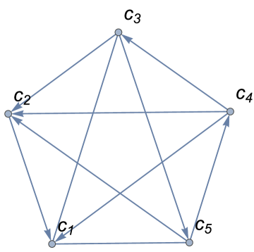
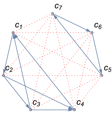
The PC matrix is skew-symmetric except the diagonal, so that for every $i,j=1,\ldots,n$ it holds that $m_{ij}+m_{ji}=0$ . An example of the ordinal PC matrix for five alternatives is given below (1).

M=\left(\begin{array}[]{ccccc}0&1&0&1&0\\ -1&0&1&1&1\\ 0&-1&0&1&-1\\ -1&-1&-1&0&1\\ 0&-1&1&-1&0\end{array}\right)

(1)

The PC matrix can be easily represented in the form of a graph.

Definition 2

A tournament graph (t-graph) with $n$ vertices is a pair $T=(V,E_{d})$ where $V=c_{1},\ldots,c_{n}$ is a set of vertices and $E_{d}\subset V^{2}$ is a set of ordered pairs called directed edges, so that for every two distinct vertices $c_{i}$ and $c_{j}$ either $(c_{i},c_{j})\in E_{d}$ or $(c_{j},c_{i})\in E_{d}$ .

Let us expand the definition of a tournament graph so that it can also model the collection of pairwise comparisons with ties.

Definition 3

The generalized tournament graph (gt-graph) with $n$ vertices is a triple $G=(V,E_{u},E_{d})$ where $V=c_{1},\ldots,c_{n}$ is a set of vertices, $E_{u}\subset 2^{V}$ is a set of unordered pairs called undirected edges, and $E_{d}\subset V^{2}$ is a set of ordered pairs called directed edges, so that for every two distinct vertices $c_{i}$ and $c_{j}$ either $(c_{i},c_{j})\in E_{d}$ or $(c_{j},c_{i})\in E_{d}$ or $\{c_{i},c_{j}\}\in E_{u}$ .

Wherever it increases the readability of the text the directed and undirected edges $(c_{i},c_{j})$ , $(c_{j},c_{i})$ , $\{c_{i},c_{j}\}$ between $c_{i},c_{j}\in V$ are denoted as $c_{i}\rightarrow c_{j},c_{j}\rightarrow c_{i}$ and $c_{i}-c_{j}$ correspondingly.

It is easy to see that every tournament graph can easily be extended to a generalized tournament graph where $E_{u}=\emptyset$ . Therefore, it will be assumed that every t-graph is also a gt-graph, but not reversely.

Definition 4

A family of t-graphs with $n$ vertices will be denoted as $\mathscr{T}_{n}^{t}$ , where $\mathscr{T}_{n}^{t}=\{(V,E_{d})\,\textit{ is a t-graph, where}\,\left|V\right|=n\}$ , and similarly, a family of gt-graphs with $n$ vertices will be denoted as $\mathscr{T}_{n}^{g}$ , where $\mathscr{T}_{n}^{g}=\{(V,E_{u},E_{d})\,\textit{ is a gt-graph, where}\,\left|V\right|=n\}$

It is obvious that for every $n>0$ it holds that $\mathscr{T}_{n}^{t}\subsetneq\mathscr{T}_{n}^{g}$ .

Definition 5

A family of gt-graphs with $n$ vertices and $m$ directed edges will be denoted as $\mathscr{T}_{n,m}^{g}=\{(V,E_{u},E_{d})\,\textit{ is a gt-graph, where}\,\left|V\right|=n\,\textit{and}\,\left|E_{d}\right|=m\}$

Definition 6

A gt-graph $G_{M}\in\mathscr{T}_{n}^{g}$ is said to correspond to the $n\times n$ ordinal PC matrix $M=[m_{ij}]$ if every directed edge $(c_{i},c_{j})\in E_{d}$ implies $m_{ji}=1$ and $m_{ij}=-1$ , and every undirected edge $\{c_{i},c_{j}\}\in E_{u}$ implies $m_{ij}=0$ .

Definition 7

All three mutually distinct vertices $t=\{c_{i},c_{k},c_{j}\}\subseteq V$ are said to be a triad. The vertex $c$ is said to be contained by a triad $t=\{c_{i},c_{k},c_{j}\}$ if $c\in t$ . A triad $t=\{c_{i},c_{k},c_{j}\}$ is said to be covered by the edge $(p,q)\in E_{d}$ if $p,q\in t$ .

Sometimes it will be more convenient to write a triad $t=\{c_{i},c_{k},c_{j}\}$ as the set of edges, e.g. $\{c_{i}\rightarrow c_{k},c_{k}\,\text{---}\,c_{j},c_{i}\,\text{---}\,c_{j}\}$ . However, both notations are equivalent, the latter one allows the reader to immediately identify the type of triad.

Definition 8

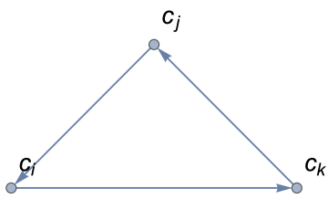
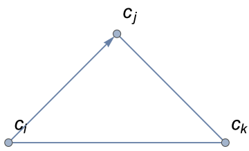
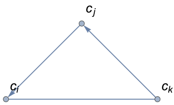
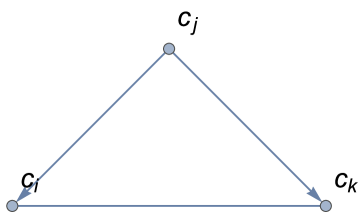
Refer to caption — Figure 1: The *gt-graph* corresponding to the matrix $M$ , see (1).

In their work, Kendall and Babington Smith dealt with the ordinal pairwise comparisons without ties [26]. Hence, in fact, they do not consider the situation in which $c_{i}\sim c_{j}$ . For the same reason, their ordinal PC matrices had no zeros anywhere outside the diagonal¹¹1In fact, those matrices had no zeros as the authors inserted dashes on the diagonal [26].. For the purpose of defining the notion of inconsistency in preferences, they adopt the transitivity of the preference relationship. According to this assumption, every triad $c_{i},c_{k},c_{j}$ of three different alternatives can be classified as consistent or inconsistent (contradictory). Providing that there are no ties between alternatives, there are two different kinds of triads (it is easy to verify that any other triad can be simply boiled down to one of these two by simple index changing). The first one $c_{i}\rightarrow c_{k},c_{k}\rightarrow c_{j}$ and $c_{i}\rightarrow c_{j}$ hereinafter referred to as the consistent triad²²2Index $3$ means that this kind of triad is formed by three directed edges. $\textit{CT}_{3}$ , and $c_{i}\rightarrow c_{k},c_{k}\rightarrow c_{j}$ and $c_{j}\rightarrow c_{i}$ termed hereinafter as the inconsistent triad $\textit{IT}_{3}$ (Fig. 2).

Of course, the more inconsistent the triads in the ordinal PC matrix, the more inconsistent the set of preferences, hence the less reliable the conclusions drawn from the set of paired comparisons. To determine how inconsistent the given set of paired comparisons is, Kendall and Babington Smith [26] provide the maximal number of inconsistent triads in the $n\times n$ PC matrix without ties. Denoting the actual number of inconsistent triads in $T_{M}$ by $\left|T_{M}\right|_{i}$ , and the maximal possible number of inconsistent triads in $n\times n$ PC matrix $M$ as $\mathcal{I}(n)$ , we have ³³3As every $n\times n$ ordinal PC matrix $M$ corresponds to some tournament graph $T_{n}^{\ast}$ we also use the notation $\left|T_{n}^{\ast}\right|_{i}$ to express the number of inconsistent triads in it.:

\mathcal{I}(n)=\left\{\begin{array}[]{ccc}\frac{n^{3}-n}{24}&\text{when}&\text{n is odd}\\ \frac{n^{3}-4n}{24}&\text{when}&\text{n is even}\end{array}\right.

(2)

Therefore, the inconsistency index for $M$ defined in [26] is:

\zeta(M)=1-\frac{\left|T_{M}\right|_{i}}{\mathcal{I}(n)}

(3)

Unfortunately, including ties into consideration significantly complicates the scene. Besides the two types of triads $\textit{CT}_{3}$ and $\textit{IT}_{3}$ we need to take into consideration an additional five:

$\textit{CT}_{0}$

- consistent triad of three equally preferred alternatives $c_{i},c_{k}$ and $c_{j}$ such that $c_{i}\sim c_{k},c_{k}\sim c_{j}$ and $c_{i}\sim c_{j}$ .
$\textit{IT}_{1}$

- inconsistent triad composed of three alternatives $c_{i},c_{k}$ and $c_{j}$ such that $c_{i}\sim c_{k},c_{k}\sim c_{j}$ and $c_{i}\prec c_{j}$ .
$\textit{IT}_{2}$

- inconsistent triad composed of three alternatives $c_{i},c_{k}$ and $c_{j}$ such that $c_{i}\sim c_{k},c_{k}\prec c_{j}$ and $c_{j}\prec c_{i}$ .
$\textit{CT}_{2a}$

- consistent triad composed of three alternatives $c_{i},c_{k}$ and $c_{j}$ such that $c_{i}\sim c_{k},c_{k}\prec c_{j}$ and $c_{i}\prec c_{j}$ .
$\textit{CT}_{2b}$

- consistent triad composed of three alternatives $c_{i},c_{k}$ and $c_{j}$ such that $c_{i}\sim c_{k},c_{j}\prec c_{k}$ and $c_{j}\prec c_{i}$ .

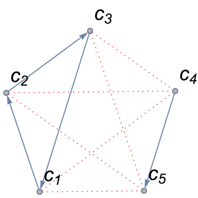
The above triads can be easily represented as tournament graphs with ties (Fig. 4). With the increased number of different types of triads in a graph, the maximum number of inconsistent triads also increases. For example, according to (2) the maximum number of inconsistent triads in $\mathcal{I}(4)$ without ties is $2$ . When ties are allowed, the maximal number of inconsistent triads increases to $4$ , which is the total number of triads in every simple graph (i.e. with only one edge between one pair of vertices) with four vertices.

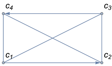
Let us analyze the graph in (Fig 3). It is easy to notice that it contains four $\textit{IT}_{1}$ triads which are: { $c_{1}\rightarrow c_{2},\,c_{2}\,\text{---}\,c_{3},\,c_{3}\,\text{---}\,c_{1}$ }, { $c_{1}\rightarrow c_{2},\,c_{2}\,\text{---}\,c_{4},\,c_{4}\,\text{---}\,c_{1}$ }, { $c_{1}\text{---}c_{3},\,c_{3}\,\rightarrow\,c_{4},\,c_{4}\,\text{---}\,c_{1}$ }, and { $c_{2}\,\text{---}\,c_{3},\,c_{3}\,\text{$\rightarrow$}\,c_{4},\,c_{4}\,\text{---}\,c_{1}$ }. Thus, it is clear that the formulae (2) and (3) cannot be used to estimate inconsistency in preferences when ties are allowed. The desire to extend those concepts to paired comparisons with ties was the main motivation for writing the work.

3 The most inconsistent set of preferences without ties

To construct the most inconsistent set of pairwise preferences without ties, let us introduce a few definitions relating to the degree of vertices. Since every t-graph is also a gt-graph the definitions are formulated for the gt-graph.

Definition 9

Let $G=(V,E_{u},E_{d})$ be a gt-graph and $c,d\in V$ . Then input degree, output degree, undirected degree and degree of a vertex $c$ are defined as follows: $\text{deg}_{\textit{in}}(c)\overset{\textit{df}}{=}\left|\{d\in V\,:\,d\rightarrow c\in E_{d}\}\right|$ , $\text{deg}_{out}(c)\overset{\textit{df}}{=}\left|\{d\in V\,:\,c\rightarrow d\in E_{d}\}\right|$ , $\text{deg}_{un}(c)\overset{\textit{df}}{=}\left|\{d\in V\,:\,c\,\text{---}\,d\in E_{u}\}\right|$ and $\text{deg}(c)\overset{\textit{df}}{=}\text{deg}_{\textit{in}}(c)+\text{deg}_{out}(c)+\text{deg}_{un}(c)$ .

Theorem 1

Let $G=(V,E_{u},E_{d})$ from $\mathscr{T}_{n}^{g}$ . Then every vertex $c\in V$ , for which $\text{deg}_{\textit{in}}(c)=k$ is contained by at least $\binom{k}{2}$ consistent triads of the type $\textit{CT}_{2a}$ or $\textit{CT}_{3}$ . Those triads are said to be introduced by $c$ .

Proof 1

Let $c_{1},\ldots,c_{k}\in V$ be the vertices such that the edges $c_{i}\rightarrow c$ are in $E_{d}$ . Since $T$ is a gt-graph with $n$ vertices, then for every $c_{i},c_{j}$ where $i,j=1,\ldots,k$ there must exist an edge $c_{i}\rightarrow c_{j}$ , $c_{j}\rightarrow c_{i}$ in $E_{d}$ or $c_{i}\,\text{---}\,c_{j}$ in $E_{u}$ . In the first two cases, the vertices $c_{i},c,c_{j}$ make a consistent triad type $\textit{CT}_{2a}$ , whilst in the latter case the vertices $c_{i},c,c_{j}$ form a consistent triad type $\textit{CT}_{3}$ . Since there are $k$ vertices adjacent via the incoming edge to $c$ there are at least as many different consistent triads containing $c$ as two-element combinations of $c_{1},\ldots,c_{k}$ i.e. $\binom{k}{2}$ . See (Fig. 5).

In general, the given vertex $c$ can form more consistent triads than those indicated in the above theorem. This is due to the fact that there may be two or more edges in the form $c\rightarrow c_{k+1},\dots,c\rightarrow c_{k+r}$ . Thus, in $T$ there may also be some number of consistent triads $\textit{CT}_{2b}$ containing $c$ .

The Theorem 1 is also true for the ordinary tournament graph (without ties). However, since the only consistent triads in such a graph are type $\textit{CT}_{3}$ (i.e. there are no triads of the type $\textit{CT}_{2a}$ or $\textit{CT}_{2b}$ containing $c$ ), the only consistent triads containing $c$ are those introduced by $c$ . This leads to the following observation:

Corollary 1

Let $T=(V,E_{d})$ from $\mathscr{T}_{n}^{t}$ . Then every vertex $c\in V$ , for which $\text{deg}_{in}(c)=k$ is contained by exactly $\binom{k}{2}$ consistent triads of the type $\textit{CT}_{3}$ .

Thus, if we would like to construct a tournament graph without ties which has the maximal number of inconsistent triads, we have to minimize the number of consistent triads introduced by the vertices, i.e.

\left|T\right|_{c}\overset{\textit{df}}{=}\sum_{c\in V}\binom{\text{deg}_{\textit{in}}(c)}{2}

(4)

Since there are no other consistent triads in the tournament graph than those introduced by the vertices, the expression (5) denotes, in fact, the number of inconsistent triads in some $T\in\mathscr{T}_{n}^{t}$ . Thus,

\left|T\right|_{i}=\binom{n}{3}-\sum_{c\in V}\binom{\text{deg}_{\textit{in}}(c)}{2}

(5)

It is commonly known that the sum of degrees in any undirected graph $G=(V,E)$ equals $2|E|$ [11, p. 5]. For the same reason in $T\in\mathscr{T}_{n}^{t}$ the sum of incoming edges into vertices is⁴⁴4Every directed edge corresponds to one victory. $|E|=\binom{n}{2}$ , i.e.:

\sum_{c\in V}\text{deg}_{\textit{in}}(c)=\binom{n}{2}

(6)

Hence, we would like to minimize (5) providing that the expression (6) holds. Intuitively $\left|T\right|_{i}$ is the largest (5) i.e. $\left|T\right|_{c}$ is the smallest (4) when the input degrees of vertices in a graph are the most evenly distributed⁵⁵5As it will be explained latter the input degrees are the most evenly distributed if for two different vertices $c,d$ holds that $\left|\deg_{\textit{in}}(c)-\deg_{\textit{in}}(d)\right|\leq 1$ . .

Definition 10

A gt-graph with $n$ vertices is said to be maximal with respect to the number of inconsistent triads, or briefly maximal if it has the highest possible number of inconsistent triads among the gt-graphs with the size $n$ . The fact that the gt-graph is maximal will be denoted $G\in\overline{\mathscr{T}_{n}^{g}}$ or $T\in\overline{\mathscr{T}_{n}^{t}}$ , depending on whether ties are or are not allowed. $\overline{\mathscr{T}_{n}^{t}}$ and $\overline{\mathscr{T}_{n}^{g}}$ denote families of gt-graphs with the highest possible number of inconsistent triads, i.e.

\overline{\mathscr{T}_{n}^{t}}=\{T\in\mathscr{T}_{n}^{t}\,\textit{such that}\,\left|T\right|_{i}=\underset{T_{r}\in\mathscr{T}_{n}^{t}}{\text{max}}\left|T_{r}\right|_{i}\}

(7)

\overline{\mathscr{T}_{n}^{g}}=\{G\in\mathscr{T}_{n}^{g}\,\textit{such that}\,\left|G\right|_{i}=\underset{G_{r}\in\mathscr{T}_{n}^{g}}{\text{max}}\left|G_{r}\right|_{i}\}

(8)

Before we prove the Theorem (2) about the maximal t-graph let us notice that for $r\in\mathbb{N}_{+}$ it holds that:

\binom{2r+1}{2}=r\cdot\left(2r+1\right)

(9)

and

\binom{2r}{2}=r\cdot r+r(r-1)

(10)

The above expression (9) means that by adopting $n=2r+1$ as the number of vertices in a graph, we may assign exactly $r$ incoming edges to every vertex $c$ in $V$ when $n$ is odd. Similarly (10), providing that $n=2r$ is even, we can assign $r$ incoming edges to $r$ vertices and $r-1$ incoming edges to the next $r$ vertices.

Theorem 2

The number of inconsistent triads in the t-graph $T=(V,E_{d})$ is maximal i.e. $T\in\overline{\mathscr{T}_{n}^{t}}$ if and only if

1.

for every $c$ in $V$ $\text{deg}_{\textit{in}}(c)=r$ when $n=2r+1$
2.

there are $r$ vertices $c_{1},\ldots,c_{r}$ in $V$ such that $\text{deg}_{\textit{in}}(c_{i})=r$ , and $r$ vertices $c_{r+1},\ldots,c_{n}$ such that $\text{deg}_{\textit{in}}(c_{j})=r-1$ , where $n=2r$ and $1\leq i\leq r<j\leq n$ .

Proof 2

To prove the theorem, it is enough to show that (4) is minimized by the distributions of the vertex degrees mentioned in the thesis of the theorem. Let us suppose that $n=2r+1$ and (4) is minimal but not all the vertices have input degrees equal $r$ . Thus, there must be at least one $c_{i}\in V$ such that $\text{deg}_{\textit{in}}(c_{i})\neq r$ . Let us suppose that $\text{deg}_{\textit{in}}(c_{i})=p>r$ (the second case is symmetric). Formulae (6) and (9) imply that there must also be at least one $c_{j}\in V$ such that $\text{deg}_{\textit{in}}(c_{j})=q<r$ . Therefore we can decrease $p$ and increase $q$ by one without changing the sum (6) just by replacing $c_{j}\rightarrow c_{i}$ to $c_{i}\rightarrow c_{j}$ . Since $p+q=z$ and $z$ is constant, the sum of consistent triads introduced by $c_{i}$ and $c_{j}$ (Theorem 1) is given as:

\binom{p}{2}+\binom{q}{2}=\binom{p}{2}+\binom{z-p}{2}=p(p-z)+\frac{z(z-1)}{2}

(11)

Since $z(z-1)/2$ is constant let

f(p)\overset{\textit{df}}{=}p(p-z)+\frac{z(z-1)}{2}

(12)

The value $f(p)$ decreases alongside a decreasing $p$ if

f(p)-f(p-1)>0

(13)

which is true if and only if

2p>(z-1)

(14)

Since $p>q$ and $p+q=z$ the last statement is true, which implies that, by decreasing $\text{deg}_{\textit{in}}(c_{i})$ and increasing $\text{deg}_{\textit{in}}(c_{j})$ by one, we can decrease the expression (4). This fact is contrary to the assumption that (4) is minimal, but not all the vertices have input degrees equal $r$ .

The proof for $n=2r$ is analogous to the case when $n=2r+1$ except the fact that as $c_{i}$ we should adopt such a vertex for which $\text{deg}_{\textit{in}}(c_{i})\neq r$ and $\text{deg}_{\textit{in}}(c_{i})\neq r-1$ . Note that there must be one if we reject the second statement of the thesis and, at the same time, we claim that (4) is minimal. \qed

The proof of (Theorem 2) also suggests an algorithm that converts any tournament graph into a graph with the maximal number of inconsistent triads. In every step of such an algorithm, it is enough to find a vertex $c_{i}$ whose input degree differs from $r$ (when $n$ is odd) or differs from $r$ and $r-1$ (when $n$ is even) and decreases (or increases) its input degree in parallel with increases (or decreases) in the input degree of $c_{j}$ . If it is impossible to find such a pair ( $c_{i},c_{j}$ ) this means that the graph is maximal. The algorithm satisfies the stop condition as with every iteration the number of inconsistent triads in a graph gets higher whilst the total number of triads in a graph is bounded by $\binom{n}{3}.$

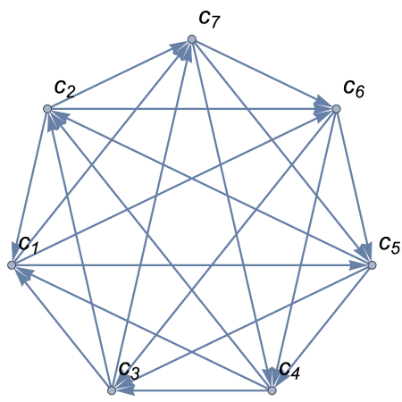
Kendall and Babington Smith [26] suggest a way of constructing the most inconsistent graph that brings to mind circulant graphs [33]. Namely, first add to a graph the cycle $c_{1}\rightarrow c_{2}\rightarrow c_{3}\rightarrow\ldots\rightarrow c_{n}\rightarrow c_{1}$ then the cycle $c_{1}\rightarrow c_{3}\rightarrow c_{5}\rightarrow\ldots\rightarrow c_{n}\rightarrow c_{2}\rightarrow\ldots$ if $n$ is even or two cycles $c_{1}\rightarrow c_{3}\rightarrow\ldots\rightarrow c_{n-1}\rightarrow c_{1}$ and $c_{2}\rightarrow c_{4}\rightarrow\ldots\rightarrow c_{n}\rightarrow c_{2}$ if $n$ is odd, and so on. Adding cycles with more and more skips needs to be continued until the insertion of all $\binom{n}{2}$ edges. An example of the maximally inconsistent graphs $T_{X}\in\mathscr{T}_{6}^{t}$ and $T_{Y}\in\mathscr{T}_{7}^{t}$ can be found in (Fig. 6). Those graphs correspond to the matrices $X$ and $Y$ (15).

X=\left(\begin{array}[]{cccccc}0&1&1&1&-1&-1\\ -1&0&1&1&1&-1\\ -1&-1&0&1&1&1\\ -1&-1&-1&0&1&1\\ 1&-1&-1&-1&0&1\\ 1&1&-1&-1&-1&0\end{array}\right)\,\,\,\,\,Y=\left(\begin{array}[]{ccccccc}0&1&1&1&-1&-1&-1\\ -1&0&1&1&1&-1&-1\\ -1&-1&0&1&1&1&-1\\ -1&-1&-1&0&1&1&1\\ 1&-1&-1&-1&0&1&1\\ 1&1&-1&-1&-1&0&1\\ 1&1&1&-1&-1&-1&0\end{array}\right)

(15)

The Theorem 2 clearly indicates the form of the most inconsistent tournament graph, but it does not specify the number of inconsistent triads in such a graph. This number, however, can be easily computed using the formula (2). To see that the results obtained so far are consistent with (2) as defined in [26] let us prove the following theorem.

Theorem 3

For every t-graph $T=(V,E_{d})$ where $T\in\overline{\mathscr{T}_{n}^{t}}$ , $n\geq 3$ which has the form defined by the Theorem 2 it holds that

\left|T\right|_{i}=\mathcal{I}(n)

(16)

Proof 3

According to (5)

\left|T\right|_{i}=\binom{2r+1}{3}-\sum_{c\in V}\binom{\text{deg}_{\textit{in}}(c)}{2}

(17)

Let $n=2r+1$ and $r\in\mathbb{N}_{+}$ . Then due to (Theorem 2)

\left|T\right|_{i}=\binom{2r+1}{3}-\underset{2r+1}{\left(\underbrace{\binom{r}{2}+\ldots+\binom{r}{2}}\right)}

(18)

\left|T\right|_{i}=\frac{r(2r-1)(2r+1)}{3}-\frac{(r-1)r(2r+1)}{2}

(19)

\left|T\right|_{i}=\frac{r\left(2r^{2}+3r+1\right)}{6}=\frac{(2r+1)^{3}-(2r+1)}{24}

(20)

\left|T\right|_{i}=\frac{(2r+1)^{3}-(2r+1)}{24}=\frac{n^{3}-n}{24}=\mathcal{I}(n)

(21)

Similarly, when $n=2r$ and $r\in\mathbb{N}_{+}$ . Then due to (Th. 2)

\left|T\right|_{i}=\binom{2r}{3}-\underset{r}{\left(\underbrace{\binom{r}{2}+\ldots+\binom{r}{2}}\right)}-\underset{r}{\left(\underbrace{\binom{r-1}{2}+\ldots+\binom{r-1}{2}}\right)}

(22)

\left|T\right|_{i}=\frac{r(2r-2)(2r-1)}{3}-\frac{(r-1)r^{2}}{2}-\frac{(r-2)(r-1)r}{2}

(23)

\left|T\right|_{i}=\frac{r\left(r^{2}-1\right)}{3}=\frac{(2r)^{3}-4(2r)}{24}=\frac{n^{3}-4n}{24}=\mathcal{I}(n)

(24)

which completes the proof of the theorem. \qed

The above theorem shows that the number of inconsistent triads in the tournament graph in which input degrees of their vertices are most evenly distributed is expressed by the formula provided by Kendall and Babington Smith [26]. This result, of course, is the natural consequence of the fact that such a graph is maximal as regards the number of inconsistent triads, as proven in (Theorem 2).

4 Properties of the most inconsistent set of preferences with ties

The graph representation of the set of paired comparisons with ties is the gt-graph. As it may contain two different types of edges, and hence, essentially more different kinds of triads (Fig. 4), the problem of finding the maximum number of inconsistent triads in such a graph is appropriately more difficult. The reasoning presented in this section is composed of three parts. In the first part, the properties of the gt-graph are discussed. Next, the maximally inconsistent gt-graph is proposed, and then, we prove that the proposed graph is indeed maximal with respect to the number of inconsistent triads.

The most straightforward example of the fully consistent gt-graph is a complete undirected graph of $n$ vertices (undirected $n$ -clique). It contains only undirected edges, thus all the triads contained in it are type $\textit{CT}_{0}$ . At first glance it seems that by successive replacing of undirected edges into directed ones we can make the graph more and more inconsistent. At the beginning, we will try to choose isolated edges i.e. those which are not adjacent to any directed edge. It is easy to observe that such edges alone cover $n-2$ different triads. Hence, by replacing isolated undirected edges into directed ones we increase the number of inconsistent triads by $n-2$ . Unfortunately, we can insert at most $\left\lfloor\frac{n}{2}\right\rfloor$ isolated directed edges (every isolated edge needs two vertices out of $n$ only for itself). Then we have to replace not isolated undirected edges into directed ones, and finally, we decide to make such replacements, which results in increasing the number of inconsistent triads in a graph, but also increases input degrees for some vertices. After several experiments carried out according to the above scheme, one may observe that it is not easy to choose the edge to replace. However, studying the above greedy algorithm is not useless. The first thing to notice is the fact that every gt-graph containing more than a certain number of edges should always have some number of consistent triads. Another finding is the observation that when constructing a maximal gt-graph one should strive to put at least one directed edge in each triad. Otherwise, the triad remains consistent, increasing the chance that the resulting gt-graph is not maximal. Both intuitive observations lead to the conclusion that the construction of the maximal gt-graph is a matter of finding a balance between too many directed edges resulting in the appearance of consistent triads of the type $\textit{CT}_{2a}$ and $\textit{CT}_{2b}$ and too few directed edges resulting in the existence of consistent triads of the type $\textit{CT}_{0}$ . Let us try to formulate this conclusion in a more formal way.

Theorem 4

Each gt-graph $G\in\mathscr{T}_{n,m}^{g}$ contains at least $\mathcal{C}(n,m)$ consistent triads of the type $\textit{CT}_{2a}$ or $\textit{CT}_{3}$ where

\mathcal{C}(n,m)=\frac{1}{2}\left\lfloor\frac{m}{n}\right\rfloor\left(2m-n\left\lfloor\frac{m}{n}\right\rfloor-n\right)

(25)

Proof 4

The theorem is a straightforward consequence of (Theorem 1 and 2). The first of them estimates the number of triads $\textit{CT}_{2a}$ or $\textit{CT}_{3}$ for a given vertex, whilst the second one shows that the sum of triads $\textit{CT}_{2a}$ or $\textit{CT}_{3}$ introduced by the vertices is minimal when the input degrees are evenly distributed. As we would like to determine the lower bound for the number of consistent triads in $G$ , we therefore have to assume that the input degrees are evenly distributed. Since there are $m$ directed edges in $G$ (it occurs that $m$ times one alternative is better than the other), then the sum of input degrees of vertices is $m$ . Therefore, adopting an even distribution postulate, every vertex has at least $\left\lfloor\frac{m}{n}\right\rfloor$ victories assigned (their input degree is at least $\left\lfloor\frac{m}{n}\right\rfloor$ ). Of course, the input degree of some of them may be larger by one. In other words, in the considered gt-graph there are $p$ vertices whose input degree is $\left\lfloor\frac{m}{n}\right\rfloor$ and $n-p$ vertices whose input degree might be $\left\lfloor\frac{m}{n}\right\rfloor+1$ . According to (Theorem 1) such a graph has at least $\mathcal{C}(n,m)$ consistent triads, where

\mathcal{C}(n,m)=p\binom{\left\lfloor\frac{m}{n}\right\rfloor}{2}+(n-p)\binom{\left\lfloor\frac{m}{n}\right\rfloor+1}{2}

(26)

We know that the sum of input degrees of vertices is $m$ , so

p\left\lfloor\frac{m}{n}\right\rfloor+(n-p)\left(\left\lfloor\frac{m}{n}\right\rfloor+1\right)=m

(27)

Hence,

p=n\left(\left\lfloor\frac{m}{n}\right\rfloor+1\right)-m

(28)

Therefore (26) can be written as

\mathcal{C}(n,m)=\left(n\cdot\left(\left\lfloor\frac{m}{n}\right\rfloor+1\right)-m\right)\cdot\binom{\left\lfloor\frac{m}{n}\right\rfloor}{2}+\left(m-n\cdot\left\lfloor\frac{m}{n}\right\rfloor\right)\cdot\binom{\left\lfloor\frac{m}{n}\right\rfloor+1}{2}

(29)

which, after appropriate transformations leads to (25). \qed

The immediate consequence of (Lemma 4) is the following corollary:

Corollary 2

Each gt-graph $G\in\mathscr{T}_{n,m}^{g}$ contains at most

\binom{n}{3}-\mathcal{C}(n,m)

(30)

inconsistent triads.

For the purpose of further consideration, let us denote by $\mathcal{T}$ a set of all the triads in the gt-graph and by $\mathcal{T}_{i}$ - a set of triads covered by $i=0,\ldots,3$ directed edges. For brevity, we denote the sum $\mathcal{T}_{i}\cup\mathcal{T}_{j}$ as $\mathcal{T}_{i,j}$ . In particular, it holds that $\mathcal{T}=\mathcal{T}_{0}\cup\mathcal{T}_{1}\cup\mathcal{T}_{2,3}$ . This allows the formulation of a quite straightforward but useful observation.

Corollary 3

As every two sets out of $\mathcal{T}_{0},\ldots,\mathcal{T}_{3}$ are mutually disjoint, then for every gt-graph $G\in\mathscr{T}_{n}^{g}$ it is true that

\binom{n}{3}=\left|\mathcal{T}_{0}\right|+\left|\mathcal{T}_{1}\right|+\left|\mathcal{T}_{2,3}\right|

(31)

Another important piece of information about the gt-graph follows from the number of undirected edges adjacent to particular vertices. Such edges may form the triads $\textit{CT}_{0}$ but may also form the triads $\textit{IT}_{1}$ (Fig. 7). This observation allows the number of both triad types to be estimated.

Lemma 1

For every gt-graph $G\in\mathscr{T}_{n}^{g}$ where $G=(V,E_{u},E_{d})$ it holds that

\sum_{c\in V}\binom{\text{deg}_{\textit{un}}(c)}{2}=3\left|\mathcal{T}_{0}\right|+\left|\mathcal{T}_{1}\right|

(32)

Proof 5

Let $c_{1}\,\text{---}\,c,\dots,c_{k}\,\text{---}\,c$ be the undirected edges in $E_{u}$ adjacent to some $c\in V$ . There are $\binom{k}{2}$ triads that contain $c$ . The type of triad depends on the edge $(c_{i},c_{j})$ . If $(c_{i},c_{j})\in E_{u}$ then the triad belongs to $\mathcal{T}_{0}$ whilst if $(c_{i},c_{j})\in E_{d}$ then the triad is in $\mathcal{T}_{1}$ . While calculating the sum $\sum_{c\in V}\binom{\text{deg}_{\textit{un}}(c)}{2}$ every uncovered triad is counted three times as there are three vertices adjacent to two undirected edges forming the triad. For the same reason, the triads covered by one directed edge are taken into account only once. \qed

Similarly as before, we try to generalize the result (32) to all the graphs that have $m$ directed edges.

Lemma 2

For each gt-graph $G\in\mathscr{T}_{n,m}^{g}$ where $G=(V,E_{u},E_{d})$ it holds that

\mathcal{D}(n,m)\leq 3\left|\mathcal{T}_{0}\right|+\left|\mathcal{T}_{1}\right|

(33)

where

\mathcal{D}(n,m)=\frac{1}{2}\left(n-\left\lfloor\frac{2m}{n}\right\rfloor-2\right)\left(n^{2}+n\left(\left\lfloor\frac{2m}{n}\right\rfloor-1\right)-4m\right)

(34)

Proof 6

Similarly as in (Lemma 4) the left side of (32) is minimal if undirected degrees are evenly distributed among the vertices. As for every $c\in V$ it holds that $\text{deg}_{\textit{un}}(c)=\text{deg}(c)-\text{deg}_{in}(c)-\text{deg}_{out}(c)$ then $\text{deg}_{\textit{un}}(c)=n-1-\left(\text{deg}_{in}(c)+\text{deg}_{out}(c)\right)$ . Thus, undirected degrees of vertices are evenly distributed if and only if the number of directed edges adjacent to the vertices are evenly distributed.

It is easy to see that in a gt-graph having $m$ directed edges the sum of input and output degrees is $2m$ . Thus, for every graph that minimizes the left side of (32) it holds that:

p\left\lfloor\frac{2m}{n}\right\rfloor+(n-p)\left(\left\lfloor\frac{2m}{n}\right\rfloor+1\right)=2m

(35)

The above equality means in particular that in such a graph there are $p\leq n$ vertices $c_{1},\ldots,c_{p}$ for which $\text{deg}_{\textit{in}}(c_{i})+\text{deg}_{out}(c_{i})=\left\lfloor\frac{2m}{n}\right\rfloor$ and $1\leq i\leq p$ , and $n-p$ vertices $c_{p+1},\ldots,c_{n}$ for which $\text{deg}_{\textit{in}}(c_{j})+\text{deg}_{out}(c_{j})=\left\lfloor\frac{2m}{n}\right\rfloor+1$ and $p+1\leq j\leq n$ . This statement also implies that in every graph that minimizes the left side of (32) there are $p$ vertices $c_{1},\ldots,c_{p}$ for which $\text{deg}_{un}(c_{i})=n-1-\left\lfloor\frac{2m}{n}\right\rfloor$ and $1\leq i\leq p$ , and also $n-p$ vertices $c_{p+1},\ldots,c_{n}$ for which $\text{deg}_{un}(c_{j})=n-2-\left\lfloor\frac{2m}{n}\right\rfloor$ and $p+1\leq j\leq n$ .

Thus, for every $G\in\mathscr{T}_{n,m}^{g}$ the lower bound of $3\left|\mathcal{T}_{0}\right|+\left|\mathcal{T}_{1}\right|$ is:

\mathcal{D}(n,m)=p\binom{n-1-\left\lfloor\frac{2m}{n}\right\rfloor}{2}+(n-p)\binom{n-2-\left\lfloor\frac{2m}{n}\right\rfloor}{2}

(36)

Since from (35) $p$ equals

p=n\left(\left\lfloor\frac{2m}{n}\right\rfloor+1\right)-2m

(37)

Thus,

	$\displaystyle\mathcal{D}(n,m)=$	$\displaystyle\left(n\left(\left\lfloor\frac{2m}{n}\right\rfloor+1\right)-2m\right)\binom{n-1-\left\lfloor\frac{2m}{n}\right\rfloor}{2}$
		$\displaystyle+\left(2m-n\left\lfloor\frac{2m}{n}\right\rfloor\right)\binom{n-2-\left\lfloor\frac{2m}{n}\right\rfloor}{2}$		(38)

The above expression simplifies to

\mathcal{D}(n,m)=\frac{1}{2}\left(-\left\lfloor\frac{2m}{n}\right\rfloor+n-2\right)\left(n\left\lfloor\frac{2m}{n}\right\rfloor-4m+(n-1)n\right)

(39)

which completes the proof of the theorem. \qed

Through the analysis of the degree of vertices we can also estimate the value $\left|\mathcal{T}_{2,3}\right|$ .

Lemma 3

For every gt-graph $G\in\mathscr{T}_{n}^{g}$ where $G=(V,E_{u},E_{d})$ it holds that

\frac{1}{3}\sum_{c\in V}\binom{\text{deg}_{\textit{in}}(c)+\text{deg}_{out}(c)}{2}\leq\left|\mathcal{T}_{2,3}\right|

(40)

Proof 7

Let $c_{1}\rightarrow c,c\rightarrow c_{2},\dots,c_{k}\rightarrow c$ be the directed edges in $E_{d}$ adjacent to some $c\in V$ . There are $\binom{k}{2}$ triads that contain $c$ where $k=\text{deg}_{\textit{in}}(c)+\text{deg}_{\textit{out}}(c)$ , which are covered by two or three directed edges. While calculating the sum $\sum_{c\in V}\binom{\text{deg}_{\textit{in}}(c)+\text{deg}_{\textit{out}}(c)}{2}$ triads covered by two directed edges are counted once, whilst all the triads covered by three directed edges are counted three times. In the worst case scenario, all the considered triads are covered by three directed edges. Thus, $\frac{1}{3}\sum_{c\in V}\binom{\text{deg}_{\textit{in}}(c)+\text{deg}_{\textit{out}}(c)}{2}$ is the lower bound for $\left|\mathcal{T}_{2,3}\right|$ . This observation completes the proof. \qed

Similarly as before, let us extend the above Lemma to all gt-graphs that have $n$ vertices and $m$ directed edges.

Lemma 4

For each gt-graph $G\in\mathscr{T}_{n,m}^{g}$ where $G=(V,E_{u},E_{d})$ it holds that

\mathcal{E}(n,m)\leq\left|\mathcal{T}_{2,3}\right|

(41)

where

\mathcal{E}(n,m)=\frac{1}{6}\left\lfloor\frac{2m}{n}\right\rfloor\left(4m-n\left(\left\lfloor\frac{2m}{n}\right\rfloor+1\right)\right)

(42)

Proof 8

Similarly as in (Lemma 2) the left side of (40) is minimal if the sum of input and output degrees of the vertices are evenly distributed. It is easy to see that in a gt-graph that has $m$ directed edges the sum of input and output degrees is $2m$ . Thus, for every graph that minimizes the left side of (40) it holds that (35). This implies that in the gt-graph which minimizes the left side of (40) there should be $p$ vertices adjacent to $\left\lfloor\frac{2m}{n}\right\rfloor$ directed edges and $n-p$ vertices adjacent to $\left\lfloor\frac{2m}{n}\right\rfloor+1$ directed edges. Based on (40) we conclude that

\mathcal{E}(n,m)=\frac{1}{3}\left(p\binom{\left\lfloor\frac{2m}{n}\right\rfloor}{2}+\left(n-p\right)\binom{\left\lfloor\frac{2m}{n}\right\rfloor+1}{2}\right)

(43)

Applying (37) we obtain

	$\displaystyle\mathcal{E}(n,m)=$	$\displaystyle\frac{1}{3}\left\{\left[n\left(\left\lfloor\frac{2m}{n}\right\rfloor+1\right)-2m\right]\binom{\left\lfloor\frac{2m}{n}\right\rfloor}{2}\right.$
		$\displaystyle+\left.\left[n-\left(n\left(\left\lfloor\frac{2m}{n}\right\rfloor+1\right)-2m\right)\right]\binom{\left\lfloor\frac{2m}{n}\right\rfloor+1}{2}\right\}$		(44)

Hence,

\mathcal{E}(n,m)=\frac{1}{3}\left\{\left(n\left\lfloor\frac{2m}{n}\right\rfloor+n-2m\right)\binom{\left\lfloor\frac{2m}{n}\right\rfloor}{2}\right.\left.+\left(2m-n\left\lfloor\frac{2m}{n}\right\rfloor\right)\binom{\left\lfloor\frac{2m}{n}\right\rfloor+1}{2}\right\}

(45)

The above equation simplifies to

\mathcal{E}(n,m)=\frac{1}{6}\left\lfloor\frac{2m}{n}\right\rfloor\left(4m-n\left\lfloor\frac{2m}{n}\right\rfloor-n\right)

(46)

Which completes the proof of the Lemma. \qed

The Corollary (3) and Lemmas (1 - 4) allow us to estimate the minimal number of consistent triads which are not covered by any directed edge.

Theorem 5

For each gt-graph $G\in\mathscr{T}_{n,m}^{g}$ where $G=(V,E_{u},E_{d})$ holds that

\mathcal{F}(n,m)\leq\left|\mathcal{T}_{0}\right|

(47)

where

\mathcal{F}(n,m)=\frac{1}{2}\left(\mathcal{D}(n,m)+\mathcal{E}(n,m)-\binom{n}{3}\right)

(48)

which is equivalent to

\mathcal{F}(n,m)=\frac{1}{6}\left(-2n\left\lfloor\frac{2m}{n}\right\rfloor^{2}+(8m-2n)\left\lfloor\frac{2m}{n}\right\rfloor+(n-2)((n-1)n-6m)\right)

(49)

Proof 9

According to (Corollary 3)

\binom{n}{3}=\left|\mathcal{T}_{0}\right|+\left|\mathcal{T}_{1}\right|+\left|\mathcal{T}_{2,3}\right|

(50)

Due to (Lemma 2) it holds that

\mathcal{D}(n,m)-3\left|\mathcal{T}_{0}\right|\leq\left|\mathcal{T}_{1}\right|

(51)

Therefore it is true that

\binom{n}{3}\geq\left|\mathcal{T}_{0}\right|+\left(\mathcal{D}(n,m)-3\left|\mathcal{T}_{0}\right|\right)+\left|\mathcal{T}_{2,3}\right|=\mathcal{D}(n,m)+\left|\mathcal{T}_{2,3}\right|-2\left|\mathcal{T}_{0}\right|

(52)

As we know (Lemma 4) that $\mathcal{E}(n,m)\leq\left|\mathcal{T}_{2,3}\right|$ it is true that

\binom{n}{3}\geq\mathcal{D}(n,m)+\mathcal{E}(n,m)-2\left|\mathcal{T}_{0}\right|

(53)

Hence,

\left|\mathcal{T}_{0}\right|\geq\frac{1}{2}\left(\mathcal{D}(n,m)+\mathcal{E}(n,m)-\binom{n}{3}\right)

(54)

which, after simplifying, leads to

\left|\mathcal{T}_{0}\right|\geq\frac{1}{6}\left((8m-2n)\left\lfloor\frac{2m}{n}\right\rfloor-2n\left\lfloor\frac{2m}{n}\right\rfloor^{2}+(n-2)((n-1)n-6m)\right)

(55)

Which completes the proof of the theorem. \qed

One can easily check that for fixed $n$ the values of $\mathcal{F}(n,m)$ decrease to $0$ then become negative, whilst $\left|\mathcal{T}_{0}\right|$ is always a positive integer. Hence, the inequality (47) can also be written as:

\max\{0,\left\lceil\mathcal{F}(n,m)\right\rceil\}\leq\left|\mathcal{T}_{0}\right|

(56)

Both theorems 4 and 5 provide estimations for the minimal number of consistent triads in a gt-graph. Theorem 4 provides the lower bound $\mathcal{C}(n,m)$ for the number of triads $\textit{CT}_{2a}$ and $\textit{CT}_{3}$ , whilst Theorem 5 provides the lower bound for the number of consistent triads $\textit{CT}_{0}$ . Hence, the number of consistent triads in the gt-graph $T\in\mathscr{T}_{n,m}^{g}$ cannot be lower than $\mathcal{G}(n,m)$ where

\mathcal{G}(n,m)\stackrel{{\scriptstyle\textit{df}}}{{=}}\mathcal{C}(n,m)+\max\{0,\left\lceil\mathcal{F}(n,m)\right\rceil\}

(57)

Of course, its number could be even higher as we do not care about triads $\textit{CT}_{2b}$ . The immediate consequence of the above expression is the observation that the number of inconsistent triads in the gt-graph cannot be higher than $\mathcal{H}(n,m)$ where:

\mathcal{H}(n,m)\stackrel{{\scriptstyle\textit{df}}}{{=}}\binom{n}{3}-\mathcal{G}(n,m)

(58)

In particular, the most inconsistent gt-graph $G\in\overline{\mathscr{T}_{n}^{g}}$ with some fixed $n\geq 3$ can have as many inconsistent triads as the maximal value of the upper bounding function $\mathcal{H}(n,m)$ , i.e.

\left|G\right|_{i}\leq\max_{0\leq m\leq\binom{n}{2}}\mathcal{H}(n,m)

(59)

Reversely, a gt-graph $G\in\mathscr{T}_{n}^{g}$ , which fits that maximum must be maximal i.e. wherever $\left|G\right|_{i}=\max_{0\leq m\leq\binom{n}{2}}\mathcal{H}(n,m)$ then $G\in\overline{\mathscr{T}_{n}^{g}}$ . Through the experimental analysis of the upper bounding function $\mathcal{H}(n,m)$ we can see that for every fixed $n$ it has one distinct maximum (Fig. 8).

In the next section we propose the graph which fits the maximum of $\mathcal{H}(n,m)$ and formally prove indispensable theorems.

5 The most inconsistent set of preferences with ties

In order to find the maximal gt-graph, let us try to look at the function $\mathcal{H}(n,m)$ and the two functions $\mathcal{C}(n,m)$ and $\mathcal{F}(n,m)$ of which it is composed (Fig. 9). $\mathcal{C}(n,m)$ determines the minimal number of consistent triads covered by more than one directed edge. The more directed edges, the greater the number of consistent triads in a graph. Hence, for some small number of directed edges $\mathcal{C}$ equals $0$ , then slowly begins to grow. The function $\mathcal{F}(n,m)$ indicates the minimal number of triads not covered by any directed edge. Those triads are also consistent. With the increase in the number of directed edges, their quantity decreases and eventually reaches $0$ . Since for the positive ordinates $\mathcal{F}$ decreases faster than $\mathcal{C}$ grows, then the function $\mathcal{H}$ reaches the maximum when $\mathcal{F}$ becomes $0$ . This indicates that in the optimal gt-graph all the triads should be covered by at least one directed edge. This requires the introduction of so many directed edges that the number of triads will become consistent thereby. 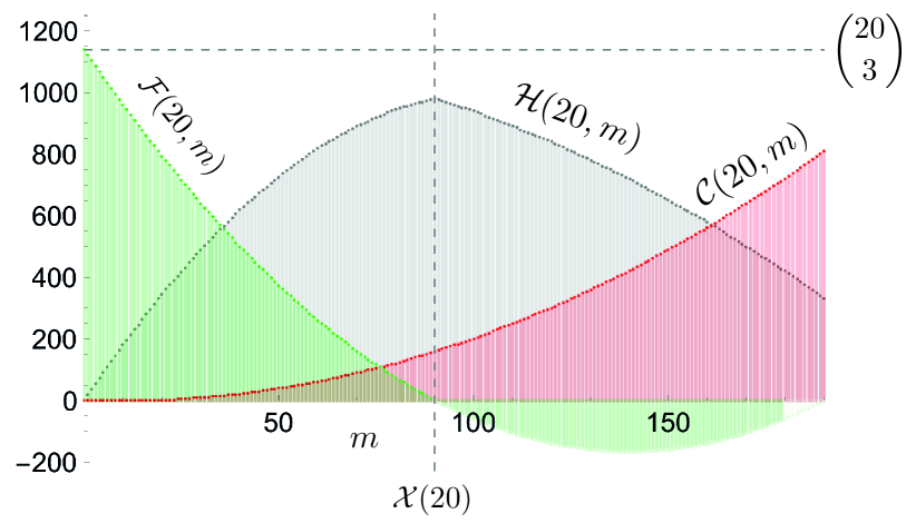However, the slope of both functions $\mathcal{F}$ and $\mathcal{C}$ indicates that it is more important to cover each triad $\textit{CT}_{0}$ than not to create too many consistent triads $\textit{CT}_{2a},\textit{CT}_{2b}$ or $\textit{CT}_{3}$ .

The considerations in the previous section also indicate that directed edges should be evenly distributed. Otherwise, the gt-graph may not be maximal. The above somewhat intuitive considerations, based on the viewing functions in the figure, lead to the definition of the most inconsistent gt-graph.

Definition 11

A double tournament graph (hereinafter referred to as dt-graph), is a gt-graph $G=(V_{1}\cup V_{2},E_{d_{1}}\cup E_{d_{2}},E_{u})$ such that $(V_{1},E_{d_{1}})$ and $(V_{2},E_{d_{2}})$ are t-graphs, where $V_{1}\cap V_{2}=\emptyset$ and $E_{u}=\{\{c,d\}\,\,:\,\,c\in V_{1}\,\wedge\,d\in V_{2}\}$ .

It is easy to observe that in every dt-graph all triads are covered by directed edges (Lemma 6). Thus, for every dt-graph it holds that $\max\{0,\left\lceil\mathcal{F}(n,m)\right\rceil\}=0$ . This does not guarantee, however, the minimality of $\mathcal{C}(n,m)$ . Let us propose an improved version of the dt-graph, which, as will be shown later, indeed contains the maximal number of inconsistent triads.

Proposition 1

The dt-graph $T=(V_{1}\cup V_{2},E_{d_{1}}\cup E_{d_{2}},E_{u})$ is the maximal dt-graph if $(V_{1},E_{d_{1}})$ and $(V_{2},E_{d_{2}})$ are maximal t-graphs where $\left|V_{1}\right|=\left\lfloor\frac{n}{2}\right\rfloor$ and $\left|V_{2}\right|=\left\lceil\frac{n}{2}\right\rceil$ .

In other words, we suppose that the dt-graph with $n$ vertices composed of two maximal t-graphs whose numbers of vertices are identical (when $n$ is even) or differ by one (when $n$ is odd) is maximal. Examples of such maximal dt-graph candidates can be found at (Fig. 10). The matrices that correspond to the graphs $G_{X^{*}}$ and $G_{Y^{*}}$ are given as (60).

X^{*}=\left(\begin{array}[]{cccccc}0&-1&1&0&0&0\\ 1&0&-1&0&0&0\\ -1&1&0&0&0&0\\ 0&0&0&0&-1&1\\ 0&0&0&1&0&-1\\ 0&0&0&-1&1&0\end{array}\right)\,\,\,\,Y^{*}=\left(\begin{array}[]{ccccccc}0&-1&1&1&0&0&0\\ 1&0&-1&-1&0&0&0\\ -1&1&0&-1&0&0&0\\ -1&1&1&0&0&0&0\\ 0&0&0&0&0&1&-1\\ 0&0&0&0&-1&0&1\\ 0&0&0&0&1&-1&0\end{array}\right)

(60)

Let us denote the number of directed edges in a maximal dt-graph candidate by $\mathcal{X}(n)$ . It is easy to see that:

\mathcal{X}(n)=\binom{\left\lfloor\frac{n}{2}\right\rfloor}{2}+\binom{\left\lceil\frac{n}{2}\right\rceil}{2}

(61)

Corollary 4

It can be easily calculated that when $n$ is even i.e. $n=2q$ and $q\in\mathbb{N}_{+}$ it holds that

\mathcal{X}(2q)=q(q-1)

(62)

whilst when $n$ is odd i.e. $n=2q+1$ and $q\in\mathbb{N}_{+}$ it holds that

\mathcal{X}(2q+1)=q^{2}

(63)

To determine the number of consistent/inconsistent triads in this “maximal gt-graph candidate” let us observe that all the consistent triads are in the two maximal tournament subgraphs. This observation can be written in the form of a short Lemma.

Lemma 5

For every dt-graph $G=(V_{1}\cup V_{2},E_{d_{1}}\cup E_{d_{2}},E_{u})$ and a triad $t=\{v_{i},v_{k},v_{j}\}$ if $t\cap V_{1}\neq\emptyset$ and $t\cap V_{2}\neq\emptyset$ then $t$ is inconsistent.

Proof 10

Since $t\cap V_{1}\neq\emptyset$ and $t\cap V_{2}\neq\emptyset$ , there are two vertices from $t$ in one of the two sets $V_{1}$ and $V_{2}$ and one vertex from $t$ in the other set. Let us suppose that $v_{i},v_{k}\in V_{1}$ and $v_{j}\in V_{2}$ . Since $(V_{1},E_{d_{1}})$ is a t-graph then the edge between $v_{i}$ and $v_{k}$ is directed. Due to the definition of dt-graph both edges $(v_{i},v_{j})$ and $(v_{k},v_{j})$ are undirected, hence $t$ is $IT_{1}$ . \qed

The immediate conclusion can be written as the Lemma

Lemma 6

The dt-graph does not contain uncovered triads

Proof 11

Let us consider the dt-graph $G=(V_{1}\cup V_{2},E_{d_{1}}\cup E_{d_{2}},E_{u})$ and a triad $t=\{v_{i},v_{k},v_{j}\}$ . If $v_{i},v_{k}\in V_{1}$ and $v_{j}\in V_{2}$ then $t$ is inconsistent (Lemma 5), hence it cannot be uncovered. If all $v_{i},v_{k},v_{j}\in V_{1}$ then all three edges are spanned between $v_{i},v_{k}$ and $v_{j}$ . Hence, $t$ is covered. The proof is completed as all the other cases are similar. \qed

It is also easy to determine the number of inconsistent triads in the candidate graph. Due to (Theorem 3) the number of consistent triads in the maximal tournament sub-graphs are $\binom{\left\lfloor\frac{n}{2}\right\rfloor}{3}-\mathcal{I}\left(\left\lfloor\frac{n}{2}\right\rfloor\right)$ and $\binom{\left\lceil\frac{n}{2}\right\rceil}{3}-\mathcal{I}\left(\left\lceil\frac{n}{2}\right\rceil\right)$ correspondingly. Since there are no consistent triads in double tournament graphs, except those that are fully enclosed in the maximal tournament sub-graphs (Lemma 5), the number of inconsistent triads in the maximal gt-graph candidate is given as:

\mathcal{Y}(n)=\binom{n}{3}-\left(\binom{\left\lfloor\frac{n}{2}\right\rfloor}{3}-\mathcal{I}\left(\left\lfloor\frac{n}{2}\right\rfloor\right)\right)-\left(\binom{\left\lceil\frac{n}{2}\right\rceil}{3}-\mathcal{I}\left(\left\lceil\frac{n}{2}\right\rceil\right)\right)

(64)

To confirm that a dt-graph (Proposition 1) is indeed maximal we need to prove that

1.

the function $\mathcal{H}(n,m)$ reaches the maximum when the number of directed edges in a graph equals $m=\mathcal{X}(n)$ , and
2.

the maximum of $\mathcal{H}(n,m)$ equals $\mathcal{Y}(n)$

Therefore to make the Proposition 1 a fully fledged claim we prove (Theorem 6). However, before we start (Theorem 6) let us prove a couple of Lemmas which formally confirm what we have seen at (Fig. 9). The aim of the first Lemma (7) is a formal confirmation of the shape of the function $\mathcal{F}$ . In particular, it confirms that $\mathcal{F}$ crosses the x-axis at the same point where $\mathcal{H}$ reaches the maximum i.e. for every fixed $n\geq 3$ , $\mathcal{F}$ is positive when $0\leq m<\mathcal{X}(n)$ , equals $0$ when $m=\mathcal{X}(n)$ and it is non-positive for $\mathcal{X}(n)\leq m\leq\binom{n}{2}$ .

Lemma 7

For every $n\in\mathbb{N}_{+},n\geq 3$ and $k\in\mathbb{N}_{+}$ it holds that:

\mathcal{F}(n,\mathcal{X}(n))=0

(65)

\mathcal{F}(n,\mathcal{X}(n)-k)\geq 1,\,\,\,\text{where}\,\,\,0<k<\mathcal{X}(n)

(66)

\mathcal{F}(n,\mathcal{X}(n)+k)\leq 0,\,\,\,\text{where}\,\,\,0<k\leq\binom{n}{2}-\mathcal{X}(n)

(67)

Proof 12

Proof of the Lemma, consisting of elementary but time consuming operations, can be found in (A).

The aim of the next Lemma is to show that $\mathcal{C}$ is strictly increasing for every $m$ not smaller than $n$ and obviously not greater than the maximal number of edges in a gt-graph i.e. $\binom{n}{2}$ (Fig. 9). Thus, by adding more directed edges than $n$ we may only increase the minimal number of consistent triads of the types $\textit{CT}_{2a}$ or $\textit{CT}_{3}$ .

Lemma 8

For every $n\in\mathbb{N}_{+},n\geq 3$ the function $\mathcal{C}$

1.

is constant and equals $\mathcal{C}(n,m)=0$ for every $m$ such that $0\leq m<n$
2.

is strictly increasing for every $m\in\mathbb{N}_{+}$ such that $n\leq m\leq\binom{n}{2}$ , i.e.

$\mathcal{C}(n,m+1)-\mathcal{C}(n,m)>0$ (68)

Proof 13

Proof of the Lemma, consisting of elementary but time consuming operations, can be found in (B).

In every gt-graph with $n$ vertices and $m$ directed edges there are at least $\mathcal{C}(n,m)$ consistent triads $\textit{CT}_{2a}$ or $\textit{CT}_{3}$ . This means that in this graph there are at most $\binom{n}{3}-\mathcal{C}(n,m)$ inconsistent triads. In particular the Lemma 9 shows that there is no gt-graph with $n$ vertices and $\mathcal{X}(n)$ directed edges which has more inconsistent triads than the maximal gt-graph defined in (Proposition 1).

Lemma 9

For every $n\in\mathbb{N}_{+},n\geq 3$ it holds that

\mathcal{Y}(n)=\binom{n}{3}-\mathcal{C}(n,\mathcal{X}(n))

(69)

Proof 14

Proof of the Lemma, composed of elementary but time consuming operations, can be found in (C).

The next Lemma shows that the minimal number of consistent triads in a gt-graph decreases along with adding the next directed edges. Such a decrease continues as long as the number of directed edges does not reach the value $\mathcal{X}(n)$ . In other words, following the increasing number of directed edges (until there are less than $\mathcal{X}(n)$ ) the number of inconsistent triads also increases.

Lemma 10

For every $n\in\mathbb{N}_{+},n\geq 3$ the function $\mathcal{G}$ is strictly decreasing for every $m\in\mathbb{N}_{+}$ such that $1\leq m\leq\mathcal{X}(n)$ , i.e.

\mathcal{G}(n,m)-\mathcal{G}(n,m+1)>0\,\,\,\textit{where}\,\,\,1\leq m<\mathcal{X}(n)

(70)

Proof 15

Proof of the Lemma, composed of elementary but time consuming operations, can be found in (D).

For every fixed $n\geq 3$ the function $\mathcal{H}$ determines the maximal possible number of inconsistent triads in every gt-graph.

The aim of the theorem below is to confirm that, indeed, the proposed dt-graph (Proposition 1) is a maximal gt-graph.

Theorem 6

For every dt-graph $G=(V_{1}\cup V_{2},E_{d_{1}}\cup E_{d_{2}},E_{u})$ with $n$ vertices where $(V_{1},E_{d_{1}})$ and $(V_{2},E_{d_{2}})$ are maximal t-graphs and $\left|V_{1}\right|=\left\lfloor\frac{n}{2}\right\rfloor$ and $\left|V_{2}\right|=\left\lceil\frac{n}{2}\right\rceil$ and $n>3$ it holds that:

1.

$\mathcal{X}(n)=m$ maximizes $\mathcal{H}(n,m)$ , i.e.

$\mathcal{H}(n,\mathcal{X}(n))=\max_{0\leq m\leq\binom{n}{2}}\mathcal{H}(n,m)$ (71)
2.

$\mathcal{Y}(n)$ is a maximum of $\mathcal{H}(n,m)$

$\mathcal{H}(n,\mathcal{X}(n))=\mathcal{Y}(n)$ (72)

Proof 16

As (58) then the first claim of the theorem is equivalent to

\mathcal{G}(n,\mathcal{X}(n))=\min_{0\leq m\leq\binom{n}{2}}\mathcal{G}(n,m)

(73)

As (57) then the function $\mathcal{G}$ is the sum of $\mathcal{C}(n,m)$ and $\max\{0,\left\lceil\mathcal{F}(n,m)\right\rceil\}$ . From (Lemma 8) we know that $\mathcal{C}$ does not decrease with respect to $m$ . On the other hand, due to the (Lemma 7) $\mathcal{F}(n,\mathcal{X}(n)+k)\leq 0$ for every $0<k\leq\binom{n}{2}-\mathcal{X}(n)$ , which translates to the observation that for every $m\geq\mathcal{X}(n)$ it holds that $\max\{0,\left\lceil\mathcal{F}(n,m)\right\rceil\}=0$ . Hence, for every $m\geq\mathcal{X}(n)$ the function $\mathcal{G}$ does not decrease and boils down to $\mathcal{G}(n,m)=\mathcal{C}(n,m)$ . In other words

\mathcal{G}(n,\mathcal{X}(n))\leq\mathcal{G}(n,\mathcal{X}(n)+1)\leq\ldots\leq\mathcal{G}(n,\binom{n}{2})

(74)

This fact, coupled with (Lemma 10) i.e.

\mathcal{G}(n,0)>\mathcal{G}(n,1)>\ldots>\mathcal{G}(n,\mathcal{X}(n))

(75)

implies that indeed

\mathcal{G}(n,\mathcal{X}(n))=\min_{0\leq m\leq\binom{n}{2}}\mathcal{G}(n,m)

(76)

which completes the proof of the first claim (71) of the Theorem 6. To prove the second claim it is enough to recall that for every $m\geq\mathcal{X}(n)$ it holds that $\mathcal{G}(n,m)=\mathcal{C}(n,m)$ . Thus, in particular

\mathcal{H}(n,\mathcal{X}(n))=\binom{n}{3}-\mathcal{C}(n,\mathcal{X}(n))

(77)

which satisfies the second claim (72) of the Theorem 6, and which thereby confirms the Proposition 1. \qed

6 Inconsistency indices in paired comparisons with ties

As shown in (Section 2) the inconsistency index (called there “coefficient of consistence”) defined by Kendall and Babington Smith [26, p. 330] cannot be used in the context of ordinal pairwise comparisons with ties. Thus, in (3) $\mathcal{I}(n)$ needs to be replaced by $\mathcal{Y}(n)$ - the maximal number of triads in the case when ties are allowed. The generalized inconsistency index that covers pairwise comparisons with ties finally takes the form

\zeta_{g}(M)=1-\frac{\left|G_{M}\right|_{i}}{\mathcal{Y}(n)}

(78)

where $M$ is an ordinal PC matrix with ties of the size $n\times n$ (Def. 1) and G is a gt-graph corresponding to $M$ . The formula (78), although concise, may not be handy in practice. This is due to the use in (64) of the floor $\left\lfloor x\right\rfloor$ and ceiling $\left\lceil x\right\rceil$ operations as well as binomial symbol $\binom{x}{y}$ . For this reason, let us simplify (64) depending on whether $n$ and $\nicefrac{{n}}{{2}}$ are odd or even. There are four cases that need to be considered:

\mathcal{Y}(n)=\begin{cases}\frac{13n^{3}-24n^{2}-16n}{96}&\text{when}\,\,\,n=4q\,\,\,\text{for}\,\,\,q=1,2,3,\ldots\\ \frac{13n^{3}-24n^{2}-19n+30}{96}&\text{when}\,\,\,n=4q+1\,\,\,\text{for}\,\,\,q=1,2,3,\ldots\\ \frac{13n^{3}-24n^{2}-4n}{96}&\text{when}\,\,\,n=4q+2\,\,\,\text{for}\,\,\,q=1,2,3,\ldots\\ \frac{13n^{3}-24n^{2}-19n+18}{96}&\text{when}\,\,\,n=4q+3\,\,\,\text{for}\,\,\,q=0,1,2,\ldots\end{cases}

(79)

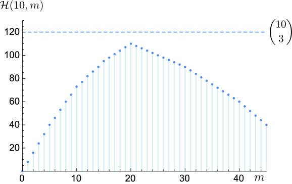
For example, to compute the inconsistency index for the ordinal PC matrix $M$ (1) (see Fig. 1) first it is necessary to compute the number of inconsistent triads in $M$ . Since (1) has five inconsistent triads: $(A_{1},A_{2},A_{3})$ , $(A_{1},A_{2},A_{5})$ , $(A_{1},A_{3},A_{5})$ , $(A_{1},A_{4},A_{5})$ and $(A_{3},A_{4},A_{5})$ then $\left|T_{M}\right|=5$ . On the other hand, $5=4\cdot 1+1$ hence, the value $\mathcal{Y}(5)$ is obtained by replacing $n$ with $5$ in the expression $\nicefrac{{1}}{{96}}\cdot\left(13n^{3}-24n^{2}-19n+30\right)$ , i.e. $\mathcal{Y}(5)=10$ . In other words, in the considered gt-graph (Fig. 1) five triads out of ten possible ones are inconsistent. The generalized consistency index for $M$ takes the form:

\zeta_{g}(M)=1-\frac{5}{10}=\frac{1}{2}

(80)

Hence the inconsistency level for $M$ (1) is $50\%$ .

As every t-graph is also a gt-graph but not reversely (see Def. 2 and 3) then the generalized inconsistency index $\zeta_{g}$ can also be used to estimate the inconsistency level of paired comparisons without ties. Conversely it is not possible.

Both inconsistency indices $\zeta$ and $\zeta_{g}$ compare the number of inconsistent triads in $M$ with the maximal number of such triads in a matrix of the same size as $M$ . Hence, for the maximally inconsistent matrix the index functions will return $1$ , whilst the inconsistency index for a fully consistent matrix is $0$ . The maximal value of the inconsistency index, of course, does not automatically imply that all the triads in the given matrix are inconsistent. To capture this phenomenon, let us define the absolute inconsistency index $\eta$ as a ratio of the number of inconsistent triads to the number of all possible triads in the $n\times n$ matrix $M$ .

\eta(M)\stackrel{{\scriptstyle\textit{df}}}{{=}}\frac{\left|G_{M}\right|_{i}}{\binom{n}{3}}

(81)

Of course, $0\leq\eta(M)\leq 1$ . If, for example, $\eta(M)=0.4$ then it would mean that $M$ contains $60\%$ consistent triads and $40\%$ inconsistent triads. The maximal value that $\eta(M)$ may take is limited by $\mathcal{I}(n)/\binom{n}{3}$ and $\mathcal{Y}(n)/\binom{n}{3}$ for t-graphs and gt-graphs correspondingly. Thus, for the larger matrices $\eta(M)$ may never reach 1. 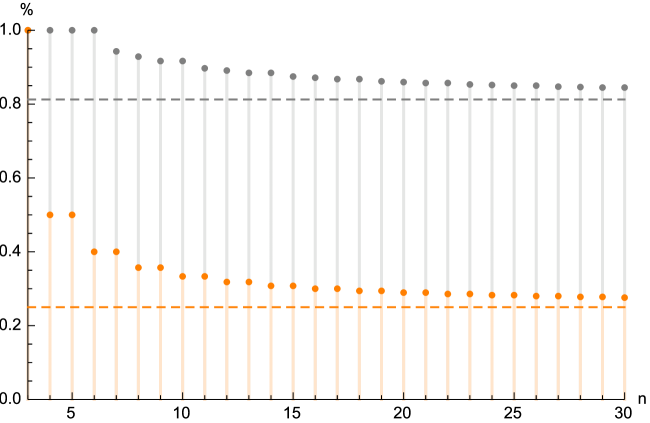Let us consider the first few values of $\mathcal{I}(n)/\binom{n}{3}$ and $\mathcal{Y}(n)/\binom{n}{3}$ (Fig. 11).

We can see that for small graphs the percentage of inconsistent triads is higher than for the larger graphs. In particular, for $n=3,\ldots,6$ there are such gt-graphs that have all triads inconsistent. However, there is only one t-graph which has all triads inconsistent. It is just a single triad. Although the percentage of inconsistent triads for both t-graph and gt-graph decrease, they seem to never drop below certain values. It is easy to compute that⁶⁶6Expression $\lim_{n\rightarrow\infty}\mathcal{I}(n)/\binom{n}{3}=0.25$ means that both $\lim_{n\rightarrow\infty}\left(\frac{n^{3}-n}{24}\right)/\binom{n}{3}=\lim_{n\rightarrow\infty}\left(\frac{n^{3}-4n}{24}\right)/\binom{n}{3}=0.25$ . Similarly $\lim_{n\rightarrow\infty}\frac{\mathcal{Y}(n)}{\binom{n}{3}}=0.8125$ means that all four limits (see 79) equal $0.8125$ . :

\lim_{n\rightarrow\infty}\frac{\mathcal{I}(n)}{\binom{n}{3}}=0.25\,\,\,\,\,\text{and}\,\,\,\,\,\lim_{n\rightarrow\infty}\frac{\mathcal{Y}(n)}{\binom{n}{3}}=0.8125

(82)

In other words, although in the larger t-graphs $(n>3)$ and gt-graphs $(n>6)$ , there must always be consistent triads. Hence, it is impossible to create a completely inconsistent set of paired comparisons when the alternatives are more than $3$ (without ties) and $6$ (when ties are allowed). As we can see very often, consistent triads must exist. However, it should be remembered that the “guaranteed” number of consistent triads is limited. The expression (82) implies that at most $75\%$ of triads are “guaranteed” to be consistent without ties, and at most $18.75\%$ of triads are “guaranteed” to be consistent when ties are allowed.

Figuratively speaking, the possibility of a tie allows us to be much more inconsistent. However, we rarely have a chance to be completely inconsistent - only when there are “sufficiently few” alternatives. Fortunately, there is no limit to the number of consistent triads in a gt-graph. Hence, we can be as consistent (and as frequently) in our views as we want.

7 Discussion and remarks

To calculate the inconsistency index $\zeta$ or the generalized inconsistency index $\zeta_{g}$ for some ordinal PC $M$ $n\times n$ matrix we need to determine the number of inconsistent triads in $M$ . The most straightforward method is to consider every single triad and decide whether it is consistent or not. Since in every complete set of paired comparisons for $n$ alternatives there are $\binom{n}{3}=\frac{n(n-1)(n-2)}{3}$ different triads, then the running time of such a procedure is $O(n^{3})$ . For t-graphs, however, there is a faster way to determine the number of inconsistent triads in a graph. As mentioned earlier, (5) denotes the number of inconsistent triads $\left|T\right|_{i}$ in some t-graph $T=(V,E_{d})$ . To compute (5) $\left|T\right|_{i}$ we need to visit every vertex $c\in V$ and determine its input degree. Computing $\text{deg}_{in}(c)$ for every $c\in V$ requires visiting every edge $(c_{i},c_{j})\in E_{d}$ twice. The first time when calculating $\text{deg}_{in}(c_{i})$ , the second time when $\text{deg}_{in}(c_{j})$ is calculated. Thus, determining $\text{deg}_{in}(c_{1}),\ldots,\text{deg}_{in}(c_{n})$ requires $2\left|E_{d}\right|$ operations. As $\left|E_{d}\right|=\frac{n(n-1)}{2}$ then the actual running time of computation for (5) is $O(n(n-1))=O(n^{2})$ . For this reason the inconsistency index $\zeta$ can be determined faster than $\zeta_{g}$ .

Looking at the different types of triads occurring in a gt-graph (Fig. 4), one may notice that a triad not covered by any directed edge is consistent, whilst a triad covered by one directed edge is always inconsistent (see Def. 7). Therefore the question arises as to whether it is possible to cover all triads by one directed edge. If not, what is the minimal number of directed edges covering all triads? Let us try to formally address this question. Denote the set of directed edges of some gt-graph by $E_{d}=\{(c_{1},c_{2}),(c_{1},c_{3}),\ldots,(c_{n-1},c_{n})\}$ and the set of triads by $\mathcal{T}=\{\{c_{1},c_{2},c_{3}\},\{c_{1},c_{2},c_{4}\},\ldots,\{c_{n-2},c_{n-1},c_{n}\}\}$ . Of course, $\left|E_{d}\right|=\binom{n}{2}$ and $\left|\mathcal{T}\right|=\binom{n}{3}$ . Then, let $B=(V,E)$ be a bipartite graph such that $V=E_{d}\cup\mathcal{T}$ and $E=\{(e,t)\,\,|\,\,(e,t)\in E_{d}\times\mathcal{T}\,\,\text{and}\,\,e\,\,\text{covers}\,\,t\}$ . Hence, we would like to select the minimal subset of edges from $E_{d}$ whose elements cover (i.e. are connected to) every triad in $\mathcal{T}$ .

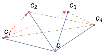
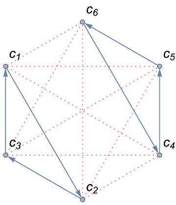
Let us consider the problem for $n=5$ (Fig. 12a).

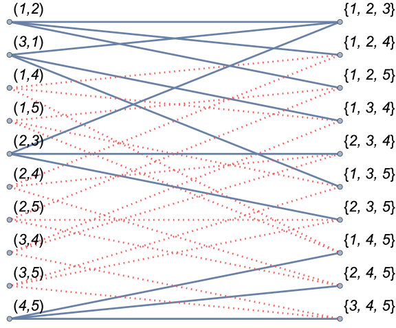
In such a case $E_{d}=\{(1,2)$ , $(1,3)$ , $(1,4)$ , $(1,5)$ , $(2,3)$ , $(2,4)$ , $(2,5)$ , $(3,4)$ , $(3,5)$ , $(4,5)\}$ and $\mathcal{T}=\{\{1,2,3\}$ , $\{1,2,4\}$ , $\{1,2,5\}$ , $\{1,3,4\}$ , $\{1,3,5\}$ , $\{2,3,4\}$ , $\{2,3,5\}$ , $\{1,4,5\}$ , $\{2,4,5\}$ , $\{3,4,5\}\}$ . As every edge covers three different triads we may form the set $S=\{\{t_{i},t_{j},t_{k}\}\,|$ $\,t,t_{j},t_{k}\in\mathcal{T},$ $\exists e\in E_{d}\,\text{that covers}\,\,t_{i},t_{j},t_{k}\}$ . For example, a tripleton $\{\{1,2,3\},\{1,2,4\},\{1,2,5\}\}$ is an element of $S$ as all its elements are covered by edges $(1,2)$ etc. Thus, the question about the minimal subset of $\left|E_{d}\right|$ whose elements cover all the elements in $\left|\mathcal{T}\right|$ , can be reformulated as follows: what is the minimal subset of $S$ such that the union of its elements equals $\mathcal{T}$ ?

In general, we can not provide a satisfactory answer to such a question. The problem we formulate is called a set cover problem⁷⁷7Wikipedia may serve as a quick reference: https://en.wikipedia.org/wiki/Set_cover_problem and is one of Karp’s 21 NP-complete problems formulated in 1972 [24]. Fortunately, we are not dealing with a set cover problem as such, but with its special instance that can be called a “triads cover problem”. In the latter case, a maximal dt-graph comes to the rescue (1). The number of directed edges in the maximal dt-graph is $\mathcal{X}(n)$ . Due to (Lemma 7) we know that every gt-graph that has less than $\mathcal{X}(n)$ directed edges must contain at least one triad of the type $\textit{CT}_{0}$ . On the other hand, any maximal dt-graph does not contain uncovered triads (Lemma 6). This means that a maximal dt-graph is a minimal graph covering all triads by directed edges.

Let us consider the maximal dt-graph for $n=5$ . According to (Proposition 1), such a graph should be composed of two maximal subgraphs having $\left\lfloor\frac{5}{2}\right\rfloor=3$ and $\left\lceil\frac{5}{2}\right\rceil=2$ vertices. An instance of the first subgraph can be a triad $(c_{1},c_{2}),\,(c_{2},c_{3})$ and $(c_{3},c_{1})$ whilst the second subgraph is just a single edge $(c_{4},c_{5})$ . As the maximal dt-graph with $5$ vertices provides a minimal edge covering of triads in $5$ -clique then the minimal subset of $S$ that covers the entire $\mathcal{T}$ is, for example, $\{\{1,2,3\}$ , $\{1,2,4\}$ , $\{1,2,5\}\}$ , $\{\{1,2,3\}$ , $\{1,3,4\}$ , $\{1,3,5\}\}$ $\{\{1,2,3\}$ , $\{2,3,4\}$ , $\{2,3,5\}\}$ and $\{\{1,4,4\}$ , $\{2,4,5\}$ , $\{3,4,5\}\}$ (Fig. 12).

8 Summary

In the presented article, the inconsistency index proposed by Kendall and Babington Smith [26] has been extended to cover pairwise comparisons with ties. For this purpose, the most inconsistent sets of pairwise comparisons with and without ties have been analyzed. To model pairwise comparisons with ties a generalized tournament graph has been defined. An additional absolute consistency index $\eta$ for pairwise comparisons with and without ties has also been proposed. The relationship between the maximally inconsistent set of pairwise comparisons with ties and the set cover problem has also been shown.

Acknowledgements

I would like to thank Prof. Andrzej Bielecki and Dr. Hab. Adam Sędziwy for their insightful comments, corrections and reading of the first version of this work. Special thanks are due to Ian Corkill for his editorial help. The research is supported by AGH University of Science and Technology, contract no.: 11.11.120.859.

Literature

References

[1] J. Aguarón and J. M. Moreno-Jiménez. The geometric consistency index: Approximated thresholds. European Journal of Operational Research, 147(1):137 – 145, 2003.
[2] S. Bozóki, L. Dezső, A. Poesz, and J. Temesi. Analysis of pairwise comparison matrices: an empirical research. Annals of Operations Research, 211(1):511–528, February 2013.
[3] S. Bozóki, J. Fülöp, and W. W. Koczkodaj. An lp-based inconsistency monitoring of pairwise comparison matrices. Mathematical and Computer Modelling, 54(1-2):789–793, 2011.
[4] M. Brunelli. On the conjoint estimation of inconsistency and intransitivity of pairwise comparisons. Operations Research Letters, 44(5):672–675, September 2016.
[5] M. Brunelli, L. Canal, and M. Fedrizzi. Inconsistency indices for pairwise comparison matrices: a numerical study. Annals of Operations Research, 211:493–509, February 2013.
[6] J. M. Colomer. Ramon Llull: from ‘Ars electionis’ to social choice theory. Social Choice and Welfare, 40(2):317–328, October 2011.
[7] M. Condorcet. Essay on the Application of Analysis to the Probability of Majority Decisions. Paris: Imprimerie Royale, 1785.
[8] A. H. Copeland. A “reasonable” social welfare function. Seminar on applications of mathematics to social sciences, 1951.
[9] H. A. David. The method of paired comparisons. A Charles Griffin Book, 1969.
[10] R. R. Davidson. On extending the Bradley-Terry model to accommodate ties in paired comparison experiments. Journal of the American Statistical Association, 65(329):317, 1970.
[11] Reinhard Diestel. Graph theory. Springer Verlag, 2005.
[12] P. Faliszewski, E. Hemaspaandra, L. A. Hemaspaandra, and J. Rothe. Llull and Copeland Voting Computationally Resist Bribery and Constructive Control. J. Artif. Intell. Res. (JAIR), 35:275–341, 2009.
[13] M Fedrizzi and M Brunelli. On the priority vector associated with a reciprocal relation and a pairwise comparison matrix. Journal of Soft Computing, 14(6):639–645, 2010.
[14] J. Figueira, M. Ehrgott, and S. Greco, editors. Multiple Criteria Decision Analysis: State of the Art Surveys. Springer, 2005.
[15] W A Glenn and H A David. Ties in paired-comparison experiments using a modified Thurstone-Mosteller model. Biometrics, 16(1):86, 1960.
[16] R. L. Graham, D. E Knuth, and O. Patashnik. Concrete Mathematics. Addison & Wesley, 1994.
[17] S. Greco, B. Matarazzo, and R. Słowiński. Dominance-based rough set approach to preference learning from pairwise comparisons in case of decision under uncertainty. In Eyke Hüllermeier, Rudolf Kruse, and Frank Hoffmann, editors, Computational Intelligence for Knowledge-Based Systems Design, volume 6178 of Lecture Notes in Computer Science, pages 584–594. Springer Berlin Heidelberg, 2010.
[18] Y. Iida. Ordinality consistency test about items and notation of a pairwise comparison matrix in AHP. In Proceedings of the international symposium on the …, 2009.
[19] A. Ishizaka and M. Lusti. How to derive priorities in AHP: a comparative study. Central European Journal of Operations Research, 14(4):387–400, December 2006.
[20] R. Janicki and W. W. Koczkodaj. A weak order approach to group ranking. Comput. Math. Appl., 32(2):51–59, July 1996.
[21] R. Janicki and Y. Zhai. On a pairwise comparison-based consistent non-numerical ranking. Logic Journal of the IGPL, 20(4):667–676, 2012.
[22] R. E. Jensen and T. E. Hicks. Ordinal data AHP analysis: A proposed coefficient of consistency and a nonparametric test. Math. Comput. Model., 17(4-5):135–150, February 1993.
[23] J. B. Kadane. Some Equivalence Classes in Paired Comparisons. The Annals of Mathematical Statistics, 37(2):488–494, April 1966.
[24] R. M. Karp. Reducibility among Combinatorial Problems. In Complexity of Computer Computations, pages 85–103. Springer US, Boston, MA, 1972.
[25] M. G. Kendall. The treatment of ties in ranking problems. Biometrika, 33:239–251, November 1945.
[26] M.G. Kendall and B. Smith. On the method of paired comparisons. Biometrika, 31(3/4):324–345, 1940.
[27] W. W. Koczkodaj. A new definition of consistency of pairwise comparisons. Math. Comput. Model., 18(7):79–84, October 1993.
[28] K. Kułakowski. On the properties of the priority deriving procedure in the pairwise comparisons method. Fundamenta Informaticae, 139(4):403 – 419, July 2015.
[29] K. Kułakowski, K. Grobler-Dębska, and J. Wąs. Heuristic rating estimation: geometric approach. Journal of Global Optimization, 62(3):529–543, 2015.
[30] A. Maas, T. Bezembinder, and P. Wakker. On solving intransitivities in repeated pairwise choices. Mathematical Social Sciences, 29(2):83–101, April 1995.
[31] E. Parizet. Paired comparison listening tests and circular error rates. Acta acustica united with Acustica, 2002.
[32] J.I. Peláez and M.T. Lamata. A new measure of consistency for positive reciprocal matrices. Computers & Mathematics with Applications, 46(12):1839 – 1845, 2003.
[33] S. Pemmaraju and S. Skiena. Computational Discrete Mathematics - Combinatorics and Graph Theory with Mathematica. Cambridge University Press, January 2003.
[34] T. L. Saaty. A scaling method for priorities in hierarchical structures. Journal of Mathematical Psychology, 15(3):234 – 281, 1977.
[35] T. L. Saaty and G. Hu. Ranking by eigenvector versus other methods in the analytic hierarchy process. Applied Mathematics Letters, 11(4):121–125, 1998.
[36] S. Siraj, L. Mikhailov, and J. A. Keane. Contribution of individual judgments toward inconsistency in pairwise comparisons. European Journal of Operational Research, 242(2):557–567, April 2015.
[37] W. E. Stein and P. J. Mizzi. The harmonic consistency index for the Analytic Hierarchy Process. European Journal of Operational Research, 177(1):488–497, February 2007.
[38] K. Suzumura, K. J. Arrow, and A. K. Sen. Handbook of Social Choice & Welfare. Elsevier Science Inc., 2010.
[39] L. L. Thurstone. The Method of Paired Comparisons for Social Values. Journal of Abnormal and Social Psychology, pages 384–400, 1927.
[40] T. N. Tideman. Independence of clones as a criterion for voting rules. Social Choice and Welfare, 4:185–206, 1987.
[41] L. G. Vargas. Voting with Intensity of preferences. In 12th International Symposium on the Analytic Hierarchy Process, Kuala Lumpur, Malaysia, 2013. Creative Decision Foundation.
[42] Ying-Ming Wang, C. Parkan, and Y. Luo. Priority estimation in the AHP through maximization of correlation coefficient. Applied Mathematical Modelling, 31(12):2711–2718, December 2007.

Appendix A Proof of Lemma 7

Thesis.

For every $n\in\mathbb{N}_{+},n\geq 3$ and $k\in\mathbb{N}_{+}$ it holds that:

\mathcal{F}(n,\mathcal{X}(n))=0

\mathcal{F}(n,\mathcal{X}(n)-k)\geq 1,\,\,\,\text{where}\,\,\,0<k\leq\mathcal{X}(n)

\mathcal{F}(n,\mathcal{X}(n)+k)\leq 0,\,\,\,\textit{where}\,\,\,0<k\leq\binom{n}{2}-\mathcal{X}(n)

Proof. Equation (65), part 1.

Let $n$ be even i.e. $n=2q$ where $q\in\mathbb{N}_{+}$ . Thus, let us insert to (49) as $n$ the value $2q$ and as $m$ the value $\mathcal{X}(2q)$ . After a series of elementary transformations applied to (48) we obtain:

\displaystyle\mathcal{F}(2q,\mathcal{X}(2q))

\displaystyle=\frac{1}{3}(-2)q\left(\lfloor q\rfloor^{2}+(1-2q)\lfloor q\rfloor+(q-1)q\right)

(82)

Since $q\in\mathbb{N}_{+}$ then

\lfloor q\rfloor=q

(83)

Thus,

\displaystyle\mathcal{F}(2q,\mathcal{X}(2q))

\displaystyle=\frac{1}{3}(-2)q\left(q^{2}+(q-1)q+(1-2q)q\right)

(84)

Which after reduction leads to

\mathcal{F}(2q,\mathcal{X}(2q))=0

(85)

Proof. Equation (65), part 2.

Let $n$ be odd i.e. $n=2q+1$ where $q\in\mathbb{N}_{+}$ . Similarly, let us replace n in (49) by $2q+1$ and $m$ by $\mathcal{X}(2q+1)$ . After elementary transformations we obtain:

$\displaystyle\mathcal{F}(2q+1,\mathcal{X}(2q+1))=$	$\displaystyle-\frac{1}{3}(2q+1)\left\lfloor\frac{2q^{2}}{2q+1}\right\rfloor^{2}$
	$\displaystyle+\frac{1}{3}\left(4q^{2}-2q-1\right)\left\lfloor\frac{2q^{2}}{2q+1}\right\rfloor$
	$\displaystyle+\frac{1}{3}\left(-2q^{2}+3q-1\right)q$	(86)

Since $q\in\mathbb{N}_{+}$ , we can bound $2q^{2}/\left(2q+1\right)$ from above

\frac{2q^{2}}{2q+1}<\frac{2q^{2}}{2q}=q

(87)

and below

q-1=\frac{2\left(q-1\right)^{2}}{2\left(q-1\right)}<\frac{2\left(q-1\right)^{2}}{2q+1}=\frac{2q^{2}-2q+2}{2q+1}\leq\frac{2q^{2}}{2q+1}

(88)

Therefore, when $q$ is a positive integer it is true that

\left\lfloor\frac{2q^{2}}{2q+1}\right\rfloor=(q-1)

(89)

By applying (89) to (86) we obtain

$\displaystyle\mathcal{F}(2q+1,\mathcal{X}(2q+1))$	$\displaystyle=\frac{1}{3}\left(4q^{2}-2q-1\right)(q-1)$
	$\displaystyle+\frac{1}{3}q\left(-2q^{2}+3q-1\right)$
	$\displaystyle-\frac{1}{3}(2q+1)\left(q-1\right)^{2}$	(90)

Then, after making further transformations it is easy to verify that:

\mathcal{F}(2q+1,\mathcal{X}(2q+1))=0

(91)

which completes the proof of (65).

Proof. Equation (66), part 1.

Let $n$ be even i.e. $n=2q$ where $q\in\mathbb{N}_{+}$ . Thus, to prove that $\mathcal{F}(n,\mathcal{X}(n)-k)$ is greater than $0$ it is enough to show that for every $q\geq 2$ and $1\leq k<q(q-1)$ it holds that $\mathcal{F}(n,\mathcal{X}(n)-k)>1$ . Thus, let us insert to (49) as $n$ the value $2q$ . After a series of elementary transformations applied to (48) we obtain:

\mathcal{F}(2q,\mathcal{X}(2q)-k)=\frac{2}{3}\left(-q\left\lceil\frac{k}{q}\right\rceil^{2}+(2k+q)\left\lceil\frac{k}{q}\right\rceil+k(q-1)\right)

(92)

Let us observe that for the positive integer $p=1,2,\ldots$ if $p\cdot q\leq k<(p+1)q-1$ then $\left\lceil\frac{k}{q}\right\rceil=p$ . In order to analyze $\mathcal{F}$ let us replace $\left\lceil\frac{k}{q}\right\rceil$ by $p$ and define $h$ such that

h(q,k)=\frac{2}{3}\left(p(2k+q)+k(q-1)-qp^{2}\right)

(93)

where $p\cdot q\leq k<(p+1)q-1$ for every $p=1,2,\ldots,q-2$ . Of course, when $p\cdot q\leq k<(p+1)q-1$ it holds that

\mathcal{F}(2q,\mathcal{X}(2q)-k)=h(q,k)

(94)

As $h$ is linear with respect to $k$ then in order to check whether $h(k)>0$ it is enough to check whether $h$ is greater than $0$ at both ends of the considered interval. So,

h(q,p\cdot q)=\frac{2}{3}pq(p+q)

(95)

and

h(q,(p+1)q-1)=\frac{1}{3}\left(2p^{2}q+2pq^{2}+4pq-4p+2q^{2}-4q+2\right)

(96)

Since for $p,q=1,2,\ldots$ it holds that $4pq\geq 4p$ and $2p^{2}q+2pq^{2}\geq 4q$ then

h(q,(p+1)q-1)\geq\frac{1}{3}\left(2q^{2}+2\right)\geq\frac{1}{3}\left(2+2\right)>1

(97)

Thus, for every $p\cdot q\leq k<(p+1)q-1$ where $p=1,2,\ldots,q-2$ , $h(k)>0$ . We just need to check $h$ for $k=q(q-1)$ . In such a case $\left\lceil\frac{k}{q}\right\rceil=q-1$ . Thus $h(q(q-1))$ takes the form:

h(q,q(q-1))=\frac{2}{3}q\left(2q^{2}-3q+1\right)

(98)

As $q\geq 2$ then it is easy to verify that $h(q,q(q-1))>0$ .

Since $h(q,k)>0$ for every $p=1,2,\ldots,q-2$ , where $p\cdot q\leq k<(p+1)q-1$ and for $k=q(q-1)$ then also $\mathcal{F}(2q,\mathcal{X}(2q)-k)>0$ for $n=2q$ and $1\leq k<q(q-1)$ , which completes the first part of the proof.

Proof. Equation (66), part 2.

Let $n$ be even i.e. $n=2q+1$ where $q\in\mathbb{N}_{+}$ . Thus, let us insert to (49) as $n$ the value $2q+1$ and $\mathcal{X}(2q+1)-k$ , where this time $1\leq k\leq q^{2}$ (see 63). After a series of elementary transformations applied to (48) we obtain:

	$\displaystyle\mathcal{F}(n,\mathcal{X}(n)-k)=$	$\displaystyle\frac{1}{3}\left((4k+2q+1)\left\lceil\frac{2\left(k-q^{2}\right)}{2q+1}\right\rceil+4q^{2}\left\lfloor\frac{2\left(q^{2}-k\right)}{2q+1}\right\rfloor-\right.$
		$\displaystyle\left.(2q+1)\left\lfloor\frac{2\left(q^{2}-k\right)}{2q+1}\right\rfloor^{2}+(2q-1)\left(3k-q^{2}+q\right)\right)$		(99)

Since for every $x\in\mathbb{R}$ it holds ⁸⁸8A quick reference is https://en.wikipedia.org/wiki/Floor_and_ceiling_functions [16] that $-\left\lceil x\right\rceil=\left\lfloor-x\right\rfloor$ , and $\mathcal{X}(n)=\mathcal{X}(2q+1)=q^{2}$ then

	$\displaystyle\mathcal{F}(2q+1,q^{2}-k)=$	$\displaystyle\frac{1}{3}\left(-(4k+2q+1)\left\lfloor\frac{2\left(q^{2}-k\right)}{2q+1}\right\rfloor+4q^{2}\left\lfloor\frac{2\left(q^{2}-k\right)}{2q+1}\right\rfloor-\right.$
		$\displaystyle\left.(2q+1)\left\lfloor\frac{2\left(q^{2}-k\right)}{2q+1}\right\rfloor^{2}+(2q-1)\left(3k-q^{2}+q\right)\right)$		(100)

It is easy to observe the relationship between $\left\lfloor\frac{2\left(q^{2}-k\right)}{2q+1}\right\rfloor$ and $k$ is:

$\left\lfloor\frac{2\left(q^{2}-k\right)}{2q+1}\right\rfloor=0$ if and only if $0\leq 2\left(q^{2}-k\right)<2q+1$ , in other words, we require that $q^{2}-q-\frac{1}{2}\leq k<q^{2}$

$\left\lfloor\frac{2\left(q^{2}-k\right)}{2q+1}\right\rfloor=1$ if and only if $2q+1\leq 2\left(q^{2}-k\right)<2(2q+1)$ which translates to the interval: $\frac{1}{2}\left(2q^{2}-2\left(2q+1\right)\right)\leq k<\frac{1}{2}\left(2q^{2}-1\left(2q+1\right)\right)$

$\left\lfloor\frac{2\left(q^{2}-k\right)}{2q+1}\right\rfloor=2$ if and only if $2(2q+1)\leq 2\left(q^{2}-k\right)<3(2q+1)$ , hence $\frac{1}{2}\left(2q^{2}-3\left(2q+1\right)\right)\leq k<\frac{1}{2}\left(2q^{2}-2\left(2q+1\right)\right)$

and in general, $r\overset{\textit{df}}{=}\left\lfloor\frac{2\left(q^{2}-k\right)}{2q+1}\right\rfloor$ if and only if $(r-1)(2q+1)\leq 2\left(q^{2}-k\right)<r(2q+1)$ , which translates to the interval for $k$ : $\frac{1}{2}\left(2q^{2}-r\left(2q+1\right)\right)\leq k<\frac{1}{2}\left(2q^{2}-(r-1)\left(2q+1\right)\right)$ .

Thus, instead of analyzing $\mathcal{F}$ with respect to $k$ over the whole domain i.e. $1\leq k\leq q^{2}$ and $q\geq 2$ we can analyze it in the subsequent intervals, in which the value $\left\lfloor\frac{2\left(q^{2}-k\right)}{2q+1}\right\rfloor$ is known and fixed.

Let us introduce the auxiliary function $h:$

h(q,k,r)\overset{\textit{df}}{=}\mathcal{F}(2q+1,q^{2}-k)

(101)

defined for $k$ such that $\frac{1}{2}\left(2q^{2}-r\left(2q+1\right)\right)\leq k<\frac{1}{2}\left(2q^{2}-(r-1)\left(2q+1\right)\right)$ . Hence,

h(q,k,r)=\frac{1}{3}\left(-(4k+2q+1)r+4q^{2}r-(2q+1)r^{2}+(2q-1)\left(3k-q^{2}+q\right)\right)

(102)

Moreover, $r$ is the highest when $k$ is $1$ . Thus, due to (89) it holds that $\left\lfloor\frac{2\left(q^{2}-1\right)}{2q+1}\right\rfloor\leq\left\lfloor\frac{2q^{2}}{2q+1}\right\rfloor=q-1$ . Therefore, we know that $r\leq q-1$ . Hence, instead of showing that $\mathcal{F}(2q+1,q^{2}-k)>1$ for every $0\leq k\leq q^{2}$ , we prove that $h(q,k,r)>1$ when $\frac{1}{2}\left(2q^{2}-r\left(2q+1\right)\right)\leq k<\frac{1}{2}\left(2q^{2}-(r-1)\left(2q+1\right)\right)$ for every $0\leq r\leq q-1$ .

Let us observe that $h(q,k,r)$ is a decreasing function with respect to $k$ . That is because

h(q,k,r)-h(q,k-1,r)=2q-\frac{4r}{3}+1

(103)

where $r\leq q-1$ . In particular, it is easy to verify that always $2q+1>\frac{4r}{3}$ for $r\leq q-1$ .

The above equalities justify the following estimation:

h(q,k,r)>h(q,k-1,r)>\ldots>h(q,\frac{1}{2}\left(2q^{2}-r\left(2q+1\right)\right),r)

(104)

Thus, to prove that $h(q,k,r)>0$ for all admissible values of $q,k,r$ we need to check whether $h(q,\frac{1}{2}\left(2q^{2}-r\left(2q+1\right)\right),r)>0$ for $0\leq r\leq q-1$ .

So, applying the lower bound for $k$ , i.e. $k=\frac{1}{2}\left(2q^{2}-r\left(2q+1\right)\right)$ to (102) we obtain

h(q,\frac{1}{2}\left(2q^{2}-r\left(2q+1\right)\right),r)=\frac{1}{6}(2q+1)\left(4q^{2}-6qr-2q+2r^{2}+r\right)

(105)

Let us denote $h_{2}(q,r)\overset{\textit{df}}{=}h(q,\frac{1}{2}\left(2q^{2}-r\left(2q+1\right)\right),r)$ . It is easy to observe that $h_{2}$ is a parabola with respect to $r$ . Since $\frac{\partial^{2}h_{2}}{\partial r^{2}}=\frac{2}{3}(2q+1)$ is greater than $0$ for $q\geq 2$ , thus $h_{2}(q,r)$ has the minimum with respect to $r$ when $\frac{\partial h_{2}}{\partial r}=0$ . I.e.

\frac{\partial h_{2}}{\partial r}=-\frac{1}{6}(2q+1)(6q-4r-1)=0

(106)

i.e., when

r=\frac{1}{4}(6q-1)

(107)

In other words, $h_{2}$ decreases for $r=1,2,\ldots$ , then reaches the minimum⁹⁹9In fact, due to the diophantic nature of $h_{2}$ , its minimum is either at $\left\lfloor\frac{1}{4}(6q-1)\right\rfloor$ or $\left\lceil\frac{1}{4}(6q-1)\right\rceil$ . at $r=\frac{1}{4}(6q-1)$ , next starts to increase for $r\geq\left\lceil\frac{1}{4}(6q-1)\right\rceil$ . However, $h,h_{2}$ are defined for $r\leq q-1$ . Thus, it is clear that within the interval $0\leq r\leq q-1$ the function $h_{2}$ is strictly decreasing with respect to $r$ . Moreover, it is easy to verify that $q-1<\left\lfloor\frac{1}{4}(6q-1)\right\rfloor$ . Thus, to determine the minimal value of $h_{2}$ it is enough to check their value for $r=q-1$ .

Thus $h_{2}$ :

h_{2}(q,q-1)=\frac{1}{6}\left(2q^{2}+3q+1\right)

(108)

Since, $q\geq 2$ then it is easy to verify that $h_{2}(q,q-1)>0$ . This implies that $h(q,k,r)>0$ for every $0\leq r\leq q-1$ and $k$ such that $\frac{1}{2}\left(2q^{2}-r\left(2q+1\right)\right)\leq k<\frac{1}{2}\left(2q^{2}-(r-1)\left(2q+1\right)\right)$ . Hence, also $\mathcal{F}(n,\mathcal{X}(n)-k)>0$ for $n=2q+1$ where $1\leq k\leq q^{2}$ , which completes the proof of (66).

Proof. Equation (67), part 1.

Let $n$ be even i.e. $n=2q$ where $q\in\mathbb{N}_{+}$ . Since (4) to prove that $\mathcal{F}(n,\mathcal{X}(n)+k)$ is smaller than $0$ it is enough to show that for every integer $q,k$ such that $q\geq 2$ and $1\leq k\leq\binom{n}{2}-\mathcal{X}(n)$ where $\binom{n}{2}-\mathcal{X}(n)=\binom{2q}{2}-q(q-1)=q^{2}$ it holds that $\mathcal{F}(2q,q(q-1)+k)\leq 0$ . After a series of elementary transformations applied to (48) we obtain that:

\mathcal{F}(2q,q(q-1)+k)=-\frac{2}{3}\left(q\left\lfloor\frac{k}{q}\right\rfloor^{2}+(q-2k)\left\lfloor\frac{k}{q}\right\rfloor+k(q-1)\right)

(109)

Let us consider the relationship between $k$ and $\left\lfloor\frac{k}{q}\right\rfloor$ . When $1\leq k<q$ it holds that $\left\lfloor\frac{k}{q}\right\rfloor=0$ , when $q\leq k<2q$ it holds that $\left\lfloor\frac{k}{q}\right\rfloor=1$ and similarly, $2q\leq k<3q$ then it holds that $\left\lfloor\frac{k}{q}\right\rfloor=2$ . In general, when $rq\leq k<(r+1)q$ then $\left\lfloor\frac{k}{q}\right\rfloor=r$ . Of course, since $k\leq q^{2}$ then $r\leq q$ . Hence, instead of considering the function $\mathcal{F}$ at once, we may analyze it in the intervals in which $\left\lfloor\frac{k}{q}\right\rfloor$ is known and constant. Let us define:

f(q,k,r)\overset{\textit{df}}{=}qr^{2}+(q-2k)r+k(q-1)

(110)

It is easy to see that $f(q,k,r)=-\frac{3}{2}\cdot\mathcal{F}(2q,q(q-1)+k)$ if $rq\leq k<(r+1)q$ for $r=0,\ldots,q-1$ . Hence, instead of analyzing $\mathcal{F}$ we will focus on the auxiliary function $f.$

The first observation is that $f$ is linear with respect to $k$ providing that $q$ and $r$ are known and fixed. Thus, the minimal value of $f$ with respect to $k$ within the interval $rq\leq k<(r+1)q$ is $\min\{f(q,rq,r),f(q,(r+1)q,r)\}$ . In other words, it is enough to check that $f$ is greater than $0$ at both edges of the interval for $k$ . Let us consider $f$ at the lower bound, i.e. for $k=rq$ .

f(q,rq,r)=qr(q-r)

(111)

It is easy to verify that for every $0<r<q$ and $q\geq 2$ the value $f(q,rq,r)>0$ . The function $f(q,rq,r)$ reaches $0$ when $r=0$ . Thus, $f(q,rq,r)\geq 0$ for every $r$ such that $0\leq r\leq q$ .

Let us consider $f$ at the other end of interval, i.e. for $k=(r+1)q-1$ .

f(q,(r+1)q-1,r)=q^{2}(r+1)-q\left(r^{2}+2r+2\right)+2r+1

(112)

Similarly as above, we would like to show that for every admissible $r$ the function $f(q,(r+1)q-1,r)\geq 0$ . Hence, let us rewrite $f$ with respect to $r$ .

f(q,(r+1)q-1,r)=-qr^{2}+r\left(q^{2}-2q+2\right)+\left(q^{2}-2q+1\right)

(113)

When considering $f$ as a polynomial with respect to $r$ one may notice that the coefficient at $r^{2}$ is negative ( $-q<0$ ) which means that $f$ is concave.

Let us denote $f_{2}(q,r)\stackrel{{\scriptstyle\textit{df}}}{{=}}f(q,(r+1)q-1,r)$ . It is easy to compute that $\frac{\partial f_{2}}{\partial r}=0$ when $r=\frac{q^{2}-2q+2}{2q}$ . Since $\frac{\partial^{2}f_{2}}{\partial r^{2}}=-2q>0$ , thus $f_{2}$ reaches the maximum¹⁰¹⁰10In fact, due to the diophantine nature of $f$ it reaches the maximum for $r=\left\lfloor\frac{q^{2}-2q+2}{2q}\right\rfloor$ or $r=\left\lceil\frac{q^{2}-2q+2}{2q}\right\rceil$ . for $r=\frac{q^{2}-2q+2}{2q}$ . Since the interval of $r$ is $0\leq r<q$ and also $0\leq\frac{q^{2}-2q+2}{2q}<q$ therefore the minimum of $f_{2}$ for $0\leq r<q$ is the smaller of the two $f_{2}(q,0)$ and $f_{2}(q,q-1)$ .

Hence

f_{2}(q,0)=q^{2}-2q+1,\,\,\,\,f_{2}(q,q-1)=q-1

(114)

Since for every $q\geq 2$ it holds that $\min\{f_{2}(q,0),f_{2}(q,q-1)\}\geq 0$ then $f_{2}(q,r)\geq 0$ for every fixed $q\geq 2$ and $0\leq r<q$ , which implies that also for $k=(r+1)q-1$ , $f(q,k,r)\geq 0$ . Therefore $f(q,k,r)\geq 0$ for every $rq\leq k<(r+1)q$ for $r=0,\ldots,q$ .

As $f(q,k,r)=-\frac{3}{2}\cdot\mathcal{F}(2q,q(q-1)+k)$ when $rq\leq k<(r+1)q$ , then due to the arbitrary choice of $r$ it holds that $\mathcal{F}(n,\mathcal{X}(n)+k)\leq 0$ for $n=2q$ and $0\leq k<q^{2}$ . As one may observe, the above reasoning does not cover $k=q^{2}$ . This is the last “point interval” that needs to be considered. For $k=q^{2}$ we have

\mathcal{F}(2q,q(q-1)+q^{2})=\frac{1}{3}(-2)q\left(\lfloor 2q\rfloor^{2}+(1-4q)\lfloor 2q\rfloor+2(2q-1)q\right)

(115)

Since $q\in\mathbb{N}_{+}$ then $\lfloor 2q\rfloor=2q$ . Hence it is easy to verify that

\mathcal{F}(2q,q(q-1)+q^{2})=0

(116)

Which completes the first part of the proof of (67).

Proof. Equation (67), part 2.

Let $n$ be odd i.e. $n=2q+1$ where $q\in\mathbb{N}_{+}$ . Since (4) to prove that $\mathcal{F}(n,\mathcal{X}(n)+k)$ is smaller than $0$ it is enough to show that for every integer $q,k$ such that $q\geq 2$ and $1\leq k\leq\binom{2q}{2}-q^{2}-1=q^{2}-q-1$ it holds that $\mathcal{F}(2q+1,q^{2}+k)\leq 0$ . After a series of elementary transformations applied to (48) we obtain:

$\displaystyle\mathcal{F}(2q+1,q^{2}+k)=$	$\displaystyle-\frac{1}{3}\left((2q+1)\left\lfloor\frac{2\left(q^{2}+k\right)}{2q+1}\right\rfloor^{2}\right.$
	$\displaystyle-\left(4k+4q^{2}-2q-1\right)\left\lfloor\frac{2\left(q^{2}+k\right)}{2q+1}\right\rfloor$	(117)
	$\displaystyle\left.\begin{array}[]{c}\\ \\ \\ \end{array}+(2q-1)(3k+(q-1)q)\right)$	(121)

Since $1\leq k\leq q^{2}-q-1$ we may estimate the upper and the lower bound for $\left\lfloor\frac{2\left(q^{2}+k\right)}{2q+1}\right\rfloor$ as

q-1\leq\left\lfloor\frac{2q^{2}}{2q+1}\right\rfloor+\left\lfloor\frac{2k}{2q+1}\right\rfloor\leq\left\lfloor\frac{2\left(q^{2}+k\right)}{2q+1}\right\rfloor

(122)

and

	$\displaystyle\left\lfloor\frac{2\left(q^{2}+k\right)}{2q+1}\right\rfloor\leq$	$\displaystyle\left\lfloor\frac{2\left(q^{2}+q^{2}-q-1\right)}{2q+1}\right\rfloor\leq\left\lfloor\frac{4q^{2}}{2q}-\frac{2q+2}{2q+1}\right\rfloor=$		(123)
		$\displaystyle\left\lfloor 2q-\frac{2q+2}{2q+1}\right\rfloor=\left\lfloor 2q-2\right\rfloor=2q-2$

Let us denote $r\overset{\textit{df}}{=}\left\lfloor\frac{2\left(q^{2}+k\right)}{2q+1}\right\rfloor$ . Thus, $q-1\leq r\leq 2q-2$ . Let us consider the relationship between $k$ and $r$ . It holds that $\left\lfloor\frac{2\left(q^{2}+k\right)}{2q+1}\right\rfloor=r$ wherever $r\leq\frac{2\left(q^{2}+k\right)}{2q+1}<r+1$ . Thus it is easy to determine that $\left\lfloor\frac{2\left(q^{2}+k\right)}{2q+1}\right\rfloor=r$ wherever $\frac{1}{2}\left(2qr+r-2q^{2}\right)\leq k<\frac{1}{2}\left(\left(r+1\right)\left(2q+1\right)-2q^{2}\right)$ .

Let us consider the function $\mathcal{F}(2q+1,q^{2}+k)$ for $k\in\mathbb{N}_{+}$ such that $\frac{1}{2}\left(2qr+r-2q^{2}\right)\leq k<\frac{1}{2}\left(\left(r+1\right)\left(2q+1\right)-2q^{2}\right)$ . For this purpose, let us define $f$

f(q,k,r)\overset{\textit{df}}{=}(2q+1)r^{2}-r\left(4k+4q^{2}-2q-1\right)+(2q-1)(3k+(q-1)q)

(124)

It is easy to verify that

\mathcal{F}(2q+1,q^{2}+k)=-\frac{1}{3}f(q,k,r)

(125)

providing that $q,r\in\mathbb{N}_{+}$ , $\frac{1}{2}\left(2qr+r-2q^{2}\right)\leq k<\frac{1}{2}\left(\left(r+1\right)\left(2q+1\right)-2q^{2}\right)$ , $q-1\leq r\leq 2q-2$ and $q\geq 2$ . Hence, wherever $f(q,k,r)\geq 0$ then $\mathcal{F}(2q+1,q^{2}+k)\leq 0$ . Let us observe that $f$ is linear with respect to $k$ . Therefore it is enough to check the value of $f(q,k,r)$ at the edges of the admissible interval for $k$ , and prove that those values are above $0$ in any possible interval determined by $r$ . For this purpose let us define

f_{2}(q,r)\stackrel{{\scriptstyle\textit{df}}}{{=}}f(q,\frac{1}{2}\left(2qr+r-2q^{2}\right),r)

(126)

for the lower bound, and

f_{3}(q,r)\stackrel{{\scriptstyle\textit{df}}}{{=}}f(q,\frac{1}{2}\left(\left(r+1\right)\left(2q+1\right)-2q^{2}\right)-1,r)

(127)

for the upper bound. Hence

f_{2}(q,r)=-\frac{1}{2}(2q+1)\left(4q^{2}-6qr-2q+2r^{2}+r\right)

(128)

f_{3}(q,r)=-4q^{3}+6q^{2}(r+1)-q\left(2r^{2}+2r+5\right)+\frac{1}{2}\left(-2r^{2}+3r+3\right)

(129)

Let us reorganize the above equations with respect to $r$ :

f_{2}(q,r)=-\left(2q+1\right)r^{2}+\left(2q+6q^{2}-\frac{1}{2}\right)r-4q^{3}+q

(130)

f_{3}(q,r)=-\left(2q+1\right)r^{2}+\left(6q^{2}-2q+\frac{3}{2}\right)r-4q^{3}+6q^{2}-5q+\frac{3}{2}

(131)

Since both $f_{2}$ and $f_{3}$ have second degree polynomials with respect to $r$ , and the coefficients nearby $r^{2}$ are negative, then $f_{2}$ and $f_{3}$ are concave parabolas. Therefore $f_{2}$ and $f_{3}$ are not smaller than $0$ within the interval $q-1\leq r\leq 2q-2$ if they are not negative at both ends of the interval i.e. $q-1$ and $2q-2$ . As the estimation (122) is not perfect, let us assume for a moment that $r$ is in $q\leq r\leq 2q-2$ , whilst the case $r=q-1$ we handle separately.

Let us examine (130).

f_{2}(q,r)=q^{2}+\frac{q}{2}\,\,\,\textit{when}\,\,\,\,r=q

(132)

and

f_{2}(q,r)=(2q-3)(2q+1)\,\,\,\textit{when}\,\,\,r=2q-2

(133)

Since $q\geq 2$ both of the above equations are greater than $0$ . For (131) it is enough to assume that $q-1\leq r\leq 2q-2$ . Thus,

f_{3}(q,r)=q^{2}-\frac{3q}{2}-1\,\,\,\textit{when}\,\,\,r=q-1

(134)

and

f_{3}(q,r)=2q^{2}+2q-\frac{11}{2}\,\,\,\textit{when}\,\,\,r=2q-2

(135)

Similarly, it is easy to verify that both of the above expressions are non negative as $q\geq 2$ .

At the end, let us explicitly calculate

f(q,k,q-1)=2kq+k

(136)

As $k$ is always non negative, then also in this case $f$ is non negative $0$ . Thereby for every $1\leq k\leq q^{2}-q-1$ it holds that $\mathcal{F}(2q+1,q^{2}+k)\leq 0$ which completes the proof of the Lemma 7 $\square$

Appendix B Proof of the Lemma 8

Thesis.

For every $n\in\mathbb{N}_{+},n\geq 3$ the function $\mathcal{C}$ :

1.

is constant and equals $\mathcal{C}(n,m)=0$ for every $m$ such that $0\leq m<n$
2.

is strictly increasing for every $m\in\mathbb{N}_{+}$ such that $n\leq m\leq\binom{n}{2}$ , i.e.

\mathcal{C}(n,m+1)-\mathcal{C}(n,m)>0

Proof. Claim 1.

The first claim that $\mathcal{C}(n,m)=0$ for every $m$ such that $0\leq m<n$ is a direct consequence of the equation (25). It is enough to note that the right side of expression (25) is the product where the first part is $\frac{1}{2}\left\lfloor\frac{m}{n}\right\rfloor$ . Hence, wherever $m<n$ the product often equals $0$ .

Proof. Claim 2.

Due to (Theorem 4) it holds that

	$\displaystyle\mathcal{C}(n,m+1)-\mathcal{C}(n,m)=$	$\displaystyle\frac{1}{2}\left(\left\lfloor\frac{m}{n}\right\rfloor\left(n\left\lfloor\frac{m}{n}\right\rfloor-2m+n\right)-\right.$
		$\displaystyle\left.\left\lfloor\frac{m+1}{n}\right\rfloor\left(n\left\lfloor\frac{m+1}{n}\right\rfloor-2m+n-2\right)\right)$		(136)

It is easy to observe that for some positive integer $p=1,2,\ldots$ when $m=np-1$ then $\left\lfloor\frac{m}{n}\right\rfloor=p-1,\left\lfloor\frac{m+1}{n}\right\rfloor=p$ . Next, by increasing $m$ by one we get $m=np$ and $\left\lfloor\frac{m}{n}\right\rfloor=p,\left\lfloor\frac{m+1}{n}\right\rfloor=p$ . Then, for $m=n(p+1)-1$ the values of our floored expressions change to $\left\lfloor\frac{m}{n}\right\rfloor=p,\left\lfloor\frac{m+1}{n}\right\rfloor=p+1$ , and then by increasing $m$ by one we get $\left\lfloor\frac{m}{n}\right\rfloor=p+1,\left\lfloor\frac{m+1}{n}\right\rfloor=p+1$ . Hence, there are two different intervals with respect to the values $\left\lfloor\frac{m}{n}\right\rfloor$ and $\left\lfloor\frac{m+1}{n}\right\rfloor$ . The first one in which both expressions have the same value, and the other one (composed of one point) in which their values differ by one. In general, we may observe that:

wherever $m=np-1$ then $\left\lfloor\frac{m}{n}\right\rfloor=p-1,\left\lfloor\frac{m+1}{n}\right\rfloor=p$ , and wherever $np\leq m<n(p+1)-1$ then $\left\lfloor\frac{m}{n}\right\rfloor=p,\left\lfloor\frac{m+1}{n}\right\rfloor=p$ .

Let us define the auxiliary function $h$ by replacing in (136) $\left\lfloor\frac{m}{n}\right\rfloor$ by $r$ and $\left\lfloor\frac{m+1}{n}\right\rfloor$ by $t$ :

h(n,m,r,t)\overset{\textit{df}}{=}\frac{1}{2}\left(r\left(nr-2m+n\right)-t\left(nt-2m+n-2\right)\right)

(137)

The function $h$ can be rewritten with respect to $m$ , so

h(n,m,r,t)=\frac{1}{2}nr^{2}+m\left(t-r\right)+\frac{1}{2}nr-\frac{1}{2}nt^{2}-\frac{1}{2}nt+t

(138)

It is easy to observe that

\mathcal{C}(n,m+1)-\mathcal{C}(n,m)=h(n,m,r,t)

(139)

where $r=\left\lfloor\frac{m}{n}\right\rfloor$ and $t=\left\lfloor\frac{m+1}{n}\right\rfloor$ . Thus, instead of analyzing $h(n,m,r,t)$ for $m$ such that $n\leq m\leq\binom{n}{2}$ we analyze $h(n,m,r,t)$ in two intervals $m=np-1$ and $np\leq m<n(p+1)-1$ . This, due to the arbitrary choice of $p$ , would apply to $\mathcal{C}(n,m+1)-\mathcal{C}(n,m)$ over the whole interval $n\leq m\leq\binom{n}{2}$ .

Let us observe that $h$ is linear with respect to $m$ . Thus to prove that $h(n,m,r,t)>0$ when $n,r,t$ are constant, one needs only to verify the value of $h$ at the ends of both intervals to which $m$ may belong. Thus, let us consider the first “point” interval $m=np-1$ . In this interval $\left\lfloor\frac{m}{n}\right\rfloor=p-1,\left\lfloor\frac{m+1}{n}\right\rfloor=p$ , thus:

h(n,np-1,p-1,p)=p-1

(140)

As $m\geq n$ , and $m=np-1$ thus $p\geq 2$ . Hence,

h(n,np-1,p-1,p)\geq 2-1=1

(141)

This supports the thesis of the theorem, i.e. $np\leq m<n(p+1)-1$ , where $\left\lfloor\frac{m}{n}\right\rfloor=p,\left\lfloor\frac{m+1}{n}\right\rfloor=p$ . For both its ends we have:

h(n,np,p,p)=p

(142)

h(n,n(p+1)-1,p,p)=p

(143)

As $m\geq n$ and $np\leq m$ then $p\geq 1$ . Thus in both cases $h$ is strictly greater than $0$ . Hence, for every $np-1\leq m\leq n(p+1)-1$ it holds that

\mathcal{C}(n,m+1)-\mathcal{C}(n,m)>0

(144)

Due to the arbitrary choice of $p$ this statement completes the proof of the theorem. $\square$

Appendix C Proof of the Lemma 9

Thesis.

For every $n\in\mathbb{N}_{+},n\geq 3$ it holds that

\binom{n}{3}-\mathcal{C}(n,\mathcal{X}(n))=\mathcal{Y}(n)

Proof. Part 1.

Let $n=4q$ ( $n$ is even, and $\left\lfloor\frac{n}{2}\right\rfloor=\left\lceil\frac{n}{2}\right\rceil=2q$ is even), $n\geq 4$ , hence $q\geq 1$ and $\mathcal{X}(4q)=2q(2q-1)$ . Thus to prove (69) for even numbers we show that

\binom{4q}{3}-\mathcal{C}(4q,2q(2q-1))-\mathcal{Y}(4q)=0

(144)

Since (64) reduces to:

	$\displaystyle\mathcal{Y}(4q)=$	$\displaystyle\binom{4q}{3}-\left(\binom{2q}{3}-\frac{q\left(q^{2}-1\right)}{3}\right)$
		$\displaystyle-\left(\binom{2q}{3}-\frac{q\left(q^{2}-1\right)}{3}\right)$		(145)

by elementary transformations one may show that (144) is equivalent to

2q\left(\left\lceil\frac{1}{2}-q\right\rceil+q-1\right)^{2}=0

(146)

The above is true as $\left\lceil\frac{1}{2}-q\right\rceil=1-q$ for every $q\in\mathbb{N}_{+}$ .

Proof. Part 2.

Let $n=4q+1$ ( $n$ is odd, $\left\lfloor\frac{n}{2}\right\rfloor=2q$ is even, and $\left\lceil\frac{n}{2}\right\rceil=2q+1$ is odd), $n\geq 4$ , hence $q\geq 1$ and $\mathcal{X}(4q+1)=\binom{\left\lfloor\frac{n}{2}\right\rfloor}{2}+\binom{\left\lceil\frac{n}{2}\right\rceil}{2}=\binom{2q}{2}+\binom{2q+1}{2}=4q^{2}$ . Thus to prove (69) for $n=4q+1$ we show that

\binom{4q+1}{3}-\mathcal{C}(4q+1,4q^{2})-\mathcal{Y}(4q+1)=0

(147)

Since (64) reduces to:

	$\displaystyle\mathcal{Y}(4q+1)=$	$\displaystyle\binom{4q+1}{3}-\left(\binom{2q}{3}-\frac{q\left(q^{2}-1\right)}{3}\right)$
		$\displaystyle-\left(\binom{2q+1}{3}-\frac{q\left(2q^{2}+3q+1\right)}{6}\right)$		(148)

by elementary transformations one may show that (147) is equivalent to

	$\displaystyle\frac{1}{2}\left((4q+1)\left\lfloor\frac{4q^{2}}{4q+1}\right\rfloor^{2}+\right.$
	$\displaystyle\left.\left(-8q^{2}+4q+1\right)\left\lfloor\frac{4q^{2}}{4q+1}\right\rfloor+q\left(4q^{2}-5q+1\right)\right)$	$\displaystyle=0$		(149)

Let us note that for every $q\geq 1$ it holds¹¹¹¹11compare with (89). that $\left\lfloor\frac{4q^{2}}{4q+1}\right\rfloor=q-1$ . Thus, the above equation can be written in the form

\frac{1}{2}\left(\left(-8q^{2}+4q+1\right)(q-1)+\left(4q^{2}-5q+1\right)q+(4q+1)(q-1)^{2}\right)=0

(150)

which can be easily verified as true.

Proof. Part 3.

Let $n=4q+2$ ( $n$ is even, $\left\lfloor\frac{n}{2}\right\rfloor=2q+1$ is odd, and $\left\lceil\frac{n}{2}\right\rceil=2q+1$ is odd) and $\mathcal{X}(4q+2)=\binom{\left\lfloor\frac{n}{2}\right\rfloor}{2}+\binom{\left\lceil\frac{n}{2}\right\rceil}{2}=\binom{2q+1}{2}+\binom{2q+1}{2}=2q(2q+1)$ Thus, to prove (69) for $n=4q+2$ we show that

\binom{4q+2}{3}-\mathcal{C}(4q+2,2q(2q+1))-\mathcal{Y}(4q+2)=0

(151)

Since (64) reduces to:

\mathcal{Y}(4q+2)=\binom{4q+2}{3}-2\left(\binom{2q+1}{3}-\frac{q\left(2q^{2}+3q+1\right)}{6}\right)

(152)

by elementary transformations one may show that (151) is equivalent to

(2q+1)\left(\lfloor q\rfloor^{2}+(1-2q)\lfloor q\rfloor+(q-1)q\right)=0

(153)

As $q$ is an integer it is easy to show that (153) is true.

Proof. Part 4.

Let $n=4q+3$ ( $n$ is odd $\left\lfloor\frac{n}{2}\right\rfloor=2q+1$ is odd, and $\left\lceil\frac{n}{2}\right\rceil=2q+2$ is even) and $\mathcal{X}(4q+3)=\binom{\left\lfloor\frac{n}{2}\right\rfloor}{2}+\binom{\left\lceil\frac{n}{2}\right\rceil}{2}=\binom{2q+1}{2}+\binom{2q+2}{2}=(2q+1)^{2}$ . Thus, to prove (69) for $n=4q+3$ we show that

\binom{4q+3}{3}-\mathcal{C}(4q+3,(2q+1)^{2})-\mathcal{Y}(4q+3)=0

(154)

by elementary transformations one may show that (154) is equivalent to:

	$\displaystyle\frac{1}{2}\left(\left(-8q^{2}-4q+1\right)\left\lfloor\frac{(2q+1)^{2}}{4q+3}\right\rfloor\right.+$
	$\displaystyle\left.(4q+3)\left\lfloor\frac{(2q+1)^{2}}{4q+3}\right\rfloor^{2}+\left(4q^{2}+q-1\right)q\right)$	$\displaystyle=0$		(155)

Since¹²¹²12Let us notice that $\left\lfloor\frac{(2q+1)^{2}}{4q+3}\right\rfloor=\left\lfloor\frac{4q^{2}+4q+1}{4q+3}\right\rfloor=\ldots=\left\lfloor q+\frac{q+1}{4q+3}\right\rfloor$ . The fact that for $q=0,1,\ldots$ the expression $\frac{q+1}{4q+3}$ is always smaller than $1$ , implies that $\left\lfloor\frac{(2q+1)^{2}}{4q+3}\right\rfloor=\left\lfloor q\right\rfloor$ . $\left\lfloor\frac{(2q+1)^{2}}{4q+3}\right\rfloor=\left\lfloor q\right\rfloor=q$ then the above expression can be written as:

\frac{1}{2}\left((4q+3)q^{2}+\left(4q^{2}+q-1\right)q+\left(-8q^{2}-4q+1\right)q\right)=0

(156)

which can easily be verified as true. This also completes the proof of the Lemma 9.

$\square$

Appendix D Proof of the Lemma 10

Thesis.

For every $n\in\mathbb{N}_{+},n\geq 3$ the function $\mathcal{G}$ is strictly decreasing for every $m\in\mathbb{N}_{+}$ such that $1\leq m\leq\mathcal{X}(n)$ , i.e.

\mathcal{G}(n,m)-\mathcal{G}(n,m+1)>0\,\,\,\textit{where}\,\,\,1\leq m<\mathcal{X}(n)

Proof of (70), part 1 (for even numbers)

Let $n=2q$ (even), $n\geq 3$ , hence $q\geq 2$ , and $m,m+1\leq\mathcal{X}(2q)=q(q-1)$ . Note that, in particular, the last assumption implies that $m\leq q(q-1)-1$ . Hence (70) can be written as:

$\displaystyle 3\left(\mathcal{G}(n,m)-\mathcal{G}(n,m+1)\right)=$	$\displaystyle-2q\left\lfloor\frac{m}{q}\right\rfloor^{2}+(4m-2q)\left\lfloor\frac{m}{q}\right\rfloor+2q\left\lfloor\frac{m+1}{q}\right\rfloor^{2}$
	$\displaystyle-3q\left\lfloor\frac{m}{2q}\right\rfloor^{2}+3q\left\lfloor\frac{m+1}{2q}\right\rfloor^{2}-4m\left\lfloor\frac{m+1}{q}\right\rfloor$
	$\displaystyle+2q\left\lfloor\frac{m+1}{q}\right\rfloor-4\left\lfloor\frac{m+1}{q}\right\rfloor+3(m-q)\left\lfloor\frac{m}{2q}\right\rfloor$
	$\displaystyle-3m\left\lfloor\frac{m+1}{2q}\right\rfloor+3q\left\lfloor\frac{m+1}{2q}\right\rfloor-3\left\lfloor\frac{m+1}{2q}\right\rfloor+6q-6$	(156)

Let us denote $r_{1}=\left\lfloor\frac{m}{q}\right\rfloor,r_{2}=\left\lfloor\frac{m}{2q}\right\rfloor,r_{3}=\left\lfloor\frac{m+1}{q}\right\rfloor,r_{4}=\left\lfloor\frac{m+1}{2q}\right\rfloor$ . This allows us to denote

$\displaystyle 3\left(\mathcal{G}(n,m)-\mathcal{G}(n,m+1)\right)=$	$\displaystyle-2qr_{1}^{2}+(4m-2q)r_{1}+2qr_{3}^{2}-3qr_{2}^{2}$
	$\displaystyle+3qr_{4}^{2}-4mr_{3}+2qr_{3}-4r_{3}+3(m-q)r_{2}$
	$\displaystyle-3mr_{4}+3qr_{4}-3r_{4}+6q-6$	(157)

Let us introduce the auxiliary function $h$ such that

$\displaystyle h(q,m,r_{1},r_{2},r_{3},r_{4})\overset{\textit{df}}{=}$	$\displaystyle r_{1}(4m-2q)+3r_{2}(m-q)-4mr_{3}-3mr_{4}$
	$\displaystyle-2qr_{1}^{2}-3qr_{2}^{2}+2qr_{3}^{2}+3qr_{4}^{2}+2qr_{3}$
	$\displaystyle+3qr_{4}+6q-4r_{3}-3r_{4}-6$	(158)

It is easy to verify that

3\left(\mathcal{G}(n,m)-\mathcal{G}(n,m+1)\right)=h(q,m,r_{1},r_{2},r_{3},r_{4})

(159)

Let us try to investigate changes in the values $r_{1},r_{2},r_{3}$ and $r_{4}$ . To do so, let us create the following table:

interval of $m$	$\left\lfloor\frac{m}{q}\right\rfloor$	$\left\lfloor\frac{m}{2q}\right\rfloor$	$\left\lfloor\frac{m+1}{q}\right\rfloor$	$\left\lfloor\frac{m+1}{2q}\right\rfloor$
$0q\leq m<1q-1$	$0$	$0$	$0$	$0$
$1q-1=m$	$0$	$0$	$1$	$0$
$1q\leq m<2q-1$	$1$	$0$	$1$	$0$
$2q-1=m$	$1$	$0$	$2$	$1$
$2q\leq m<3q-1$	$2$	$1$	$2$	$1$
$3q-1=m$	$2$	$1$	$3$	$1$
$3q\leq m<4q-1$	$3$	$1$	$3$	$1$
$4q-1=m$	$3$	$1$	$4$	$2$
$4q\leq m<5q-1$	$4$	$2$	$4$	$2$

As we can see, there are four kinds of interval (hereinafter referred to as cases) that need to be considered with respect to $m$ . Every analyzed interval is parametrized by the auxiliary variable $s\in\mathbb{N}\cup\{0\}$ . By choosing arbitrarily $s=0,1,2,3,\ldots$ we are able to analyze the function $h$ , and as follows $\mathcal{G}(n,m)-\mathcal{G}(n,m+1)$ , for every interesting $m$ . The cases we need to consider are:

Case	interval of $m$	$\left\lfloor\frac{m}{q}\right\rfloor$	$\left\lfloor\frac{m}{2q}\right\rfloor$	$\left\lfloor\frac{m+1}{q}\right\rfloor$	$\left\lfloor\frac{m+1}{2q}\right\rfloor$
1a	$2sq\leq m<(2s+1)q-1$	$2s$	$s$	$2s$	$s$
2a	$(2s+1)q-1=m$	$2s$	$s$	$2s+1$	$s+1$
3a	$\left(2s+1\right)q\leq m<(2s+2)q-1$	$2s+1$	$s$	$2s+1$	$s$
4a	$(2s+1)q-1=m$	$2s$	$s$	$2s+1$	$s$

Case 1a

Let $2sq\leq m<(2s+1)q-1$ . As $m\leq q(q-1)-1$ , then the candidate for the highest value of $s$ is the smallest integer for which $q(q-1)-1<(2s+1)q-1$ , hence $\frac{q-2}{2}<s$ . This means that $\left\lfloor\frac{q-2}{2}\right\rfloor+1=s$ , hence $\frac{q-2}{2}+1\geq s$ . On the other hand, as $2sq\leq m$ and $m\leq q(q-1)-1$ then $s\leq\frac{q(q-1)-1}{2q}$ . Since the second condition is more restrictive¹³¹³13Note that $\left(\frac{q-2}{2}+1\right)-\frac{q(q-1)-1}{2q}=\frac{1+q}{2q}$ we assume that $s\leq\frac{q(q-1)-1}{2q}$ . Let us denote

h(q,m,r_{1},r_{2},r_{3},r_{4})=h(q,m,2s,s,2s,s)

(160)

Hence,

h(q,m,2s,s,2s,s)=6q-11s-6

(161)

The highest possible value of $s$ is $\frac{q(q-1)-1}{2q}$ , hence the minimal value of $h$ providing this constraint is $6(q-1)-11\frac{q(q-1)-1}{2q}$ i.e.

h(q,m,2s,s,2s,s)\geq 6(q-1)-11\frac{q(q-1)-1}{2q}

(162)

Which is equivalent to

h(q,m,2s,s,2s,s)\geq\frac{q^{2}-q+11}{2q}

(163)

Hence, it is clear that for $q\geq 2$ the right side of the above equation is always greater than $0$ .

Case 2a

Let $(2s+1)q-1=m$ . Since $m\leq q(q-1)-1$ then $s$ cannot be higher than the maximal integer which meets the inequality $(2s+1)q-1\leq q(q-1)-1$ , i.e. $s\leq\frac{q-2}{2}$ . Let us calculate $h$ , for $m=(2s+1)q-1$ , $r_{1}=2s,r_{2}=s,r_{3}=2s+1$ and $r_{4}=s+1$ .

h(q,m,r_{1},r_{2},r_{3},r_{4})=9q-11s-6

(164)

As the maximal $s=\frac{q-2}{2}$ then

h(q,m,r_{1},r_{2},r_{3},r_{4})\geq 9q-11\frac{q-2}{2}-6

(165)

which is equivalent to

h(q,m,r_{1},r_{2},r_{3},r_{4})\geq\frac{7q}{2}+5

(166)

It is clear that for $q\geq 2$ the right side of the above equation is always greater than $0$ .

Case 3a

Let $\left(2s+1\right)q\leq m<(2s+2)q-1$

Since $m\leq q(q-1)-1$ then $s$ is not higher than the maximal integer which meets the inequality $q(q-1)-1<(2s+2)q-1$ , i.e. $\frac{q-3}{2}<s$ . Thus, $s=\left\lfloor\frac{q-3}{2}\right\rfloor+1$ , hence $s\leq\frac{q-3}{2}+1$ . On the other hand, also $\left(2s+1\right)q\leq m$ and $m\leq q(q-1)-1$ . Thus $s$ should meet $\left(2s+1\right)q\leq q(q-1)-1$ , i.e. $s\leq\frac{1}{2}\left(\frac{q(q-1)-1}{q}-1\right)$ . The second condition is more restrictive¹⁴¹⁴14as $\left(\frac{q-3}{2}+1\right)-\frac{1}{2}\left(\frac{q(q-1)-1}{q}-1\right)=\frac{q+1}{2q}$ hence we assume that $s\leq\frac{1}{2}\left(\frac{q(q-1)-1}{q}-1\right)$ . Let us calculate $h$ assuming $r_{1}=2s+1,r_{2}=s,r_{3}=2s+1$ , and $r_{4}=s$ . So,

h(q,m,r_{1},r_{2},r_{3},r_{4})=h(q,m,2s+1,s,2s+1,s)

(167)

and thus,

h(q,m,2s+1,s,2s+1,s)=6q-11s-10

(168)

The highest allowed value of $s$ is $\frac{1}{2}\left(\frac{q(q-1)-1}{q}-1\right)$ , thus it is true that

h(q,m,2s+1,s,2s+1,s)\geq 6q-\frac{11}{2}\left(\frac{q(q-1)-1}{q}-1\right)-10

(169)

which is equivalent to

h(q,m,2s+1,s,2s+1,s)\geq\frac{1}{2}\left(q+\frac{11}{q}+2\right)

(170)

It is clear that for $q\geq 2$ the above equation is always greater than $0$ .

Case 4a

Let $(2s+1)q-1=m$

Since $m\leq q(q-1)-1$ then $s$ cannot be higher than the maximal integer which meets the inequality $(2s+1)q-1\leq q(q-1)-1$ , i.e. $s\leq\frac{q-2}{2}$ . Let us calculate $h$ , by the assumptions that $m=(2s+1)q-1$ , $r_{1}=2s,r_{2}=s,r_{3}=2s+1$ and $r_{4}=s$ .

h(q,m,r_{1},r_{2},r_{3},r_{4})=6q-11s-6

(171)

Since the maximal $s$ is $\frac{q-2}{2}$ then

h(q,m,r_{1},r_{2},r_{3},r_{4})\geq 6q-11\left(\frac{q-2}{2}\right)-6

(172)

which is equivalent to

h(q,m,r_{1},r_{2},r_{3},r_{4})\geq\frac{q}{2}+5

(173)

It is clear that for $q\geq 2$ the above equation is always greater than $0$ . This remark completes the proof for $n=2q$ .

Proof of (70), part 2 (for odd numbers)

Let $n=2q+1$ (odd), $n\geq 3$ , hence $q\geq 1$ and $0\leq m,m+1\leq\mathcal{X}(2q+1)=q^{2}$ . In particular, the last assumption implies that $0\leq m\leq q^{2}-1$ . When $n=2q+1$ it holds that:

$\displaystyle 6\left(\mathcal{G}(n,m)-\mathcal{G}(n,m+1)\right)=$	$\displaystyle-6+12q+(6m-6q-3)\left\lfloor\frac{m}{2q+1}\right\rfloor$
	$\displaystyle-3(2q+1)\left\lfloor\frac{m}{2q+1}\right\rfloor^{2}+(8m-4q-2)\left\lfloor\frac{2m}{2q+1}\right\rfloor$
	$\displaystyle-2(2q+1)\left\lfloor\frac{2m}{2q+1}\right\rfloor^{2}-3\left\lfloor\frac{m+1}{2q+1}\right\rfloor$
	$\displaystyle-6m\left\lfloor\frac{m+1}{2q+1}\right\rfloor+6q\left\lfloor\frac{m+1}{2q+1}\right\rfloor+3\left\lfloor\frac{m+1}{2q+1}\right\rfloor^{2}$
	$\displaystyle+6q\left\lfloor\frac{m+1}{2q+1}\right\rfloor^{2}-6\left\lfloor\frac{2(m+1)}{2q+1}\right\rfloor-4q\left\lfloor\frac{2(m+1)}{2q+1}\right\rfloor^{2}$
	$\displaystyle+2\left\lfloor\frac{2(m+1)}{2q+1}\right\rfloor^{2}+8m\left\lfloor\frac{2(m+1)}{2q+1}\right\rfloor+4q\left\lfloor\frac{2(m+1)}{2q+1}\right\rfloor$	(174)

Let us denote $r_{1}=\left\lfloor\frac{2m}{2q+1}\right\rfloor$ , $r_{2}=\left\lfloor\frac{m}{2q+1}\right\rfloor$ , $r_{3}=\left\lfloor\frac{2(m+1)}{2q+1}\right\rfloor$ and $r_{4}=\left\lfloor\frac{m+1}{2q+1}\right\rfloor$ . This allows us to simplify the above equation to

$\displaystyle 6\left(\mathcal{G}(n,m)-\mathcal{G}(n,m+1)\right)=$	$\displaystyle-6+12q+r_{1}(8m-4q-2)$
	$\displaystyle-2(2q+1)r_{1}^{2}+r_{2}(6m-6q-3)$
	$\displaystyle-8mr_{3}-6mr_{4}+3(2q+1)r_{2}^{2}+4qr_{3}^{2}+6qr_{4}^{2}$
	$\displaystyle+4qr_{3}+6qr_{4}+2r_{3}^{2}+3r_{4}^{2}-6r_{3}-3r_{4}$	(175)

Let us define:

$\displaystyle h(q,m,r_{1},r_{2},r_{3},r_{4})=$	$\displaystyle-6+12q+r_{1}(8m-4q-2)-2(2q+1)r_{1}^{2}$
	$\displaystyle+r_{2}(6m-6q-3)-8mr_{3}-6mr_{4}$
	$\displaystyle+3(2q+1)r_{2}^{2}+4qr_{3}^{2}+6qr_{4}^{2}$
	$\displaystyle+4qr_{3}+6qr_{4}+2r_{3}^{2}+3r_{4}^{2}-6r_{3}-3r_{4}$	(176)

It is clear that

6\left(\mathcal{G}(n,m)-\mathcal{G}(n,m+1)\right)>0\Leftrightarrow h(q,m,r_{1},r_{2},r_{3},r_{4})>0

(177)

Let us try to investigate changes in the values $r_{1},r_{2},r_{3}$ and $r_{4}$ . To do so, let us write down a few cases of each in the form of a table:

interval	$\left\lfloor\frac{2m}{2q+1}\right\rfloor$
$0\leq m<\text{$\frac{1}{2}$}(2q+1)$	$0$
$\text{$\frac{1}{2}$}(2q+1)\leq m<\text{$\frac{2}{2}$}(2q+1)$	$1$
$\frac{2}{2}(2q+1)\leq m<\text{$\frac{3}{2}$}(2q+1)$	$2$
$\frac{3}{2}(2q+1)\leq m<\text{$\frac{4}{2}$}(2q+1)$	$3$
$\frac{4}{2}(2q+1)\leq m<\text{$\frac{5}{2}$}(2q+1)$	$4$

interval	$\left\lfloor\frac{m}{2q+1}\right\rfloor$
$0\leq m<2q+1$	$0$
$2q+1\leq m<2(2q+1)$	$1$
$2(2q+1)\leq m<3(2q+1)$	$2$
$3(2q+1)\leq m<4(2q+1)$	$3$
$4(2q+1)\leq m<5(2q+1)$	$4$

interval	$\left\lfloor\frac{2(m+1)}{2q+1}\right\rfloor$
$0\leq m<\text{$\frac{1}{2}$}(2q+1)-1$	$0$
$\text{$\frac{1}{2}$}(2q+1)-1\leq m<\text{$\frac{2}{2}$}(2q+1)-1$	$1$
$\frac{2}{2}(2q+1)-1\leq m<\text{$\frac{3}{2}$}(2q+1)-1$	$2$
$\frac{3}{2}(2q+1)-1\leq m<\text{$\frac{4}{2}$}(2q+1)-1$	$3$
$\frac{4}{2}(2q+1)-1\leq m<\text{$\frac{5}{2}$}(2q+1)-1$	$4$

interval	$\left\lfloor\frac{m+1}{2q+1}\right\rfloor$
$0\leq m<(2q+1)-1$	$0$
$(2q+1)-1\leq m<2(2q+1)-1$	$1$
$2(2q+1)-1\leq m<3(2q+1)-1$	$2$
$3(2q+1)-1\leq m<4(2q+1)-1$	$3$
$4(2q+1)-1\leq m<5(2q+1)-1$	$4$

Case	interval of $m$	$\left\lfloor\frac{2m}{2q+1}\right\rfloor$	$\left\lfloor\frac{m}{2q+1}\right\rfloor$	$\left\lfloor\frac{2(m+1)}{2q+1}\right\rfloor$	$\left\lfloor\frac{m+1}{2q+1}\right\rfloor$
$1$ b	$\frac{2s}{2}(2q+1)\leq m<\frac{2s+1}{2}(2q+1)-1$	$2s$	$s$	$2s$	$s$
$2$ b	$m=\frac{2s+1}{2}(2q+1)-1$	$2s$	$s$	$2s+1$	$s$
$3$ b	$\frac{2s+1}{2}(2q+1)\leq m<\frac{2s+2}{2}(2q+1)-1$	$2s+1$	$s$	$2s+1$	$s$
$4$ b	$m=\frac{2s+2}{2}(2q+1)-1$	$2s+1$	$s$	$2s+2$	$s+1$

Case 1b

Let $\frac{2s}{2}(2q+1)\leq m<\frac{2s+1}{2}(2q+1)-1$ .

In general $0\leq m\leq q^{2}-1$ , thus $0\leq\frac{2s}{2}(2q+1)$ and $q^{2}-1<\frac{2s+1}{2}(2q+1)-1$ which implies (providing that $s\in\mathbb{N}\cup\{0\}$ ) that $0\leq s$ and $s$ should not be greater than the smallest integer that meets the inequality $s>\frac{q^{2}}{2q+1}-1$ . This implies that $s=\left\lfloor\frac{q^{2}}{2q+1}-1\right\rfloor+1$ , thus $s\leq\frac{q^{2}}{2q+1}$ . On the other hand, $\frac{2s}{2}(2q+1)\leq m$ and $m\leq q^{2}-1$ . This suggests that $\frac{2s}{2}(2q+1)\leq q^{2}-1$ , i.e. $s\leq\frac{q^{2}-1}{2q+1}$ . Since the second constraint is more restrictive¹⁵¹⁵15as $\frac{q^{2}}{2q+1}-\frac{q^{2}-1}{2q+1}=\frac{1}{2q+1}$ then we adopt $s\leq\frac{q^{2}-1}{2q+1}$

Thus, let us consider $h(q,m,r_{1},r_{2},r_{3}.r_{4})$ where, following the assumptions of case 1, $r_{1}=2s$ , $r_{2}=s$ , $r_{3}=2s$ and $r_{4}=s$ . It is easy to calculate that

h(q,m,2s,s,2s,s)=12q-22s-6

(178)

The highest possible $s$ is $\frac{q^{2}-1}{2q+1}$ , hence it holds that

h(q,m,2s,s,2s,s)\geq 6(2q-1)-22\left(\frac{q^{2}-1}{2q+1}\right)

(179)

which is true if and only if

h(q,m,2s,s,2s,s)\geq\frac{2\left(q^{2}+8\right)}{2q+1}

(180)

It is clear that the above expression is strictly higher than $0$ for $q\geq 1$ .

Case 2b

Let $m=\frac{2s+1}{2}(2q+1)-1$

The highest possible value of $m$ is $q^{2}-1$ thus $m=\frac{2s+1}{2}(2q+1)-1\leq q^{2}-1$ , hence, $s\leq\frac{1}{2}\left(\frac{2q^{2}}{2q+1}-1\right)$ .

Let us consider $h(q,m,r_{1},r_{2},r_{3}.r_{4})$ where (see case 2) $r_{1}=2s$ , $r_{2}=s$ , $r_{3}=2s+1$ , $r_{4}=s$ and denote:

\widehat{h}(q,m,r_{1},r_{2},r_{3}.r_{4})\stackrel{{\scriptstyle\textit{df}}}{{=}}h(q,\frac{2s+1}{2}(2q+1)-1,2s,s,2s+1,s)

(181)

Thus, we may calculate that

\widehat{h}(q,m,r_{1},r_{2},r_{3}.r_{4})=12q-22s-6

(182)

Adopting the upper bound of $s=\frac{1}{2}\left(\frac{2q^{2}}{2q+1}-1\right)$ we obtain

\widehat{h}(q,m,r_{1},r_{2},r_{3}.r_{4})\geq 12q-22\left(\frac{1}{2}\left(\frac{2q^{2}}{2q+1}-1\right)\right)-6

(183)

which is equivalent to

\widehat{h}(q,m,r_{1},r_{2},r_{3}.r_{4})\geq\frac{2q^{2}+22q+5}{2q+1}

(184)

It is clear that the right side of the above expression is strictly higher than $0$ for $q\geq 1$ .

Case 3b

Let $\frac{2s+1}{2}(2q+1)\leq m<\frac{2s+2}{2}(2q+1)-1$ . The highest possible value of $m$ is $q^{2}-1$ , thus the highest possible value of $s$ cannot be greater than the smallest positive integer for which $q^{2}-1<\frac{2s+2}{2}(2q+1)-1$ . Hence $\frac{q^{2}}{2q+1}-2<s$ , which implies that $\left\lfloor\frac{q^{2}}{2q+1}-2\right\rfloor+1=s$ . Therefore $\frac{q^{2}}{2q+1}-1\geq s$ . On the other hand, $\frac{2s+1}{2}(2q+1)\leq m$ and $m\leq q^{2}-1$ . This suggests that $\frac{1}{2}\left(\frac{2\left(q^{2}-1\right)}{2q+1}-1\right)\geq s$ . Since the first condition is more restrictive¹⁶¹⁶16as $\frac{1}{2}\left(\frac{2\left(q^{2}-1\right)}{2q+1}-1\right)-\left(\frac{q^{2}}{2q+1}-1\right)=\frac{2q-1}{4q+2}$ then we assume that $\frac{q^{2}}{2q+1}-1\geq s$ .

Let us consider $h(q,m,r_{1},r_{2},r_{3}.r_{4})$ where (following case 2) $r_{1}=2s+1$ , $r_{2}=s$ , $r_{3}=2s+1$ and $r_{4}=s$ . It is easy to calculate that

h(q,m,2s+1,s,2s+1,s)=2(6q-11s-7)

(185)

The upper bound for $s$ is $\frac{q^{2}}{2q+1}-1$ , thus

h(q,m,2s+1,s,2s+1,s)\geq 2\left(6q-11\left(\frac{q^{2}}{2q+1}-1\right)-7\right)

(186)

which is equivalent to

h(q,m,2s+1,s,2s+1,s)\geq\frac{2\left(q^{2}+14q+4\right)}{2q+1}

(187)

It is clear that the above expression is strictly higher than $0$ for $q\geq 1$ .

Case 4b

Let $m=\frac{2s+2}{2}(2q+1)-1$ . The highest possible value of $m$ is $q^{2}-1$ . Thus $m=\frac{2s+2}{2}(2q+1)-1\leq q^{2}-1$ , which is equivalent to $s\leq\frac{1}{2}\left(\frac{q^{2}}{2q+1}-1\right)$ .

Let us consider $h(q,m,r_{1},r_{2},r_{3}.r_{4})$ where (see case 4) $r_{1}=2s+1$ , $r_{2}=s$ , $r_{3}=2s+2$ , $r_{4}=s+1$ and denote:

\widehat{h}(q,m,r_{1},r_{2},r_{3}.r_{4})\stackrel{{\scriptstyle\textit{df}}}{{=}}h(q,\frac{2s+2}{2}(2q+1)-1,2s+1,s,2s+2,s+1)

(188)

It is easy to calculate that

\widehat{h}(q,m,r_{1},r_{2},r_{3}.r_{4})=2(6q-11s-7)

(189)

As the highest possible value of $s$ is $\frac{1}{2}\left(\frac{q^{2}}{2q+1}-1\right)$ then

\widehat{h}(q,m,r_{1},r_{2},r_{3}.r_{4})\geq 2\left(6q-11\left(\frac{1}{2}\left(\frac{q^{2}}{2q+1}-1\right)\right)-7\right)

(190)

Which is equivalent to

\widehat{h}(q,m,r_{1},r_{2},r_{3}.r_{4})\geq\frac{13q^{2}+6q-3}{2q+1}

(191)

It is easy to verify that the above expression is strictly greater than $0$ for $q\geq 1$ . The last observation completes the proof of the lemma. $\square$

Inconsistency in the ordinal pairwise comparisons method with and without ties

Abstract

keywords:

1 Introduction

2 Model of inconsistency

Definition 1

Definition 2

Definition 3

Definition 4

Definition 5

Definition 6

Definition 7

Definition 8

3 The most inconsistent set of preferences without ties

Definition 9

Theorem 1

Proof 1

Corollary 1

Definition 10

Theorem 2

Proof 2

Theorem 3

Proof 3

4 Properties of the most inconsistent set of preferences with ties

Theorem 4

Proof 4

Corollary 2

Corollary 3

Lemma 1

Proof 5

Lemma 2

Proof 6

Lemma 3

Proof 7

Lemma 4

Proof 8

Theorem 5

Proof 9

5 The most inconsistent set of preferences with ties

Definition 11

Proposition 1

Corollary 4

Lemma 5

Proof 10

Lemma 6

Proof 11

Lemma 7

Proof 12

Lemma 8

Proof 13

Lemma 9

Proof 14

Lemma 10

Proof 15

Theorem 6

Proof 16

6 Inconsistency indices in paired comparisons with ties

7 Discussion and remarks

8 Summary

Acknowledgements

Literature

References

Appendix A Proof of Lemma 7

Appendix B Proof of the Lemma 8

Appendix C Proof of the Lemma 9

Appendix D Proof of the Lemma 10

Inconsistency in the ordinal pairwise comparisons method
with and without ties