This paper was converted on www.awesomepapers.org from LaTeX by an anonymous user.
Want to know more? Visit the Converter page.

Incorporating fat tails in financial models using entropic divergence measures

Santanu Dey           Sandeep Juneja

Tata Institute of Fundamental Research
Mumbai, India

dsantanu@tcs.tifr.res.in         juneja@tifr.res.in
Abstract

In the existing financial literature, entropy based ideas have been proposed in portfolio optimization, in model calibration for options pricing as well as in ascertaining a pricing measure in incomplete markets. The abstracted problem corresponds to finding a probability measure that minimizes the relative entropy (also called II-divergence) with respect to a known measure while it satisfies certain moment constraints on functions of underlying assets. In this paper, we show that under II-divergence, the optimal solution may not exist when the underlying assets have fat tailed distributions, ubiquitous in financial practice. We note that this drawback may be corrected if ‘polynomial-divergence’ is used. This divergence can be seen to be equivalent to the well known (relative) Tsallis or (relative) Renyi entropy. We discuss existence and uniqueness issues related to this new optimization problem as well as the nature of the optimal solution under different objectives. We also identify the optimal solution structure under II-divergence as well as polynomial-divergence when the associated constraints include those on marginal distribution of functions of underlying assets. These results are applied to a simple problem of model calibration to options prices as well as to portfolio modeling in Markowitz framework, where we note that a reasonable view that a particular portfolio of assets has heavy tailed losses may lead to fatter and more reasonable tail distributions of all assets.


1 Introduction

Entropy based ideas have found a number of popular applications in finance over the last two decades. A key application involves portfolio optimization where these are used (see, e.g., Meucci [33]) to arrive at a ‘posterior’ probability measure that is closest to the specified ‘prior’ probability measure and satisfies expert views modeled as constraints on certain moments associated with the posterior probability measure. Another important application involves calibrating the risk neutral probability measure used for pricing options (see, e.g., Buchen and Kelly [5], Stutzer [41], Avellaneda et al. [3]). Here entropy based ideas are used to arrive at a probability measure that correctly prices given liquid options while again being closest to a specified ‘prior’ probability measure.

In these works, relative entropy or II-divergence is used as a measure of distance between two probability measures. One advantage of II-divergence is that under mild conditions, the posterior probability measure exists and has an elegant representation when the underlying model corresponds to a distribution of light tailed random variables (that is, when the moment generating function exists in a neighborhood around zero). However, we note that this is no longer true when the underlying random variables may be fat-tailed, as is often the case in finance and insurance settings. One of our key contributions is to observe that when probability distance measures corresponding to ‘polynomial-divergence’ (defined later) are used in place of II-divergence, under technical conditions, the posterior probability measure exists and has an elegant representation even when the underlying random variables may be fat-tailed. Thus, this provides a reasonable way to incorporate restrictions in the presence of fat tails. Our another main contribution is that we devise a methodology to arrive at a posterior probability measure when the constraints on this measure are of a general nature that include specification of marginal distributions of functions of underlying random variables. For instance, in portfolio optimization settings, an expert may have a view that certain index of stocks has a fat-tailed t-distribution and is looking for a posterior distribution that satisfies this requirement while being closest to a prior model that may, for instance, be based on historical data.

1.1 Literature Overview

The evolving literature on updating models for portfolio optimization builds upon the pioneering work of Black and Litterman [4] (BL). BL consider variants of Markowitz’s model where the subjective views of portfolio managers are used as constraints to update models of the market using ideas from Bayesian analysis. Their work focuses on Gaussian framework with views restricted to linear combinations of expectations of returns from different securities. Since then a number of variations and improvements have been suggested (see, e.g., [34], [35] and [37]). Recently, Meucci [33] proposed ‘entropy pooling’ where the original model can involve general distributions and views can be on any characteristic of the probability model. Specifically, he focuses on approximating the original distribution of asset returns by a discrete one generated via Monte-Carlo sampling (or from data). Then a convex programming problem is solved that adjusts weights to these samples so that they minimize the II-divergence from the original sampled distribution while satisfying the view constraints. These samples with updated weights are then used for portfolio optimization. Earlier, Avellaneda et al. [3] used similar weighted Monte Carlo methodology to calibrate asset pricing models to market data (see also Glasserman and Yu [21]). Buchen and Kelly in [5] and Stutzer in [41] use the entropy approach to calibrate one-period asset pricing models by selecting a pricing measure that correctly prices a set of benchmark instruments while minimizing II-divergence from a prior specified model, that may, for instance be estimated from historical data (see also the recent survey article [31]).

Zhou et.al in [43] consider a statistical learning framework for estimating default probabilities of private firms over a fixed horizon of time, given market data on various ‘explanatory variables’ like stock prices, financial ratios and other economic indicators. They use the entropy approach to calibrate the default probabilities (see also Friedman and Sandow [18]).

Another popular application of entropy based ideas to finance is in valuation of non-hedgeble payoffs in incomplete markets. In an incomplete market there may exist many probability measures equivalent to the physical probability measure under which discounted price processes of the underlying assets are martingales. Fritelli ([19]) proposes using a probability measure that minimizes the II-divergence from the physical probability measure for pricing purposes (he calls this the minimal entropy martingale measure or MEMM). Here, the underlying financial model corresponds to a continuous time stochastic process. Cont and Tankov ([6]) consider, in addition, the problem of incorporating calibration constraints into MEMM for exponential Levy processes (see also Kallsen [28]). Jeanblanc et al. ([26]) propose using polynomial-divergence (they call it fqf^{q}-divergence distance) instead of II-divergence and obtain necessary and sufficient conditions for existence of an EMM with minimal polynomial-divergence from the physical measure for exponential Levy processes. They also characterize the form of density of the optimal measure. Goll and Ruschendorf ([22]) consider general ff-divergence in a general semi-martingale setting to single out an EMM which also satisfies calibration constraints.

A brief historical perspective on related entropy based literature may be in order: This concept was first introduced by Gibbs in the framework of classical theory of thermodynamics (see [20]) where entropy was defined as a measure of disorder in thermodynamical systems. Later, Shannon [39] (see also [30]) proposed that entropy could be interpreted as a measure of missing information of a random system. Jaynes [24], [25] further developed this idea in the framework of statistical inferences and gave the mathematical formulation of principle of maximum entropy (PME), which states that given partial information/views or constraints about an unknown probability distribution, among all the distributions that satisfy these restrictions, the distribution that maximizes the entropy is the one that is least prejudiced, in the sense of being minimally committal to missing information. When a prior probability distribution, say, μ\mu is given, one can extend above principle to principle of minimum cross entropy (PMXE), which states that among all probability measures which satisfy a given set of constraints, the one with minimum relative entropy (or the II-divergence) with respect to μ\mu, is the one that is maximally committal to the prior μ\mu. See [29] for numerous applications of PME and PMXE in diverse fields of science and engineering. See [12], [1], [14], [23] and [27] for axiomatic justifications for Renyi and Tsallis entropy. For information theoretic import of ff-divergence and its relation to utility maximization see Friedman et.al. [17], Slomczynski and Zastawniak [40].

1.2 Our Contributions

In this article, we restrict attention to examples related to portfolio optimization and model calibration and build upon ideas proposed by Avellaneda et al. [3], Buchen and Kelly [5], Meucci [33] and others. We first note the well known result that for views expressed as finite number of moment constraints, the optimal solution to the II-divergence minimization can be characterized as a probability measure obtained by suitably exponentially twisting the original measure. This measure is known in literature as the Gibbs measure and our analysis is based on the well known ideas involved in Gibbs conditioning principle (see, for instance, [13]). As mentioned earlier, such a characterization may fail when the underlying distributions are fat-tailed in the sense that their moment generating function does not exist in some neighborhood of origin. We show that one reasonable way to get a good change of measure that incorporates views111In this article, we often use ‘views’ or ‘constraints’ interchangeably in this setting is by replacing II-divergence by a suitable ‘polynomial-divergence’ as an objective in our optimization problem. We characterize the optimal solution in this setting, and prove its uniqueness under technical conditions. Our definition of polynomial-divergence is a special case of a more general concept of f-divergence introduced by Csiszar in [8], [9] and [10]. Importantly, polynomial-divergence is monotonically increasing function of the well known relative Tsallis Entropy [42] and relative Renyi Entropy [38], and moreover, under appropriate limit converges to II-divergence.

As indicated earlier, we also consider the case where the expert views may specify marginal probability distribution of functions of random variables involved. We show that such views, in addition to views on moments of functions of underlying random variables are easily incorporated. In particular, under technical conditions, we characterize the optimal solution with these general constraints, when the objective may be II-divergence or polynomial-divergence and show the uniqueness of the resulting optimal probability measure in each case.

As an illustration, we apply these results to portfolio modeling in Markowitz framework where the returns from a finite number of assets have a multivariate Gaussian distribution and expert view is that a certain portfolio of returns is fat-tailed. We show that in the resulting probability measure, under mild conditions, all assets are similarly fat-tailed. Thus, this becomes a reasonable way to incorporate realistic tail behavior in a portfolio of assets. Generally speaking, the proposed approach may be useful in better risk management by building conservative tail views in mathematical models.

Note that a key reason to propose polynomial-divergence is that it provides a tractable and elegant way to arrive at a reasonable updated distribution close to the given prior distribution while incorporating constraints and views even when fat-tailed distributions are involved. It is natural to try to understand the influence of the choice of objective function on the resultant optimal probability measure. We address this issue for a simple example where we compare the three reasonable objectives: the total variational distance, II-divergence and polynomial-divergence. We discuss the differences in the resulting solutions. To shed further light on this, we also observe that when views are expressed as constraints on probability values of disjoint sets, the optimal solution is the same in all three cases. Furthermore, it has a simple representation. We also conduct numerical experiments on practical examples to validate the proposed methodology.

1.3 Organization

In Section 2, we outline the mathematical framework and characterize the optimal probability measure that minimizes the II-divergence with respect to the original probability measure subject to views expressed as moment constraints of specified functions. In Section 3, we show through an example that II-divergence may be inappropriate objective function in the presence of fat-tailed distributions. We then define polynomial-divergence and characterize the optimal probability measure that minimizes this divergence subject to constraints on moments. The uniqueness of the optimal measure, when it exists, is proved under technical assumptions. We also discuss existence of the solution in a simple setting. When under the proposed methodology a solution does not exist, we also propose a weighted least squares based modification that finds a reasonable perturbed solution to the problem. In Section 4, we extend the methodology to incorporate views on marginal distributions of some random variables, along with views on moments of functions of underlying random variables. We characterize the optimal probability measures that minimize II-divergence and polynomial-divergence in this setting and prove the uniqueness of the optimal measure when it exists. In Section 5, we apply our results to the portfolio problem in the Markowitz framework and develop explicit expressions for the posterior probability measure. We also show how a view that a portfolio of assets has a ‘regularly varying’ fat-tailed distribution renders a similar fat-tailed marginal distribution to all assets correlated to this portfolio. Section 6 is devoted to comparing qualitative differences on a simple example in the resulting optimal probability measures when the objective function is II-divergence, polynomial-divergence and total variational distance. In this section, we also note that when views are on probabilities of disjoint sets, all three objectives give identical results. We numerically test our proposed algorithms on practical examples in Section 7. Finally, we end in Section 8 with a brief conclusion. All but the simplest proofs are relegated to the Appendix.

We thank the anonymous referee for bringing Friedman et al [18] to our notice. This article also considers ff-divergence and in particular, polynomial-divergence (they refer to an equivalent quantity as uu-entropy) in the setting of univariate power-law distribution which includes Pareto and Skewed generalized tt-distribution. It motivates the use of polynomial-divergence through utility maximization considerations and develops practical and robust calibration technique for univariate asset return densities.

2 Incorporating Views using II-Divergence

Some notation and basic concepts are needed to support our analysis. Let (Ω,,μ)(\Omega,\mathcal{F},\mu) denote the underlying probability space. Let 𝒫\mathcal{P} be the set of all probability measures on (Ω,)(\Omega,\mathcal{F}). For any ν𝒫\nu\in\mathcal{P} the relative entropy of ν\nu w.r.t μ\mu or II-divergence of ν\nu w.r.t μ\mu (equivalently, the Kullback-Leibler distance222though this is not a distance in the strict sense of a metric) is defined as

D(νμ):=log(dνdμ)dν\displaystyle D(\nu\mid\mid\mu):=\int\log\left(\frac{d\nu}{d\mu}\right)\,d\nu

if ν\nu is absolutely continuous with respect to μ\mu and log(dνdμ)\ log(\frac{d\nu}{d\mu}) is integrable. D(νμ)=+D(\nu\mid\mid\mu)=+\infty otherwise. See, for instance [7], for concepts related to relative entropy.

Let 𝒫(μ)\mathcal{P}(\mu) be the set of all probability measures which are absolutely continuous w.r.t. μ\mu, ψ:Ω\psi:\Omega\rightarrow\mathbb{R} be a measurable function such that |ψ|eψ𝑑μ<\int|\psi|e^{\psi}d\mu<\infty, and let

Λ(ψ):=logeψ𝑑μ(,+]\Lambda(\psi):=\log\int e^{\psi}\,d\mu\ \in(-\infty,+\infty]

denote the logarithmic moment generating function of ψ\psi w.r.t  μ\mu. Then it is well known that

Λ(ψ)=supν𝒫(μ){ψdνD(νμ)}.\Lambda(\psi)=\sup_{\nu\in\mathcal{P}(\mu)}\{\int\psi\,d\nu-D(\nu\mid\mid\mu)\}.

Furthermore, this supremum is attained at ν\nu^{*} given by:

dνdμ=eψeψ𝑑μ.\frac{d\nu^{*}}{d\mu}=\frac{e^{\psi}}{\int e^{\psi}\,d\mu}. (1)

(see, for instance, [7], [29], [15]).

In our optimization problem we look for a probability measure ν𝒫(μ)\nu\in\mathcal{P}(\mu) that minimizes the II-divergence w.r.t. μ\mu. We restrict our search to probability measures that satisfy moment constraints gi𝑑νci,\int g_{i}\,d\nu\geq c_{i}, and/or gi𝑑ν=ci,\int g_{i}\,d\nu=c_{i}, where each gig_{i} is a measurable function. For instance, views on probability of certain sets can be modeled by setting gig_{i}’s as indicator functions of those sets. If our underlying space supports random variables (X1,,Xn)(X_{1},\ldots,X_{n}) under the probability measure μ\mu, one may set gi=fi(X1,,Xn)g_{i}=f_{i}(X_{1},\ldots,X_{n}) so that the associated constraint is on the expectation of these functions.

Formally, our optimization problem 𝐎𝟏{\bf O_{1}} is:

minν𝒫(μ)log(dνdμ)𝑑ν\min_{\nu\in\mathcal{P}(\mu)}\int\log\left(\frac{d\nu}{d\mu}\right)\,d\nu (2)

subject to the constraints:

gi𝑑νci,\int g_{i}\,d\nu\geq c_{i}, (3)

for i=1,,k1i=1,\ldots,k_{1} and

gi𝑑ν=ci,\int g_{i}\,d\nu=c_{i}, (4)

for i=k1+1,,ki=k_{1}+1,\ldots,k. Here k1k_{1} can take any value between 0 and kk.

The solution to this is characterized by the following assumption:

Assumption 1

There exist λi0\lambda_{i}\geq 0 for i=1,,k1i=1,\ldots,k_{1}, and λk1+1,,λk\lambda_{k_{1}+1},...,\lambda_{k}\in\mathbb{R} such that

eiλigi𝑑μ<\int e^{\sum_{i}\lambda_{i}g_{i}}\,d\mu<\infty

and the probability measure ν0\nu^{0} given by

ν0(A)=Aeiλigidμeiλigi𝑑μ\nu^{0}(A)=\int_{A}\frac{e^{\sum_{i}\lambda_{i}g_{i}}\,d\mu}{\int e^{\sum_{i}\lambda_{i}g_{i}}\,d\mu} (5)

for all AA\in\mathcal{F} satisfies the constraints (3) and (4). Furthermore, the complementary slackness conditions

λi(cigi𝑑ν)=0,\lambda_{i}(c_{i}-\int g_{i}\,d\nu)=0,

hold for i=1,,k1i=1,\ldots,k_{1}.

The following theorem follows:

Theorem 1

Under Assumption 1, ν0\nu^{0} is an optimal solution to 𝐎𝟏{\bf O_{1}}.

This theorem is well known and a proof using Lagrange multiplier method can be found in [7], [15], [5] and [2]. For completeness we sketch the proof below.

Proof of Theorem 1: 𝐎𝟏{\bf O_{1}} is equivalent to maximizing D(νμ)=log(dνdμ)dν-D(\nu\mid\mid\mu)=-\int log(\frac{d\nu}{d\mu})\,d\nu subject to the constraints (3) and (4). The Lagrangian for the above maximization problem is:

\displaystyle\mathcal{L} =\displaystyle= iλi(gidνci)+(D(νμ))\displaystyle\sum_{i}\lambda_{i}\left(\int g_{i}\,d\nu-c_{i}\right)+(-D(\nu\mid\mid\mu))
=\displaystyle= ψdνD(νμ)iλici,\displaystyle\int\psi\,d\nu-D(\nu\mid\mid\mu)-\sum_{i}\lambda_{i}c_{i},

where ψ=iλigi\psi=\sum_{i}\lambda_{i}g_{i}. Then by (1) and the preceding discussion, it follows that ν0\nu^{0} maximizes  \mathcal{L}. By Lagrangian duality, due to Assumption 1, ν0\nu^{0} also solves 𝐎𝟏{\bf O_{1}}. \Box

Note that to obtain the optimal distribution by formula (5), we must solve the constraint equations for the Lagrange multipliers λ1,λ2,,λk\lambda_{1},\lambda_{2},\ldots,\lambda_{k}. The constraint equations with its explicit dependence on λi\lambda_{i}’s can be written as:

gjeiλigi𝑑μeiλigi𝑑μ=cjforj=1,2,,k.\frac{\int g_{j}e^{\sum_{i}\lambda_{i}g_{i}}\,d\mu}{\int e^{\sum_{i}\lambda_{i}g_{i}}\,d\mu}=c_{j}\,\,\,\text{for}\,\,j=1,2,\ldots,k. (6)

This is a set of kk nonlinear equations in kk unknowns λ1,λ2,,λk\lambda_{1},\lambda_{2},\ldots,\lambda_{k}, and typically would require numerical procedures for solution. It is easy to see that if the constraint equations are not consistent then no solution exists. For a sufficient condition for existence of a solution, see Theorem 3.3 of [11]. On the other hand, when a solution does exist, it is helpful for applying numerical procedures, to know if it is unique. It can be shown that the Jacobian matrix of the set of equation (6) is given by the variance-covariance matrix of g1,g2,,gkg_{1},g_{2},\ldots,g_{k} under the measure given by (5). The last mentioned variance-covariance matrix is also equal to the Hessian of the following function

G(λ1,λ2,,λk):=eiλigi𝑑μiλici.G(\lambda_{1},\lambda_{2},\ldots,\lambda_{k}):=\int e^{\sum_{i}\lambda_{i}g_{i}}\,d\mu-\sum_{i}\lambda_{i}c_{i}.

For details, see [5] or [2]. It is easily checked that (6) is same as

(Gλ1,Gλ2,,Gλk)=0.\left(\frac{\partial G}{\partial\lambda_{1}},\frac{\partial G}{\partial\lambda_{2}},\ldots,\frac{\partial G}{\partial\lambda_{k}}\right)=0\,. (7)

It follows that if no non-zero linear combination of g1,g2,,gkg_{1},g_{2},\ldots,g_{k} has zero variance under the measure given by (5), then G is strictly convex and if a solution to (6) exists, it is unique. It also follows that instead of employing a root-search procedure to solve (6) for λi\lambda_{i}’s, one may as well find a local minima (which is also global) of the function GG numerically. We end this section with a simple example.

Example 1

Suppose that under μ\mu, random variables X=(X1,,Xn)X=(X_{1},\ldots,X_{n}) have a multivariate normal distribution N(a,Σ)N(a,\Sigma), that is, with mean ana\in\mathbb{R}^{n} and variance covariance matrix Σn×n\Sigma\in\mathbb{R}^{n\times n}. If constraints correspond to their mean vector being equal to a^\hat{a}, then this can be achieved by a new probability measure ν0\nu^{0} obtained by exponentially twisting μ\mu by a vector λn\lambda\in\mathbb{R}^{n} such that

λ=(Σ1)T(a^a).\lambda=(\Sigma^{-1})^{T}(\hat{a}-a).

Then, under ν0\nu^{0}, XX is N(a~,Σ)N(\tilde{a},\Sigma) distributed.

3 Incorporating Views using Polynomial-Divergence

In this section, we first note through a simple example involving a fat-tailed distribution that optimal solution under II-divergence may not exist in certain settings. In fact, in this simple setting, one can obtain a solution that is arbitrarily close to the original distribution in the sense of II-divergence. However, the form of such solutions may be inelegant and not reasonable as a model in financial settings. This motivates the use of other notions of distance between probability measures as objectives such as ff-divergence (introduced by Csiszar [10]). We first define general ff-divergence and later concentrate on the case where ff has the form f(u)=uβ+1f(u)=u^{\beta+1}, β>0\beta>0. We refer to this as polynomial-divergence and note its relation with relative Tsallis entropy, relative Renyi entropy and II-divergence. We then characterize the optimal solution under polynomial-divergence. To provide greater insight into nature of this solution, we explicitly solve a few examples in a simple setting involving a single random variable and a single moment constraint. We also note that in some settings under polynomial-divergence as well an optimal solution may not exist. With a view to arriving at a pragmatic remedy, we then describe a weighted least squares based methodology to arrive at a solution by perturbing certain parameters by a minimum amount.

3.1 Polynomial Divergence

Example 2

Suppose that under μ\mu, non-negative random variable XX has a Pareto distribution with probability density function

f(x)=α1(1+x)α,x0,α>2.f(x)=\frac{\alpha-1}{(1+x)^{\alpha}}\,\,,\,x\geq 0,\,\,\alpha>2.

The mean under this pdf equals 1/(α2)1/(\alpha-2). Suppose the view is that the mean should equal c>1/(α2)c>1/(\alpha-2). It is well known and easily checked that

xeλxf(x)𝑑xeλxf(x)𝑑x\frac{\int xe^{\lambda x}f(x)dx}{\int e^{\lambda x}f(x)dx}

is an increasing function of λ\lambda that equals \infty for λ>0\lambda>0. Hence, Assumption 1, does not hold for this example. Similar difficulty arises with other fat-tailed distributions such as log-normal and tt-distribution.

To shed further light on Example 2, for M>0M>0, consider a probability distribution

fλ(x)=exp(λx)f(x)I[0,M](x)0Mexp(λx)f(x)𝑑x.{f}_{\lambda}(x)=\frac{\exp(\lambda x)f(x)I_{[0,M]}(x)}{\int_{0}^{M}\exp(\lambda x)f(x)dx}.

Where IA()I_{A}(\cdot) denote the indicator function of the set AA, that is, IA(x)=1I_{A}(x)=1 if xAx\in A and 0 otherwise. Let λM\lambda_{M} denote the solution to

0xfλ(x)𝑑x=c(>1/(α2)).\int_{0}^{\infty}x{f}_{\lambda}(x)dx=c\,\,(>1/(\alpha-2)).
Proposition 1

The sequence {λM}\{\lambda_{M}\} and the the II-divergence log(fλM(x)f(x))fλM(x)𝑑x\int\log\left(\frac{{f}_{\lambda_{M}}(x)}{f(x)}\right)f_{\lambda_{M}}(x)dx both converge to zero as MM\rightarrow\infty.

Solutions such as fλM{f}_{\lambda_{M}} above are typically not representative of many applications, motivating the need to have alternate methods to arrive at reasonable posterior measures that are close to μ\mu and satisfy constraints such as (3) and (4) while not requiring that the optimal solution be obtained using exponential twisting.

We now address this issue using polynomial-divergence. We first define ff-divergence introduced by Csiszar (see [8], [9] and [10]).

Definition 1

Let f:(0,)f:(0,\infty)\rightarrow\mathbb{R} be a strictly convex function. The ff-divergence of a probability measure ν\nu w.r.t. another probability measure μ\mu equals

If(νμ):=f(dνdμ)dμI_{f}(\nu\mid\mid\mu):=\int f\left(\frac{d\nu}{d\mu}\right)\,d\mu

if ν\nu is absolutely continuous and f(dνdμ)f(\frac{d\nu}{d\mu}) is integrable w.r.t. μ\mu. Otherwise we set If(νμ)=I_{f}(\nu\mid\mid\mu)=\infty.

Note that II-divergence corresponds to the case f(u)=uloguf(u)=u\log u. Other popular examples of ff include

f(u)=logu,f(u)=uβ+1,β>0,f(u)=eu.f(u)=-\log u,\ f(u)=u^{\beta+1},\ \beta>0,\ f(u)=e^{u}.

In this section we consider f(u)=uβ+1,β>0f(u)=u^{\beta+1},\ \beta>0 and refer to the resulting ff-divergence as polynomial-divergence. That is, we focus on

Iβ(νμ):=(dνdμ)βdν=(dνdμ)β+1dμ.I_{\beta}(\nu\mid\mid\mu):=\int\left(\frac{d\nu}{d\mu}\right)^{\beta}\,d\nu=\int\left(\frac{d\nu}{d\mu}\right)^{\beta+1}\,d\mu.

It is easy to see using Jensen’s inequality that

minν𝒫(μ)(dνdμ)β+1𝑑μ\min_{\nu\in\mathcal{P}(\mu)}\int\left(\frac{d\nu}{d\mu}\right)^{\beta+1}\,d\mu

is achieved by ν=μ\nu=\mu.

Our optimization problem 𝐎𝟐(β){\bf O_{2}}(\beta) may be stated as:

minν𝒫(μ)(dνdμ)β+1𝑑μ\min_{\nu\in\mathcal{P}(\mu)}\int\left(\frac{d\nu}{d\mu}\right)^{\beta+1}\,d\mu (8)

subject to (3) and (4). Minimizing polynomial-divergence can also be motivated through utility maximization considerations. See [17] for further details.

Remark 1

Relation with Relative Tsallis Entropy and Relative Renyi Entropy: Let α\alpha and γ\gamma be a positive real numbers. The relative Tsallis entropy with index α\alpha of ν\nu w.r.t. μ\mu equals

Sα(νμ):=(dνdμ)α1αdν,S_{\alpha}(\nu\mid\mid\mu):=\int\frac{\left(\frac{d\nu}{d\mu}\right)^{\alpha}-1}{\alpha}d\nu,

if ν\nu is absolutely continuous w.r.t. μ\mu and the integral is finite. Otherwise, Sα(νμ)=S_{\alpha}(\nu\mid\mid\mu)=\infty. See, e.g., [42]. The relative Renyi entropy of order γ\gamma of ν\nu w.r.t. μ\mu equals

Hγ(νμ):=1γ1log((dνdμ)γ1dν)whenγ1H_{\gamma}(\nu\mid\mid\mu):=\frac{1}{\gamma-1}\log\left(\int\left(\frac{d\nu}{d\mu}\right)^{\gamma-1}\,d\nu\right)\,\,\,\text{when}\,\,\gamma\neq 1

and

H1(νμ):=log(dνdμ)dν,H_{1}(\nu\mid\mid\mu):=\int\log\left(\frac{d\nu}{d\mu}\right)\,d\nu,

if ν\nu is absolutely continuous w.r.t μ\mu and the respective integrals are finite. Otherwise, Hγ(νμ)=H_{\gamma}(\nu\mid\mid\mu)=\infty (see, e.g, [38]).

It can be shown that as γ1,Hγ(νμ)H1(νμ)=D(νμ)\gamma\rightarrow 1\,\,,\,H_{\gamma}(\nu\mid\mid\mu)\rightarrow H_{1}(\nu\mid\mid\mu)=D(\nu\mid\mid\mu)   and as α0,Sα(νμ)D(νμ).\alpha\rightarrow 0\,\,,\,S_{\alpha}(\nu\mid\mid\mu)\rightarrow D(\nu\mid\mid\mu). Also, following relations are immediate consequences of the above definitions:

Iβ(νμ)=1+βSβ(νμ),I_{\beta}(\nu\mid\mid\mu)=1+\beta S_{\beta}(\nu\mid\mid\mu),
Iβ(νμ)=eβHβ+1((νμ)I_{\beta}(\nu\mid\mid\mu)=e^{\beta H_{\beta+1}((\nu\mid\mid\mu)}

and

limβ0Iβ(νμ)1β=D(νμ).\lim_{\beta\to 0}\frac{I_{\beta}(\nu\mid\mid\mu)-1}{\beta}=D(\nu\mid\mid\mu).

Thus, polynomial-divergence is a strictly increasing function of both relative Tsallis entropy and relative Renyi entropy. Therefore minimizing polynomial-divergence is equivalent to minimizing relative Tsallis entropy or relative Renyi entropy.

In the following assumption we specify the form of solution to 𝐎𝟐(β){\bf O_{2}}(\beta):

Assumption 2

There exist λi0\lambda_{i}\geq 0 for i=1,,k1i=1,\ldots,k_{1}, and λk1+1,,λk\lambda_{k_{1}+1},...,\lambda_{k}\in\mathbb{R} such that

1+βl=1kλlgl0a.e.(μ).1+\beta\sum_{l=1}^{k}\lambda_{l}g_{l}\geq 0\,\,\,a.e.(\mu). (9)
(1+βl=1kλlgl)1+1β𝑑μ<,\int\left(1+\beta\sum_{l=1}^{k}\lambda_{l}g_{l}\right)^{1+\frac{1}{\beta}}\,d\mu<\infty, (10)

and the probability measure ν1\nu^{1} given by

ν1(A)=A(1+βl=1kλlgl)1βdμ(1+βl=1kλlgl)1β𝑑μ\nu^{1}(A)=\int_{A}\frac{(1+\beta\sum_{l=1}^{k}\lambda_{l}g_{l})^{\frac{1}{\beta}}\,d\mu}{\int(1+\beta\sum_{l=1}^{k}\lambda_{l}g_{l})^{\frac{1}{\beta}}\,d\mu} (11)

for all AA\in\mathcal{F} satisfies the constraints (3) and (4). Furthermore, the complementary slackness conditions

λi(cigi𝑑ν)=0,\lambda_{i}(c_{i}-\int g_{i}\,d\nu)=0,

hold for i=1,,k1i=1,\ldots,k_{1}.

Theorem 2

Under Assumption 2, ν1\nu^{1} is an optimal solution to 𝐎𝟐(β){\bf O_{2}}(\beta).

Remark 2

In many cases the inequality (9) can be equivalently expressed as a finite number of linear constraints on λi\lambda_{i}’s. For example, if each gig_{i} has +\mathbb{R}^{+} as its range then clearly (9) is equivalent to λi0\lambda_{i}\geq 0 for all ii. As another illustration, consider gi=(xKi)+g_{i}=(x-K_{i})^{+} for i=1,2,3i=1,2,3 and K1K2K3K_{1}\leq K_{2}\leq K_{3}. Then (9) is equivalent to

1+βλ1(K2K1)\displaystyle 1+\beta\lambda_{1}(K_{2}-K_{1}) \displaystyle\geq 0,\displaystyle 0,
1+βλ1(K3K1)+βλ1(K3K2)\displaystyle 1+\beta\lambda_{1}(K_{3}-K_{1})+\beta\lambda_{1}(K_{3}-K_{2}) \displaystyle\geq 0,\displaystyle 0,
λ1+λ2+λ3\displaystyle\lambda_{1}+\lambda_{2}+\lambda_{3} \displaystyle\geq 0.\displaystyle 0.

Note that if each gig_{i} has (m+1)(m+1)-th moment finite, then (10) holds for β=1m\beta=\frac{1}{m}.

Existence and Uniqueness of Lagrange multipliers: To obtain the optimal distribution by formula (11), we must solve the set of kk nonlinear equations given by:

gj(1+βl=1kλlgl)1β𝑑μ(1+βl=1kλlgl)1β𝑑μ=cjforj=1,2,,k\frac{\int g_{j}\left(1+\beta\sum_{l=1}^{k}\lambda_{l}g_{l}\right)^{\frac{1}{\beta}}\,d\mu}{\int\left(1+\beta\sum_{l=1}^{k}\lambda_{l}g_{l}\right)^{\frac{1}{\beta}}\,d\mu}=c_{j}\,\,\,\text{for}\,\,j=1,2,\ldots,k (12)

for λ1,λ2,,λk\lambda_{1},\lambda_{2},\ldots,\lambda_{k}. In view of Assumption 2 we define the set

Λ:={(λ1,λ2,,λk)k:(9)and(10)hold.}.\Lambda:=\left\{(\lambda_{1},\lambda_{2},\ldots,\lambda_{k})\in\mathbb{R}^{k}:(\ref{ineq:200})\,\,\text{and}\,\,(\ref{ineq:201})\,\,\text{hold}.\right\}.

A solution 𝝀:=(λ1,λ2,,λk)\mbox{\boldmath{$\lambda$}}:=(\lambda_{1},\lambda_{2},\ldots,\lambda_{k}) to (12) is called feasible if lies in the set Λ\Lambda. A feasible solution 𝝀\lambda is called strongly feasible if it further satisfies

1+βl=1kλlcl>0.1+\beta\sum_{l=1}^{k}\lambda_{l}c_{l}>0. (13)

Theorem 3 states sufficient conditions under which a strongly feasible solution to (12) is unique.

Theorem 3

Suppose that the variance-covariance matrix of g1,g2,,gkg_{1},g_{2},\ldots,g_{k} under any measure ν𝒫(μ)\nu\in\mathcal{P}(\mu) is positive definite, or equivalently, that for any ν𝒫(μ),i=1kaigi=ca.e.(ν)\nu\in\mathcal{P}(\mu),\sum_{i=1}^{k}a_{i}g_{i}=c\,\text{a.e.}\,(\nu), for some constants cc and a1,a2,,aka_{1},a_{2},\ldots,a_{k} implies c=0c=0 and ai=0a_{i}=0 for all i=1,2,,ki=1,2,\ldots,k. Then, if a strongly feasible solution to (12) exists, it is unique.

To solve (12) for 𝝀Λ\mbox{\boldmath{$\lambda$}}\in\Lambda one may resort to numerical root-search techniques. A wide variety of these techniques are available in practice (see, for example, [32] and [36]). In our numerical experiments, we used FindRoot routine from Mathematica which employs a variant of secant method.

Alternatively, one can use the dual approach of minimizing a convex function over the set Λ\Lambda. In the proof of Theorem 3 we have shown one convex function whose stationary point satisfies a set of equations which is equivalent and related to (12). Therefore, it is possible recover a strongly feasible solution to (12) if one exists. Note that, contrary to the case with II-divergence where the dual convex optimization problem is unconstrained, here we have a minimization problem of a convex function subject to the constraints (9) and (13).

3.2 Single Random Variable, Single Constraint Setting

Proposition 2 below shows the existence of a solution to 𝐎𝟐(β){\bf O_{2}}(\beta) under a single random variable, single constraint settings. We then apply this to a few specific examples.

Note that for any random variable XX, a non-negative function gg and a positive integer nn, we always have E[g(X)n+1]E[g(X)]E[g(X)n]E[g(X)^{n+1}]\geq E[g(X)]E[g(X)^{n}], since random variables g(X)g(X) and g(X)ng(X)^{n} are positively associated and hence have non-negative covariance.

Proposition 2

Consider a random variable XX with pdf ff, and a function g:++g:\mathbb{R}^{+}\rightarrow\mathbb{R}^{+} such that E[g(X)n+1]<E[g(X)^{n+1}]<\infty for a positive integer nn. Further suppose that E[g(X)n+1]>E[g(X)]E[g(X)n]E[g(X)^{n+1}]>E[g(X)]E[g(X)^{n}]. Then the optimization problem:

minf~𝒫(f)0(f~(x)f(x))1+1/nf(x)𝑑x\min_{\tilde{f}\in{{\cal P}(f)}}\int_{0}^{\infty}\left(\frac{\tilde{f}(x)}{f(x)}\right)^{1+1/n}f(x)\,dx

subject to:

E~[g(X)]E[g(X)]=a\frac{\tilde{E}[g(X)]}{E[g(X)]}=a

has a unique solution for a(1,E[g(X)n+1]E[g(X)]E[g(X)n])a\in\left(1,\frac{E[g(X)^{n+1}]}{E[g(X)]E[g(X)^{n}]}\right), given by

f~(x)=(1+λng(x))nf(x)k=0nnk(nk)E[g(X)k]λk,x0,\tilde{f}(x)=\frac{\left(1+\frac{\lambda}{n}g(x)\right)^{n}f(x)}{\sum_{k=0}^{n}n^{-k}\binom{n}{k}E[g(X)^{k}]\lambda^{k}}\,\,,x\geq 0,

where λ\lambda is a positive root of the polynomial

k=0nnk(nk){E[g(X)k+1]aE[g(X)]E[g(X)k]}λk=0.\sum_{k=0}^{n}n^{-k}\binom{n}{k}\left\{E[g(X)^{k+1}]-aE[g(X)]E[g(X)^{k}]\right\}\lambda^{k}=0. (14)

As we note in the proof in the Appendix, the uniqueness of the solution follows from Theorem 3. Standard methods like Newton’s, secant or bisection method can be applied to numerically solve (14) for λ\lambda.

Example 3

Suppose XX is log-normally distributed with parameters (μ,σ2)(\mu,\sigma^{2}) (that is, logX\log X has normal distribution with mean μ\mu and variance σ2\sigma^{2}). Then, its density function is

f(x)=1x2πσ2exp{(logxμ)22σ2}forx0.f(x)=\frac{1}{x\sqrt{2\pi\sigma^{2}}}\exp\{-\frac{(\log x-\mu)^{2}}{2\sigma^{2}}\}\,\,\,\text{for}\,\,x\geq 0.

For the constraint

E~(X)E(X)=a,\frac{\tilde{E}(X)}{E(X)}=a, (15)

first consider the case β=1n=1\beta=\frac{1}{n}=1. Then, the probability distribution minimizing the polynomial-divergence is given by:

f~(x)=(1+λx)f(x)1+λE(X)x0.\tilde{f}(x)=\frac{(1+\lambda x)f(x)}{1+\lambda E(X)}\,\,\,\,x\geq 0.

From the constraint equation we have:

a=E~(X)E(X)=1E(X)+λE(X)20x(1+λx)f(x)𝑑x=E(X)+λE(X2)E(X)+λE(X)2,a=\frac{\tilde{E}(X)}{E(X)}=\frac{1}{E(X)+\lambda E(X)^{2}}\int_{0}^{\infty}x(1+\lambda x)f(x)dx=\frac{E(X)+\lambda E(X^{2})}{E(X)+\lambda E(X)^{2}},

or

λ=E(X)(a1)E(X2)aE(X)2=a1eμ+σ2/2(eσ2a).\lambda=\frac{E(X)(a-1)}{E(X^{2})-aE(X)^{2}}=\frac{a-1}{e^{\mu+\sigma^{2}/2}(e^{\sigma^{2}}-a)}.

Since E(X)+λE(X2)E(X)+λE(X)2\frac{E(X)+\lambda E(X^{2})}{E(X)+\lambda E(X)^{2}} increases with λ\lambda and converges to E(X2)E(X)2=eσ2\frac{E(X^{2})}{E(X)^{2}}=e^{\sigma^{2}} as λ\lambda\rightarrow\infty , it follows that our optimization problem has a solution if a[1,eσ2)a\in[1,e^{\sigma^{2}}). Thus if a>eσ2a>e^{\sigma^{2}} and β=1\beta=1, Assumption 2 cannot hold. Further, it is easily checked that E(Xn+1)E(X)E(Xn)=enσ2\frac{E(X^{n+1})}{E(X)E(X^{n})}=e^{n\sigma^{2}}. Therefore, for β=1n\beta=\frac{1}{n}, a solution always exists for a[1,enσ2)a\in[1,e^{n\sigma^{2}}).

Example 4

Suppose that rv XX has a Gamma distribution with density function

f(x)=θαxα1eθxΓ(α)forx0f(x)=\frac{\theta^{\alpha}x^{\alpha-1}e^{-\theta x}}{\Gamma(\alpha)}\,\,\,\text{for}\,\,x\geq 0

and as before, the constraint is given by (15). Then, it is easily seen that E(Xn+1)E(X)E(Xn)=1+nα\frac{E(X^{n+1})}{E(X)E(X^{n})}=1+\frac{n}{\alpha}, so that a solution with β=1n\beta=\frac{1}{n} exists for a[1,1+nα)a\in[1,1+\frac{n}{\alpha}).

Example 5

Suppose XX has a Pareto distribution with probability density function:

f(x)=α1(x+1)αforx0f(x)=\frac{\alpha-1}{(x+1)^{\alpha}}\,\,\,\text{for}\,\,x\geq 0

and as before, the constraint is given by (15). Then, it is easily seen that

E[Xn+1]E[X]E[Xn]=(αn1)(α2)(αn2)(α1).\frac{E[X^{n+1}]}{E[X]E[X^{n}]}=\frac{(\alpha-n-1)(\alpha-2)}{(\alpha-n-2)(\alpha-1)}.

As in previous examples, we see that a probability distribution minimizing the polynomial-divergence with β=1n\beta=\frac{1}{n} with n<α2n<\alpha-2 exists when a[1,(αn1)(α2)(αn2)(α1))a\in\left[1,\frac{(\alpha-n-1)(\alpha-2)}{(\alpha-n-2)(\alpha-1)}\right).

3.3 Weighted Least Squares Approach to find Perturbed Solutions

Note that an optimal solution to 𝐎𝟐(β){\bf O_{2}}(\beta) may not exist when Assumption 2 does not hold. For instance, in Proposition 2, it may not exist for a>E[g(X)n+1]E[g(X)]E[g(X)n]a>\frac{E[g(X)^{n+1}]}{E[g(X)]E[g(X)^{n}]}. In that case, selecting f~\tilde{f} and associated λ\lambda so that E~[g(X)]E[g(X)]\frac{\tilde{E}[g(X)]}{E[g(X)]} is very close to E[g(X)n+1]E[g(X)]E[g(X)n]\frac{E[g(X)^{n+1}]}{E[g(X)]E[g(X)^{n}]} is a reasonable practical strategy.

We now discuss how such solutions may be achieved for general problems using a weighted least squares approach. Let 𝝀\lambda denote (λ1,λ2,,λk)(\lambda_{1},\lambda_{2},\ldots,\lambda_{k}) and ν𝝀\nu_{\mbox{\boldmath{$\lambda$}}} denote the measure defined by right hand side of (11). We write 𝐜{\bf c} for (c1,c2,,ck)(c_{1},c_{2},\ldots,c_{k}) and re-express the optimization problem 𝐎𝟐(β){\bf O_{2}}(\beta) as 𝐎𝟐(β,𝐜){\bf O_{2}}(\beta,{\bf c}) to explicitly show its dependence on 𝐜{\bf c}. Define

𝒞:={𝐜k:𝝀Λwithgj𝑑ν𝝀=cj}.\mathcal{C}:=\left\{{\bf c}\in\mathbb{R}^{k}:\exists\,\,\mbox{\boldmath{$\lambda$}}\in\Lambda\,\,\text{with}\,\,\int g_{j}\,d\nu_{\mbox{\boldmath{$\lambda$}}}=c_{j}\right\}.

Consider 𝐜𝒞{\bf{c}}\notin\mathcal{C}. Then, 𝐎𝟐(β,𝐜){\bf O_{2}}(\beta,{\bf c}) has no solution. In that case, from a practical viewpoint, it is reasonable to consider as a solution a measure ν𝝀\nu_{\mbox{\boldmath{$\lambda$}}} corresponding to a 𝐜𝒞{\bf c}^{\prime}\in\mathcal{C} such that this 𝐜{\bf c}^{\prime} is in some sense closest to 𝐜{\bf c} amongst all elements in 𝒞\mathcal{C}. To concretize the notion of closeness between two points we define the metric

d(𝐱,𝐲)=i=1k(xiyi)2wid({\bf x},{\bf y})=\sum_{i=1}^{k}\frac{\left(x_{i}-y_{i}\right)^{2}}{w_{i}}

between any two points 𝐱=(x1,x2,,xk){\bf x}=(x_{1},x_{2},\ldots,x_{k}) and 𝐲=(y1,y2,,yk){\bf y}=(y_{1},y_{2},\ldots,y_{k}) in k\mathbb{R}^{k}, where 𝐰=(w1,w2,,wk){\bf w}=(w_{1},w_{2},\ldots,w_{k}) is a constant vector of weights expressing relative importance of the constraints : wi>0w_{i}>0 and i=1kwi=1\sum_{i=1}^{k}w_{i}=1.

Let 𝐜𝟎:=arginf𝐜𝒞¯d(𝐜,𝐜){\bf c_{0}}:=\arg\inf_{{\bf c}^{\prime}\in\bar{\mathcal{C}}}d({\bf c},{\bf c}^{\prime}), where 𝒞¯\bar{\mathcal{C}} is the closure of 𝒞\mathcal{C}. Except in the simplest settings, 𝒞\mathcal{C} is difficult to explicitly evaluate and so determining 𝐜𝟎{\bf c_{0}} is also no-trivial.

The optimization problem below, call it 𝐎~𝟐(β,t,𝐜){\bf\tilde{O}_{2}}(\beta,t,{\bf c}), gives solutions (λt,𝐲t)({{\bf\lambda}_{t}},{\bf y}_{t}) such that the vector 𝐜t{\bf c}_{t} defined as

𝐜t:=(g1𝑑νλt,g2𝑑νλt,,gk𝑑νλt),{\bf c}_{t}:=\left(\int g_{1}\,d\nu_{\lambda_{t}},\int g_{2}\,d\nu_{\lambda_{t}},\ldots,\int g_{k}\,d\nu_{\lambda_{t}}\right),

has dd-distance from 𝐜{\bf c} arbitrarily close to d(𝐜𝟎,𝐜)d({\bf c_{0}},{\bf c}) when tt is sufficiently close to zero. From implementation viewpoint, the measure νλt\nu_{\lambda_{t}} may serve as a reasonable surrogate for the optimal solution sought for 𝐎𝟐(β,𝐜){\bf O_{2}}(\beta,{\bf c}). (Avelleneda et al. [3] implement a related least squares strategy to arrive at an updated probability measure in discrete settings).

min𝝀Λ,𝐲[(dν𝝀dμ)β+1𝑑μ+1ti=1kyi2wi]\min_{\mbox{\boldmath{$\lambda$}}\in\Lambda,{\bf y}}\left[\int\left(\frac{d\nu_{\mbox{\boldmath{$\lambda$}}}}{d\mu}\right)^{\beta+1}\,d\mu+\frac{1}{t}\sum_{i=1}^{k}\frac{y_{i}^{2}}{w_{i}}\right] (16)

subject to

gj𝑑ν𝝀=cj+yjforj=1,2,,k.\int g_{j}\,d\nu_{\mbox{\boldmath{$\lambda$}}}=c_{j}+y_{j}\,\,\,\text{for}\,\,j=1,2,\ldots,k. (17)

This optimization problem penalizes each deviation yjy_{j} from cjc_{j} by adding appropriately weighted squared deviation term to the objective function. Let (λt,𝐲t)({{\bf\lambda}_{t}},{\bf y}_{t}) denote a solution to 𝐎~𝟐(β,t,𝐜){\bf\tilde{O}_{2}}(\beta,t,{\bf c}). This can be seen to exist under a mild condition that the optimal λ{\bf\lambda} takes values within a compact set for any tt. Note that then 𝐜+𝐲t𝒞{\bf c}+{\bf y}_{t}\in\mathcal{C}.

Proposition 3

For any 𝐜k{\bf c}\in\mathbb{R}^{k}, the solutions (λt,𝐲t)({{\bf\lambda}_{t}},{\bf y}_{t}) to 𝐎~𝟐(β,t,𝐜){\bf\tilde{O}_{2}}(\beta,t,{\bf c}) satisfy the relation

limt0d(𝐜,𝐜+𝐲t)=d(𝐜,𝐜𝟎).\lim_{t\downarrow 0}d({\bf c},{\bf c}+{\bf y}_{t})=d({\bf c},{\bf c_{0}}).

4 Incorporating Constraints on Marginal Distributions

Next we state and prove the analogue of Theorem 1 and 2 when there is a constraint on a marginal distribution of a few components of the given random vector. Later in Remark 3 we discuss how this generalizes to the case where the constraints involve moments and marginals of functions of the given random vector. Let 𝕏\mathbb{X} and 𝕐\mathbb{Y} be two random vectors having a law μ\mu which is given by a joint probability density function f(𝕩,𝕪)f(\mathbb{x},\mathbb{y}). Recall that 𝒫(μ)\mathcal{P}(\mu) is the set of all probability measures which are absolutely continuous w.r.t. μ\mu. If ν𝒫(μ)\nu\in\mathcal{P}(\mu) then ν\nu is also specified by a probability density function say, f~()\tilde{f}(\cdot), such that f~(𝕩,𝕪)=0\tilde{f}(\mathbb{x},\mathbb{y})=0 whenever f(𝕩,𝕪)=0{f}(\mathbb{x},\mathbb{y})=0 and dνdμ=f~f\frac{d\nu}{d\mu}=\frac{\tilde{f}}{f}. In view of this we may formulate our optimization problem in terms of probability density functions instead of measures. Let 𝒫(f)\mathcal{P}(f) denote the collection of density functions that are absolutely continuous with respect to the density ff.

4.1 Incorporating Views on Marginal Using II-Divergence

Formally, our optimization problem 𝐎𝟑{\bf O_{3}} is:

minν𝒫(μ)log(dνdμ)𝑑ν=minf~𝒫(f)log(f~(𝕩,𝕪)f(𝕩,𝕪))f~(𝕩,𝕪)𝑑𝕩𝑑𝕪,\min_{\nu\in\mathcal{P}(\mu)}\int log\left(\frac{d\nu}{d\mu}\right)\,d\nu=\min_{\tilde{f}\in\mathcal{P}(f)}\int\log\left(\frac{\tilde{f}(\mathbb{x},\mathbb{y})}{f(\mathbb{x},\mathbb{y})}\right)\tilde{f}(\mathbb{x},\mathbb{y})d\mathbb{x}d\mathbb{y},

subject to:

𝕪f~(𝕩,𝕪)𝑑𝕪=g(𝕩)for all𝕩,\int_{\mathbb{y}}\tilde{f}(\mathbb{x},\mathbb{y})d\mathbb{y}=g(\mathbb{x})\,\,\,\text{for all}\,\,\,\mathbb{x}, (18)

where g(𝕩)g(\mathbb{x}) is a given marginal density function of 𝕏\mathbb{X}, and

𝕩,𝕪hi(𝕩,𝕪)f~(𝕩,𝕪)𝑑𝕩𝑑𝕪=ci\int_{\mathbb{x},\mathbb{y}}h_{i}(\mathbb{x},\mathbb{y})\tilde{f}(\mathbb{x},\mathbb{y})d\mathbb{x}d\mathbb{y}=c_{i} (19)

for i=1,2,ki=1,2\ldots,k. For presentation convenience, in the remaining paper we only consider equality constraints on moments of functions (as in (19)), ignoring the inequality constraints. The latter constraints can be easily handled as in Assumptions (1) and (2) by introducing suitable non-negativity and complementary slackness conditions.

Some notation is needed to proceed further. Let 𝝀=(λ1,λ2,,λk)\mbox{\boldmath{$\lambda$}}=(\lambda_{1},\lambda_{2},\ldots,\lambda_{k}) and

f𝝀(𝕪|𝕩):=exp(iλihi(𝕩,𝕪))f(𝕪|𝕩)𝕪exp(jλihi(𝕩,𝕪))f(𝕪|𝕩)𝑑𝕪=exp(iλihi(𝕩,𝕪))f(𝕩,𝕪)𝕪exp(iλihi(𝕩,𝕪))f(𝕩,𝕪)𝑑𝕪.f_{\mbox{\boldmath{$\lambda$}}}(\mathbb{y}|\mathbb{x}):=\frac{\exp(\sum_{i}\lambda_{i}h_{i}(\mathbb{x},\mathbb{y})){f}(\mathbb{y}|\mathbb{x})}{\int_{\mathbb{y}}\exp(\sum_{j}\lambda_{i}h_{i}(\mathbb{x},\mathbb{y})){f}(\mathbb{y}|\mathbb{x})d\mathbb{y}}=\frac{\exp(\sum_{i}\lambda_{i}h_{i}(\mathbb{x},\mathbb{y})){f}(\mathbb{x},\mathbb{y})}{\int_{\mathbb{y}}\exp(\sum_{i}\lambda_{i}h_{i}(\mathbb{x},\mathbb{y})){f}(\mathbb{x},\mathbb{y})d\mathbb{y}}\,.

Further, let f𝝀(𝕩,𝕪)f_{\mbox{\boldmath{$\lambda$}}}(\mathbb{x},\mathbb{y}) denote the joint density function of (𝕏,𝕐)(\mathbb{X},\mathbb{Y}), f𝝀(𝕪|𝕩)×g(𝕩)f_{\mbox{\boldmath{$\lambda$}}}(\mathbb{y}|\mathbb{x})\times g(\mathbb{x}) for all 𝕩,𝕪\mathbb{x},\mathbb{y}, and E𝝀E_{\mbox{\boldmath{$\lambda$}}} denote the expectation under f𝝀f_{\mbox{\boldmath{$\lambda$}}}.

For a mathematical claim that depends on x, say S(x)S(x), we write S(x)S(x) for almost all xw.r.t.g(x)dxx\,\,w.r.t.\,\,g(x)dx to mean that mg(x|S(x)is false)=0m_{g}(x|\,S(x)\,\,\text{is false})=0, where mgm_{g} is the measure induced by the density gg. That is, mg(A)=Ag(x)𝑑xm_{g}(A)=\int_{A}g(x)\,dx   for all measurable subsets AA.

Assumption 3

There exists 𝛌k\mbox{\boldmath{$\lambda$}}\in\mathbb{R}^{k} such that

𝕪exp(iλihi(x,y))f(𝕩,𝕪)𝑑𝕪<\int_{\mathbb{y}}\exp(\sum_{i}\lambda_{i}h_{i}(x,y)){f}(\mathbb{x},\mathbb{y})d\mathbb{y}<\infty

for almost all 𝕩\mathbb{x} w.r.t g(𝕩)d𝕩g(\mathbb{x})d\mathbb{x} and the probability density function f𝛌f_{\mbox{\boldmath{$\lambda$}}} satisfies the constraints given by (19). That is, for all i=1,2,,ki=1,2,...,k, we have

E𝝀[hi(𝕏,𝕐)]=ci.E_{\mbox{\boldmath{$\lambda$}}}[h_{i}(\mathbb{X},\mathbb{Y})]=c_{i}\,. (20)
Theorem 4

Under Assumption 3, f𝛌()f_{\mbox{\boldmath{$\lambda$}}}(\cdot) is an optimal solution to 𝐎𝟑{\bf O_{3}}.

In Theorem 5, we develop conditions that ensure uniqueness of a solution to 𝐎𝟑{\bf O_{3}} once it exists.

Theorem 5

Suppose that for almost all 𝕩\mathbb{x} w.r.t. g(𝕩)d𝕩g(\mathbb{x})d\mathbb{x}, conditional on 𝕏=𝕩\mathbb{X}=\mathbb{x}, no non-zero linear combination of the random variables h1(𝕩,𝕐),h2(𝕩,𝕐),,hk(𝕩,𝕐)h_{1}(\mathbb{x},\mathbb{Y}),h_{2}(\mathbb{x},\mathbb{Y}),\ldots,h_{k}(\mathbb{x},\mathbb{Y}) has zero variance w.r.t. the conditional density f(𝕪|𝕩)f(\mathbb{y}|\mathbb{x}), or, equivalently, for almost all 𝕩\mathbb{x} w.r.t. g(𝕩)d𝕩g(\mathbb{x})d\mathbb{x}, iaihi(𝕩,𝕐)=c\sum_{i}a_{i}h_{i}(\mathbb{x},\mathbb{Y})=c almost surely (f(𝕪|𝕩)d𝕪f(\mathbb{y}|\mathbb{x})d\mathbb{y}) for some constants cc and a1,a2,,aka_{1},a_{2},\ldots,a_{k} implies c=0c=0 and ai=0a_{i}=0 for all i=1,2,,ki=1,2,\ldots,k. Then, if a solution to the constraint equations (20) exists, it is unique.

Remark 3

Theorem 4, as stated, is applicable when the updated marginal distribution of a sub-vector 𝕏\mathbb{X} of the given random vector (𝕏,𝕐)(\mathbb{X},\mathbb{Y}) is specified. More generally, by a routine change of variable technique, similar specification on a function of the given random vector can also be incorporated. We now illustrate this.

Let =(Z1,Z2,,ZN)\mathbb{Z}=(Z_{1},Z_{2},\ldots,Z_{N}) denote a random vector taking values in SNS\subseteq\mathbb{R}^{N} and having a (prior) density function ff_{\mathbb{Z}}. Suppose the constraints are as follows:

  • (v1(),v2(),,vk1())\left(v_{1}(\mathbb{Z}),v_{2}(\mathbb{Z}),\ldots,v_{k_{1}}(\mathbb{Z})\right) have a joint density function given by g()g(\cdot).

  • E~[vk1+1()]=c1,E~[vk1+2()]=c2,,E~[vk2()]=ck2k1,\tilde{E}[v_{k_{1}+1}(\mathbb{Z})]=c_{1},\,\tilde{E}[v_{k_{1}+2}(\mathbb{Z})]=c_{2},\,\ldots,\,\tilde{E}[v_{k_{2}}(\mathbb{Z})]=c_{k_{2}-k_{1}},

where 0k1k2N0\leq k_{1}\leq k_{2}\leq N and v1(),v2(),,vk2()v_{1}(\cdot),\,v_{2}(\cdot),\,\ldots,\,v_{k_{2}}(\cdot) are some functions on SS.

If k2<Nk_{2}<N we define Nk2N-k_{2} functions vk2+1(),vk2+2(),,vN()v_{k_{2}+1}(\cdot),\,v_{k_{2}+2}(\cdot),\,\ldots,\,v_{N}(\cdot) such that the function v:SNv:S\rightarrow\mathbb{R}^{N} defined by v(𝕫)=(v1(𝕫),v2(𝕫),,vN(𝕫))v(\mathbb{z})=\left(v_{1}(\mathbb{z}),v_{2}(\mathbb{z}),\ldots,v_{N}(\mathbb{z})\right) has a nonsingular Jacobian a.e. That is,

J(𝕫):=det((vizj))0for almost all𝕫w.r.t.f,J(\mathbb{z}):=\text{det}\left(\left(\frac{\partial v_{i}}{\partial z_{j}}\right)\right)\neq 0\,\,\text{for almost all}\,\,\mathbb{z}\,\,\text{w.r.t.}\,f_{\mathbb{Z}},

where we are assuming that the functions v1(),v2(),,vk2()v_{1}(\cdot),\,v_{2}(\cdot),\,\ldots,\,v_{k_{2}}(\cdot) allow such a construction.

Consider 𝕏=(X1,,Xk1)\mathbb{X}=(X_{1},\ldots,X_{k_{1}}), where Xi=vi()X_{i}=v_{i}(\mathbb{Z}) for ik1i\leq k_{1} and 𝕐=(Y1,,YNk1)\mathbb{Y}=(Y_{1},\ldots,Y_{N-k_{1}}), where Yi=vk1+i()Y_{i}=v_{k_{1}+i}(\mathbb{Z}) for iNk1.i\leq N-k_{1}. Let f(,)f(\cdot,\cdot) denote the density function of (𝕏,𝕐)(\mathbb{X},\mathbb{Y}). Then, by the change of variables formula for densities,

f(𝕩,𝕪)=f(w(𝕩,𝕪))[J(w(𝕩,𝕪))]1,f(\mathbb{x},\mathbb{y})=f_{\mathbb{Z}}\left(w(\mathbb{x},\mathbb{y})\right)[J\left(w(\mathbb{x},\mathbb{y})\right)]^{-1}\,,

where w()w(\cdot) denotes the local inverse function of v()v(\cdot), that is, if v(𝕫)=(𝕩,𝕪)v(\mathbb{z})=(\mathbb{x},\mathbb{y}), then, 𝕫=w(𝕩,𝕪)\mathbb{z}=w(\mathbb{x},\mathbb{y}).

The constraints can easily be expressed in terms of (𝕏,𝕐)(\mathbb{X},\mathbb{Y}) as

𝕏have joint density given byg()\mathbb{X}\,\,\text{have joint density given by}\,\,g(\cdot)

and

E~[Yi]=cifori=1,2,,(k2k1).\tilde{E}[Y_{i}]=c_{i}\,\,for\,\,i=1,2,\ldots,(k_{2}-k_{1}). (21)

Setting k=k2k1k=k_{2}-k_{1}, from Theorem (4) it follows that the optimal density function of (𝕏,𝕐)(\mathbb{X},\mathbb{Y}) as:

f𝝀(𝕩,𝕪)=eλ1y1+λ2y2++λkykf(𝕩,𝕪)yeλ1y1+λ2y2++λkykf(𝕩,𝕪)𝑑𝕪×g(𝕩),f_{\mbox{\boldmath{$\lambda$}}}(\mathbb{x},\mathbb{y})=\frac{e^{\lambda_{1}y_{1}+\lambda_{2}y_{2}+\cdots+\lambda_{k}y_{k}}f(\mathbb{x},\mathbb{y})}{\int_{y}e^{\lambda_{1}y_{1}+\lambda_{2}y_{2}+\cdots+\lambda_{k}y_{k}}f(\mathbb{x},\mathbb{y})\,d\mathbb{y}}\times g(\mathbb{x})\,,

where λk\mathbb{\lambda}_{k}’s is chosen to satisfy (21).

Again by the change of variable formula, it follows that the optimal density of \mathbb{Z} is given by:

f~(𝕫)=f𝝀(v1(𝕫),v2(𝕫),,vN(𝕫))J(𝕫).\tilde{f}_{\mathbb{Z}}(\mathbb{z})=f_{\mbox{\boldmath{$\lambda$}}}(v_{1}(\mathbb{z}),v_{2}(\mathbb{z}),\ldots,v_{N}(\mathbb{z}))J(\mathbb{z})\,\,.\,\,\Box

4.2 Incorporating Constraints on Marginals Using Polynomial-Divergence

Extending Theorem 4 to the case of polynomial-divergence is straightforward. We state the details for completeness. As in the case of II-divergence, the following notation will simplify our exposition. Let

f𝝀,β(𝕪|𝕩):\displaystyle f_{\mbox{\boldmath{$\lambda$}},\beta}(\mathbb{y}|\mathbb{x}): =\displaystyle= (1+β(f(𝕩)g(𝕩))βjλjhj(𝕩,𝕪))1βf(𝕪|𝕩)𝕪(1+β(f(𝕩)g(𝕩))βjλjhj(𝕩,𝕪))1βf(𝕪|𝕩)𝑑𝕪\displaystyle\frac{\left(1+\beta\left(\frac{f(\mathbb{x})}{g(\mathbb{x})}\right)^{\beta}\sum_{j}\lambda_{j}h_{j}(\mathbb{x},\mathbb{y})\right)^{\frac{1}{\beta}}{f}(\mathbb{y}|\mathbb{x})}{\int_{\mathbb{y}}\left(1+\beta\left(\frac{f(\mathbb{x})}{g(\mathbb{x})}\right)^{\beta}\sum_{j}\lambda_{j}h_{j}(\mathbb{x},\mathbb{y})\right)^{\frac{1}{\beta}}{f}(\mathbb{y}|\mathbb{x})d\mathbb{y}}
=\displaystyle= (1+β(f(𝕩)g(𝕩))βjλjhj(𝕩,𝕪))1βf(𝕩,𝕪)𝕪(1+β(f(𝕩)g(𝕩))βjλjhj(𝕩,𝕪))1βf(𝕩,𝕪)𝑑𝕪.\displaystyle\frac{\left(1+\beta\left(\frac{f(\mathbb{x})}{g(\mathbb{x})}\right)^{\beta}\sum_{j}\lambda_{j}h_{j}(\mathbb{x},\mathbb{y})\right)^{\frac{1}{\beta}}{f}(\mathbb{x},\mathbb{y})}{\int_{\mathbb{y}}\left(1+\beta\left(\frac{f(\mathbb{x})}{g(\mathbb{x})}\right)^{\beta}\sum_{j}\lambda_{j}h_{j}(\mathbb{x},\mathbb{y})\right)^{\frac{1}{\beta}}{f}(\mathbb{x},\mathbb{y})d\mathbb{y}}\,.

If the marginal of 𝕏\mathbb{X} is given by g(𝕩)g(\mathbb{x}) then the joint density f𝝀,β(𝕪|𝕩)×g(𝕩)f_{\mbox{\boldmath{$\lambda$}},\beta}(\mathbb{y}|\mathbb{x})\times g(\mathbb{x}) is denoted by f𝝀,β(𝕩,𝕪)f_{\mbox{\boldmath{$\lambda$}},\beta}(\mathbb{x},\mathbb{y}). E𝝀,βE_{\mbox{\boldmath{$\lambda$}},\beta} denotes the expectation under f𝝀,β()f_{\mbox{\boldmath{$\lambda$}},\beta}(\cdot).

Consider the optimization problem 𝐎𝟒(β){\bf O_{4}}(\beta):

minf~𝒫(f)(f~(𝕩,𝕪)f(𝕩,𝕪))βf~(𝕩,𝕪)𝑑𝕩𝑑𝕪,\min_{\tilde{f}\in{\cal P}(f)}\int\left(\frac{\tilde{f}(\mathbb{x},\mathbb{y})}{f(\mathbb{x},\mathbb{y})}\right)^{\beta}\tilde{f}(\mathbb{x},\mathbb{y})d\mathbb{x}d\mathbb{y}\,\,,

subject to (18) and (19).

Assumption 4

There exists 𝛌k\mbox{\boldmath{$\lambda$}}\in\mathbb{R}^{k} such that

1+β(f(𝕩)g(𝕩))βjλjhj(𝕩,𝕪)0,1+\beta\left(\frac{f(\mathbb{x})}{g(\mathbb{x})}\right)^{\beta}\sum_{j}\lambda_{j}h_{j}(\mathbb{x},\mathbb{y})\geq 0\,\,, (22)

for almost all (𝕩,𝕪)(\mathbb{x},\mathbb{y}) w.r.t.  f(𝕪|𝕩)×g(𝕩)d𝕪d𝕩f(\mathbb{y}|\mathbb{x})\times g(\mathbb{x})d\mathbb{y}d\mathbb{x} and

𝕪(1+β(f(𝕩)g(𝕩))βjλjhj(𝕩,𝕪))1+1βf(𝕩,𝕪)𝑑𝕪<,\int_{\mathbb{y}}\left(1+\beta\left(\frac{f(\mathbb{x})}{g(\mathbb{x})}\right)^{\beta}\sum_{j}\lambda_{j}h_{j}(\mathbb{x},\mathbb{y})\right)^{1+\frac{1}{\beta}}{f}(\mathbb{x},\mathbb{y})d\mathbb{y}<\infty\,\,, (23)

for almost all 𝕩\mathbb{x} w.r.t.  g(𝕩)d𝕩g(\mathbb{x})d\mathbb{x}. Further, the probability density function f𝛌,β(𝕩,𝕪)f_{\mbox{\boldmath{$\lambda$}},\beta}(\mathbb{x},\mathbb{y}) satisfies the constraints given by (19). That is, for all i=1,2,,ki=1,2,...,k, we have

E𝝀,β[hi(𝕏,𝕐)]=ci.E_{\mbox{\boldmath{$\lambda$}},\beta}[h_{i}(\mathbb{X},\mathbb{Y})]=c_{i}\,. (24)
Theorem 6

Under Assumption 4, f𝛌,β()f_{\mbox{\boldmath{$\lambda$}},\beta}(\cdot) is an optimal solution to 𝐎𝟒(β){\bf O_{4}}(\beta).

Analogous to the discussion in Remark (3), by a suitable change of variable, we can adapt the above theorem to the case where the constraints involve marginal distribution and/or moments of functions of a given random vector.

We conclude this section with a brief discussion on uniqueness of the solution to 𝐎𝟒(β){\bf O_{4}}(\beta). Any 𝝀k\mbox{\boldmath{$\lambda$}}\in\mathbb{R}^{k} satisfying (22), (23) and (24) is called a feasible solution to 𝐎𝟒(β){\bf O_{4}}(\beta). A feasible solution 𝝀\lambda is called strongly feasible if it further satisfies

1+β(f(𝕩)g(𝕩))βjλjcj>0for almost all𝕩w.r.t.g(𝕩)d𝕩.1+\beta\left(\frac{f(\mathbb{x})}{g(\mathbb{x})}\right)^{\beta}\sum_{j}\lambda_{j}c_{j}>0\,\,\,\text{for almost all}\,\,\mathbb{x}\,\,\text{w.r.t.}\,\,g(\mathbb{x})d\mathbb{x}.

The following theorem can be proved using similar arguments as those used to prove Theorem 3. We omit the details.

Theorem 7

Suppose that for almost all 𝕩\mathbb{x} w.r.t. (g(𝕩)d𝕩)(g(\mathbb{x})d\mathbb{x}), conditional on 𝕏=𝕩\mathbb{X}=\mathbb{x}, no non-zero linear combination of h1(𝕩,𝕐),h2(𝕩,𝕐),,hk(𝕩,𝕐)h_{1}(\mathbb{x},\mathbb{Y}),h_{2}(\mathbb{x},\mathbb{Y}),\ldots,h_{k}(\mathbb{x},\mathbb{Y}) has zero variance under any measures ν\nu absolutely continuous w.r.t f(𝕪|𝕩)f(\mathbb{y}|\mathbb{x}). Or equivalently, that for any measures ν\nu absolutely continuous w.r.t f(𝕪|𝕩),i=1kaihi(𝕩,𝕐)=cf(\mathbb{y}|\mathbb{x}),\,\,\sum_{i=1}^{k}a_{i}h_{i}(\mathbb{x},\mathbb{Y})=c\,\, almost everywhere  (ν)(\nu), for some constants cc and a1,a2,,aka_{1},a_{2},\ldots,a_{k}, implies c=0c=0 and ai=0a_{i}=0 for all i=1,2,,ki=1,2,\ldots,k. Then, if a strongly feasible solution to (24) exists, it is unique.

Note that when Assumptions 3 and 4 do not hold, the weighted least squares methodology developed in Section 3.3 can again be used to arrive at a reasonable perturbed solution that may be useful from implementation viewpoint.

5 Portfolio Modeling in Markowitz Framework

In this section we apply the methodology developed in Section 4.1 to the Markowitz framework: namely to the setting where there are NN assets whose returns under the ‘prior distribution’ are multivariate Gaussian. Here, we explicitly identify the posterior distribution that incorporates views/constraints on marginal distribution of some random variables and moment constraints on other random variables. As mentioned in the introduction, an important application of our approach is that if for a particular portfolio of assets, say an index, it is established that the return distribution is fat-tailed (specifically, the pdf is a regularly varying function), say with the density function gg, then by using that as a constraint, one can arrive at an updated posterior distribution for all the underlying assets. Furthermore, we show that if an underlying asset has a non-zero correlation with this portfolio under the prior distribution, then under the posterior distribution, this asset has a tail distribution similar to that given by gg.

Let (𝕏,𝕐)=(X1,X2,,XNk,Y1,Y2,,Yk)(\mathbb{X},\mathbb{Y})=(X_{1},X_{2},\ldots,X_{N-k},Y_{1},Y_{2},\ldots,Y_{k}) have a NN dimensional multivariate Gaussian distribution with mean 𝝁=(𝝁𝕩,𝝁𝕪)\mbox{\boldmath{$\mu$}}=(\mbox{\boldmath{$\mu$}}_{\mathbb{x}},\mbox{\boldmath{$\mu$}}_{\mathbb{y}}) and the variance-covariance matrix

Σ=(Σ𝕩𝕩Σ𝕩𝕪Σ𝕪𝕩Σ𝕪𝕪.)\mathbb{\Sigma}=\left(\begin{array}[]{cc}\mathbb{\Sigma}_{\mathbb{xx}}&\mathbb{\Sigma}_{\mathbb{xy}}\\ \mathbb{\Sigma}_{\mathbb{yx}}&\mathbb{\Sigma}_{\mathbb{yy}}.\end{array}\right)

We consider a posterior distribution that satisfies the view that:

Xhas probability density functiong(𝕩)andE~(𝕐)=𝕒,X\,\,\text{has probability density function}\,\,g(\mathbb{x})\,\,\text{and}\,\,\tilde{E}(\mathbb{Y})=\mathbb{a},

where g(𝕩)g(\mathbb{x}) is a given probability density function on Nk\mathbb{R}^{N-k} with finite first moments along each component and 𝕒\mathbb{a} is a given vector in k\mathbb{R}^{k}. As we discussed in Remark 3 (see also Example 7 in Section 7), when the view is on marginal distributions of linear combinations of underlying assets, and/or on moments of linear functions of the underlying assets, the problem can be easily transformed to the above setting by a suitable change of variables.

To find the distribution of (𝕏,𝕐)(\mathbb{X},\mathbb{Y}) which incorporates the above views, we solve the minimization problem 𝐎𝟓{\bf O_{5}}:

minf~𝒫(f)(𝕩,𝕪)Nk×klog(f~(𝕩,𝕪)f(𝕩,𝕪))f~(𝕩,𝕪)𝑑𝕩𝑑𝕪\min_{\tilde{f}\in{\cal P}(f)}\int_{(\mathbb{x},\mathbb{y})\in\mathbb{R}^{N-k}\times\mathbb{R}^{k}}\log\left(\frac{\tilde{f}(\mathbb{x},\mathbb{y})}{f(\mathbb{x},\mathbb{y})}\right)\tilde{f}(\mathbb{x},\mathbb{y})\,d\mathbb{x}d\mathbb{y}

subject to the constraint:

𝕪kf~(𝕩,𝕪)𝑑𝕪=g(𝕩)𝕩\int_{\mathbb{y}\in\mathbb{R}^{k}}\tilde{f}(\mathbb{x},\mathbb{y})d\mathbb{y}=g(\mathbb{x})\,\,\,\,\forall\mathbb{x}

and

𝕩Nk𝕪k𝕪f~(𝕩,𝕪)𝑑𝕪𝑑𝕩=𝕒,\int_{\mathbb{x}\in\mathbb{R}^{N-k}}\int_{\mathbb{y}\in\mathbb{R}^{k}}\mathbb{y}\tilde{f}(\mathbb{x},\mathbb{y})d\mathbb{y}d\mathbb{x}=\mathbb{a}, (25)

where f(𝕩,𝕪)f(\mathbb{x},\mathbb{y}) is the density of NN-variate normal distribution denoted by 𝒩N(𝝁,Σ)\mathcal{N}_{N}(\mbox{\boldmath{$\mu$}},\mathbb{\Sigma}).

Proposition 4

Under the assumption that Σ𝕩𝕩\Sigma_{\mathbb{xx}} is invertible, the optimal solution to 𝐎𝟓{\bf O_{5}} is given by

f~(𝕩,𝕪)=g(𝕩)×f~(𝕪|𝕩)\tilde{f}(\mathbb{x},\mathbb{y})=g(\mathbb{x})\times\tilde{f}(\mathbb{y}|\mathbb{x}) (26)

where f~(𝕪|𝕩)\tilde{f}(\mathbb{y}|\mathbb{x}) is the probability density function of

𝒩k(𝕒+Σ𝕪𝕩Σ𝕩𝕩1(𝕩Eg[𝕏]),Σ𝕪𝕪Σ𝕪𝕩Σ𝕩𝕩1Σ𝕩𝕪)\mathcal{N}_{k}\left(\mathbb{a}+\mathbb{\Sigma}_{\mathbb{yx}}\mathbb{\Sigma}_{\mathbb{xx}}^{-1}(\mathbb{x}-E_{g}[\mathbb{X}])\,,\,\mathbb{\Sigma}_{\mathbb{yy}}-\mathbb{\Sigma}_{\mathbb{yx}}\mathbb{\Sigma}_{\mathbb{xx}}^{-1}\mathbb{\Sigma}_{\mathbb{xy}}\right)

where Eg(𝕏)E_{g}(\mathbb{X}) is the expectation of XX under the density function gg.

Tail behavior of the marginals of the posterior distribution: We now specialize to the case where 𝕏\mathbb{X} (also denoted by XX) is a single random variable so that N=k+1N=k+1, and Assumption 5 below is satisfied by pdf gg. Specifically, (X,𝕐)(X,\mathbb{Y}) is distributed as 𝒩k+1(𝝁,Σ)\mathcal{N}_{k+1}(\mbox{\boldmath{$\mu$}},\mathbb{\Sigma}) with

𝝁T=(μx,𝝁𝕪T)andΣ=(σxx𝝈x𝕪T𝝈x𝕪Σ𝕪𝕪)\mbox{\boldmath{$\mu$}}^{T}=(\mu_{x},\mbox{\boldmath{$\mu$}}_{\mathbb{y}}^{T})\,\,\,\text{and}\,\,\,\mathbb{\Sigma}=\left(\begin{array}[]{cc}\sigma_{xx}&\mbox{\boldmath{$\sigma$}}_{x\mathbb{y}}^{T}\\ \mbox{\boldmath{$\sigma$}}_{x\mathbb{y}}&\mathbb{\Sigma}_{\mathbb{yy}}\end{array}\right)

where 𝝈x𝕪=(σxy1,σxy2,,σxyk)T\mbox{\boldmath{$\sigma$}}_{x\mathbb{y}}=(\sigma_{xy_{1}},\sigma_{xy_{2}},...,\sigma_{xy_{k}})^{T} with σxyi=Cov(X,Yi).\sigma_{xy_{i}}=Cov(X,Y_{i}).

Assumption 5

The pdf g()g(\cdot) is regularly varying, that is, there exists a constant α>1\alpha>1 (α>1\alpha>1 is needed for gg to be integrable) such that

limtg(ηt)g(t)=1ηα\lim_{t\rightarrow\infty}\frac{g(\eta t)}{g(t)}=\frac{1}{\eta^{\alpha}}

for all η>0\eta>0 (see, for instance, [16]). In addition, for any aa\in\mathbb{R} and b+b\in\mathbb{R}^{+}

g(b(tsa))g(t)h(s)\frac{g(b(t-s-a))}{g(t)}\leq h(s) (27)

for some non-negative function h()h(\cdot) independent of tt (but possibly depending on aa and bb) with the property that Eh(Z)<Eh(Z)<\infty whenever ZZ has a Gaussian distribution.

Remark 4

Assumption 5 holds, for instance, when gg corresponds to tt-distribution with nn degrees of freedom, that is,

g(s)=Γ(n+12)nπΓ(n2)(1+s2n)(n+12),g(s)=\frac{\Gamma(\frac{n+1}{2})}{\sqrt{n\pi}\Gamma(\frac{n}{2})}(1+\frac{s^{2}}{n})^{-(\frac{n+1}{2})}\,,

Clearly, gg is regularly varying with α=n+1\alpha=n+1. To see (27), note that

g(b(tsa))g(t)=(1+t2/n)(n+1)/2(1+b2(tsa)2/n)(n+1)/2.\frac{g(b(t-s-a))}{g(t)}=\frac{(1+t^{2}/n)^{(n+1)/2}}{(1+b^{2}(t-s-a)^{2}/n)^{(n+1)/2}}\,\,\,.

Putting t=btn,s=b(s+a)nt^{\prime}=\frac{bt}{\sqrt{n}},s^{\prime}=\frac{b(s+a)}{\sqrt{n}} and c=1bc=\frac{1}{b} we have

(1+t2/n)(1+b2(tsa)2/n)=1+c2t21+(ts)2.\frac{(1+t^{2}/n)}{(1+b^{2}(t-s-a)^{2}/n)}=\frac{1+c^{2}t^{\prime 2}}{1+(t^{\prime}-s^{\prime})^{2}}\,\,\,.

Now (27) readily follows from the fact that

1+c2t21+(ts)2max{1,c2}+c2s2+c2|s|,\frac{1+c^{2}t^{\prime 2}}{1+(t^{\prime}-s^{\prime})^{2}}\leq max\{1,c^{2}\}+c^{2}s^{\prime 2}+c^{2}|s^{\prime}|,

for any two real numbers ss^{\prime} and tt^{\prime}. To verify the last inequality, note that if tst^{\prime}\leq s^{\prime} then 1+c2t21+(ts)21+c2s2\frac{1+c^{2}t^{\prime 2}}{1+(t^{\prime}-s^{\prime})^{2}}\leq 1+c^{2}s^{\prime 2} and if t>st^{\prime}>s^{\prime} then

1+c2t21+(ts)2=1+c2(ts+s)21+(ts)2\displaystyle\frac{1+c^{2}t^{\prime 2}}{1+(t^{\prime}-s^{\prime})^{2}}=\frac{1+c^{2}(t^{\prime}-s^{\prime}+s^{\prime})^{2}}{1+(t^{\prime}-s^{\prime})^{2}} =\displaystyle= 1+c2(ts)21+(ts)2+c2s2+c2s2(ts)1+(ts)2\displaystyle\frac{1+c^{2}(t^{\prime}-s^{\prime})^{2}}{1+(t^{\prime}-s^{\prime})^{2}}+c^{2}s^{\prime 2}+c^{2}s^{\prime}\frac{2(t^{\prime}-s^{\prime})}{1+(t^{\prime}-s^{\prime})^{2}}
\displaystyle\leq max{1,c2}+c2s2+c2|s|.\displaystyle max\{1,c^{2}\}+c^{2}s^{\prime 2}+c^{2}|s^{\prime}|.

Note that if h(x)=xmh(x)=x^{m} or h(x)=exp(λx)h(x)=\exp(\lambda x) for any mm or λ\lambda then the last condition in Assumption 5 holds.

From Proposition (4), we note that the posterior distribution of (X,𝕐)(X,\mathbb{Y}) is

f~(x,𝕪)=g(x)×f~(𝕪|x)\tilde{f}(x,\mathbb{y})=g(x)\times\tilde{f}(\mathbb{y}|x)

where f~(𝕪|x)\tilde{f}(\mathbb{y}|x) is the probability density function of

𝒩k(𝕒+(xEg(X)σxx)𝝈x𝕪,Σ𝕪𝕪1σxx𝝈x𝕪𝝈x𝕪t),\mathcal{N}_{k}\left(\mathbb{a}+\left(\frac{x-E_{g}(X)}{\sigma_{xx}}\right)\mbox{\boldmath{$\sigma$}}_{x\mathbb{y}},\mathbb{\Sigma}_{\mathbb{yy}}-\frac{1}{\sigma_{xx}}\mbox{\boldmath{$\sigma$}}_{x\mathbb{y}}\mbox{\boldmath{$\sigma$}}_{x\mathbb{y}}^{t}\right),

where Eg(X)E_{g}(X) is the expectation of XX under the density function gg. Let f~Y1\tilde{f}_{Y_{1}} denote the marginal density of Y1Y_{1} under the above posterior distribution. Theorem 8 states a key result of this section.

Theorem 8

Under Assumption 5, if σxy10\sigma_{xy_{1}}\neq 0, then

limsf~Y1(s)g(s)=(σxy1σxx)α1.\lim_{s\to\infty}\frac{\tilde{f}_{Y_{1}}(s)}{g(s)}=\left(\frac{\sigma_{xy_{1}}}{\sigma_{xx}}\right)^{\alpha-1}. (28)

Note that (28) implies that

limxxf~Y1(s)𝑑sxg(s)𝑑s=(σxy1σxx)α1.\lim_{x\rightarrow\infty}\frac{\int_{x}\tilde{f}_{Y_{1}}(s)ds}{\int_{x}g(s)ds}=\left(\frac{\sigma_{xy_{1}}}{\sigma_{xx}}\right)^{\alpha-1}.

6 Comparing Different Objectives

Given that in many examples one can use II-divergence as well as polynomial-divergence as an objective function for arriving at an updated probability measure, it is natural to compare the optimal solutions in these cases. Note that the total variation distance between two probability measures μ\mu and ν\nu defined on (Ω,)(\Omega,{\cal F}) equals

sup{μ(A)ν(A)|A}.\sup\{\mu(A)-\nu(A)|A\in{\cal F}\}.

This may also serve as an objective function in our search for a reasonable probability measure that incorporates expert views and is close to the original probability measure. This has an added advantage of being a metric (e.g., it satisfies the triangular inequality).

We now compare these three different types of objectives to get a qualitative flavor of the differences in the optimal solutions in two simple settings (a rigorous analysis in general settings may be a subject for future research). The first corresponds to the case of single random variable whose prior distribution is exponential. In the second setting, the views correspond to probability assignments to mutually exclusive and exhaustive set of events.

6.1 Exponential Prior Distribution

Suppose that the random variable XX is exponentially distributed with rate α\alpha under μ\mu. Then its pdf equals

f(x)=αeαx,x0.f(x)=\alpha e^{-\alpha x},\,x\geq 0.

Now suppose that our view is that under the updated measure ν\nu with density function f~\tilde{f}, E~(X)=xf~(x)𝑑x=1γ>1α\tilde{E}(X)=\int x\tilde{f}(x)\,dx=\frac{1}{\gamma}>\frac{1}{\alpha}.

II-divergence: When the objective function is to minimize II-divergence, the optimal solution is obtained as an exponentially twisted distribution that satisfies the desired constraint. It is easy to see that exponentially twisting an exponential distribution with rate α\alpha by an amount θ\theta leads to another exponential distribution with rate αθ\alpha-\theta (assuming that θ<α\theta<\alpha). Therefore, in our case

f~(x)=γeγx,x0.\tilde{f}(x)=\gamma e^{-\gamma x},\,x\geq 0.

satisfies the given constraint and is the solution to this problem. Note here that the tail distribution function equals exp(γx)\exp(-\gamma x) and is heavier than exp(αx)\exp(-\alpha x), the original tail distribution of XX.

Polynomial-divergence: Now consider the case where the objective corresponds to a polynomial-divergence with parameter equal to β\beta, i.e, it equals

(f~(x)f(x))β+1f(x)𝑑x.\int\left(\frac{\tilde{f}(x)}{f(x)}\right)^{\beta+1}\,f(x)dx.

Under this objective, the optimal pdf is

f~(x)=(1+βλx)1/βαeαx(1+βλx)1/βαeαx𝑑x,\tilde{f}(x)=\frac{(1+\beta\lambda x)^{1/\beta}\alpha e^{-\alpha x}}{\int(1+\beta\lambda x)^{1/\beta}\alpha e^{-\alpha x}\,dx},

where λ>0\lambda>0 is chosen so that the mean under f~\tilde{f} equals 1γ\frac{1}{\gamma}.

While this may not have a closed form solution, it is clear that on a logarithmic scale, f~(x)\tilde{f}(x) is asymptotically similar to exp(αx)\exp(-\alpha x) as xx\rightarrow\infty and hence has a lighter tail than the solution under the II-divergence.

Total variation distance: Under total variation distance as an objective, we show that given any ε\varepsilon, we can find a new density function f~\tilde{f} so that the mean under the new distribution equals 1γ\frac{1}{\gamma} while the total variation distance is less than ε\varepsilon. Thus the optimal value of the objective function is zero, although there may be no pdf that attains this value.

To see this, consider,

f~(x)=ε2×I(aδ,a+δ)2δ+(1ε2)αeαxforx0.\tilde{f}(x)=\frac{\varepsilon}{2}\times\frac{I_{(a-\delta,a+\delta)}}{2\delta}+\left(1-\frac{\varepsilon}{2}\right)\alpha e^{-\alpha x}\,\,\,\text{for}\,\,x\geq 0.

Then,

E~(X)=xf~(x)𝑑x=(ε2)a+1ε2α.\tilde{E}(X)=\int x\tilde{f}(x)\,dx=\left(\frac{\varepsilon}{2}\right)a+\frac{1-\frac{\varepsilon}{2}}{\alpha}.

Thus, given any ε\varepsilon, if we select

a=1γ1αε2+1α,a=\frac{\frac{1}{\gamma}-\frac{1}{\alpha}}{\frac{\varepsilon}{2}}+\frac{1}{\alpha},

we see that

E~(X)=(ε2)a+1ε2α=1γ.\tilde{E}(X)=\left(\frac{\varepsilon}{2}\right)a+\frac{1-\frac{\varepsilon}{2}}{\alpha}=\frac{1}{\gamma}.

We now show that total variation distance between ff and f~\tilde{f} is less than ε\varepsilon. To see this, note that

|Af(x)𝑑xAf~(x)𝑑x|(ε2)P(A)\left|\int_{A}f(x)dx-\int_{A}\tilde{f}(x)dx\right|\leq\left(\frac{\varepsilon}{2}\right)P(A)

for any set AA disjoint from (aδ,a+δ)(a-\delta,a+\delta), where the probability PP corresponds to the density ff. Furthermore, letting L(S)L(S) denote the Lebesgue measure of set SS,

|Af(x)𝑑xAf~(x)𝑑x|(ε4δ)L(A)+(ε2)P(A)\left|\int_{A}f(x)dx-\int_{A}\tilde{f}(x)dx\right|\leq\left(\frac{\varepsilon}{4\delta}\right)L(A)+\left(\frac{\varepsilon}{2}\right)P(A)

for any set A(aδ,a+δ)A\subset(a-\delta,a+\delta). Thus, for any set A(0,)A\subset(0,\infty)

|Af(x)𝑑xAf~(x)𝑑x|(ε4δ)L(A(aδ,a+δ))+(ε2)P(A).\left|\int_{A}f(x)dx-\int_{A}\tilde{f}(x)dx\right|\leq\left(\frac{\varepsilon}{4\delta}\right)L\left(A\cap(a-\delta,a+\delta)\right)+\left(\frac{\varepsilon}{2}\right)P(A).

Therefore,

supA|Af(x)𝑑xAf~(x)𝑑x|(ε2)P(A)+(ε4δ)2δ<ε.\sup_{A}\left|\int_{A}f(x)dx-\int_{A}\tilde{f}(x)dx\right|\leq\left(\frac{\varepsilon}{2}\right)P(A)+\left(\frac{\varepsilon}{4\delta}\right)2\delta<\varepsilon.

This also illustrates that it may be difficult to have an elegant characterization of solutions under the total variation distance, making the other two as more attractive measures from this viewpoint.

6.2 Views on Probability of Disjoint Sets

Here, we consider the case where the views correspond to probability assignments under posterior measure ν\nu to mutually exclusive and exhaustive set of events and note that objective functions associated with II-divergence, polynomial-divergence and total variation distance give identical results.

Suppose that our views correspond to:

ν(Bi)=αi,i=1,2,kwhere\nu(B_{i})=\alpha_{i},\ i=1,2,...k\ \text{where}
Bisare disjoint,Bi=Ωandi=1kαi=1.B_{i}^{\prime}s\ \text{are disjoint},\ \cup B_{i}=\Omega\ \text{and}\ \sum_{i=1}^{k}\alpha_{i}=1.

For instance, if LL is a continuous random variable denoting loss amount from a portfolio and there is a view that value-at-risk at a certain amount xx equals 1%1\%. This may be modeled as ν{Lx}=1%\nu\{L\geq x\}=1\% and ν{L<x}=99%\nu\{L<x\}=99\%.

II-divergence: Then, under the II-divergence setting, for any event AA, the optimal

ν(A)=AeiλiI(Bi)𝑑μeiλiI(Bi)𝑑μ=ieλiμ(ABi)ieλiμ(Bi).\nu(A)=\frac{\int_{A}e^{\sum_{i}\lambda_{i}I(B_{i})}\,d\mu}{\int e^{\sum_{i}\lambda_{i}I(B_{i})}\,d\mu}=\frac{\sum_{i}e^{\lambda_{i}}\mu(A\cap B_{i})}{\sum_{i}e^{\lambda_{i}}\mu(B_{i})}.

Select λi\lambda_{i} so that eλi=αi/μ(Bi)e^{\lambda_{i}}=\alpha_{i}/\mu(B_{i}). Then it follows that the specified views hold and

ν(A)=iαiμ(ABi)/μ(Bi).\nu(A)=\sum_{i}\alpha_{i}\mu(A\cap B_{i})/\mu(B_{i}). (29)

Polynomial-divergence: The analysis remains identical when we use polynomial-divergence with parameter β\beta. Here, we see that optimal

ν(A)=i(1+βλi)1/βμ(ABi)i(1+βλi)1/βμ(Bi).\nu(A)=\frac{\sum_{i}(1+\beta\lambda_{i})^{1/\beta}\mu(A\cap B_{i})}{\sum_{i}(1+\beta\lambda_{i})^{1/\beta}\mu(B_{i})}.

Again, by setting (1+βλi)1/β=αi/μ(Bi)(1+\beta\lambda_{i})^{1/\beta}=\alpha_{i}/\mu(B_{i}), (29) holds.

Total variation distance: If the objective is the total variation distance, then clearly, the objective function is never less than maxi|μ(Bi)αi|\max_{i}|\mu(B_{i})-\alpha_{i}|. We now show that ν\nu defined by (29) achieves this lower bound.

To see this, note that

|ν(A)μ(A)|\displaystyle|\nu(A)-\mu(A)| =\displaystyle= |i(ν(ABi)μ(ABi))|\displaystyle\left|\sum_{i}\left(\nu(A\cap B_{i})-\mu(A\cap B_{i})\right)\right|
\displaystyle\leq i|ν(ABi)μ(ABi)|\displaystyle\sum_{i}|\nu(A\cap B_{i})-\mu(A\cap B_{i})|
\displaystyle\leq iμ(ABi)μ(Bi)|αiμ(Bi)|\displaystyle\sum_{i}\frac{\mu(A\cap B_{i})}{\mu(B_{i})}|\alpha_{i}-\mu(B_{i})|
\displaystyle\leq maxi|μ(Bi)αi|.\displaystyle\max_{i}|\mu(B_{i})-\alpha_{i}|.

7 Numerical Experiments

Three simple experiments are conducted. In the first, we consider a calibration problem, where the distribution of the underlying Black-Scholes model is updated through polynomial-divergence based optimization to match the observed options prices. We then consider a portfolio modeling problem in Markowitz framework, where VAR (value-at-risk) of a portfolio consisting of 6 global indices is evaluated. Here, the model parameters are estimated from historical data. We then use the proposed methodology to incorporate a view that return from one of the index has a tt distribution, along with views on the moments of returns of some linear combinations of the indices. In the third example, we empirically observe the parameter space where Assumption 2 holds, in a simple two random variable, two constraint setting.

Example 6

Consider a security whose current price S0S_{0} equals 5050. Its volatility σ\sigma is estimated to equal 0.20.2. Suppose that the interest rate rr is constant and equals 5%5\%. Consider two liquid European call options on this security with maturity T=1T=1 year, strike prices K1=55,andK2=60K_{1}=55,\,\text{and}\,K_{2}=60, and market prices of 5.005.00 and 3.003.00, respectively. It is easily checked that the Black Scholes price of these options at σ=0.2\sigma=0.2 equals 3.023.02 and 1.621.62, respectively. It can also be easily checked that there is no value of σ\sigma making two of the Black-Scholes prices match the observed market prices.

We apply polynomial-divergence methodology to arrive at a probability measure closest to the Black-Scholes measure while matching the observed market prices of the two liquid options. Note that under Black-Scholes

S(T)log-normal(logS(0)+(rσ22)T,σ2T)=log-normal(log50+0.03,0.04)S(T)\sim\,\,\text{log-normal}\left(\log S(0)+(r-\frac{\sigma^{2}}{2})T,\sigma^{2}T\right)=\,\text{log-normal}\left(\log 50+0.03,0.04\right)

which is heavy-tailed in that the moment generating function does not exist in the neighborhood of the origin. Let ff denote the pdf for the above log-normal distribution. We apply Theorem 2 with β=1\beta=1 to obtain the posterior distribution:

f~(x)=(1+λ1(xK1)++λ2(xK2)+)f(x)0(1+λ1(xK1)++λ2(xK2)+)f(x)𝑑x\tilde{f}(x)=\frac{\left(1+\lambda_{1}(x-K_{1})^{+}+\lambda_{2}(x-K_{2})^{+}\right)f(x)}{\int_{0}^{\infty}\left(1+\lambda_{1}(x-K_{1})^{+}+\lambda_{2}(x-K_{2})^{+}\right)f(x)\,dx}

where λ1\lambda_{1} and λ2\lambda_{2} are solved from the constrained equations:

E~[erT(S(T)K1)+]=5.00andE~[erT(S(T)K2)+]=3.00.\tilde{E}[e^{-rT}(S(T)-K_{1})^{+}]=5.00\,\,\,\,\text{and}\,\,\,\,\tilde{E}[e^{-rT}(S(T)-K_{2})^{+}]=3.00. (30)

The solution comes out to be λ1=0.0945945\lambda_{1}=0.0945945 and λ2=0.0357495\lambda_{2}=-0.0357495 (found using FindRoot of Mathematica). Note that λ1>1K2K1=0.2\lambda_{1}>-\frac{1}{K_{2}-K_{1}}=-0.2 and λ1+λ2>0\lambda_{1}+\lambda_{2}>0. Therefore these values are all feasible. Furthermore, since λ1×5+λ2×3>0\lambda_{1}\times 5+\lambda_{2}\times 3>0, they are strongly feasible as well. Plugging these values in f~()\tilde{f}(\cdot) we get the posterior density that can be used to price other options of the same maturity. The second row of Table 1 shows the resulting European call option prices for different values of strike prices under this posterior distribution.

Strike 50 55 60 65 70 75 80
BS 5.2253 3.0200 1.62374 0.8198 0.3925 0.1798 0.0795
Posterior I 7.6978 5.0000 3.0000 1.6779 0.8851 0.4443 0.2139
Posterior II 8.0016 4.9698 3.0752 1.9447 1.15306 0.63341 0.3276
Posterior III 8.0000 4.9991 3.0201 1.8530 1.0757 0.5821 0.2977
Posterior IV 7.7854 4.8243 3.0584 1.9954 1.2092 0.6743 0.3525
Table 1: Option prices for different strikes as computed by the Black Scholes and different posterior distributions of the form given by (11). Here, BS stands for Black Scholes price at σ=0.2\sigma=0.2. Posterior I is the optimal distribution corresponding to the two constraints (30). Posterior II (resp. III,and IV) is the posterior distribution obtained by solving the perturbed problem with equal weights (resp., increasing weights and decreasing weights) given to the four constraints given by (30) and (31).

Now suppose that the market prices of two more European options of same maturity with strike prices 50 and 65 are found to be 8.00 and 2.00, respectively. In the above posterior distribution these prices equal 7.6978 and 1.6779, respectively. To arrive at a density function that agrees with these prices as well, we solve the associated four constraint problem by adding the following constraint equations to (30):

E~[erT(S(T)K0)+]=8.00andE~[erT(S(T)K3)+]=2.00,\tilde{E}[e^{-rT}(S(T)-K_{0})^{+}]=8.00\,\,\,\,\text{and}\,\,\,\,\tilde{E}[e^{-rT}(S(T)-K_{3})^{+}]=2.00, (31)

where K0=50K_{0}=50 and K3=65K_{3}=65.

With these added constraints, we observe that the optimization problem 𝐎𝟐(β){\bf O_{2}}(\beta) lacks any solution of the form (11). We then implement the proposed weighted least squares methodology to arrive at a perturbed solution. With weights w1=w2=w3=w4=14w_{1}=w_{2}=w_{3}=w_{4}=\frac{1}{4} and t=4×10³t=4\times 10^{-3} (so that each twitw_{i} equals 10310^{-3}), the new posterior is of the form (11) with λ\lambda-values given by λ1=0.334604,λ2=0.445519,λ3=0.0890854\lambda_{1}=0.334604,\lambda_{2}=-0.445519,\lambda_{3}=-0.0890854 and λ4=0.409171\lambda_{4}=0.409171. The third row of Table 1 gives the option prices under this new posterior. The last two rows report the option prices under the posterior measure resulting from weight combinations t𝐰=(106,105,104,103)t{\bf w}=(10^{-6},10^{-5},10^{-4},10^{-3}) and t𝐰=(103,104,105,106)t{\bf w}=(10^{-3},10^{-4},10^{-5},10^{-6}), respectively.

Example 7

We consider an equally weighted portfolio in six global indices: ASX (the S&\&P/ASX200, Australian stock index), DAX (the German stock index), EEM (the MSCI emerging market index), FTSE (the FTSE100, London Stock Exchange), Nikkei (the Nikkei225, Tokyo Stock Exchange) and S&\&P (the Standard and Poor 500). Let Z1,Z2,,Z6Z_{1},Z_{2},\ldots,Z_{6} denote the weekly rate of returns333Using logarithmic rate of return gives almost identical results. from ASX, DAX, EEM, FTSE, Nikkei and S&\&P, respectively. We take prior distribution of (Z1,Z2,,Z6)(Z_{1},Z_{2},\ldots,Z_{6}) to be multivariate Gaussian with mean vector and variance-covariance matrix estimated from historical prices of these indices for the last two years (161 weeks, to be precise) obtained from Yahoo-finance. Assuming a notional amount of 1 million, the value-at-risk (VaR) for our portfolio for different confidence levels is shown in the second column of Table 3.

Next, suppose our view is that DAX will have an expected weekly return of 0.2%0.2\% and will have a tt-distribution with 33 degrees of freedom. Further suppose that we expect all the indices to strengthen and give expected weekly rates of return as in Table 2. For example, the third row in that table expresses the view that the rate of return from emerging market will be higher than that of FTSE by 0.2%0.2\%. Expressed mathematically:

E~[Z3Z4]=0.002,\tilde{E}[Z_{3}-Z_{4}]=0.002,

where E~\tilde{E} is the expectation under the posterior probability. The other rows may be similarly interpreted.

We define new variables as X=Z2X=Z_{2}, Y1=Z1Y_{1}=Z_{1}, Y2=Z3Z4Y_{2}=Z_{3}-Z_{4}, Y3=Z4Y_{3}=Z_{4}, Y4=Z5Y_{4}=Z_{5} and Y5=Z6Y_{5}=Z_{6}. Then our views are E~[Y]=(0.1%,0.2%,0.1%,0.2%,0.1%)t\tilde{E}[Y]=(0.1\%,0.2\%,0.1\%,0.2\%,0.1\%)^{t} and X0.002Var(X)\frac{X-0.002}{\sqrt{Var(X)}} has a standard tt-distribution with 3 degrees of freedom.

The third column in Table 3 reports VaRs at different confidence levels under the posterior distribution incorporating the only views on the expected returns (i.e, without the view that XX has a tt-distribution). We see that these do not differ much from those under the prior distribution. This is because the views on the expected returns have little effect on the tail: the posterior distribution is Gaussian and even though the mean has shifted (variance remains the same) the tail probability remains negligible. Contrast this with the effect of incorporating the view that XX has a tt-distribution. The VaRs (computed from 100,000100,000 samples) under this posterior distribution are reported in the last column.

Index average rate of return
ASX 0.001
DAX 0.002
EMM - FTSE 0.002
FTSE 0.001
Nikkei 0.002
S&\&P 0.001
Table 2: Expert view on average weekly return for different indices.
VaR at Prior Posterior 1 Posterior 2
99%99\% 8500 8400 16000
97.5%97.5\% 7200 7100 11200
95%95\% 6000 5900 8200
Table 3: The second column reports VaR under the prior distribution. The third reports VaR under the posterior distribution incorporating views on expected returns only. The last column reports VaR under the posterior distribution incorporating views on expected returns as well as a view that returns from DAX are tt-distributed with three degrees of freedom.
Example 8

In this example we further refine the observation made in Proposition 2 and the following examples that typically the solution space where Assumption 2 holds increases with increasing n=1βn=\frac{1}{\beta}. We note that even in simple cases, this need not always be true.

Specifically, consider random variables XX and YY such that

[logXlogY]bivariate Gaussian([00],[1ρρ1]).\left[\begin{array}[]{c}\log X\\ \log Y\end{array}\right]\sim\text{bivariate Gaussian}\left(\left[\begin{array}[]{c}0\\ 0\end{array}\right],\left[\begin{array}[]{cc}1&\rho\\ \rho&1\end{array}\right]\right).

Then, XX and YY are log-normally distributed and their joint density function of (X,Y)(X,Y) is given by:

12πxy1ρ2exp[12(1ρ2){(logx)2+(logy)22ρ(logx)(logy)}].\frac{1}{2\pi xy\sqrt{1-\rho^{2}}}{\exp}\left[-\frac{1}{2(1-\rho^{2})}\{(\log x)^{2}+(\log y)^{2}-2\rho(\log x)(\log y)\}\right].

Consider the constraints

[E~(X)E~(Y)]=[aE(X)bE(Y)].\left[\begin{array}[]{c}\tilde{E}(X)\\ \tilde{E}(Y)\end{array}\right]=\left[\begin{array}[]{c}aE(X)\\ bE(Y)\end{array}\right].

Our goal is to find values of aa and bb for which the associated optimization problem 𝐎𝟐(β){\bf O_{2}(\beta)} has a solution. The probability distribution minimizing the polynomial-divergence with β=1n\beta=\frac{1}{n} is of the form:

f~(x,y)=(1+λnx+ξny)nf(x,y)0(1+λnx+ξny)nf(x,y)𝑑x𝑑y=(1+λnx+ξny)nf(x,y)E[(1+λnX+ξnY)n].\tilde{f}(x,y)=\frac{(1+\frac{\lambda}{n}x+\frac{\xi}{n}y)^{n}f(x,y)}{\int_{0}^{\infty}(1+\frac{\lambda}{n}x+\frac{\xi}{n}y)^{n}f(x,y)\,dxdy}=\frac{(1+\frac{\lambda}{n}x+\frac{\xi}{n}y)^{n}f(x,y)}{E[(1+\frac{\lambda}{n}X+\frac{\xi}{n}Y)^{n}]}.

Now from the constraint equations we have

a=E[X(1+λnX+ξnY)n]E[X]E[(1+λnX+ξnY)n]a=\frac{E[X(1+\frac{\lambda}{n}X+\frac{\xi}{n}Y)^{n}]}{E[X]E[(1+\frac{\lambda}{n}X+\frac{\xi}{n}Y)^{n}]}

and

b=E[Y(1+λnX+ξnY)n]E[Y]E[(1+λnX+ξnY)n].b=\frac{E[Y(1+\frac{\lambda}{n}X+\frac{\xi}{n}Y)^{n}]}{E[Y]E[(1+\frac{\lambda}{n}X+\frac{\xi}{n}Y)^{n}]}.

Note that since XX and YY takes values in (0,)(0,\infty) only λ0\lambda\geq 0 and ξ0\xi\geq 0 are feasible. Using ParametricPlot of Mathematica we plot the values of

(E[X(1+λnX+ξnY)n]E[X]E[(1+λnX+ξnY)n],E[Y(1+λnX+ξnY)n]E[Y]E[(1+λnX+ξnY)n])\left(\frac{E[X(1+\frac{\lambda}{n}X+\frac{\xi}{n}Y)^{n}]}{E[X]E[(1+\frac{\lambda}{n}X+\frac{\xi}{n}Y)^{n}]},\frac{E[Y(1+\frac{\lambda}{n}X+\frac{\xi}{n}Y)^{n}]}{E[Y]E[(1+\frac{\lambda}{n}X+\frac{\xi}{n}Y)^{n}]}\right)

for λ\lambda and ξ\xi in the range [0,10n][0,10n]. Figure (1), depicts the range when ρ=14,ρ=0,ρ=14andρ=12\rho=-\frac{1}{4},\,\rho=0,\,\rho=\frac{1}{4}\,\text{and}\,\rho=\frac{1}{2} respectively, for n=1,n=2andn=3.n=1,n=2\,\text{and}\,n=3.

Refer to caption
(a) ρ=14\rho=-\frac{1}{4}
Refer to caption
(b) ρ=0\rho=0
Refer to caption
(c) ρ=14\rho=\frac{1}{4}
Refer to caption
(d) ρ=12\rho=\frac{1}{2}
Figure 1: Solution range as a function of correlation and nn.

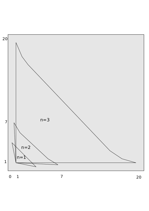
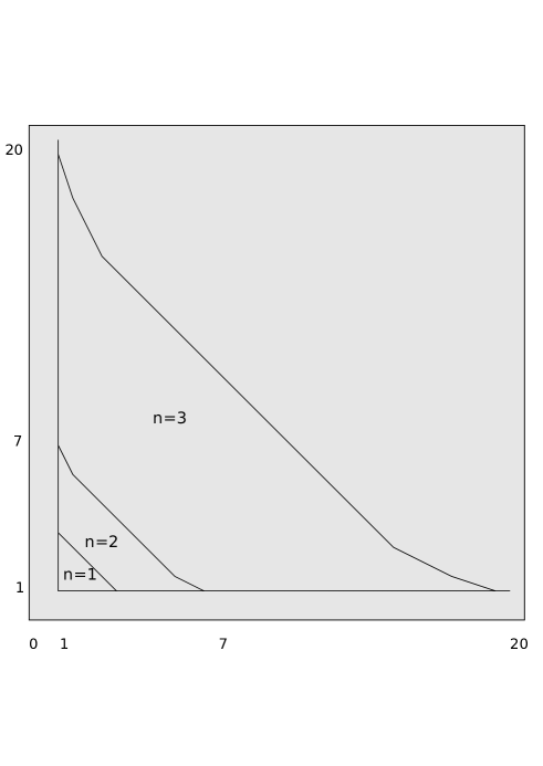
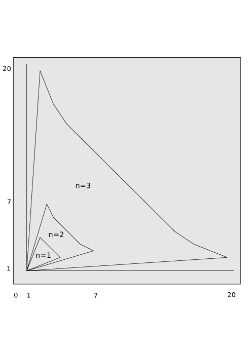
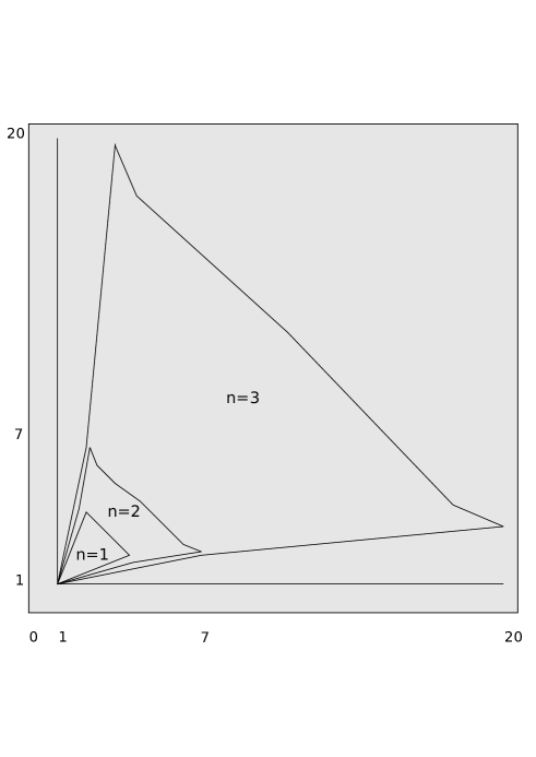
From the graph it appears that the solution space strictly increases with nn when ρ0\rho\geq 0. However, this is not true for ρ<0\rho<0.

8 Conclusion

In this article, we built upon existing methodologies that use relative entropy based ideas for incorporating mathematically specified views/constraints to a given financial model to arrive at a more accurate one, when the underlying random variables are light tailed. In the existing financial literature, these ideas have found many applications including in portfolio modeling, in model calibration and in ascertaining the pricing probability measure in incomplete markets. Our key contribution was to show that under technical conditions, using polynomial-divergence, such constraints may be uniquely incorporated even when the underlying random variables have fat tails. We also extended the proposed methodology to allow for constraints on marginal distributions of functions of underlying variables. This, in addition to the constraints on moments of functions of underlying random variables, traditionally considered for such problems. Here, we considered, both II-divergence and polynomial-divergence as objective.

We also specialized our results to the Markowitz portfolio modeling framework where multivariate Gaussian distribution is used to model asset returns. Here, we developed close form solutions for the updated posterior distribution. In case when there is a constraint that a marginal of a single portfolio of assets has a fat-tailed distribution, we showed that under the posterior distribution, marginal of all assets with non-zero correlation with this portfolio have similar fat-tailed distribution. This may be a reasonable and a simple way to incorporate realistic tail behavior in a portfolio of assets.

We also qualitatively compared the solution to the optimization problem in a simple setting of exponentially distributed prior when the objective function was II-divergence, polynomial-divergence and total variational distance. We found that in certain settings, II-divergence may put more mass in tails compared to polynomial-divergence, which may penalize tail deviation more. Finally, we numerically tested the proposed methodology on some simple examples.


Acknowledgement: The authors would like to thank Paul Glasserman for many directional suggestions as well as specific inputs on the manuscript that greatly helped this effort. We would also like to thank the Associate Editor and the referees for feedbacks that substantially improved the article.

9 Appendix: Proofs

Proof of Proposition 1 Recall that f(x)=α1(1+x)αf(x)=\frac{\alpha-1}{(1+x)^{\alpha}} for x0x\geq 0, and

fλM(x)=eλMxf(x)I[0,M](x)0MeλMxf(x)𝑑x{f}_{\lambda_{M}}(x)=\frac{e^{\lambda_{M}x}f(x)I_{[0,M]}(x)}{\int_{0}^{M}e^{\lambda_{M}x}f(x)dx}

where λM\lambda_{M} is the unique solution to 0Mxfλ(x)𝑑x=c\int_{0}^{M}x{f}_{\lambda}(x)\,dx=c.

We first show that λM0\lambda_{M}\rightarrow 0 as MM\rightarrow\infty. To this end, let

g(λ,M)=0Mxeλxf(x)𝑑x0Meλxf(x)𝑑x,M1,λ0.g(\lambda,M)=\frac{\int_{0}^{M}xe^{\lambda x}f(x)\,dx}{\int_{0}^{M}e^{\lambda x}f(x)\,dx}\,\,,M\geq 1,\,\lambda\geq 0.

We have

gλ\displaystyle\frac{\partial g}{\partial\lambda} =\displaystyle= (0Mx2eλxf(x)𝑑x)(0Meλxf(x)𝑑x)(0Mxeλxf(x)𝑑x)2(0Meλxf(x)𝑑x)2\displaystyle\frac{\left(\int_{0}^{M}x^{2}e^{\lambda x}f(x)\,dx\right)\left(\int_{0}^{M}e^{\lambda x}f(x)\,dx\right)-\left(\int_{0}^{M}xe^{\lambda x}f(x)\,dx\right)^{2}}{\left(\int_{0}^{M}e^{\lambda x}f(x)\,dx\right)^{2}}
=\displaystyle= 0Mx2(eλxf(x)0Meλxf(x)𝑑x)𝑑x(0Mx(eλxf(x)0Meλxf(x)𝑑x)𝑑x)2\displaystyle\int_{0}^{M}x^{2}\left(\frac{e^{\lambda x}f(x)}{\int_{0}^{M}e^{\lambda x}f(x)\,dx}\right)\,dx-\left(\int_{0}^{M}x\left(\frac{e^{\lambda x}f(x)}{\int_{0}^{M}e^{\lambda x}f(x)\,dx}\right)\,dx\right)^{2}
=\displaystyle= Eλ[X2](Eλ[X])2>0\displaystyle E_{\lambda}[X^{2}]-\left(E_{\lambda}[X]\right)^{2}>0

where EλE_{\lambda} is the expectation operator w.r.t density function fλf_{\lambda}.

Also

gM\displaystyle\frac{\partial g}{\partial M} =\displaystyle= (MeλMf(M))(0Meλxf(x)𝑑x)(0Mxeλxf(x)𝑑x)(eλMf(M)f(0))(0Meλxf(x)𝑑x)2\displaystyle\frac{\left(Me^{\lambda M}f(M)\right)\left(\int_{0}^{M}e^{\lambda x}f(x)\,dx\right)-\left(\int_{0}^{M}xe^{\lambda x}f(x)\,dx\right)\left(e^{\lambda M}f(M)-f(0)\right)}{\left(\int_{0}^{M}e^{\lambda x}f(x)\,dx\right)^{2}}
=\displaystyle= eλMf(M)0M(Mx)eλxf(x)𝑑x+f(0)0Meλxf(x)𝑑x(0Meλxf(x)𝑑x)2>0.\displaystyle\frac{e^{\lambda M}f(M)\int_{0}^{M}(M-x)e^{\lambda x}f(x)\,dx+f(0)\int_{0}^{M}e^{\lambda x}f(x)\,dx}{\left(\int_{0}^{M}e^{\lambda x}f(x)\,dx\right)^{2}}>0.

Since λM\lambda_{M} satisfies g(λM,M)=cg(\lambda_{M},M)=c, it follows that increasing MM leads to reduction in λM\lambda_{M}. That is, λM\lambda_{M} is a non-increasing function of MM.

Suppose that λMc1>0\lambda_{M}\downarrow c_{1}>0. Then c=g(λM,M)g(c1,M)c=g(\lambda_{M},M)\geq g(c_{1},M) for all MM. But since c1>0c_{1}>0 we have g(c1,M)g(c_{1},M)\rightarrow\infty as MM\rightarrow\infty, a contradiction. Hence, λM0\lambda_{M}\rightarrow 0 as MM\rightarrow\infty.

Next, since

0Mlog(fλ(x)f(x))fλ(x)𝑑x=λ0Mxfλ(x)𝑑xlog(0Meλxf(x)𝑑x),\int_{0}^{M}\log\left(\frac{f_{\lambda}(x)}{f(x)}\right)f_{\lambda}(x)\,dx=\lambda\int_{0}^{M}xf_{\lambda}(x)\,dx-\log\left(\int_{0}^{M}e^{\lambda x}f(x)\,dx\right),

we see that

0Mlog(fλM(x)f(x))fλM(x)𝑑x=λMclog(0MeλMxf(x)𝑑x).\int_{0}^{M}\log\left(\frac{f_{\lambda_{M}}(x)}{f(x)}\right)f_{\lambda_{M}}(x)\,dx=\lambda_{M}c-\log\left(\int_{0}^{M}e^{{\lambda_{M}}x}f(x)\,dx\right).

Hence, to prove that the LHS converges to zero as MM\rightarrow\infty, it suffices to show that
0MeλMxf(x)𝑑x1\int_{0}^{M}e^{\lambda_{M}x}f(x)\,dx\rightarrow 1 or that 0MeλMx(1+x)α𝑑x1α1\int_{0}^{M}\frac{e^{\lambda_{M}x}}{(1+x)^{\alpha}}\,dx\rightarrow\frac{1}{\alpha-1}.

Note that the constraint equation can be re-expressed as:

c=0MxfλM(x)𝑑x=0MxeλMx(1+x)α𝑑x0MeλMx(1+x)α𝑑x=0MeλMx(1+x)α1𝑑x0MeλMx(1+x)α𝑑x0MeλMx(1+x)α𝑑x=0MeλMx(1+x)α1𝑑x0MeλMx(1+x)α𝑑x1,c=\int_{0}^{M}xf_{\lambda_{M}}(x)\,dx=\frac{\int_{0}^{M}\frac{xe^{{\lambda_{M}}x}}{(1+x)^{\alpha}}\,dx}{\int_{0}^{M}\frac{e^{{\lambda_{M}}x}}{(1+x)^{\alpha}}\,dx}=\frac{\int_{0}^{M}\frac{e^{{\lambda_{M}}x}}{(1+x)^{\alpha-1}}\,dx-\int_{0}^{M}\frac{e^{{\lambda_{M}}x}}{(1+x)^{\alpha}}\,dx}{\int_{0}^{M}\frac{e^{{\lambda_{M}}x}}{(1+x)^{\alpha}}\,dx}=\frac{\int_{0}^{M}\frac{e^{{\lambda_{M}}x}}{(1+x)^{\alpha-1}}\,dx}{\int_{0}^{M}\frac{e^{{\lambda_{M}}x}}{(1+x)^{\alpha}}\,dx}-1,

or

0MeλMx(1+x)α1𝑑x0MeλMx(1+x)α𝑑x=1+c.\frac{\int_{0}^{M}\frac{e^{{\lambda_{M}}x}}{(1+x)^{\alpha-1}}\,dx}{\int_{0}^{M}\frac{e^{{\lambda_{M}}x}}{(1+x)^{\alpha}}\,dx}=1+c. (32)

Further, by integration by parts of the numerator, we observe that

0MeλMx(1+x)α1𝑑x=1λM(eλMM(1+M)α11+(α1)0MeλMx(1+x)α𝑑x).{\int_{0}^{M}\frac{e^{{\lambda_{M}}x}}{(1+x)^{\alpha-1}}\,dx}=\frac{1}{\lambda_{M}}\left(\frac{e^{\lambda_{M}M}}{(1+M)^{\alpha-1}}-1+(\alpha-1)\int_{0}^{M}\frac{e^{\lambda_{M}x}}{(1+x)^{\alpha}}\,dx\right).

From the above equation and (32), it follows that

0MeλMx(1+x)α𝑑x=eλMM(1+M)α11λM(c+1)(α1).\int_{0}^{M}\frac{e^{\lambda_{M}x}}{(1+x)^{\alpha}}\,dx=\frac{\frac{e^{\lambda_{M}M}}{(1+M)^{\alpha-1}}-1}{\lambda_{M}(c+1)-(\alpha-1)}. (33)

Since λM0\lambda_{M}\rightarrow 0, it suffices to show that

eλMM(1+M)α10.\frac{e^{\lambda_{M}M}}{(1+M)^{\alpha-1}}\rightarrow 0.

Suppose this is not true. Then, there exists an η>0\eta>0 and a sequence MiM_{i}\uparrow\infty such that eλMiMi(1+Mi)α1η\frac{e^{\lambda_{M_{i}}M_{i}}}{(1+M_{i})^{\alpha-1}}\geq\eta. Equation (32) may be re-expressed as:

0MeλMx(1+x)α1[11+c1+x]𝑑x=0\int_{0}^{M}\frac{e^{\lambda_{M}x}}{(1+x)^{\alpha-1}}\left[1-\frac{1+c}{1+x}\right]dx=0 (34)

Given an arbitrary K>0K>0, one can find an Mi1+2cM_{i}\geq 1+2c (so that 11+c1+x121-\frac{1+c}{1+x}\geq\frac{1}{2} when xMix\geq M_{i}) such that, for x[MiK,Mi]x\in[M_{i}-K,M_{i}]

eλMix(1+x)α1eλMi(MiK)(1+Mi)α1η2.\frac{e^{\lambda_{M_{i}}x}}{(1+x)^{\alpha-1}}\geq\frac{e^{\lambda_{M_{i}}(M_{i}-K)}}{(1+M_{i})^{\alpha-1}}\geq\frac{\eta}{2}.

Re-expressing the LHS of (34) evaluated at M=MiM=M_{i} as

0ceλMix(1+x)α1[11+c1+x]𝑑x+cMiKeλMix(1+x)α1[11+c1+x]𝑑x+MiKMieλMix(1+x)α1[11+c1+x]𝑑x,\int_{0}^{c}\frac{e^{\lambda_{M_{i}}x}}{(1+x)^{\alpha-1}}\left[1-\frac{1+c}{1+x}\right]dx+\int_{c}^{M_{i}-K}\frac{e^{\lambda_{M_{i}}x}}{(1+x)^{\alpha-1}}\left[1-\frac{1+c}{1+x}\right]dx+\int_{M_{i}-K}^{M_{i}}\frac{e^{\lambda_{M_{i}}x}}{(1+x)^{\alpha-1}}\left[1-\frac{1+c}{1+x}\right]dx,

we see that this is bounded from below by

c2eλMic+Kη/4.-c^{2}e^{\lambda_{M_{i}}c}+K\eta/4.

For sufficiently large KK, this is greater than zero providing the desired contradiction to (34).\Box


Proof of Theorem 2:   Let ξ=(1+βlλlgl)1/β𝑑μ\xi=\int\left(1+\beta\sum_{l}\lambda_{l}g_{l}\right)^{1/\beta}\,d\mu. and λ^l=(β+1)βλl/ξβ\hat{\lambda}_{l}=(\beta+1)\beta\lambda_{l}/\xi^{\beta}. Consider the Lagrangian (ν)\mathcal{L}(\nu) for 𝐎𝟐(β){\bf O_{2}}(\beta) defined as

(dνdμ)β+1𝑑μlλ^l(gl𝑑νcl).\int\left(\frac{d\nu}{d\mu}\right)^{\beta+1}\,d\mu-\sum_{l}\hat{\lambda}_{l}\left(\int g_{l}\,d\nu-c_{l}\right). (35)

We first argue that (ν)\mathcal{L}(\nu) is a convex function of ν\nu. Given that λlgl𝑑ν\lambda_{l}\int g_{l}\,d\nu are linear in ν\nu, it suffices to show that (dνdμ)β+1𝑑μ\int(\frac{d\nu}{d\mu})^{\beta+1}\,d\mu is a convex function of ν\nu.

Note that for 0s10\leq s\leq 1,

(d(sν1+(1s)ν2)dμ)β+1𝑑μ\int\left(\frac{d(s\nu_{1}+(1-s)\nu_{2})}{d\mu}\right)^{\beta+1}\,d\mu

equals

(sdν1dμ+(1s)dν2dμ)β+1𝑑μ\int\left(s\frac{d\nu_{1}}{d\mu}+(1-s)\frac{d\nu_{2}}{d\mu}\right)^{\beta+1}\,d\mu

which in turn is dominated by

[s(dν1dμ)β+1+(1s)(dν2dμ)β+1]𝑑μ\int\left[s\left(\frac{d\nu_{1}}{d\mu}\right)^{\beta+1}+(1-s)\left(\frac{d\nu_{2}}{d\mu}\right)^{\beta+1}\right]\,d\mu

which equals

s(dν1dμ)β+1𝑑μ+(1s)(dν2dμ)β+1𝑑μ.s\int\left(\frac{d\nu_{1}}{d\mu}\right)^{\beta+1}\,d\mu+(1-s)\int\left(\frac{d\nu_{2}}{d\mu}\right)^{\beta+1}\,d\mu.

Therefore, the Lagrangian (ν)\mathcal{L}(\nu) is a convex function of ν\nu.

We now prove that (ν)\mathcal{L}(\nu) is minimized at ν1\nu^{1}. For this, all we need to show is that we cannot improve by moving in any feasible direction away from ν1\nu^{1}. Since, ν1\nu^{1} satisfies all the constraints, the result then follows. We now show this.

Let ff denote dνdμ\frac{d\nu}{d\mu} and f1=dν1dμf^{1}=\frac{d\nu^{1}}{d\mu}. Note that (35) may be re-expressed as

(fβ+1lλ^lglf)𝑑μ+lλ^lcl.\int\left(f^{\beta+1}-\sum_{l}\hat{\lambda}_{l}g_{l}f\right)\,d\mu+\sum_{l}\hat{\lambda}_{l}c_{l}.

For any ν𝒫(μ)\nu\in\mathcal{P}(\mu) and t[0,1]t\in[0,1] consider the function

Gν(t)=((1t)ν1+tν).G_{\nu}(t)=\mathcal{L}\left((1-t)\nu^{1}+t\nu\right).

This in turn equals

[{(1t)f1+tf}β+1lλ^lgl{(1t)f1+tf}]𝑑μ+lλ^lcl.\int\left[\{(1-t)f^{1}+tf\}^{\beta+1}-\sum_{l}\hat{\lambda}_{l}g_{l}\{(1-t)f^{1}+tf\}\right]\,d\mu+\sum_{l}\hat{\lambda}_{l}c_{l}.

We now argue that ddtt=0Gν(t)=0{\frac{d}{dt}}_{t=0}G_{\nu}(t)=0. Then from this and convexity of \mathcal{L}, the result follows.

To see this, note that ddtt=0Gν(t){\frac{d}{dt}}_{t=0}G_{\nu}(t) equals

{(β+1)(f1)βlλ^lgl}(ff1)𝑑μ.\int\left\{(\beta+1)(f^{1})^{\beta}-\sum_{l}\hat{\lambda}_{l}g_{l}\right\}(f-f^{1})\,d\mu. (36)

Due to the definition of f1f_{1} and λ^i\hat{\lambda}_{i}, it follows that the term inside the braces in the integrand in (36) is a constant. Since both ν1\nu^{1} and ν\nu are probability measures, therefore ddtt=0Gν(t)=0{\frac{d}{dt}}_{t=0}G_{\nu}(t)=0 and the result follows.\Box


Proof of Theorem 3:   Let AA denote the set of all strongly feasible solutions to (12). Consider the following set of equations:

gj(1+βl=1kθl(glcl))1β𝑑μ(1+βl=1kθl(glcl))1β𝑑μ=cjforj=1,2,,k.\frac{\int g_{j}\left(1+\beta\sum_{l=1}^{k}\theta_{l}(g_{l}-c_{l})\right)^{\frac{1}{\beta}}\,d\mu}{\int\left(1+\beta\sum_{l=1}^{k}\theta_{l}(g_{l}-c_{l})\right)^{\frac{1}{\beta}}\,d\mu}=c_{j}\,\,\,\text{for}\,\,j=1,2,\ldots,k. (37)

We say that 𝜽=(θ1,θ2,,θk)\mbox{\boldmath{$\theta$}}=(\theta_{1},\theta_{2},\ldots,\theta_{k}) is a strongly feasible solution to (37) if it solves (37), and lies in the set:

{𝜽k1+βl=1kθl(glθl)0a.e.μ,(1+βl=1kθl(glcl))1β+1𝑑μ<andβl=1kθlcl<1}.\left\{\mbox{\boldmath{$\theta$}}\in\mathbb{R}^{k}\mid 1+\beta\sum_{l=1}^{k}\theta_{l}(g_{l}-\theta_{l})\geq 0\,\,a.e.\mu,\int(1+\beta\sum_{l=1}^{k}\theta_{l}(g_{l}-c_{l}))^{\frac{1}{\beta}+1}d\mu<\infty\,\,\text{and}\,\beta\sum_{l=1}^{k}\theta_{l}c_{l}<1\right\}.

Let BB denote the set of all strongly feasible solutions to (37).

Let ϕ:AB\phi:A\rightarrow B and ψ:BA\psi:B\rightarrow A be the mappings defined by

ϕ(𝝀)=(λ11+βl=1kλlcl,λ21+βl=1kλlcl,,λk1+βl=1kλlcl)\phi(\mbox{\boldmath{$\lambda$}})=\left(\frac{\lambda_{1}}{1+\beta\sum_{l=1}^{k}\lambda_{l}c_{l}},\frac{\lambda_{2}}{1+\beta\sum_{l=1}^{k}\lambda_{l}c_{l}},\ldots,\frac{\lambda_{k}}{1+\beta\sum_{l=1}^{k}\lambda_{l}c_{l}}\right)

and

ψ(𝜽)=(θ11βl=1kθlcl,θ21βl=1kθlcl,,θk1βl=1kθlcl).\psi(\mbox{\boldmath{$\theta$}})=\left(\frac{\theta_{1}}{1-\beta\sum_{l=1}^{k}\theta_{l}c_{l}},\frac{\theta_{2}}{1-\beta\sum_{l=1}^{k}\theta_{l}c_{l}},\ldots,\frac{\theta_{k}}{1-\beta\sum_{l=1}^{k}\theta_{l}c_{l}}\right).

It is easily checked that mapping ϕ\phi is a bijection with inverse ψ\psi. Note that if 𝝀A\mbox{\boldmath{$\lambda$}}\in A, then ϕ(𝝀)B\phi(\mbox{\boldmath{$\lambda$}})\in B. To see this, simply divide the numerator and the denominator in (12) by (1+βl=1kλlcl)1/β(1+\beta\sum_{l=1}^{k}\lambda_{l}c_{l})^{1/\beta}. Conversely, if 𝜽B\mbox{\boldmath{$\theta$}}\in B, then ψ(𝜽)A\psi(\mbox{\boldmath{$\theta$}})\in A. To see this, divide the numerator and the denominator in (37) by (1βl=1kθlcl)1/β(1-\beta\sum_{l=1}^{k}\theta_{l}c_{l})^{1/\beta}.

Therefore, its suffices to prove uniqueness of strongly feasible solutions to (37). To this end, consider the function G:B+G:B\rightarrow\mathbb{R}^{+}:

G(𝜽)=(1+βl=1kθl(glcl))1β+1𝑑μ.G(\mbox{\boldmath{$\theta$}})=\int\left(1+\beta\sum_{l=1}^{k}\theta_{l}(g_{l}-c_{l})\right)^{\frac{1}{\beta}+1}\,d\mu.

Then,

Gθi=(1+β)(gici)(1+βl=1kθl(glcl))1β𝑑μ.\frac{\partial G}{\partial\theta_{i}}=\left({1+\beta}\right)\int(g_{i}-c_{i})\left(1+\beta\sum_{l=1}^{k}\theta_{l}(g_{l}-c_{l})\right)^{\frac{1}{\beta}}\,d\mu. (38)

and

2Gθjθi=β(1+β)(gici)(gjcj)(1+βl=1kθl(glcl))1β1𝑑μ.\frac{\partial^{2}G}{\partial\theta_{j}\partial\theta_{i}}={\beta}({1+\beta})\int(g_{i}-c_{i})(g_{j}-c_{j})\left(1+\beta\sum_{l=1}^{k}\theta_{l}(g_{l}-c_{l})\right)^{\frac{1}{\beta}-1}\,d\mu\,.

We see that the last integral can be written as Eθ[(gici)(gjcj)]E_{\theta}[(g_{i}-c_{i})(g_{j}-c_{j})] times a positive constant independent of ii and jj, where EθE_{\theta} denotes expectation under the measure

(1+βl=1kθl(glcl))1β1dμ(1+βl=1kθl(glcl))1β1𝑑μ.\frac{\left(1+\beta\sum_{l=1}^{k}\theta_{l}(g_{l}-c_{l})\right)^{\frac{1}{\beta}-1}\,d\mu}{\int\left(1+\beta\sum_{l=1}^{k}\theta_{l}(g_{l}-c_{l})\right)^{\frac{1}{\beta}-1}\,d\mu}.

Now from the identity

Eθ[(gici)(gjcj)]=Covθ[gi,gj]+(Eθ[gi]ci)(Eθ[gj]cj)E_{\theta}[(g_{i}-c_{i})(g_{j}-c_{j})]=\text{Cov}_{\theta}[g_{i},g_{j}]+\left(E_{\theta}[g_{i}]-c_{i}\right)\left(E_{\theta}[g_{j}]-c_{j}\right)

and the assumption on gig_{i}’s it follows that the Hessian of the function GG is positive definite. Thus, GG is strictly convex in its domain of definition, that is in BB. Therefore if a solution to the equation

(Gθ1,Gθ2,,Gθk)=0\left(\frac{\partial G}{\partial\theta_{1}},\frac{\partial G}{\partial\theta_{2}},\ldots,\frac{\partial G}{\partial\theta_{k}}\right)=0 (39)

exists in BB, then it is unique. From (38) it follows that the set of equations given by (39) and (37) are equivalent. \Box


Proof of Proposition 3: First assume that 𝐜𝒞{\bf c}\notin\mathcal{C} so that 𝐎𝟐(β,𝐜){\bf O_{2}}(\beta,{\bf c}) has no solution. Note that 𝐜𝟎{\bf c_{0}} may not belong to 𝒞\mathcal{C} so that 𝐎𝟐(β,𝐜𝟎){\bf O_{2}}(\beta,{\bf c_{0}}) may also not have a solution. Let B(x,r)B(x,r) denote the open ball centered at xx and radius rr with respect to the metric dd defined at Section 3.3. For arbitrary ε>0\varepsilon>0, let 𝐜εB(𝐜𝟎,ε)𝒞{\bf c}_{\varepsilon}\in B({\bf c_{0}},\varepsilon)\bigcap\mathcal{C}. Then 𝐎𝟐(β,𝐜ε){\bf O_{2}}(\beta,{\bf c}_{\varepsilon}) has a solution, say νε\nu_{\varepsilon} and let λ(ϵ){\bf\lambda}(\epsilon) denote the associated parameters. It follows that (λ(ϵ),𝐜ε𝐜)({\bf\lambda}(\epsilon),{\bf c}_{\varepsilon}-{\bf c}) is feasible for 𝐎~𝟐(β,t,𝐜){\bf\tilde{O}_{2}}(\beta,t,{\bf c}) for any tt. Since (λt,𝐲t)({{\bf\lambda}_{t}},{\bf y}_{t}) is a solution to 𝐎~𝟐(β,t,𝐜){\bf\tilde{O}_{2}}(\beta,t,{\bf c}), we have

Iβ(νλt||μ)+1ti=1k𝐲t(i)2wiIβ(νε||μ)+1ti=1k(𝐜ε(i)𝐜(i))2wi,I_{\beta}(\nu_{\lambda_{t}}||\mu)+\frac{1}{t}\sum_{i=1}^{k}\frac{{\bf y}_{t}(i)^{2}}{w_{i}}\leq I_{\beta}(\nu_{\varepsilon}||\mu)+\frac{1}{t}\sum_{i=1}^{k}\frac{\left({\bf c}_{\varepsilon}(i)-{\bf c}(i)\right)^{2}}{w_{i}},

or

Iβ(νλt||μ)+1td(𝐜,𝐜+𝐲t)Iβ(νε||μ)+1td(𝐜,𝐜ε).I_{\beta}(\nu_{\lambda_{t}}||\mu)+\frac{1}{t}d({\bf c},{\bf c}+{\bf y}_{t})\leq I_{\beta}(\nu_{\varepsilon}||\mu)+\frac{1}{t}d({\bf c},{\bf c}_{\varepsilon}).

But, by triangle inequality and definition of 𝐜ε{\bf c}_{\varepsilon}, it follows that

d(𝐜,𝐜ε)d(𝐜,𝐜𝟎)+d(𝐜𝟎,𝐜ε)d(𝐜,𝐜𝟎)+ε.d({\bf c},{\bf c}_{\varepsilon})\leq d({\bf c},{\bf c_{0}})+d({\bf c_{0}},{\bf c}_{\varepsilon})\leq d({\bf c},{\bf c_{0}})+\varepsilon.

Therefore,

Iβ(νλt||μ)+1td(𝐜,𝐜+𝐲t)Iβ(νε||μ)+1td(𝐜,𝐜𝟎)+εt.I_{\beta}(\nu_{\lambda_{t}}||\mu)+\frac{1}{t}d({\bf c},{\bf c}+{\bf y}_{t})\leq I_{\beta}(\nu_{\varepsilon}||\mu)+\frac{1}{t}d({\bf c},{\bf c_{0}})+\frac{\varepsilon}{t}.

Since, Iβ(νλt||μ)0I_{\beta}(\nu_{\lambda_{t}}||\mu)\geq 0 we have

d(𝐜,𝐜+𝐲t)tIβ(νε||μ)+d(𝐜,𝐜𝟎)+ε.d({\bf c},{\bf c}+{\bf y}_{t})\leq tI_{\beta}(\nu_{\varepsilon}||\mu)+d({\bf c},{\bf c_{0}})+\varepsilon.

Since tt can be chosen arbitrarily small, we conclude that

d(𝐜,𝐜+𝐲t)d(𝐜,𝐜𝟎)+2ε.d({\bf c},{\bf c}+{\bf y}_{t})\leq d({\bf c},{\bf c_{0}})+2\varepsilon. (40)

Now, since 𝐜+𝐲t𝒞{\bf c}+{\bf y}_{t}\in\mathcal{C}, by definition of 𝐜𝟎{\bf c_{0}} we have

d(𝐜,𝐜+𝐲t)d(𝐜,𝐜𝟎).d({\bf c},{\bf c}+{\bf y}_{t})\geq d({\bf c},{\bf c_{0}}).

Together with inequality (40), we have,

limt0d(𝐜,𝐜+𝐲t)=d(𝐜,𝐜𝟎).\lim_{t\downarrow 0}d({\bf c},{\bf c}+{\bf y}_{t})=d({\bf c},{\bf c_{0}}).

If 𝐜𝒞{\bf c}\in\mathcal{C} then 𝐎𝟐(β,𝐜){\bf O_{2}}(\beta,{\bf c}) has a solution. Then the above analysis simplifies: 𝐜𝟎=𝐜{\bf c_{0}}={\bf c} and each 𝐜ε{\bf c}_{\varepsilon} can be taken to be equal to 𝐜{\bf c}. We conclude that

limt0d(𝐜,𝐜+𝐲t)=0\lim_{t\downarrow 0}d({\bf c},{\bf c}+{\bf y}_{t})=0

or 𝐲t0{\bf y}_{t}\rightarrow 0. \Box


Proof of Theorem 4:   In view of (18), we may fix the marginal distribution of 𝕏\mathbb{X} to be g(𝕩)g(\mathbb{x}) and re-express the objective as

minf~(|𝕩)𝒫(f(|𝕩)),𝕩𝕩,𝕪log(f~(𝕪|𝕩)f(𝕪|𝕩))f~(𝕪|𝕩)g(𝕩)𝑑𝕪𝑑𝕩+𝕩log(g(𝕩)f(𝕩))g(𝕩)𝑑𝕩.\min_{\tilde{f}(\cdot|\mathbb{x})\in{\cal P}({f}(\cdot|\mathbb{x})),\forall\mathbb{x}}\int_{\mathbb{x},\mathbb{y}}\log\left(\frac{\tilde{f}(\mathbb{y}|\mathbb{x})}{f(\mathbb{y}|\mathbb{x})}\right)\tilde{f}(\mathbb{y}|\mathbb{x})g(\mathbb{x})d\mathbb{y}d\mathbb{x}+\int_{\mathbb{x}}\log\left(\frac{g(\mathbb{x})}{f(\mathbb{x})}\right)g(\mathbb{x})d\mathbb{x}\,.

The second integral is a constant and can be dropped from the objective. The first integral may in turn be expressed as

𝕩minf~(|𝕩)𝒫(f(|𝕩))(𝕪logf~(𝕪|𝕩)f(𝕪|𝕩)f~(𝕪|𝕩)𝑑𝕪)g(𝕩)𝑑𝕩.\int_{\mathbb{x}}\min_{\tilde{f}(\cdot|\mathbb{x})\in{\cal P}({f}(\cdot|\mathbb{x}))}\left(\int_{\mathbb{y}}\log\frac{\tilde{f}(\mathbb{y}|\mathbb{x})}{f(\mathbb{y}|\mathbb{x})}\tilde{f}(\mathbb{y}|\mathbb{x})d\mathbb{y}\right)g(\mathbb{x})d\mathbb{x}\,.

Similarly the moment constraints can be re-expressed as

𝕩,𝕪hi(𝕩,𝕪)f~(𝕪|𝕩)g(𝕩)𝑑𝕩𝑑𝕪=ci,i=1,2,,k\int_{\mathbb{x},\mathbb{y}}h_{i}(\mathbb{x},\mathbb{y})\tilde{f}(\mathbb{y}|\mathbb{x})g(\mathbb{x})d\mathbb{x}d\mathbb{y}=c_{i},\,\,\,i=1,2,...,k

or

𝕩(𝕪hi(𝕩,𝕪)f~(𝕪|𝕩)𝑑𝕪)g(𝕩)𝑑𝕩=ci,i=1,2,,k.\int_{\mathbb{x}}\left(\int_{\mathbb{y}}h_{i}(\mathbb{x},\mathbb{y})\tilde{f}(\mathbb{y}|\mathbb{x})d\mathbb{y}\right)g(\mathbb{x})d\mathbb{x}=c_{i},\,\,\,i=1,2,...,k\,.

Then, the Lagrangian for this kk constraint problem is,

𝕩[minf~(|𝕩)𝒫(f(|𝕩))𝕪(logf~(𝕪|𝕩)f(𝕪|𝕩)f~(𝕪|𝕩)iδihi(𝕩,𝕪)f~(𝕪|𝕩))𝑑𝕪]g(𝕩)𝑑𝕩+iδici.\int_{\mathbb{x}}\left[\min_{\tilde{f}(\cdot|\mathbb{x})\in{\cal P}({f}(\cdot|\mathbb{x}))}\int_{\mathbb{y}}\left(\log\frac{\tilde{f}(\mathbb{y}|\mathbb{x})}{f(\mathbb{y}|\mathbb{x})}\tilde{f}(\mathbb{y}|\mathbb{x})-\sum_{i}\delta_{i}h_{i}(\mathbb{x},\mathbb{y})\tilde{f}(\mathbb{y}|\mathbb{x})\right)d\mathbb{y}\right]g(\mathbb{x})d\mathbb{x}+\sum_{i}\delta_{i}c_{i}\,.

Note that by Theorem (1)

minf~(|𝕩)𝒫(f(|𝕩))𝕪(logf~(𝕪|𝕩)f(𝕪|𝕩)f~(𝕪|𝕩)iδihi(𝕩,𝕪)f~(𝕪|𝕩))𝑑y\min_{\tilde{f}(\cdot|\mathbb{x})\in{\cal P}({f}(\cdot|\mathbb{x}))}\int_{\mathbb{y}}\left(\log\frac{\tilde{f}(\mathbb{y}|\mathbb{x})}{f(\mathbb{y}|\mathbb{x})}\tilde{f}(\mathbb{y}|\mathbb{x})-\sum_{i}\delta_{i}h_{i}(\mathbb{x},\mathbb{y})\tilde{f}(\mathbb{y}|\mathbb{x})\right)dy

has the solution

f~𝜹(𝕪|𝕩)=exp(iδihi(𝕩,𝕪))f(𝕪|𝕩)𝕪exp(iδihi(𝕩,𝕪))f(𝕪|𝕩)𝑑𝕪=exp(iδihi(𝕩,𝕪))f(𝕩,𝕪)𝕪exp(iδihi(𝕩,𝕪))f(𝕩,𝕪)𝑑𝕪,\tilde{f}_{\mbox{\boldmath{$\delta$}}}(\mathbb{y}|\mathbb{x})=\frac{\exp(\sum_{i}\delta_{i}h_{i}(\mathbb{x},\mathbb{y})){f}(\mathbb{y}|\mathbb{x})}{\int_{\mathbb{y}}\exp(\sum_{i}\delta_{i}h_{i}(\mathbb{x},\mathbb{y})){f}(\mathbb{y}|\mathbb{x})d\mathbb{y}}=\frac{\exp(\sum_{i}\delta_{i}h_{i}(\mathbb{x},\mathbb{y})){f}(\mathbb{x},\mathbb{y})}{\int_{\mathbb{y}}\exp(\sum_{i}\delta_{i}h_{i}(\mathbb{x},\mathbb{y})){f}(\mathbb{x},\mathbb{y})d\mathbb{y}},

where we write 𝜹\delta for (δ1,δ2,,δk)(\delta_{1},\delta_{2},\ldots,\delta_{k}). Now taking 𝜹=𝝀\mbox{\boldmath{$\delta$}}=\mbox{\boldmath{$\lambda$}}, it follows from Assumption 3 that f𝝀(𝕩,𝕪)=f~𝝀(𝕪|𝕩)g(𝕩)f_{\mbox{\boldmath{$\lambda$}}}(\mathbb{x},\mathbb{y})=\tilde{f}_{\mbox{\boldmath{$\lambda$}}}(\mathbb{y}|\mathbb{x})g(\mathbb{x}) is a solution to 𝐎𝟑.{\bf O_{3}}\,.\Box


Proof of Theorem 5:   Let F:kF:\mathbb{R}^{k}\rightarrow\mathbb{R} be a function defined as

F(𝝀)=𝕩log(𝕪exp(lλlhl(𝕩,𝕪))f(𝕪|𝕩)𝑑𝕪)g(𝕩)𝑑𝕩lλlcl.F(\mbox{\boldmath{$\lambda$}})=\int_{\mathbb{x}}\log\left(\int_{\mathbb{y}}exp\left(\sum_{l}\lambda_{l}h_{l}(\mathbb{x},\mathbb{y})\right)f(\mathbb{y}|\mathbb{x})d\mathbb{y}\right)g(\mathbb{x})d\mathbb{x}-\sum_{l}\lambda_{l}c_{l}.

Then,

Fλi\displaystyle\frac{\partial F}{\partial\lambda_{i}} =\displaystyle= 𝕩(𝕪hi(𝕩,𝕪)exp(lλlhl(𝕩,𝕪))f(𝕪|𝕩)𝑑𝕪𝕪exp(lλlhl(𝕩,𝕪))f(𝕪|𝕩)𝑑𝕪)g(𝕩)𝑑𝕩ci\displaystyle\int_{\mathbb{x}}\left(\frac{\int_{\mathbb{y}}h_{i}(\mathbb{x},\mathbb{y})exp\left(\sum_{l}\lambda_{l}h_{l}(\mathbb{x},\mathbb{y})\right)f(\mathbb{y}|\mathbb{x})d\mathbb{y}}{\int_{\mathbb{y}}exp\left(\sum_{l}\lambda_{l}h_{l}(\mathbb{x},\mathbb{y})\right)f(\mathbb{y}|\mathbb{x})d\mathbb{y}}\right)g(\mathbb{x})d\mathbb{x}-c_{i}
=\displaystyle= 𝕩(𝕪hi(𝕩,𝕪)exp(lλlhl(𝕩,𝕪))f(𝕪|𝕩)𝕪exp(lλlhl(𝕩,𝕪))f(𝕪|𝕩)𝑑𝕪𝑑𝕪)g(𝕩)𝑑𝕩ci\displaystyle\int_{\mathbb{x}}\left(\int_{\mathbb{y}}h_{i}(\mathbb{x},\mathbb{y})\frac{exp\left(\sum_{l}\lambda_{l}h_{l}(\mathbb{x},\mathbb{y})\right)f(\mathbb{y}|\mathbb{x})}{\int_{\mathbb{y}}exp\left(\sum_{l}\lambda_{l}h_{l}(\mathbb{x},\mathbb{y})\right)f(\mathbb{y}|\mathbb{x})d\mathbb{y}}\,d\mathbb{y}\right)g(\mathbb{x})d\mathbb{x}-c_{i}
=\displaystyle= 𝕩(𝕪hi(𝕩,𝕪)f𝝀(𝕪|𝕩)𝑑𝕪)g(𝕩)𝑑𝕩ci\displaystyle\int_{\mathbb{x}}\left(\int_{\mathbb{y}}h_{i}(\mathbb{x},\mathbb{y})f_{\mbox{\boldmath{$\lambda$}}}(\mathbb{y}|\mathbb{x})d\mathbb{y}\right)g(\mathbb{x})d\mathbb{x}-c_{i}
=\displaystyle= 𝕩𝕪hi(𝕩,𝕪)f𝝀(𝕩,𝕪)𝑑𝕩𝑑𝕪ci\displaystyle\int_{\mathbb{x}}\int_{\mathbb{y}}h_{i}(\mathbb{x},\mathbb{y})f_{\mbox{\boldmath{$\lambda$}}}(\mathbb{x},\mathbb{y})d\mathbb{x}d\mathbb{y}-c_{i}
=\displaystyle= E𝝀[hi(𝕏,𝕐)]ci.\displaystyle E_{\mbox{\boldmath{$\lambda$}}}[h_{i}(\mathbb{X},\mathbb{Y})]-c_{i}.

Hence the set of equations given by (20) is equivalent to:

(Fλ1,Fλ2,,Fλk)=0.\left(\frac{\partial F}{\partial\lambda_{1}},\frac{\partial F}{\partial\lambda_{2}},\ldots,\frac{\partial F}{\partial\lambda_{k}}\right)=0\,. (41)

Since

λjf𝝀(𝕪|𝕩)=hj(𝕩,𝕪)f𝝀(𝕪|𝕩)(𝕪hj(𝕩,𝕪)f𝝀(𝕪|𝕩)𝑑𝕪)×f𝝀(𝕪|𝕩),\frac{\partial}{\partial\lambda_{j}}f_{\mbox{\boldmath{$\lambda$}}}(\mathbb{y}|\mathbb{x})=h_{j}(\mathbb{x},\mathbb{y})f_{\mbox{\boldmath{$\lambda$}}}(\mathbb{y}|\mathbb{x})-\left(\int_{\mathbb{y}}h_{j}(\mathbb{x},\mathbb{y})f_{\mbox{\boldmath{$\lambda$}}}(\mathbb{y}|\mathbb{x})d\mathbb{y}\right)\times f_{\mbox{\boldmath{$\lambda$}}}(\mathbb{y}|\mathbb{x}),

we have

2Fλjλi\displaystyle\frac{\partial^{2}F}{\partial\lambda_{j}\partial\lambda_{i}} =\displaystyle= 𝕩(𝕪hi(𝕩,𝕪)λjf𝝀(𝕪|𝕩)𝑑𝕪)g(𝕩)𝑑𝕩\displaystyle\int_{\mathbb{x}}\left(\int_{\mathbb{y}}h_{i}(\mathbb{x},\mathbb{y})\frac{\partial}{\partial\lambda_{j}}f_{\mbox{\boldmath{$\lambda$}}}(\mathbb{y}|\mathbb{x})\,d\mathbb{y}\right)g(\mathbb{x})\,d\mathbb{x}
=\displaystyle= 𝕩(𝕪hi(𝕩,𝕪)hj(𝕩,𝕪)f𝝀(𝕪|𝕩)𝑑𝕪)g(𝕩)𝑑𝕩\displaystyle\int_{\mathbb{x}}\left(\int_{\mathbb{y}}h_{i}(\mathbb{x},\mathbb{y})h_{j}(\mathbb{x},\mathbb{y})f_{\mbox{\boldmath{$\lambda$}}}(\mathbb{y}|\mathbb{x})d\mathbb{y}\right)g(\mathbb{x})d\mathbb{x}
𝕩(𝕪hj(𝕩,𝕪)f𝝀(𝕪|𝕩)𝑑𝕪)(𝕪hi(𝕩,𝕪)f𝝀(𝕪|𝕩)𝑑𝕪)g(𝕩)𝑑𝕩\displaystyle-\int_{\mathbb{x}}\left(\int_{\mathbb{y}}h_{j}(\mathbb{x},\mathbb{y})f_{\mbox{\boldmath{$\lambda$}}}(\mathbb{y}|\mathbb{x})d\mathbb{y}\right)\left(\int_{\mathbb{y}}h_{i}(\mathbb{x},\mathbb{y})f_{\mbox{\boldmath{$\lambda$}}}(\mathbb{y}|\mathbb{x})d\mathbb{y}\right)g(\mathbb{x})d\mathbb{x}
=\displaystyle= Eg(𝕩)[E𝝀[hi(𝕏,𝕐)hj(𝕏,𝕐)𝕏]]Eg(𝕩)[E𝝀[hj(𝕏,𝕐)𝕏]×E𝝀[hi(𝕏,𝕐)𝕏]]\displaystyle E_{g(\mathbb{x})}\left[E_{\mbox{\boldmath{$\lambda$}}}[h_{i}(\mathbb{X},\mathbb{Y})h_{j}(\mathbb{X},\mathbb{Y})\mid\mathbb{X}]\right]-E_{g(\mathbb{x})}\left[E_{\mbox{\boldmath{$\lambda$}}}[h_{j}(\mathbb{X},\mathbb{Y})\mid\mathbb{X}]\times E_{\mbox{\boldmath{$\lambda$}}}[h_{i}(\mathbb{X},\mathbb{Y})\mid\mathbb{X}]\right]
=\displaystyle= Eg(𝕩)[Cov𝝀[hi(𝕏,𝕐),hj(𝕏,𝕐)𝕏]]\displaystyle E_{g(\mathbb{x})}\left[\text{Cov}_{\mbox{\boldmath{$\lambda$}}}[h_{i}(\mathbb{X},\mathbb{Y}),h_{j}(\mathbb{X},\mathbb{Y})\mid\mathbb{X}]\right]

Where Eg(𝕩)E_{g(\mathbb{x})} denote expectation with respect to the density function g(𝕩)g(\mathbb{x}). By our assumption, it follows that the Hessian of FF is positive definite. Thus, the function FF is strictly convex in k\mathbb{R}^{k}. Therefore if there exist a solution to (41), then it is unique. Since (41) is equivalent to (20), the theorem follows.\Box


Proof of Theorem 6:   Fixing the marginal of 𝕏\mathbb{X} to be g(𝕩)g(\mathbb{x}) we express the objective as

minf~(|𝕩)𝒫(f(|𝕩)),𝕩𝕩,𝕪(f~(𝕪|𝕩)g(𝕩)f(𝕪|𝕩)f(𝕩))βf~(𝕪|𝕩)g(𝕩)𝑑𝕪𝑑𝕩.\min_{\tilde{f}(\cdot|\mathbb{x})\in{\cal P}(f(\cdot|\mathbb{x})),\forall\mathbb{x}}\int_{\mathbb{x},\mathbb{y}}\left(\frac{\tilde{f}(\mathbb{y}|\mathbb{x})g(\mathbb{x})}{f(\mathbb{y}|\mathbb{x})f(\mathbb{x})}\right)^{\beta}\tilde{f}(\mathbb{y}|\mathbb{x})g(\mathbb{x})d\mathbb{y}d\mathbb{x}\,.

This may in turn be expressed as

𝕩minf~(|𝕩)𝒫(f(|𝕩))(𝕪(f~(𝕪|𝕩)f(𝕪|𝕩))βf~(𝕪|𝕩)𝑑𝕪)(g(𝕩)f(𝕩))βg(𝕩)𝑑𝕩.\int_{\mathbb{x}}\min_{\tilde{f}(\cdot|\mathbb{x})\in{\cal P}(f(\cdot|\mathbb{x}))}\left(\int_{\mathbb{y}}\left(\frac{\tilde{f}(\mathbb{y}|\mathbb{x})}{f(\mathbb{y}|\mathbb{x})}\right)^{\beta}\tilde{f}(\mathbb{y}|\mathbb{x})d\mathbb{y}\right)\left(\frac{g(\mathbb{x})}{f(\mathbb{x})}\right)^{\beta}g(\mathbb{x})d\mathbb{x}\,.

Similarly, the moment constraints can be re-expressed as

𝕩(𝕪hi(𝕩,𝕪)(f(𝕩)g(𝕩))βf~(𝕪|𝕩)𝑑𝕪)(g(𝕩)f(𝕩))βg(𝕩)𝑑𝕩=ci,i=1,2,,k.\int_{\mathbb{x}}\left(\int_{\mathbb{y}}h_{i}(\mathbb{x},\mathbb{y})\left(\frac{f(\mathbb{x})}{g(\mathbb{x})}\right)^{\beta}\tilde{f}(\mathbb{y}|\mathbb{x})d\mathbb{y}\right)\left(\frac{g(\mathbb{x})}{f(\mathbb{x})}\right)^{\beta}g(\mathbb{x})d\mathbb{x}=c_{i},\,\,\,i=1,2,...,k\,.

Then, the Lagrangian for this kk constraint problem is, up to the constant iδici\sum_{i}\delta_{i}c_{i},

𝕩[minf~(|𝕩)𝒫(f(|𝕩))𝕪((f~(𝕪|𝕩)f(𝕪|𝕩))βf~(𝕪|𝕩)iδihi(𝕩,𝕪)(f(𝕩)g(𝕩))βf~(𝕪|𝕩))𝑑𝕪](g(𝕩)f(𝕩))βg(𝕩)𝑑𝕩.\int_{\mathbb{x}}\left[\min_{\tilde{f}(\cdot|\mathbb{x})\in{\cal P}(f(\cdot|\mathbb{x}))}\int_{\mathbb{y}}\left(\left(\frac{\tilde{f}(\mathbb{y}|\mathbb{x})}{f(\mathbb{y}|\mathbb{x})}\right)^{\beta}\tilde{f}(\mathbb{y}|\mathbb{x})-\sum_{i}\delta_{i}h_{i}(\mathbb{x},\mathbb{y})\left(\frac{f(\mathbb{x})}{g(\mathbb{x})}\right)^{\beta}\tilde{f}(\mathbb{y}|\mathbb{x})\right)d\mathbb{y}\right]\left(\frac{g(\mathbb{x})}{f(\mathbb{x})}\right)^{\beta}g(\mathbb{x})d\mathbb{x}\,.

By Theorem (2), the inner minimization has the solution f𝜹,β(𝕪|𝕩)f_{\mbox{\boldmath{$\delta$}},\beta}(\mathbb{y}|\mathbb{x}). Now taking 𝜹=𝝀\mbox{\boldmath{$\delta$}}=\mbox{\boldmath{$\lambda$}}, it follows from Assumption (4) that f𝝀,β(𝕩,𝕪)=f𝝀,β(𝕪|𝕩)g(𝕩)f_{\mbox{\boldmath{$\lambda$}},\beta}(\mathbb{x},\mathbb{y})=f_{\mbox{\boldmath{$\lambda$}},\beta}(\mathbb{y}|\mathbb{x})g(\mathbb{x}) is the solution to 𝐎𝟒(β){\bf O_{4}}(\beta). \Box


Proof of Proposition 2:   In view of Assumption (2), we note that 1+λng(x)01+\frac{\lambda}{n}g(x)\geq 0 for all x0x\geq 0 if λ0\lambda\geq 0. By Theorem (2), the probability distribution minimizing the polynomial-divergence (with β=1/n\beta=1/n) w.r.t. ff is given by:

f~(x)=(1+λng(x))nf(x)c,x0,\tilde{f}(x)=\frac{\left(1+\frac{\lambda}{n}g(x)\right)^{n}f(x)}{c}\,\,,x\geq 0,

where

c=0(1+λng(x))nf(x)𝑑x=k=0nnk(nk)E[g(X)k]λk.c=\int_{0}^{\infty}\left(1+\frac{\lambda}{n}g(x)\right)^{n}f(x)\,dx=\sum_{k=0}^{n}n^{-k}\binom{n}{k}E[g(X)^{k}]\lambda^{k}.

From the constraint equation we have

a=E~[g(X)]E[g(X)]=0g(x)(1+λng(x))nf(x)𝑑xcE[g(X)]=k=0nnk(nk)E[g(X)k+1]λkk=0nnk(nk)E[g(X)]E[g(X)k]λk.a=\frac{\tilde{E}[g(X)]}{E[g(X)]}=\frac{\int_{0}^{\infty}g(x)\left(1+\frac{\lambda}{n}g(x)\right)^{n}f(x)dx}{cE[g(X)]}=\frac{\sum_{k=0}^{n}n^{-k}\binom{n}{k}E[g(X)^{k+1}]\lambda^{k}}{\sum_{k=0}^{n}n^{-k}\binom{n}{k}E[g(X)]E[g(X)^{k}]\lambda^{k}}.

Since, E[g(X)n+1]>aE[g(X)]E[g(X)n]E[g(X)^{n+1}]>aE[g(X)]E[g(X)^{n}], the nn-th degree term in (14) is strictly positive and the constant term is negative so there exists a positive λ\lambda that solves this equation. Uniqueness of the solution now follows from Theorem 3. \Box.


Proof of Proposition 4:   By Theorem 4:

f~(𝕩,𝕪)=g(𝕩)×f~(𝕪|𝕩)\tilde{f}(\mathbb{x},\mathbb{y})=g(\mathbb{x})\times\tilde{f}(\mathbb{y}|\mathbb{x})

where

f~(𝕪|𝕩)=e𝝀t𝕪f(𝕪|𝕩)e𝝀t𝕪f(𝕪|𝕩)𝑑𝕪.\tilde{f}(\mathbb{y}|\mathbb{x})=\frac{e^{\mbox{\boldmath{$\lambda$}}^{t}\mathbb{y}}f(\mathbb{y}|\mathbb{x})}{\int e^{\mbox{\boldmath{$\lambda$}}^{t}\mathbb{y}}f(\mathbb{y}|\mathbb{x})d\mathbb{y}}.

Here the superscript tt corresponds to the transpose. Now  f(𝕪|𝕩)f(\mathbb{y}|\mathbb{x}) is the kk-variate normal density with mean vector:

𝝁𝕪|𝕩=𝝁𝕪+Σ𝕪𝕩Σ𝕩𝕩1(𝕩𝝁𝕩)\mbox{\boldmath{$\mu$}}_{\mathbb{y}|\mathbb{x}}=\mbox{\boldmath{$\mu$}}_{\mathbb{y}}+\mathbb{\Sigma}_{\mathbb{yx}}\mathbb{\Sigma}_{\mathbb{xx}}^{-1}(\mathbb{x}-\mbox{\boldmath{$\mu$}}_{\mathbb{x}})

and the variance-covariance matrix:

Σ𝕪|𝕩=Σ𝕪𝕪Σ𝕪𝕩Σ𝕩𝕩1Σ𝕩𝕪.\mathbb{\Sigma}_{\mathbb{y}|\mathbb{x}}=\mathbb{\Sigma}_{\mathbb{yy}}-\mathbb{\Sigma}_{\mathbb{yx}}\mathbb{\Sigma}_{\mathbb{xx}}^{-1}\mathbb{\Sigma}_{\mathbb{xy}}.

Hence f~(𝕪|𝕩)\tilde{f}(\mathbb{y}|\mathbb{x}) is the normal density with mean (𝝁𝕪|x+Σ𝕪|𝕩𝝀)(\mbox{\boldmath{$\mu$}}_{\mathbb{y}|x}+\mathbb{\Sigma}_{\mathbb{y}|\mathbb{x}}\mbox{\boldmath{$\lambda$}}) and variance-covariance matrix Σ𝕪|𝕩\mathbb{\Sigma}_{\mathbb{y}|\mathbb{x}}. Now the moment constraint equation (25) implies:

𝕒\displaystyle\mathbb{a} =\displaystyle= 𝕩Nk𝕪k𝕪f~(𝕩,𝕪)𝑑𝕪𝑑𝕩\displaystyle\int_{\mathbb{x}\in\mathbb{R}^{N-k}}\int_{\mathbb{y}\in\mathbb{R}^{k}}\mathbb{y}\tilde{f}(\mathbb{x},\mathbb{y})d\mathbb{y}d\mathbb{x}
=\displaystyle= 𝕩Nkg(𝕩)(𝕪k𝕪f~(𝕪|𝕩)𝑑𝕪)𝑑𝕩\displaystyle\int_{\mathbb{x}\in\mathbb{R}^{N-k}}g(\mathbb{x})\left(\int_{\mathbb{y}\in\mathbb{R}^{k}}\mathbb{y}\tilde{f}(\mathbb{y}|\mathbb{x})d\mathbb{y}\right)d\mathbb{x}
=\displaystyle= 𝕩Nkg(𝕩)(𝝁𝕪|𝕩+Σ𝕪|𝕩𝝀)𝑑𝕩\displaystyle\int_{\mathbb{x}\in\mathbb{R}^{N-k}}g(\mathbb{x})\left(\mbox{\boldmath{$\mu$}}_{\mathbb{y}|\mathbb{x}}+\mathbb{\Sigma}_{\mathbb{y}|\mathbb{x}}\mbox{\boldmath{$\lambda$}}\right)d\mathbb{x}
=\displaystyle= 𝕩Nkg(𝕩)(𝝁𝕪+Σ𝕪𝕩Σ𝕩𝕩1(𝕩𝝁𝕩)+Σ𝕪|𝕩𝝀)𝑑𝕩\displaystyle\int_{\mathbb{x}\in\mathbb{R}^{N-k}}g(\mathbb{x})\left(\mbox{\boldmath{$\mu$}}_{\mathbb{y}}+\mathbb{\Sigma}_{\mathbb{yx}}\mathbb{\Sigma}_{\mathbb{xx}}^{-1}(\mathbb{x}-\mbox{\boldmath{$\mu$}}_{\mathbb{x}})+\mathbb{\Sigma}_{\mathbb{y}|\mathbb{x}}\mbox{\boldmath{$\lambda$}}\right)d\mathbb{x}
=\displaystyle= 𝝁𝕪+Σ𝕪𝕩Σ𝕩𝕩1(Eg[𝕏]𝝁𝕩)+Σ𝕪|𝕩𝝀.\displaystyle\mbox{\boldmath{$\mu$}}_{\mathbb{y}}+\mathbb{\Sigma}_{\mathbb{yx}}\mathbb{\Sigma}_{\mathbb{xx}}^{-1}(E_{g}[\mathbb{X}]-\mbox{\boldmath{$\mu$}}_{\mathbb{x}})+\mathbb{\Sigma}_{\mathbb{y}|\mathbb{x}}\mbox{\boldmath{$\lambda$}}.

Therefore, to satisfy the moment constraint, we must take

𝝀=Σ𝕪|𝕩1[𝕒𝝁𝕪Σ𝕪𝕩Σ𝕩𝕩1(Eg[𝕏]𝝁𝕩)].\mbox{\boldmath{$\lambda$}}=\mathbb{\Sigma}_{\mathbb{y}|\mathbb{x}}^{-1}\left[\mathbb{a}-\mbox{\boldmath{$\mu$}}_{\mathbb{y}}-\mathbb{\Sigma}_{\mathbb{yx}}\mathbb{\Sigma}_{\mathbb{xx}}^{-1}(E_{g}[\mathbb{X}]-\mbox{\boldmath{$\mu$}}_{\mathbb{x}})\right]\,.

Putting the above value of 𝝀\lambda in (𝝁𝕪|𝕩+Σ𝕪|𝕩𝝀)(\mbox{\boldmath{$\mu$}}_{\mathbb{y}|\mathbb{x}}+\mathbb{\Sigma}_{\mathbb{y}|\mathbb{x}}\mbox{\boldmath{$\lambda$}}) we see that f~(𝕪|𝕩)\tilde{f}(\mathbb{y}|\mathbb{x}) is the normal density with mean

𝕒+Σ𝕪𝕩Σ𝕩𝕩1(𝕩Eg[𝕏])\mathbb{a}+\mathbb{\Sigma}_{\mathbb{yx}}\mathbb{\Sigma}_{\mathbb{xx}}^{-1}(\mathbb{x}-E_{g}[\mathbb{X}])

and variance-covariance matrix Σ𝕪|𝕩.\mathbb{\Sigma}_{\mathbb{y}|\mathbb{x}}.\Box


Proof of Theorem 8:   We have

f~(𝕪|x)=Dexp{12(𝕪𝝁~𝕪|x)tΣ𝕪|x1(𝕪𝝁~𝕪|x)}\tilde{f}(\mathbb{y}|x)=D\exp\{-\frac{1}{2}(\mathbb{y}-\tilde{\mbox{\boldmath{$\mu$}}}_{\mathbb{y}|x})^{t}\mathbb{\Sigma}_{\mathbb{y}|x}^{-1}(\mathbb{y}-\tilde{\mbox{\boldmath{$\mu$}}}_{\mathbb{y}|x})\}

for an appropriate constant DD, where 𝝁~𝕪|x\tilde{\mbox{\boldmath{$\mu$}}}_{\mathbb{y}|x} denotes 𝕒+(xEg(X)σxx)𝝈x𝕪\mathbb{a}+\left(\frac{x-E_{g}(X)}{\sigma_{xx}}\right)\mbox{\boldmath{$\sigma$}}_{x\mathbb{y}}.

Suppose that the stated assumptions hold for i=1i=1. Under the optimal distribution, the marginal density of Y1Y_{1} is

f~Y1(y1)=(x,y2,,yk)Dexp{12(𝕪𝝁~𝕪|x)tΣ𝕪|x1(𝕪𝝁~𝕪|x)}g(x)𝑑x𝑑y2𝑑yk.\tilde{f}_{Y_{1}}(y_{1})=\int_{(x,y_{2},...,y_{k})}D\exp\{-\frac{1}{2}(\mathbb{y}-\tilde{\mbox{\boldmath{$\mu$}}}_{\mathbb{y}|x})^{t}\mathbb{\Sigma}_{\mathbb{y}|x}^{-1}(\mathbb{y}-\tilde{\mbox{\boldmath{$\mu$}}}_{\mathbb{y}|x})\}g(x)dxdy_{2}...dy_{k}.

Now the limit in (28) is equal to:

limy1(x,y2,y3,,yk)Dexp{12(𝕪𝝁~𝕪|x)tΣ𝕪|x1(𝕪𝝁~𝕪|x)}×g(x)g(y1)𝑑x𝑑y2𝑑yk.\lim_{y_{1}\to\infty}\int_{(x,y_{2},y_{3},...,y_{k})}D\exp\{-\frac{1}{2}(\mathbb{y}-\tilde{\mbox{\boldmath{$\mu$}}}_{\mathbb{y}|x})^{t}\mathbb{\Sigma}_{\mathbb{y}|x}^{-1}(\mathbb{y}-\tilde{\mbox{\boldmath{$\mu$}}}_{\mathbb{y}|x})\}\times\frac{g(x)}{g(y_{1})}dxdy_{2}...dy_{k}.

The term in the exponent is:

12i=1k(Σ𝕪|x1)ii{(yiai)xσxyiσxx}2+-\frac{1}{2}\sum_{i=1}^{k}\left(\mathbb{\Sigma}_{\mathbb{y}|x}^{-1}\right)_{ii}\{(y_{i}-a^{\prime}_{i})-x\frac{\sigma_{xy_{i}}}{\sigma_{xx}}\}^{2}+
(12)ij(Σ𝕪|x1)ij{(yiai)xσxyiσxx}{(yjaj)xσxyjσxx}(-\frac{1}{2})\sum_{i\neq j}\left(\mathbb{\Sigma}_{\mathbb{y}|x}^{-1}\right)_{ij}\{(y_{i}-a^{\prime}_{i})-x\frac{\sigma_{xy_{i}}}{\sigma_{xx}}\}\{(y_{j}-a^{\prime}_{j})-x\frac{\sigma_{xy_{j}}}{\sigma_{xx}}\}

where ai=aiEg(X)σxxσxyia^{\prime}_{i}=a_{i}-\frac{E_{g}(X)}{\sigma_{xx}}\sigma_{xy_{i}}.

We make the following substitutions:

(x,y2,y3,,yk)𝕪=(y1,y2,y3,,yk),(x,y_{2},y_{3},...,y_{k})\longmapsto\mathbb{y}^{\prime}=(y_{1}^{\prime},y_{2}^{\prime},y_{3}^{\prime},...,y_{k}^{\prime}),
y1=(y1a1)xσxy1σxx,y_{1}^{\prime}=(y_{1}-a^{\prime}_{1})-x\frac{\sigma_{xy_{1}}}{\sigma_{xx}},
yi=(yiai)xσxyiσxx,i=2,3,,k.y_{i}^{\prime}=(y_{i}-a^{\prime}_{i})-x\frac{\sigma_{xy_{i}}}{\sigma_{xx}},i=2,3,...,k.

Assuming that σxy1=Cov(X,Y1)0\sigma_{xy_{1}}=Cov(X,Y_{1})\neq 0, the inverse map

𝕪=(y1,y2,y3,,yk)(x,y2,y3,,yk)\mathbb{y}^{\prime}=(y_{1}^{\prime},y_{2}^{\prime},y_{3}^{\prime},...,y_{k}^{\prime})\longmapsto(x,y_{2},y_{3},...,y_{k})

is given by:

x=σxxσxy1(y1y1a1),x=\frac{\sigma_{xx}}{\sigma_{xy_{1}}}(y_{1}-y^{\prime}_{1}-a^{\prime}_{1}),
yi=yi+ai+σxyiσxy1(y1y1a1),i=2,3,,k,y_{i}=y^{\prime}_{i}+a^{\prime}_{i}+\frac{\sigma_{xy_{i}}}{\sigma_{xy_{1}}}(y_{1}-y^{\prime}_{1}-a^{\prime}_{1}),i=2,3,...,k,
with Jacobian:|det((x,y2,y3,,yk)(y1,y2,y3,,yk))|=σxxσxy1.\text{with Jacobian:}\ \ |\det\left(\frac{\partial(x,y_{2},y_{3},...,y_{k})}{\partial(y_{1}^{\prime},y_{2}^{\prime},y_{3}^{\prime},...,y_{k}^{\prime})}\right)|=\frac{\sigma_{xx}}{\sigma_{xy_{1}}}.

The integrand becomes:

Dexp{12𝕪tΣ𝕪|x1𝕪}{g(σxxσxy1(y1y1a1))g(y1)}σxxσxy1.D\exp\{-\frac{1}{2}{\mathbb{y}^{\prime}}^{t}\mathbb{\Sigma}_{\mathbb{y}|x}^{-1}\mathbb{y}^{\prime}\}\left\{\frac{g\left(\frac{\sigma_{xx}}{\sigma_{xy_{1}}}(y_{1}-y^{\prime}_{1}-a^{\prime}_{1})\right)}{g(y_{1})}\right\}\frac{\sigma_{xx}}{\sigma_{xy_{1}}}.

By assumption,

g(σxxσxy1(y1y1a1))g(y1)h(y1)for ally1,\frac{g\left(\frac{\sigma_{xx}}{\sigma_{xy_{1}}}(y_{1}-y^{\prime}_{1}-a^{\prime}_{1})\right)}{g(y_{1})}\leq h(y_{1})\,\,\text{for all}\,y_{1},

for some non-negative function h()h(\cdot) such that Eh(Z)<Eh(Z)<\infty when ZZ has a Gaussian distribution. We therefore have, by dominated convergence theorem

limy1Dexp{12𝕪tΣ𝕪|x1𝕪}{g(σxxσxy1(y1y1a1))g(y1)}σxxσxy1𝑑𝕪\lim_{y_{1}\to\infty}\int D\exp\{-\frac{1}{2}{\mathbb{y}^{\prime}}^{t}\mathbb{\Sigma}_{\mathbb{y}|x}^{-1}\mathbb{y}^{\prime}\}\left\{\frac{g\left(\frac{\sigma_{xx}}{\sigma_{xy_{1}}}(y_{1}-y^{\prime}_{1}-a^{\prime}_{1})\right)}{g(y_{1})}\right\}\frac{\sigma_{xx}}{\sigma_{xy_{1}}}d\mathbb{y}^{\prime}
=Dexp{12𝕪tΣ𝕪|x1𝕪}limy1{g(σxxσxy1(y1y1a1))g(y1)}σxxσxy1d𝕪=\int D\exp\{-\frac{1}{2}{\mathbb{y}^{\prime}}^{t}\mathbb{\Sigma}_{\mathbb{y}|x}^{-1}\mathbb{y}^{\prime}\}\lim_{y_{1}\to\infty}\left\{\frac{g\left(\frac{\sigma_{xx}}{\sigma_{xy_{1}}}(y_{1}-y^{\prime}_{1}-a^{\prime}_{1})\right)}{g(y_{1})}\right\}\frac{\sigma_{xx}}{\sigma_{xy_{1}}}d\mathbb{y}^{\prime}
=Dexp{12𝕪tΣ𝕪|x1𝕪}limy1{g(σxxσxy1(y1y1a1))g(y1y1a1)}limy1{g(y1y1a1)g(y1)}σxxσxy1d𝕪,=\int D\exp\{-\frac{1}{2}{\mathbb{y}^{\prime}}^{t}\mathbb{\Sigma}_{\mathbb{y}|x}^{-1}\mathbb{y}^{\prime}\}\lim_{y_{1}\to\infty}\left\{\frac{g\left(\frac{\sigma_{xx}}{\sigma_{xy_{1}}}(y_{1}-y^{\prime}_{1}-a^{\prime}_{1})\right)}{g(y_{1}-y^{\prime}_{1}-a^{\prime}_{1})}\right\}\lim_{y_{1}\to\infty}\left\{\frac{g(y_{1}-y^{\prime}_{1}-a^{\prime}_{1})}{g(y_{1})}\right\}\frac{\sigma_{xx}}{\sigma_{xy_{1}}}d\mathbb{y}^{\prime},

which, by our assumption on gg, in turn equals

=Dexp{12𝕪tΣ𝕪|x1𝕪}×(σxy1σxx)α××1×σxxσxy1d𝕪=(σxy1σxx)α1.=\int D\exp\{-\frac{1}{2}{\mathbb{y}^{\prime}}^{t}\mathbb{\Sigma}_{\mathbb{y}|x}^{-1}\mathbb{y}^{\prime}\}\times\left(\frac{\sigma_{xy_{1}}}{\sigma_{xx}}\right)^{\alpha}\times\times 1\times\frac{\sigma_{xx}}{\sigma_{xy_{1}}}d\mathbb{y}^{\prime}=\left(\frac{\sigma_{xy_{1}}}{\sigma_{xx}}\right)^{\alpha-1}\,\,.\,\,\Box

References

  • [1] S. Abe. Axioms and uniqueness theorem for tsallis entropy. Physics Letters A, 2000.
  • [2] M. Avellaneda. Minimum entropy calibration of asset-pricing models. International Journal of Theoretical and Applied Finance., 1:447–472, 1998.
  • [3] M. Avellaneda, R. Buff, C. Friedman, N. Grandchamp, L. Kruk, and J. Newman. Weighted monte carlo: A new technique for calibrating asset pricing models. International Journal of Theoretical and Applied Finance., 4(1):91–119, March 2001.
  • [4] F. Black and R. Litterman. Asset allocation: combining investor views with market equilibrium. Goldman Sachs Fixed Income Research, 1990.
  • [5] P. Buchen and M. Kelly. The maximum entropy distribution of an asset inferred from option prices. The Journal of Financial and Quantitative Analysis., 31(1):143–159, March 1996.
  • [6] R. Cont and P. Tankov. Non-parametric calibration of jump-diffusion option pricing models. Journal of Computational Finance, 7(3):1–49, 2004.
  • [7] T. Cover and J. Thomas. Elements of Information Theory. John Wiley and Sons, Wiley series in Telecommunications, 1999.
  • [8] I. Csiszar. Information-type measures of difference of probability distributions and indirect observations. Studia Scientifica Mathematica Hungerica., 2:299–318, 1967.
  • [9] I. Csiszar. On topology properties of ff-divergences. Studia Scientifica Mathematica Hungerica., 2:329–339, 1967.
  • [10] I. Csiszar. A class of measure of informativity of observation channels. Periodica Mathematica Hungerica., 2(1-4):191–213, 1972.
  • [11] I. Csiszar. I-divergence geometry of probability distribution and minimization problems. Annals of Probability, 3(1):146–158, 1975.
  • [12] I. Csiszar. Axiomatic characterization of information measures. Entropy., 10:261–273, 2008.
  • [13] A. Dembo and O. Zeitouni. Large Deviations Techniques and Applications. Springer, Application of mathematics-38, 1998.
  • [14] R. J. V. dos Santos. Generalization of shannon’s theorem for tsallis entropy. Journal of Mathematical Physics, 21, 1997.
  • [15] P. Dupuis and R. Ellis. A Weak Convergence Approach to the Theory of Large Deviations. Wiley, Wiley series in probability and statistics, 1986.
  • [16] W. Feller. An Introduction to Probability Theory and its Applications,Vol-2. John Wiley and Sons Inc., New York, 1971.
  • [17] C. Friedmann, J. Huang, and S. Sandow. A utility-based approach to some information measures. Entropy., 9(1):1–26, 2007.
  • [18] C. Friedmann, Y. Zhang, and J. Huang. Estimating flexible, fat-tailed asset return distributions. http://papers.ssrn.com/sol3/papers.cfm?abstract_id=1626342,, 2010.
  • [19] M. Fritelli. The minimal entropy martingale measures and the valuation problem in incomplete market. Mathematical Finance, 10:39–52, 2000.
  • [20] J. Gibbs. Elementary Principles in Statistical Mechanics. New York: Scribner’s, 1902, Reprint-Ox Bow Press, 1981.
  • [21] P. Glasserman and B. Yu. Large sample properties of weighted monte carlo estimators. Operation Research, 53(2):298–312, 2005.
  • [22] T. Goll and L. Ruschendorf. Minimal distance martingale measure and optimal portfolios consistent with observed market prices. In Stochastic Monographs, volume 12, pages 141–154. Taylor and Francis, London, 2002.
  • [23] L. Golshani, E. Pasha, and Y. Gholamhossein. Some properties of renyi entropy and renyi entropy rate. Information Sciences, 170:2426–2433, 2009.
  • [24] E. Jaynes. Information theory and statistical mechanics. Physics Reviews., 106:620–630, 1957.
  • [25] E. Jaynes. Probability Theory: The Logic of Science. Cambridge University Press, 2003.
  • [26] M. Jeanblanc, S. Kloeppel, and Y. Miyahara. Minimal ff-qq martingale measures for exponential levy processes. Annals of Applied Probability, 17(5/6):1615–1638, 2007.
  • [27] P. Jizba and T. Arimitsu. The world according to renyi:thermodynamics of multi fractal systems. Annals of Physics, 312:17–59, 2004.
  • [28] M. Kallsen. Utility-based derivative pricing in incomplete markets. In Mathematical Finance - Bachelier Congress 2000, pages 313–338. Springer, Berlin, 2002.
  • [29] J. Kapur. Maximum Entropy Models in Science and Engineering. New Age International Publishers, Wiley series in Telecommunications, 2009.
  • [30] A. I. Khinchin. Mathematical foundation of information theory. Dover, New York, 1957.
  • [31] Y. Kitamura and M. Stutzer. Entropy-based estimation methods. In Encyclopedia of Quantitative Finance, pages 567–571. Wiley, 2010.
  • [32] D. Luenberger. Linear and Nonlinear Programming 2nd Edition. Springer, 2003.
  • [33] A. Meucci. Fully flexible views: theory and practice. Risk, 21(10):97–102, 2008.
  • [34] J. Mina and J. Xiao. Return to riskmetrics: the evolution of a standard. RiskMatrics publications, 2001.
  • [35] J. Pazier. Global portfolio optimization revisited: a least discrimination alternative to black-litterman. ICMA Centre Discussion Papers in Finance, July 2007.
  • [36] W. Press, S. Teukolsky, W. Vetterling, and B. Flannery. Numerical Recipes 3rd Edition: The Art of Scientific Computing. Cambridge University Press, 2007.
  • [37] E. Qian and S. Gorman. Conditional distribution in portfolio theory. Financial analyst journal., 57(2):44–51, March-April 1993.
  • [38] A. Renyi. On measures of entropy and information. In Proceedings of the 4th Berkeley Symposium on Mathematics, Statistics and Probability, pages 547–561, 1960.
  • [39] C. Shannon. A mathematical theory of communication. The Bell System Technical Journal, 27:379–423,623–656, 1948.
  • [40] W. Slomczynski and T. Zastawniak. Utility maximizing entropy and the second law of thermodynamics. The Annals of Probability., 32(3A):2261–2285, 2004.
  • [41] M. Stutzer. A simple non-parametric approach to derivative security valuation. Journal of Finance, 101(5):1633–1652, 1997.
  • [42] C. Tsallis. Possible generalization of boltzman gibbs statistics. Journal of Statistical Physics, 52:479, 1988.
  • [43] X. Zhou, J. Huang, C. Friedmann, and S. Sandow. Private firm default probabilities via statistical learning theory and utility maximization. Journal of Credit Risk., 2(1):1–26, 2006.