Incorporating Heterogeneous Interactions for Ecological Biodiversity
Abstract
Understanding the behaviors of ecological systems is challenging given their multi-faceted complexity. To proceed, theoretical models such as Lotka-Volterra dynamics with random interactions have been investigated by the dynamical mean-field theory to provide insights into underlying principles such as how biodiversity and stability depend on the randomness in interaction strength. Yet the fully-connected structure assumed in these previous studies is not realistic as revealed by a vast amount of empirical data. We derive a generic formula for the abundance distribution under an arbitrary distribution of degree, the number of interacting neighbors, which leads to degree-dependent abundance patterns of species. Notably, in contrast to the well-mixed system, the number of surviving species can be reduced as the community becomes cooperative in heterogeneous interaction structures. Our study, therefore, demonstrates that properly taking into account heterogeneity in the interspecific interaction structure is indispensable to understanding the diversity in large ecosystems, and our general theoretical framework can apply to a much wider range of interacting many-body systems.
Introduction.— The introduction of the field-theoretic approach Martin et al. (1973); Janssen (1976); De Dominicis and Peliti (1978); Täuber (2014) for stochastic processes has led to its application across various dynamical systems, including neural networks Crisanti and Sompolinsky (2018); Sompolinsky et al. (1988); Helias and Dahem (2022), statistical learning Mannelli et al. (2020); Poole et al. (2016); Segadlo et al. (2022), and game theory Galla and Zhang (2009); Baron (2021); Opper and Diederich (1992). Dynamical mean-field theory (DMFT), initially devised for investigating spin-glass dynamics Sompolinsky and Zippelius (1981); Crisanti et al. (1993), has found success in ecological modeling, particularly in solving generalized random Lotka-Volterra (GRLV) equations of species abundance Tikhonov and Monasson (2017); Yang and Park (2023); Galla (2018); Bunin (2017). This breakthrough sheds light on how complexity impedes the stability and diversity of large ecological communities Galla (2018); Bunin (2017); Roy et al. (2019); Biroli et al. (2018), aligning with earlier findings from the random matrix theory May (1972); Allesina and Tang (2012); Baron et al. (2023).
While the current DMFT method is predominantly constrained to fully-interacting or well-mixed communities, real-world data reveal complicated and heterogeneous structures in ecological networks Jordano et al. (2003); Krause et al. (2003); Dunne et al. (2002); Guimarães Jr. (2020); Montoya and Solé (2002), making them archetypical examples of complex networks in network science. From the perspective of network science, understanding the impact of structural heterogeneity on dynamics stands as a central issue, given its universality across disciplines Newman (2018); Albert and Barabási (2002); Barrat et al. (2008). In response, theoretical tools such as the heterogeneous mean-field theory (HMFT) have been developed Dorogovtsev et al. (2008); Pastor-Satorras and Vespignani (2001). The HMFT, based on the expectation that agents with the same number of interacting partners exhibit identical dynamic behaviors, has successfully explained the critical phenomena in spin systems of a general network structure, offering insights distinct from the conventional mean-field results Kim et al. (2001); Dorogovtsev et al. (2002); Iglói and Turban (2002); Kim et al. (2005); Lee et al. (2009). Moreover, the HMFT yielded fruitful insights into epidemics Castellano and Pastor-Satorras (2010); Costa et al. (2022) and synchronization Lee (2005); Rodrigues et al. (2016) across various networks.
In Ref. Barbier et al. (2018), the DMFT has been tested for its performance in explaining ecological systems on complex networks by extracting the interaction mean and variance at the system level. Although this approach effectively describes ecological systems with relatively homogeneous interaction structures, it fails to provide accurate approximations for heterogeneous cases. As an endeavor to incorporate structural heterogeneity into the theoretical framework for the dynamics of ecological systems, solvable models beyond the well-mixed structures have been investigated Lee et al. (2022); Marcus et al. (2022); Poley et al. (2023). However, developing a general framework that can account for both structural heterogeneity and randomness in interaction strength remains a fundamental challenge. Such a framework is essential for comprehensively understanding the diversity and stability of ecological systems, but it has yet to be done.
In this Letter, we propose a generic theoretical framework, heterogeneous dynamical mean-field theory (HDMFT), combining the two theoretical methods, the DMFT from the field-theoretic approach and the HMFT from network science, and apply it to the GRLV dynamics on general ecological networks and obtain the species abundance distribution and survival probability at the system and individual level.
The most remarkable finding is that the number of surviving species diminishes as the community becomes cooperative in heterogeneous interaction structures, which is counterintuitive and never seen in well-mixed systems.
The origin lies in the differentiated abundance and survival of individual species with their numbers of interacting partners, and our detailed analysis reveals the interplay between the heterogeneous structure and random strength of interaction.
This combined framework deepens the understanding of heterogeneous ecological systems and can be utilized in various interacting systems beyond the scope of natural ecosystems.
Model.— We first construct a GRLV system with species as follows:
| (1) |
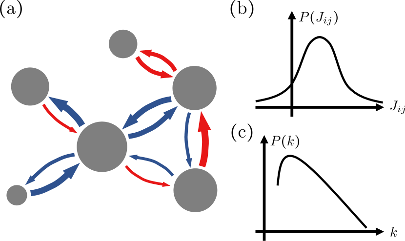
where is the abundance of th species with a self-growth rate , and denotes the summation over all species except . The last term represents the interspecific interaction with two factors: (i) the strength of interaction depicting how much a species affects another species positively or negatively and (ii) the structure of interaction (the adjacency matrix in the context of networks) or indicating the existence or absence of interaction (see Fig. 1 for a graphical illustration). A positive (negative) value of indicates the suppression (promotion) of the growth of by . We set the adjacency matrix to be symmetric, i.e., while we consider and as independent or correlated to some extent controlled by a parameter.
These interspecific interactions, and , do not need to be uniform in nature, and thus we assume the randomness in both and . As in previous studies Bunin (2017); Galla (2018); Roy et al. (2019), for analytic treatment, we set the interaction strength as a Gaussian random variable with the first few moments given by
where . Notations and represent moment and cumulant, respectively, averaged over an ensemble of interaction strength realizations . The sign of represents whether the considered community is overall competitive or cooperative . The characterizes the randomness of interaction strength. The reciprocity is related to the type of pairwise interactions, e.g., with predator-prey interactions .
To represent a heterogeneous interaction structure, we consider an ensemble of adjacency matrices with each element taking and with probability and respectively, and thus satisfying
| (2) |
The number of interacting partners of species is given by called degree and its ensemble average can be heterogeneous if the connection probabilities are not identical.
We use proposed in the static model Goh et al. (2001) to generate networks with the power-law degree distributions , where is the degree exponent, or the Poisson distribution Erdős and Rényi (1959); Gilbert (1959).
We here approximate the connection probability by , which is often called the annealed approximation and valid in uncorrelated networks without a significant degree-degree correlation Newman (2002); Dorogovtsev et al. (2008); Park and Newman (2004).
Under this approximation, the statistical property of is solely determined by the degree sequence , leading to the dynamical equations for the HMFT.
HDMFT.— Using the DMFT technique with the HMFT for Eq. (1) and setting for simplicity, one can obtain the abundance dynamics for a species with degree as follows:
| (3) |
The outcome can be roughly understood by approximating in Eq. (1) as the sum of independent and identically distributed random variables, resulting in along with the Gaussian noise , where and . Here, and are
| (4) | ||||
Equations (3) and (4) are the main results from the HDMFT and their rigorous derivation with moment-generating functional for general is given in Supplemental Material (SM) Sec. I.A. sup . Note that is the average over both species and ensembles of .
The equilibrium abundance follows a truncated Gaussian distribution ,
| (5) |
where is a random variable sampled from the standard Gaussian distribution . Compared with the well-mixed system Bunin (2017); Galla (2018), differences are found in the terms proportional to and in Eq. (5), which bring the degree dependence and fundamental changes to the abundance distribution and survival probability.
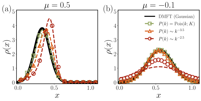
If the degrees of individual species follow a degree distribution , the stationary abundance distribution of the whole community is given by . When all the species have the same degree , i.e., , the truncated Gaussian distribution is recovered, as in fully-interacting systems Bunin (2017); Galla (2018). However, when species exhibit varying degrees, the coalition no longer guarantees a truncated Gaussian distribution for . In Fig. 2, we present obtained with the Poisson distribution and power-law distributions with and , ordered by distribution width (the second cumulant). The DMFT approach extracts only the mean and variance of the overall interactions, including zero components, and approximates as a Gaussian random variable with those mean and variance Barbier et al. (2018). While this method performs well in predicting abundance distributions when degree heterogeneity is relatively small, it fails in cases of large degree heterogeneity. In contrast, our HMDFT method agrees well with simulation results, even with significant degree heterogeneity. Furthermore, our approach accurately describes , distinguishing between species with varying numbers of interacting species, a capability inaccessible to the DMFT method alone (See Sec. II.C. in SM sup ).
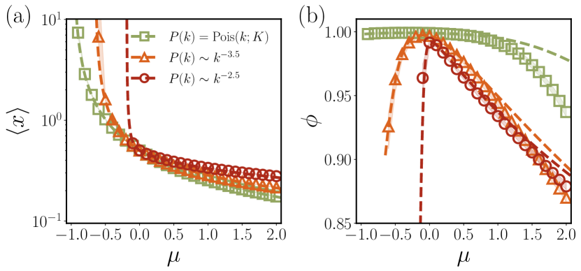
Average abundance and survival probability.—The system-level influence of structural heterogeneity is best manifested in the average abundance and the survival probability with the Heaviside step function . As shown in Fig. 3, for a competitive community , both and decrease monotonically with , i.e., competition curbs the community from growing. On the other hand, in the cooperative community , as gets larger, increases but decreases. It is counterintuitive, as this result indicates that the more species benefit from each other, the more they eventually vanish, whereas the community itself proliferates. This dramatic drop in diversity reflected by is absent in well-mixed systems such as fully-connected case or relatively homogeneous interactions , indicating the important role of interaction structures. Without the explicit consideration of degree heterogeneity, the DMFT alone can never predict this phenomenon.
To excavate the reason behind this seemingly counterintuitive behavior appearing in the cooperative community, let us consider the case with no randomness in strength, . Then all species survive with nonzero abundance , trivially leading to . Thus, cooperative communities are feasible with homogeneous interaction strength by prohibiting survival probability from falling off. Next, let us consider the case without structural heterogeneity, i.e., for all . Then one can find that both and increase with increasing but their ratio remains constant and so does the survival probability , independent of (See Sec. I.C. in SM sup ). For small , we found that is necessary to observe such a diversity drop (See Sec. I.G. in SM sup ). Therefore, without either heterogeneity in strength or structure is there no diversity drop in for .
The counterintuitive drop of diversity with cooperation can be intuitively understood in a star-like network, where numerous “peripheral” species interact with a small number of “hub” species.
The influences of the peripheral species on the hub, when summed up, are likely to be cooperative on average with a small fluctuation due to the central limit theorem.
In contrast, from the viewpoint of peripherical species, the effect from the hub fluctuates under .
Therefore, the hub is very likely to benefit from the peripheral species while hubs could help or suppress the growth of peripheral species by fluctuations.
Moreover, the expectedly large abundance of the hub can threaten a peripheral species even if only a weak competitive interaction is present between them.
This is highly contrasted to the case of no significant heterogeneity in degrees, in which all species, topologically similar, essentially impose an averaged effect on one another with similar abundances.
Abundance and survival of individual species.— Given such difference between hub and peripheral species, we investigate how the fate of individual species is differentiated by their degrees. Using the HDMFT solution in Eq. (5), we calculate the survival probability of a species with degree , represented by a cumulative Gaussian distribution with
| (6) |
The two terms in Eq. (6) represent the self-growth and the expected influences of neighboring species, respectively, as seen in rewriting Eq. (5) as . Each term dominates for and , respectively, with the characteristic degree .
For the competitive case with , species with large may have negative and thereby have small .
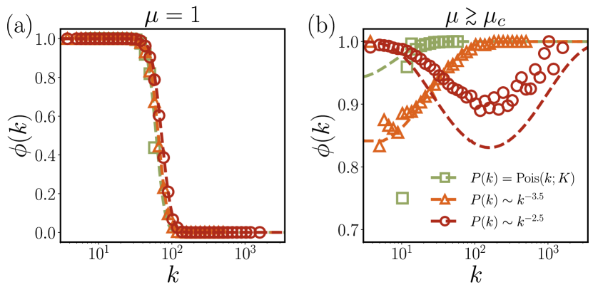
Specifically, the survival probability sharply decreases in the vicinity of [see Fig. 4(a)].
Furthermore, a strong competition drags down, manifested as decreasing with respect to in Fig. 3(a).
On the other hand, for the cooperative case with , becomes positive for all , resulting in .
For the species with as small degree as or as large as , the self-growth or the expected sum of the partners’ influences is likely to dominate the fluctuation of the latter, resulting in large and .
If a species’ degree is comparable to , the fluctuation can be so significant as to make small or zero, reducing and .
We also find that due to decreasing with , low-degree species are more likely to be eliminated under stronger cooperation [see Fig. 4(b)].
Phase diagram.—
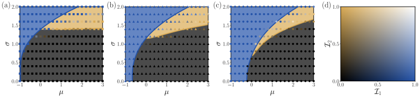
For a comprehensive comparison with previous studies Bunin (2017); Galla (2018), we investigate how the degree heterogeneity affects the phase diagram consisting of the unique fixed point (UFP), unbounded growth (UG), and multiple attractors (MA) phases in the plane by using both numerical solutions to Eq. (1) and the HDMFT prediction.
The results in Fig. 5 first reveal that the UFP phase shrinks as the degree heterogeneity increases.
The triple point is given by from the HDMFT approach, which converges to for with due to the divergence of the second moment (See Sec. I.F. in SM sup ).
Consequently, the system cannot transit directly from the UFP to the UG phase under such strong heterogeneity.
Note that the triple point in Fig. 5(c) does not precisely converge to due to finite-size effects.
Summary and discussion.— We have proposed a novel MF framework capable of addressing two types of heterogeneity in the random Lotka-Volterra systems: the interaction strength with and the interaction structure with . The obtained MF dynamics reveals the differentiation of the individual species’ behaviors depending on their degrees, helping us to understand the presence of the characteristic degree at which the randomness of strength is the most dominant and the origin of nontrivial emergent features of the whole community when both types of heterogeneity are present.
As a final cautionary remark, our approach is based on the moment-generating functional expanded up to the leading order of . The higher-order terms such as and quartic interactions should be considered to study the case of not large enough, the investigation of which will clarify the effects of interaction sparsity. Furthermore, it will allow us to investigate whether our results that degree heterogeneity is a prerequisite for causing diversity drops in cooperative communities still hold for even smaller .
Our framework can be extended in diverse directions, including the incorporation of general distributions of interaction strength, beyond the Gaussian distribution. Another challenging work can be understanding the topological properties of the community of surviving species, including the size and number distributions of the possibly fragmented subcommunities. Finally, we would like to emphasize the broad applicability of our method beyond natural ecosystems, as long as a system is connected by networks and describable through simple equations like GRLV. This includes diverse domains such as economic or political ecosystems, demonstrating the relevance of our theoretical framework across various fields.
Acknowledgements.
This work was supported by the National Research Foundation (NRF) of Korea under Grant Nos. NRF-2021R1C1C1004132 (S.H.L.), NRF-2022R1A4A1030660 (S.H.L.), NRF-2019R1A2C1003486 (D.-S.L.), NRF-RS-2023-00214071 (H.J.P.), and a KIAS Individual Grant(No. CG079902) at Korea Institute for Advanced Study (D.-S.L.) This work was supported by INHA UNIVERSITY Research Grant as well (H.J.P.)References
- Martin et al. (1973) P. C. Martin, E. D. Siggia, and H. A. Rose, Phys. Rev. A 8, 423 (1973).
- Janssen (1976) H.-K. Janssen, Z. Phys. B 23, 377 (1976).
- De Dominicis and Peliti (1978) C. De Dominicis and L. Peliti, Phys. Rev. B 18, 353 (1978).
- Täuber (2014) U. C. Täuber, Critical Dynamics: A Field Theory Approach to Equilibrium and Non-Equilibrium Scaling Behavior (Cambridge University Press, Cambridge, United Kingdom, 2014).
- Crisanti and Sompolinsky (2018) A. Crisanti and H. Sompolinsky, Phys. Rev. E 98, 062120 (2018).
- Sompolinsky et al. (1988) H. Sompolinsky, A. Crisanti, and H.-J. Sommers, Phys. Rev. Lett. 61, 259 (1988).
- Helias and Dahem (2022) M. Helias and D. Dahem, Statistical Field Theory for Neural Networks (Springer, Cham, Switzerland, 2022).
- Mannelli et al. (2020) S. S. Mannelli, G. Biroli, C. Cammarota, F. Krzakala, P. Urbani, and L. Zdeborová, Phys. Rev. X 10, 011057 (2020).
- Poole et al. (2016) B. Poole, S. Lahiri, M. Raghu, J. Sohl-Dickstein, and S. Ganguli, Adv. Neural Inf. Process. Syst. 29 (2016).
- Segadlo et al. (2022) K. Segadlo, B. Epping, A. van Meegen, D. Dahmen, M. Krämer, and M. Helias, J. Stat. Mech. 2022, 103401 (2022).
- Galla and Zhang (2009) T. Galla and Y.-C. Zhang, J. Stat. Mech. 2009, P11012 (2009).
- Baron (2021) J. W. Baron, Phys. Rev. E 104, 044309 (2021).
- Opper and Diederich (1992) M. Opper and S. Diederich, Phys. Rev. Lett. 69, 1616 (1992).
- Sompolinsky and Zippelius (1981) H. Sompolinsky and A. Zippelius, Phys. Rev. Lett. 47, 359 (1981).
- Crisanti et al. (1993) A. Crisanti, H. Horner, and H. J. Sommers, Z. Phys. B 92, 257 (1993).
- Tikhonov and Monasson (2017) M. Tikhonov and R. Monasson, Phys. Rev. Lett. 118, 048103 (2017).
- Yang and Park (2023) S.-G. Yang and H. J. Park, arXiv preprint arXiv:2305.12341 (2023).
- Galla (2018) T. Galla, Europhys. Lett. 123, 48004 (2018).
- Bunin (2017) G. Bunin, Phys. Rev. E 95, 042414 (2017).
- Roy et al. (2019) F. Roy, G. Biroli, G. Bunin, and C. Cammarota, J. Phys. A: Math. Theor. 52, 484001 (2019).
- Biroli et al. (2018) G. Biroli, G. Bunin, and C. Cammarota, New J. Phys. 20, 083051 (2018).
- May (1972) R. M. May, Nature (London) 238, 413 (1972).
- Allesina and Tang (2012) S. Allesina and S. Tang, Nature (London) 483, 205 (2012).
- Baron et al. (2023) J. W. Baron, T. J. Jewell, C. Ryder, and T. Galla, Phys. Rev. Lett. 130, 137401 (2023).
- Jordano et al. (2003) P. Jordano, J. Bascompte, and J. M. Olesen, Ecol. Lett. 6, 69 (2003).
- Krause et al. (2003) A. E. Krause, K. A. Frank, D. M. Mason, R. E. Ulanowicz, and W. W. Taylor, Nature (London) 426, 282 (2003).
- Dunne et al. (2002) J. A. Dunne, R. J. Williams, and N. D. Martinez, Ecol. Lett. 5, 558 (2002).
- Guimarães Jr. (2020) P. R. Guimarães Jr., Annu. Rev. Ecol. Evol. Syst. 51, 433 (2020).
- Montoya and Solé (2002) J. M. Montoya and R. V. Solé, J. Theor. Bio. 214, 405 (2002).
- Newman (2018) M. E. J. Newman, Networks (Oxford University Press, Oxford, United Kingdom, 2018).
- Albert and Barabási (2002) R. Albert and A.-L. Barabási, Rev. Mod. Phys. 74, 47 (2002).
- Barrat et al. (2008) A. Barrat, M. Barthélemy, and A. Vespignani, Dynamical Processes on Complex Networks (Cambridge University Press, Cambridge, United Kingdom, 2008).
- Dorogovtsev et al. (2008) S. N. Dorogovtsev, A. V. Goltsev, and J. F. F. Mendes, Rev. Mod. Phys. 80, 1275 (2008).
- Pastor-Satorras and Vespignani (2001) R. Pastor-Satorras and A. Vespignani, Phys. Rev. E 63, 066117 (2001).
- Kim et al. (2001) B. J. Kim, H. Hong, P. Holme, G. S. Jeon, P. Minnhagen, and M. Y. Choi, Phys. Rev. E 64, 056135 (2001).
- Dorogovtsev et al. (2002) S. N. Dorogovtsev, A. V. Goltsev, and J. F. F. Mendes, Phys. Rev. E 66, 016104 (2002).
- Iglói and Turban (2002) F. Iglói and L. Turban, Phys. Rev. E 66, 036140 (2002).
- Kim et al. (2005) D.-H. Kim, G. J. Rodgers, B. Kahng, and D. Kim, Phys. Rev. E 71, 056115 (2005).
- Lee et al. (2009) S. H. Lee, M. Ha, H. Jeong, J. D. Noh, and H. Park, Phys. Rev. E 80, 051127 (2009).
- Castellano and Pastor-Satorras (2010) C. Castellano and R. Pastor-Satorras, Phys. Rev. Lett. 105, 218701 (2010).
- Costa et al. (2022) G. S. Costa, M. M. de Oliveira, and S. C. Ferreira, Phys. Rev. E 106, 024302 (2022).
- Lee (2005) D.-S. Lee, Phys. Rev. E 72, 026208 (2005).
- Rodrigues et al. (2016) F. A. Rodrigues, T. K. D. Peron, P. Ji, and J. Kurths, Phys. Rep. 610, 1 (2016).
- Barbier et al. (2018) M. Barbier, J.-F. Arnoldi, G. Bunin, and M. Loreau, Proceedings of the National Academy of Sciences 115, 2156 (2018).
- Lee et al. (2022) H. W. Lee, J. W. Lee, and D.-S. Lee, Phys. Rev. E 105, 014309 (2022).
- Marcus et al. (2022) S. Marcus, A. M. Turner, and G. Bunin, PLOS Comput. Biol. 18, e1010274 (2022).
- Poley et al. (2023) L. Poley, J. W. Baron, and T. Galla, Phys. Rev. E 107, 024313 (2023).
- Goh et al. (2001) K.-I. Goh, B. Kahng, and D. Kim, Phys. Rev. Lett. 87, 278701 (2001).
- Erdős and Rényi (1959) P. Erdős and A. Rényi, Publ. Math. Debrecen 6, 290 (1959).
- Gilbert (1959) E. N. Gilbert, Ann. Math. Stat. 30, 1141 (1959).
- Newman (2002) M. E. J. Newman, Phys. Rev. Lett. 89, 208701 (2002).
- Park and Newman (2004) J. Park and M. E. J. Newman, Phys. Rev. E 70, 066117 (2004).
- (53) See Supplemental Materials at [URL].