Incorporating Prior Knowledge of Latent Group Structure in Panel Data Models111Please check here for the latest version.
First Version: June 14, 2022
This Version: August 1, 2025
)
Abstract
The assumption of group heterogeneity has become popular in panel data models. We develop a constrained Bayesian grouped estimator that exploits researchers’ prior beliefs on groups in a form of pairwise constraints, indicating whether a pair of units is likely to belong to a same group or different groups. We propose a prior to incorporate the pairwise constraints with varying degrees of confidence. The whole framework is built on the nonparametric Bayesian method, which implicitly specifies a distribution over the group partitions, and so the posterior analysis takes the uncertainty of the latent group structure into account. Monte Carlo experiments reveal that adding prior knowledge yields more accurate estimates of coefficient and scores predictive gains over alternative estimators. We apply our method to two empirical applications. In a first application to forecasting U.S. CPI inflation, we illustrate that prior knowledge of groups improves density forecasts when the data is not entirely informative. A second application revisits the relationship between a country’s income and its democratic transition; we identify heterogeneous income effects on democracy with five distinct groups over ninety countries.
JEL CLASSIFICATION: C11, C14, C23, E31
KEY WORDS: Grouped Heterogeneity; Bayesian Nonparametrics; Dirichlet Process Prior; Density Forecast; Inflation Rate Forecasting; Democracy and Development.
1 Introduction
Numerous studies have examined and demonstrated the important role of panel data models in empirical research throughout the social and business sciences, as the availability of panel data has increased. Using fixed-effects, panel data permits researchers to model unobserved heterogeneity across individuals, firms, regions, and countries as well as possible structural changes over time. As individual heterogeneity is often empirically relevant, fixed-effects are an objective of interest in numerous empirical studies. For example, teachers’ fixed-effects are viewed as a measure of teacher quality in the literature on teacher valued-added (Rockoff, 2004; Chetty et al., 2014); the heterogeneous coefficients are crucial for panel data forecasting (Liu et al., 2020; Pesaran et al., 2022). In practice, however, researchers may face a short panel where is large and is short and fixed. When applying the least squares estimator for the fixed-effects, a significant number of noisy estimates are produced. To alleviate this issue, a popular and parsimonious assumption that has recently been used is to introduce a group pattern into the individual coefficients, so that units within each group have identical coefficients (Bonhomme and Manresa (2015, BM hereafter), Su et al. (2016), Bonhomme et al. (2022)).
To recover the group pattern, we essentially face a clustering problem, e.g., dividing units into several unknown groups. All existing methods for estimating group heterogeneity solve a clustering problem by assuming that units are exchangeable and treating all units equally a priori. In a cross-country application of evaluating the impact of climate change on economic growth (Hsiang, 2016; Henseler and Schumacher, 2019; Kahn et al., 2021), countries in different climatic zones are assumed to have equal probabilities of being grouped together. The assumption of exchangeability might not be reasonable since correlations are common between observations at proximal locations and researchers could have knowledge of the underlying group structure based on theories or empirical findings. For instance, Sweden and Finland, which share a border, an economic structure, and weather conditions, may have a higher chance of being in the same group than African countries. In such a scenario, it is preferable to use additional information to break the exchangeability between countries to facilitate grouping as opposed to clustering based solely on observations in the sample. The availability of this information drives us to formalize such prior knowledge, which we wish to leverage to improve model performance.
In this paper, we focus on the group heterogeneity in the linear panel data model and develop a nonparametric Bayesian framework to incorporate prior knowledge of groups, which is considered additional information that does not enter the likelihood function. The prior knowledge aids in clustering units into groups and sharpens the inference of group-specific parameters, particularly when units are not well-separated.
The whole framework is built on the nonparametric Bayesian method, where we do not impose a restriction on the number of groups, and model selection is not required. The baseline model is a linear panel data model with an unknown group pattern in fixed-effects, slope coefficients, and cross-sectional error variances. We estimate the model using the stick-breaking representation Sethuraman (1994) of the Dirichlet process (DP) Ferguson (1973, 1974) prior, a standard prior in nonparametric Bayesian inference. In this framework, the number of groups is considered a random variable and is subject to posterior inference. The number of groups and group membership are estimated together with the heterogeneous coefficients. Moreover, since the DP prior implicitly defines a prior distribution on the group partitionings, the posterior analysis takes the uncertainty of the latent group structure into account.
The derivation of the proposed prior starts with summarizing prior knowledge in the form of pairwise constraints, which describe a bilateral relationship between any two units. Inspired by the work of Wagstaff and Cardie (2000), we consider two types of constraints: positive-link and negative-link constraints, representing the preference of assigning two units to the same group or distinct groups. Instead of imposing these constraints dogmatically, each constraint is given a level of accuracy that shows how confident the researchers are in their choice. There is a hyperparameter that controls the overall strength of the prior knowledge: a small value partially recovers the exchangeability assumption on units, whereas a large value confines the prior distribution of group partitioning around group structure based on prior knowledge. We choose the optimal value for the hyperparameter by maximizing the marginal data density. Summarizing prior knowledge in the form of pairwise constraints is practical and flexible since it eliminates the need to predetermine the number of groups and focuses on the bilateral relationships within any subset of units.
The aforementioned pairwise constraints are used to modify the standard DP prior. In particular, the pairwise constraints are combined with the prior distribution of the group partitioning, shrinking the distribution toward my prior knowledge. We refer to the estimator using the proposed prior as the Bayesian group fixed-effects (BGFE) estimator.
We derive a posterior sampling algorithm for the framework with the modified DP prior. Adopting conjugate priors on group-specific coefficients allows for drawing directly from posteriors using a computationally efficient Gibbs sampler. With the newly proposed prior, it can be shown that, compared to the framework that uses a standard DP prior, all that is needed to implement pairwise constraints is a simple modification to the posterior of the group indices.
The pairwise constraint-based framework is closely related and applicable to other models where group structure plays a role. Although we concentrate primarily on the panel data model, the DP prior with pairwise constraints applies to models without the time dimension, such as the standard clustering problem and the estimation of heterogeneous treatment effects. The framework is also applicable to estimating panel VARs (Holland et al., 1983), which involves multiple dependent variables. The group structure is used to overcome overparameterization and overfitting issues by clustering the VAR coefficients into groups, and pairwise constraints add additional information to the highly parameterized model. Moreover, the proposed Gibbs sampler with pairwise constraints is connected to the KMeans-type algorithm, motivating a frequentist’s counterpart of our estimator with a fixed . Essentially, the assignment step in the Pairwise Constrained-KMeans algorithm Basu et al. (2004a), a constrained version of the KMeans algorithm MacQueen et al. (1967), is remarkably similar to the step of drawing a group membership indicator from its posterior. The same exact equivalence can be achieved by applying small-variance asymptotics to the posterior densities under certain conditions. To obtain the frequentist’s analog of our pairwise constrained Bayesian estimators, one can utilize the same approach in BM with the Pairwise Constrained-KMeans algorithm.
We compare the performance of the BGFE estimator to alternative estimators using simulated data. The Monte Carlo simulation demonstrates that the BGFE estimator generates more accurate estimates of the group-specific parameters and the number of groups than the BGFE estimator without including any constraints. The improved performance is mostly attributable to the precise group structure estimation. The BGFE estimator clearly dominates the estimators that omit the group structure by assuming homogeneity or full heterogeneity. We also evaluate the performance of one-step ahead point, set, and density forecasts. Unsurprisingly, the accurate estimates translate into the predictive power of the underlying model; the BGFE estimator outperforms the rest of the estimators.
We apply the proposed method to two empirical applications. An application to forecasting the inflation of the U.S. CPI sub-indices demonstrates that the suggested predictor yields more accurate density predictions. The better forecasting performance is mostly attributable to three key characteristics: the nonparametric Bayesian prior, prior belief on group structure, and grouped cross-sectional heteroskedasticity. In a second application, we revisit the relationship between a country’s income and its democratic transition. This question was originally studied by Acemoglu et al. (2008), who demonstrate that the positive income effect on democracy disappears if country fixed effects are introduced into the model. The proposed framework recovers a group structure with a moderate number of groups. Each group has a clear and distinct path to democracy. In addition, we identify heterogeneous income effects on democracy and, contrary to the initial findings, show that a positive income effect persists in some groups of countries, though quantitatively small.
Literature. This paper relates to the econometric literature on clustering in panel data models. Early contributions include Sun (2005) and Buchinsky et al. (2005). Hahn and Moon (2010) provide economic and theoretical foundations for fixed effects with a finite support. Most recent works focus on linear222See Wang and Su (2021); Bonhomme et al. (2022), among others, for procedures to identify latent group structures in nonlinear panel data models. panel data models with discrete unobserved group heterogeneity. Lin and Ng (2012) and Sarafidis and Weber (2015) apply the KMeans algorithm to identify the unobserved group structure of slope coefficients. Bonhomme and Manresa (2015) also use the KMeans algorithm to recover the group pattern, but they assume group structure in the additive fixed effects. Bonhomme et al. (2022) modify this method and split the procedure into two steps. They first classify individuals into groups using KMeans algorithm and then estimate the coefficients. Ando and Bai (2016) improved on BM’s approach by allowing for group structure among the interactive fixed effects. The underlying factor structure in the interactive fixed effects is the key to forming groups. Su et al. (2016) develop a new variant of Lasso to shrink individual slope coefficients to unknown group-specific coefficients. This method is then extended by Su and Ju (2018) and Su et al. (2019). Freeman and Weidner (2022) consider two-way grouped fixed effects that allow for different group patterns in time and cross-sectional dimensions. Okui and Wang (2021) and Lumsdaine et al. (2022) identify structure breaks in parameters along with grouped patterns. From the Bayesian perspective, Kim and Wang (2019), Zhang (2020), and Liu (2022) adopt the Dirichlet process prior to estimate grouped heterogeneous intercepts in linear panel data models in the semiparametric Bayesian framework. moon2023 incorporate a version of a spike and slab prior to recover one core group of units. Alternative methods, such as binary segmentation (Wang et al., 2018) and assumptions, such as multiple latent groups structure (Cheng et al., 2019; Cytrynbaum, 2021) have also been explored to flourish group heterogeneity literature.
Our work concerns prior knowledge. Bonhomme and Manresa (2015)’s grouped fixed-effects (GFE) estimator is able to include prior knowledge, but it is plagued by practical issues to some extent. They add a collection of individual group probabilities as a penalty term in the objective function, which is a by matrix describing the probability of assigning each unit to all potential groups. This additional penalty term balances the respective weights attached to prior and data information in estimation. The main challenge is providing the set of individual group probabilities for each potential value of as the underlying KMeans algorithm requires model selection. It is rather cumbersome to assess these probabilities for each possible and to adjust for changes in reallocating probabilities across .
None but Aguilar and Boot (2022) explore heterogeneous error variance, and they extend BM’s GFE estimator to allow for group-specific error variances. They modify the objective function to avoid the singularity issue in pseudo-likelihood. Despite the fact that their work paves the way for identifying groups in the error variance, their framework is not yet ready to satisfactorily incorporate prior knowledge because they face the same issue as BM. Building on these works, we investigate the value of prior knowledge of group structure.
This paper also relates to the literature of constraint-based semi-supervised clustering in statistics and computer science. Pairwise constraints have been widely implemented in numerous models and have been shown to improve clustering performance. In the past two decades, various pairwise constrained KMeans algorithms using prior information have been suggested Wagstaff et al. (2001); Basu et al. (2002, 2004a); Bilenko et al. (2004); Davidson and Ravi (2005); Pelleg and Baras (2007); Yoder and Priebe (2017). Prior information is also introduced in the model-based method. Shental et al. (2003) develop a framework to incorporate prior information for the density estimation with Gaussian mixture models. The Dirichlet process mixture model with pairwise constraints has been discussed in Vlachos et al. (2008), Vlachos et al. (2009), Orbanz and Buhmann (2008), Vlachos et al. (2010), Ross and Dy (2013). Lu and Leen (2004), Lu (2007) and Lu and Leen (2007) assume the knowledge on constraints is incomplete and penalize the constraints in accordance with their weights. Law et al. (2004) extents Shental et al. (2003) to allow for soft constraints in the mixture model by adding another layer of latent variables for the group label. Nelson and Cohen (2007) propose a new framework that samples pairwise constraints given a set of probabilities related to the weights of constraints.
Our paper is closely related to Paganin et al. (2021), who address a similar problem using a novel Bayesian framework. Their proposed method shrinks the prior distribution of group partitioning toward a full target group structure, which is an initial clustering of all units provided by experts. This is demanding since not every application can have a full target group structure, as their birth defect epidemiology study did. Our framework circumvents this problem by using pairwise constraints, which are flexibly assigned to any two units. In addition, the induced shrinkage of their framework is produced by the distance function defined by Variation of Information (Meilă, 2007). It can be demonstrated that a partition can readily become caught in local modes, preventing it from ever shrinking toward the prior partition. The use of pairwise relationships in this paper circumvents this issue as well. By fixing the group indices of other pairs, our framework makes sure that the partition with a specific pair that fits our prior belief has a higher prior probability than the partition with a pair that goes against our prior belief.
Outline. In section 2, we present the specification of the dynamic panel data model with group pattern in slope coefficients and error variances and provide details on nonparametric Bayesian priors without prior knowledge, which are then extended to accommodate soft pairwise constraints. Section 3 focuses on the posterior analysis, where the posterior sampling algorithm is provided. We also highlight the posterior estimate of group structure and discuss the connection to constrained KMeans models. We briefly discuss the extensions of the baseline model in section 5. In section 4, we present empirical analysis in which we forecast the inflation rate of the U.S. CPI sub-indices and estimate the country’s income effect on its democracy. Finally, we conclude in section 6. Monte Carlo simulations, additional empirical results, and proofs are relegated to the appendix.
2 Model and Prior Specification
We begin our analysis by setting up a linear panel data model with group heterogeneity in intercepts, slope coefficients, and cross-sectional innovation variance. We then elaborate a nonparametric Bayesian prior for the unknown parameters that takes prior beliefs in the group pattern into account. We briefly highlight several key concepts of a standard nonparametric Bayesian prior as our proposed prior inherits some of its properties.
2.1 A Basic Linear Panel Data Model
We consider a panel with observations for cross-sectional units in periods . Given the panel data set , a basic linear panel data model with grouped heterogeneous slope coefficients and grouped heteroskedasticity takes the following form:
| (2.1) |
where are a vector of covariates, which may contain intercept, lagged , other informative covariates. denote the group-specific slope coefficients (including intercepts). are the group-specific variance. is the latent group index with an unknown number of groups . are the idiosyncratic errors that are independent across and conditional on . They feature zero mean and grouped heteroskedasticity , with cross-sectional homoskedasticity being a special case where . This setting leads to a heterogeneous panel with group pattern modeled through both and .
It is convenient to reformulate the model in (2.1) in matrix form by stacking all observations for unit :
| (2.2) |
where , , , and is a vector of group indices.
Group structure is the key element in our approach. It can be either represented as a vector of group indices describing to which group each unit belongs or as a collection of disjoint blocks induced by , where contains all the units in the -th group and is the number of groups in the sample of size . denotes the cardinality of the set with .
Remark 2.1.
Identification issues may arise with certain specifications. If the grouped fixed-effects in are allowed to vary over time, for example, cannot be identified when the group contains only one unit. Aguilar and Boot (2022) propose a solution, but this problem is beyond the scope of this work. They suggest using the square-root objective function rather than the pseudo-log-likelihood function as the objective function, which replaces the logarithm of with the square root of , to avoid the singularity problem.
Following Sun (2005), Lin and Ng (2012) and BM, we assume that the composition of groups does not change over time. In addition, for any group , we assume that they have different slope coefficients, e.g., , and no single unit can simultaneously belong to these two groups: . Note that these assumptions are used to simplified the prior construction and are not necessary to incorporate prior knowledge. As we show in Section 5, both assumptions can be relaxed by using slightly different priors.
The primary objective of this paper is to estimate the group-specific slope coefficients , group-specific variance , group membership as well as the unknown number of groups using full sample and prior knowledge of the group structure. Given estimates of group-specific coefficients, we are able to offer the point, set, and density forecasts of for each unit . Throughout this paper, we will concentrate on the one-step ahead forecast where . For multiple-step forecasting, the procedure can be extended by iterating in accordance with (2.1) given the estimates of parameters or estimating the model in the style of direct forecasting. The method proposed in this paper is applicable beyond forecasting. In certain applications, the heterogeneous parameters themselves are the objects of interest. For example, the technique developed here can be adapted to infer group-specific heterogeneous treatment effects.
2.2 Nonparametric Bayesian Prior with Knowledge on
We propose a nonparametric Bayesian prior for the unknown parameters with prior beliefs on the group pattern. Figure 1 provides a preview of the procedure for introducing prior knowledge into the model. We propose to use pairwise constraints to summarize researchers’ prior knowledge, with each constraint accompanied by a hyperparameter indicating the researchers’ levels of confidence in their choice. The is then incorporated directly in the prior distribution of the group partition , which is induced from a standard nonparametric Bayesian prior, yielding a new prior. We will elaborate the details throughout this subsection and highlight the clustering properties of the underlying nonparametric Bayesian priors in Section 2.3.
2.2.1 A New Prior with Soft Pairwise Constraints
The derivation of the proposed prior starts from summarizing prior knowledge in the form of pairwise constraints, which describe a bilateral relationship between any two units. Inspired by the literature on semi-supervised learning Wagstaff and Cardie (2000),333We essentially follow the same idea of the pairwise constraints in Wagstaff and Cardie (2000). To better demonstrate the beliefs on constraints, we use different names: positive-link and negative-link, rather than must-link and cannot-link. we consider two types of pairwise constraints: (1) positive-link (PL) constraints, , and (2) negative-link (NL) constraints, . A positive-link constraint specifies that two units are more likely to be assigned to the same group, whereas a negative-link constraint indicates that the units are prone to be assigned to different groups.
Instead of imposing these constraints dogmatically, the constraint between units and is given a hyperparameter which describes how confident the researchers are in their choice for different types of constraints. is continuously valued on the real line, as depicted in Figure 2. On the one hand, the sign of specifies the constraint type, with a positive (negative) value indicating a PL (NL) constraint between and . On the other hand, the absolute value of reflects the strength of the prior belief. We become increasingly confident in our prior belief on units and as . If , we essentially impose the constraint, which is known as a hard PL/NL constraint. Otherwise, it’s a soft PL/NL constraint with a nonzero and finite . if there is no prior belief in units and .
We assume the weight is a logit function of two user-defined hyperparameters444This parametric form is related to the penalized probabilistic clustering proposed by Lu and Leen (2004, 2007). See detailed discussion in Appendix D.2., accuracy and type :
| (2.3) |
Accuracy, , describes the user-specified probability of assigning a constraint for unit and being correct given our prior preference. Specifically, implies the constraint between and must be imposed since we confident that it is accurate, while specifying is equivalent to a random guess or no information is provided. is bounded below by 0.5, following the assumption that leaving the pair unrestricted is more rational than setting a less likely constraint. The type of constraints is denoted by . if unit and are specified to be positive-linked, and for a NL constraints. If the pair doesn’t involve any constraint, we assume .
To incorporate these constraints into the prior, we propose modifying the exchangeable partition probability function (EPPF) or the prior distribution of group indices, , of the baseline Dirichlet process, which we will highlight in the Section 2.3. The resulting group partition will receive a strictly higher (lower) probability if it is (in)consistent with pairwise constraints. As a result, the induced prior on the group indices directly depend on the characteristics of user-specific pairwise constraints and is able to increase or decrease the likelihood of a certain .
In the presence of soft constraints, we modify the EPPF by multiplying a function of characteristics of constraints,
| (2.4) |
where is the prior odds for the constraint between unit and , is a transformed Kronecker delta function such that
| (2.5) |
and is a positive number that controls the overall strength of prior belief. For , corresponds to the baseline EPPF , while for , , where satisfies all pairwise constraints.
Remark 2.2.
Due to the presence of pairwise constraints, the partition probability function presented in (2.4) no longer satisfies the exchangeable assumption as we now distinguish units within each group.
Remark 2.3.
The current framework enables us to impose some constraints. It is an extreme case of soft constraint and thus handy to implement, requiring only setting for the pair . Intuitively, any group partition violating the pairwise constraint between and (i.e., ) will have zero probability, since for such a partition,
and hence the constraint on is imposed and referred to as a hard constraint as opposed to soft constraint. By assigning proper for the pairs , we can flexibly combine soft and hard constraints inside a single specification.
Remark 2.4.
Soft pairwise constraints solve the transitivity issue that might be a problem for hard pairwise constraints. For instance, if we have and , we can still have in the framework of soft pairwise constraints since it preserves the possibility of violating any of these constraints. This is not the case in hard pairwise constraints, as and implies by transitivity.
With the definition of , we rewrite the partition probability function defined in (2.4) in terms of to ease notation,
| (2.6) |
where
| (2.7) |
is a normalization constant and we will use the prior hereinafter. In practice, we will first specify for the constraint between unit and and then construct the corresponding weight via the equation (2.3).
Remark 2.5.
In the particular case where we don’t have any constraint information, reduces to 1 as for all and , and recovers the original DP prior. Hence, our method can cater to all levels of supervision, ranging from hard constraints to a complete lack of constraints.
2.2.2 The Effect of Constraints and Scaling Constant on Group Partitioning
The function in Equation (2.4) is crucial in shifting the prior probability of . By design, when the constraint between and is met in a group partitioning defined by . The prior probability for is therefore increased since . Similarly, if a group partitioning violates the constraint between and , then and the prior probability for drops due to . Therefore, with , the resulting group partition is shrunk toward our prior knowledge without imposing any constraint.
To fix ideas, consider a simplified scenario with units where there are at most two groups. For illustrative purposes, we set the concentration parameter to so that 555Antoniak (1974) provides analytical formulas for probabilities of more general events with larger . In this example, = . if no constraint exists. When , listing all partitions is possible, , and we can calculate the probabilities for each using (2.6). As a result, we are able to derive the probability of units 1 and 2 belonging to the same or different groups, i.e., analytical formulae for and , which neatly demonstrate the effect of and on group partitioning.
It is straightforward to show as a function of , and :
| (2.8) |
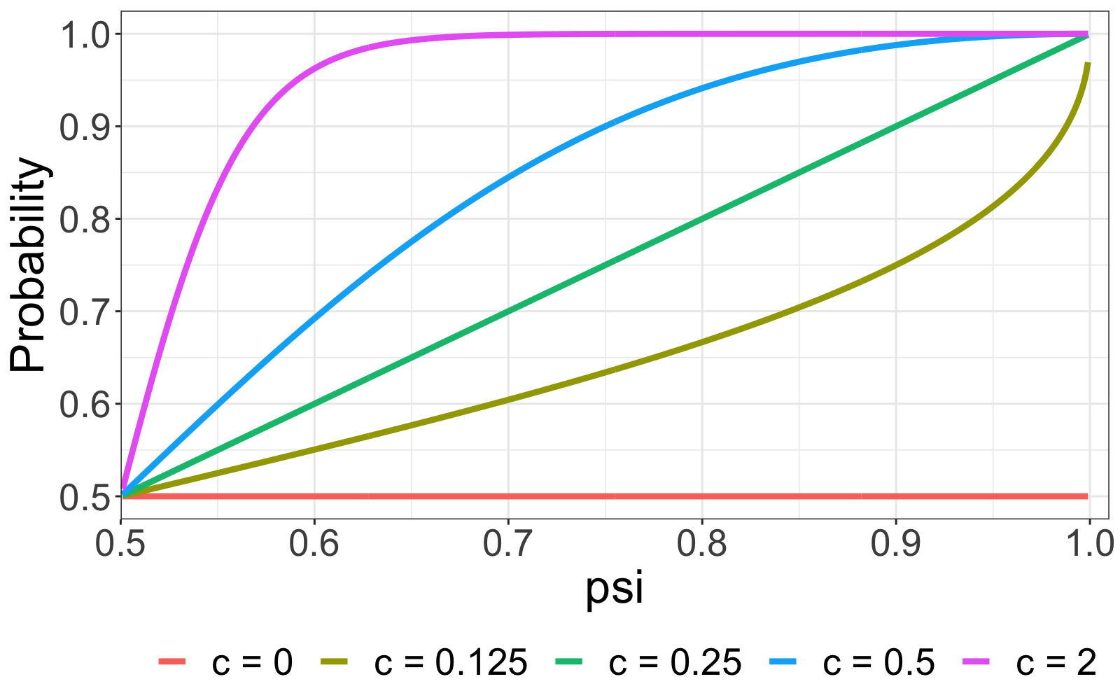
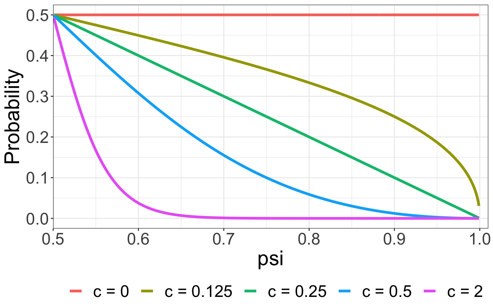
Figure 3 traces out the equation (2.8) for a range of values. The left panel (a) displays the curve for a PL constraint. Firstly, observe that when , remains unchanged at regardless of the value of . This is the situation in which eliminates the constraint’s effect on the prior. Next, given a particular , increases in , which means that a stronger soft PL constraint between units 1 and 2 leads to higher chance of assigning both units to the same group. When is fixed, increasing easily results in a higher , indicating that a larger value magnifies the effect of the PL constraint. In contrast, panel (b) depicts the curve with a NL constraint. and clearly have the opposite effect on : drops significantly as or increases. Notably, even with a large , the soft constraint framework maintains the possibility of breaching the constraint, which is another important feature that preserves the chance of correctly assigning group indices even if the constraint is erroneous.
In the general case where numerous PL and NL constraints are enforced, concurrently affects all constraints. In other words, the value of determines the overall “strength” of the prior belief of . If the prior belief is coherent with the real group partition, it would be preferable to have a large to intensify the effect on constraints, allowing prior information to take precedence over data information, and vice versa.
Remark 2.6.
We propose to find the optimal that maximizes marginal data density using grid search, see details in Appendix 4.1.2. Alternatively, the scaling constant can be pair-specific and data-driven. Basu et al. (2004b), for instance, assume that is a function of observables, i.e., . is monotonically increasing (decreasing) in the distance between units and if they are involved in positive-link (negative-link) constraints. This reflects the belief that if two more distant units are assumed to be positive-linked (negative-linked), their constraint should be given more (less) weight.
2.2.3 Specification of Soft Pairwise Constraints
In reality, it is practical to establish soft pairwise constraints based on existing information on group, even if it is not the genuine group partitioning. In the empirical analysis, for instance, we use the official expenditure categories of CPI sub-indices to construct soft pairwise constraints. When information on group partitioning is insufficient, especially when the number of units is large, these official expenditure categories may serve as a trustworthy starting point. Before formalizing the idea, we first introduce the prior similarity matrix which is a symmetric matrix describing the prior probability of any two units belonging to the same group, i.e., conditional on all hyperparameters in the prior.
The general idea is to derive soft pairwise constraints using the existing information on a preliminary group partitioning , which is allowed to involve only a subset of units. We start with the type of constraints between any two units. Given the preliminary group structure, such as expenditure categories, we specify PL constraints for all pairs of units within the same group and NL constraints for all pairs of units from different groups. This means that we believe the preliminary group structure is correct a priori. Despite the fact that more elaborate and subtle constraints might be implemented, this rough specification is usually a great starting point.
The accuracy for constraints is then specified. When our prior knowledge is limited or the number of units is large, we cannot specify for all pairs with solid knowledge of them. Instead, one desirable yet simple choice is to assume again based on preliminary group partitioning . More specifically, all units in the same group are positive-linked with identical , i.e., for units and from the group , we have . Units from different groups are assumed to be negative-linked with identical , i.e., for units and from distinct groups, we assume and . Following this strategy, depends solely on and hence two units from the same group would have identical soft pairwise constraints with other units. Notice that the number of possible distinct reduces from to , where is the number of groups in and .
This framework permits no prior belief in certain units. If at least one unit in a pair is not included in , we assume that this pair of units is free of constraints and we set to 0 or to 0.5 in the prior. Note that the absence of a constraint does not ensure that the units and are completely unrelated. Instead, if both and are involved in constraints with a third unit , or are connected through a series of constraints, , then the prior probability of and belonging to the same group differs from the prior probability without any constraints. If we wish to prevent two units from linking a priori, they must not be subject to any constraints with the remaining units.
The aforementioned specification strategy induces a block prior similarity matrix, i.e., for an unit , if . Intuitively, if two units have identical soft pairwise constraints and hence posit an identical relationship with all other units, they are equivalent and exchangeable. As a result, these units should have an equal prior probability of sharing the same group index with any other units. More formally,
Theorem 1 (Stochastic Equivalence).
Given two units from the same prior group, if for all , then for all unit in the prior, given weights .
Theorem 1 echos the concept of stochastic equivalence (Nowicki and Snijders, 2001) in stochastic block model666For a more comprehensive review of the stochastic block model, see Lee and Wilkinson (2019). (SBM) (Holland et al., 1983). In less technical terms, for nodes and in the same group, has the same (and independent) probability of connecting with node , as does. Interestingly, this relationship is not coincidental. The prior draw of group membership with the aforementioned specification of and can be viewed as a simulation of a simple SBM. In a simple SBM, there are two essential components: a vector of group memberships and a block matrix, each element of which represents the edge probability of two nodes, given their group memberships. In our case, the preliminary group structure serves as the group membership in SBM. The DP prior and the weight (or and ) of each constraint induce a prior similarity probability comparable to the block matrix.
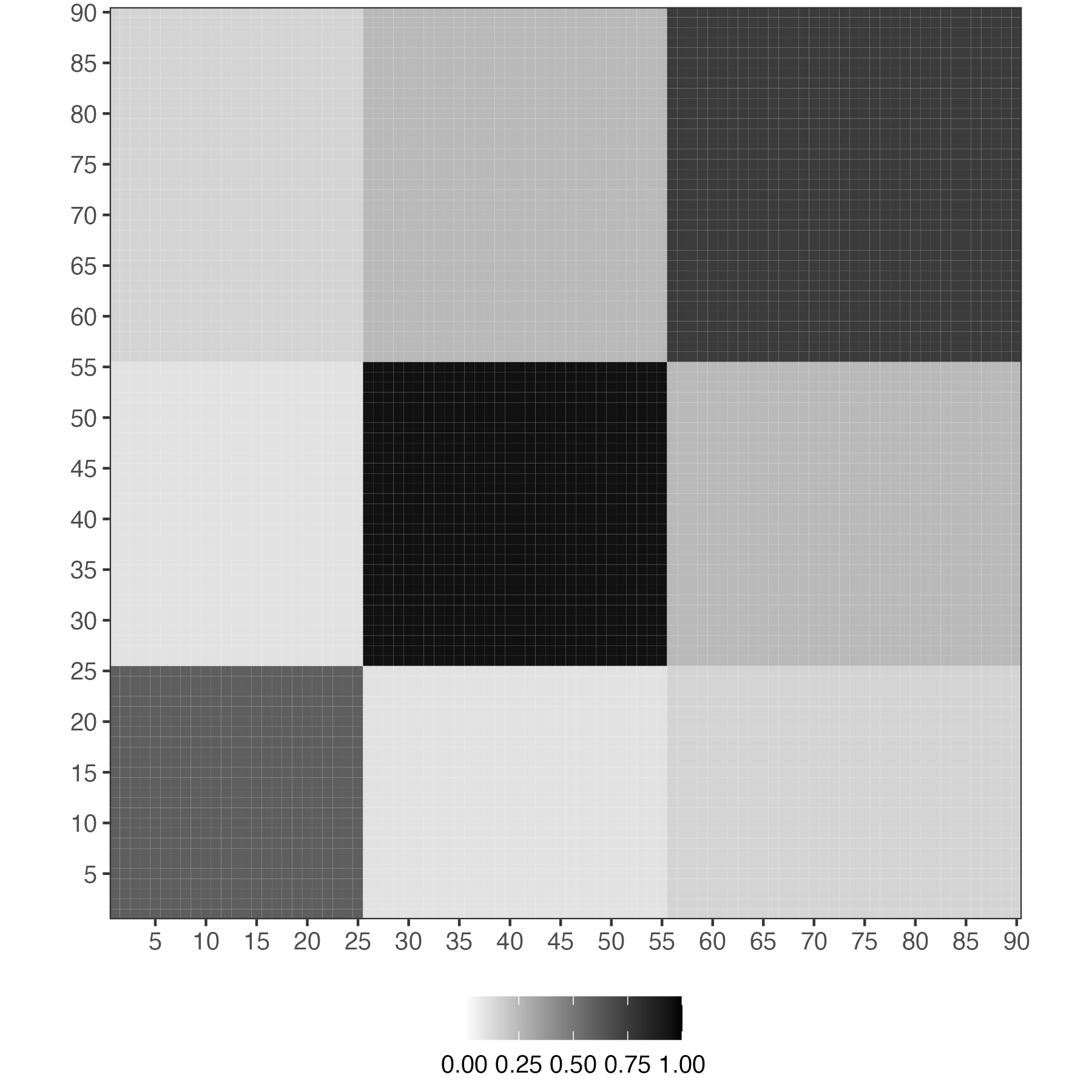
Let’s consider an example of 90 units. The preliminary group structure divides units into 3 groups, with groups 1, 2 and 3 containing 25, 30 and 35 units, respectively. Figure 4 shows the prior similarity matrix, which is based on the aforementioned specification strategy, so it becomes a block matrix with equal entries in each of nine blocks. Units within the same group are stochastically equivalent, as their prior probabilities of being grouped not only with each other but also with units from other groups are the same. As a result, the similarity probability of each pair depends solely on their preliminary membership (and ).
2.2.4 Comparison to Existing Methods
Bonhomme and Manresa (2015) incorporates prior knowledge of group membership by adding a penalty term to the objective function. They assume that prior information is in the form of probabilities which describe the prior probability of unit belonging to group with at most groups as . Consequently, the estimated group index is given by:
| (2.9) |
where is a hyperparameter need to be tuned further and is the predetermined number of groups.
The penalty determines the weights assigned to prior and data information in estimation. Due to the fact that is frequently unknown in advance, this method requires model selection to determine the ideal number of groups. Assume we have alternative options for . We have a matrix for prior information for a given . As a result, in order to pick a model, we must therefore provide sets of prior probability matrix , which is cumbersome and inconvenient. For instance, if has values ranging from and , there are 3,600 entries for , none of which can be missing or undefined. In addition, the information criteria may be unreliable in the finite-sample results, necessitating further care when selecting an appropriate variant for empirical application.
Summarizing prior knowledge through pairwise constraints is often more practical than the penalty function approach in BM and solves the aforementioned practical issues. Pairwise relationships can be derived intuitively from researchers’ input without requiring in-depth knowledge of the underlying groups; researchers do not need to fix the number of groups or group membership a priori. One only needs to focus on a pair of units each time and specify the preference of assigning them to the same or different groups. Moreover, since the pairwise constraints are incorporated into the DP prior, which implicitly defines a prior distribution on the group partitions, model selection is not required and the posterior analysis also takes the uncertainty of the latent group structure into account.
Paganin et al. (2021) offer a statistical framework for including concrete prior knowledge on the partition. Their proposed method aims to shrink the prior distribution towards a complete prior clustering structure, which is an initial clustering involving all units provided by experts. Specifically, they suggest a prior on group partition that is proportional to a baseline EPPF of the DP prior multiplied by a penalization term,
| (2.10) |
with is a penalization parameter, is a suitable distance measuring how far is from , and indicates the same EPPF as in (2.4). Because of the penalization term, the resulting group indices shrink toward the initial target .
This framework is parsimonious and easy to implement, but it comes with a cost. The method is incapable of coping with an initial clustering in a subset of the units under study or multiple plausible prior partitions; otherwise, the distance measure is not well-defined. In addition, the authors suggest utilizing Variation of Information (Meilă, 2007) as the distance measure. It can be shown that the resulting partition can easily become trapped in local modes, leading the partition to never shrink toward . They also argue that other available distance methods have flaws. As a result, the penalty term does not function as anticipated.
Our proposed framework with pairwise constraints is more flexible than adopting a target partition. Actually, the target partition in Paganin et al. (2021) can be viewed as a special case of the pairwise constants, in which every unit must be involved in at least one PL constraint. Our framework could manage partitions involving arbitrary subsets of the units by tactically specifying the bilateral relationships. Most importantly, when the group indices of other pairs are fixed, our framework ensures that the partition containing a specific pair that is consistent with our prior belief receives a strictly greater prior probability than the partition that is inconsistent with our prior belief. This guarantees that the generated shrinks in the direction of our prior belief.
2.3 Nonparametric Bayesian Prior
The baseline model contains the parameters listed below: . We rely mostly on nonparametric Bayesian models.777For a more comprehensive review of the nonparametric Bayesian literature, see Ghosal and Van der Vaart (2017) and Müeller et al. (2018). Bayesian nonparametric models have emerged as rigorous and principled paradigms to bypass the model selection problem in parametric models by introducing a nonparametric prior distribution on the unknown parameters. The prior assumes that a collection of and is drawn from the Dirichlet process prior.888There have been some empirical works that use Dirichlet process model with panel data. Dirichlet process mixture prior is specified for either the distribution of the innovations (Hirano, 2002) or intercepts (Fisher and Jensen, 2022). is a vector of mixture probabilities in Dirichlet process that is produced by the stick-breaking approach with stick length . is the concentration parameter in the Dirichlet process, whereas is a collection of hyperparameters in the base measure . We consider prior distributions in the partially separable form,999The joint prior includes but not . Because the stick-breaking formulation of is a deterministic transformation of , knowing is identical to knowing .
We tentatively focus on the random coefficients model where, conditional on , and are independent to the conditional set that includes initial value of each unit , the initial values of predetermined variables, and the whole history of exogenous variables. The assumption guarantees that and can be sampled separately and simplifies the inference of the underlying distribution of and to an unconditional density estimation problem, therefore lowering computational complexity. The joint distribution of heterogeneous parameters as a function of the conditioning variables can then be modeled to extend the model to the correlated random coefficient model, which is briefed in Section 2.3.3. A full explanation and derivation for the correlated random coefficient model are provided in the online appendix.
2.3.1 Prior on Group-Specific Parameters
In the nonparametric Bayesian literature, the Dirichlet Process (DP) prior Ferguson (1973, 1974); Sethuraman (1994) is a canonical choice, notable for its capacity to construct group structure and accommodate an infinite number of possible group components.101010See Appendix A.1 for a brief overview of the DP and Appendix A.1.3 for its clustering properties. The DP mixture is also known as a “infinite” mixture model due to the fact that the data indicate a finite number of components, but fresh data can uncover previously undetected components Neal (2000). When the model is estimated, it chooses automatically an appropriate subset of groups to characterize any finite data set. Therefore, there is no need to determine the “proper” number of groups.
The DP prior can be written as an infinite mixture of point mass with the probability mass function:
| (2.11) |
where denotes the Dirac-delta function concentrated at and is the base distribution. We adopt an Independent Normal Inverse-Gamma (INIG) distribution for the base distribution :
| (2.12) |
with a set of hyperparameters .
The group probabilities are constructed by an infinite-dimensional stick-breaking process Sethuraman (1994) governed by the concentration parameter ,
| (2.13) |
where stick lengths are independent random variables drawn from the beta distribution,111111Recall that a distribution is supported on the unit interval and has mean . . The group probability will be random but still satisfy almost surely.
Equation (2.13) is essential to understanding how the DP prior controls the number of groups. The building of group probabilities is compared to the breaking of a stick of unit length sequentially, in which the length of each break is assigned to the current value of . As the number of groups increases, the probability created by the stochastic process decreases because the remaining stick becomes shorter with each break. In practice, the number of groups does not increase as fast as due to the characteristic of the stick-breaking process that leads the group probability to soon approach zero.
Although in principle we do not restrict the maximum number of groups and allow the number to rise as increases, a finite number of instances will only occupy a finite number of components. The concentration parameter in the prior of determines the degree of discretization – the complexity of the mixture and, consequently, , as also revealed in (A.3). As , the realizations are all concentrated at a single value, however as , the realizations become continuous-valued as its based distribution. Specifically, Antoniak (1974) derives the relationship between and the number of unique groups,
that is, the expected number of unique groups is increasing in both and the number of units .
Escobar and West (1995) highlights the importance of specifying when imposing prior smoothness on an unknown density and demonstrates that the number of estimated groups under a DP prior is sensitive to . This suggests that a data-driven estimate of is more reasonable. Moreover, Ascolani et al. (2022) emphasizes the importance of introducing a prior for as it is crucial for learning the true number of groups as increases and hence establishing the posterior consistency. We define a gamma hyperprior for and update it based on the observed data in order to alter the smoothness level. This step generates a posterior estimate of , which indirectly determines the number of groups without reestimating the models with different group sizes. Essentially, this represents “automated” model selection.
Collectively, we specify a DP prior for . The DP prior is a mixture of an infinite number of possible point masses, which can be constructed through the stick-breaking process. The discretization of the underlying distribution is governed by the concentration parameter . With a hyerprior on , we permit the data to determine the number of groups present in the data, which can expand unboundedly along with the data.
2.3.2 Prior on Group Partitions
In a formal Bayesian formulation, a prior distribution is specified to partition with associated indices . Despite the fact that DP prior does not specify this prior distribution explicitly, we can characterize it using the exchangeable partition probability function (EPPF) (Pitman, 1995). As we briefly mentioned in the last subsection, the EPPF plays a significant role in connecting the prior belief on group structure to the DP prior, which is included as part of our proposed prior distribution in Equation (2.4).
The EPPF characterizes the distribution of a partition induced by . As the generic Dirichlet process assumes units are exchangeable, any permutation has no effect on the joint probability distribution of ; hence, the EPPF is determined entirely by the number of groups and the size of each group. Pitman (1995) demonstrates that the EPPF of the Dirichlet process has the closed form,
| (2.14) |
where is the concentration parameter and denotes the Gamma function. Note that the partition is conceived as a random object and hence the group number is not predetermined, but rather is a function of , .
Sethuraman (1994) and Pitman (1996) constructively show that group indices/partitions can be drawn from the EPPF for DP using the stick-breaking process defined in (2.13). As a result, the EPPF does not explicitly appear in the posterior analysis in the current setting so long as the priors for the stick lengths are included.
2.3.3 Correlated Random Coefficients Model
As suggested by Chamberlain (1980), allowing the individual effects to be correlated with the initial condition can eliminate the omitted variable bias. This subsection presents the first attempt to introduce dependence between grouped effects and covariates, under the presence of group structure in both heterogeneous slope coefficients and cross-sectional variance. The underlying theorems, such as posterior consistency, and the performance of the framework are left for future study.
We primarily follow the proposed framework in Liu (2022) and utilize Mixtures of Gaussian Linear Regressions (MGLRx) for the group-specific parameters. MGLRx prior is discussed in Pati et al. (2013) and can be viewed as a Dirichlet Process Mixture (DPM) prior that takes the dependence of covariates into account. Notice that the correlated random coefficients model requires a DPM-type prior for and . This is because and are assumed to be correlated with covariates of each individual, and as such, they are not identical within a group.
Following Liu (2022), we first transform and define , where is some small (large) positive number. This transformation simplifies the prior for , which is now dependent on covariates, and ensures that a similar prior structures can be applied to both and .
In the correlated random coefficients model, the DPM prior for or is an infinite mixture of Normal densities with the probability density function:
| (2.15) | |||
| (2.16) |
where is the conditioning set at period 0, which includes initial value of each unit , the initial values of predetermined variables, and the whole history of exogenous variables. Notice that and share the same set of group probabilities .
Similar but not identical to the DP prior, it is the component parameters or that are directly drawn from the base distribution . is assumed to be a conjugate Matricvariate-Normal-Inverse-Wishart distribution.
The group probabilities are now characterized by a probit stick-breaking process (Rodriguez and Dunson, 2011),
| (2.17) |
where the stochastic function is drawn from a Gaussian process, for . The Gaussian process is assumed to have zero mean and the covariance function . defined as follows,
| (2.18) |
where and has its own hyperprior, see details in Pati et al. (2013).
3 Posterior Analysis
This section describes the procedure for analyzing posterior distributions for the baseline model described in (2.1) with the priors specified in Section 2.2.1. The joint posterior distribution of model parameters is
| (3.1) |
where is the likelihood function given by equation (2.1) for an i.i.d. model conditional on group indices , and is the additional term of pairwise constraints with the form .
3.1 Posterior Sampling
Draws from the joint posterior distribution can be obtained by using blocked Gibbs sampling. The algorithm is derived from Ishwaran and James (2001) and Walker (2007). Due to the use of a finite-dimensional prior and truncation, the method described in Ishwaran and James (2001) cannot truly address our demand for estimating the number of groups without a predetermined value or upper bound. We employ the slice sampler (Walker, 2007), which is the exact block Gibbs sampler for the posterior computation in infinite-dimensional Dirichlet process models, modifying the block Gibbs sampler of Ishwaran and James (2001) to avoid truncation approximations. Walker (2007) augments the posterior distribution with a set of auxiliary variables consisting of i.i.d. standard uniform random variables, i.e., for . The augmented posterior is then represented as
| (3.2) |
where is substituted for in the equation (3).
To roughly see how slice sampling works, recall that the group probabilities are constructed in a sequential manner, following a stick-breaking procedure. The leftover of the stick after each break gets smaller and smaller. Given the finite number of units, we can always find the smallest such that for all groups , the minimum of among all units is larger than , which is bounded above by the length of the leftover after breaks, . More formally,
| (3.3) |
As a result, all units receive strictly zero probability of being assigned to any group since the indicator function is zero.
There are two advantages to incorporating the auxiliary variable into the model. First and foremost, directly determines the largest possible number of groups in each sampling iteration. This reduces the support of and to a finite space, enabling us to solve a problem of finite dimensions without truncation. Furthermore, have no effect on the joint posterior of other parameters because the original posterior can be restored by integrating out for .
The Gibbs sampler are used to simulate the joint posterior distribution of . We break this vector into blocks and sequentially sampling for each block conditional on the current draws for the other parameters and the data. The full conditional distributions for each block are easily derived using the conjugate priors specified in Section 2.
For the group-specific parameters, we directly draw samples from their posterior densities as we adapt conjugate priors. The posterior inference with respect to becomes standard once we condition on the latent group indices . It is essentially a Bayesian panel data regression for each group. The conditional posterior for the stick length is a beta distribution given , and hence direct sampling is possible.
We follow Walker (2007) to derive the posterior of auxiliary variable . As are standard uniformly distributed, the posterior is a uniform distribution defined on , conditional on the group probabilities and group indices. In terms of the concentration parameter , we use a 2-step procedure proposed by Escobar and West (1995). Following their approach, we first draw a latent variable from . Then, given and number of groups in the current iteration, we directly draw from a mixture of two Gamma distribution.
It is worth noting that the steps for implementing the DP prior with or without soft pairwise constraints are the same for all parameter besides the group indices . This is due to the fact that soft pairwise constraints only affect other parameters through the group indices. It is handy to sample group indices with soft pairwise constraints conditional on other parameters. The posterior probability of assigning unit to group includes additional term to rewards (penalizes) the abidance (violation) of constraints,
| (3.4) |
where is the maximal number of groups after generating potential new group-specific slope coefficients and variance. We then draw the group index for unit from a multinomial distribution:
| (3.5) |
Algorithm 1 below summarizes the algorithm for the proposed Gibbs sampling. For illustrative purposes, we focus primarily on the posterior densities of major parameters and omit details on step (vii). In short, step (vii) creates potential groups by sampling new from the prior if the latest based on newly drawn and is larger than previous , which indicate the current iteration permits more groups. This Detailed derivations and explanation of each step are provided in Appendix C.2.
Algorithm 1.
(Gibbs Sampler for Random Coefficients Model with Soft Pairwise Constraints)
For each iteration ,
-
(i)
Calculate number of active groups:
-
(ii)
Group-specific slope coefficients: draw from for .
-
(iii)
Group-specific variance: draw from for .
-
(iv)
Group “stick length”: draw from for and update group probability in accordance to the stick-breaking procedure.
-
(v)
Auxiliary variable: draw from for and calculate .
-
(vi)
DP concentration parameter: draw a latent variable from and draw from .
-
(vii)
Generate potential groups based on and find the maximal number of groups .
-
(xi)
Group indices: draw from for and .
3.2 Determining Partition
In contrast to popular algorithms such as agglomerative hierarchical clustering or the KMeans algorithm, which return a single clustering solution, Bayesian nonparametric models provide a posterior over the entire space of partitions, enabling the assessment of statistical properties, such as the uncertainty on the number of groups.
However, when the group structure is part of the major conclusion of an empirical analysis, the point estimate of group structure becomes crucial. Wade and Ghahramani (2018) discuss in detail an appropriate point estimate of the group partitioning based on the posterior draws. From the decision theory, the point estimate minimizes the posterior expected loss,
where the loss function is the variation of information by Meilă (2007), which measures the amount of information lost and gained in changing from partition to .121212Another possible loss function is the 0-1 loss function , which leads to being the posterior mode. This loss function is undesirable since it ignores similarity between two partitions. For instance, a partition that deviates from the truth in the allocation of only one unit is penalized the same as a partition that deviates from the truth in the allocation of numerous units. Furthermore, it is generally recognized that the mode may not accurately reflect the distribution’s center. The Variation of Information is based on the Shannon entropy , and can be computed as
where denotes base 2, is the cardinality of the group , and the size of blocks of the intersection and hence the number of indices in block under partition and block under .
3.3 Connection to Constrained KMeans Algorithm
The procedure of Gibbs sampling with soft constraints in Algorithm 1 is closely related to constrained clustering in the computer science literature. In this parallel literature, constrained clustering refers to the process of introducing prior knowledge to guide a clustering algorithm. For a subset of the data, the prior knowledge takes the form of constraints that supplement the information derived from the data via a distance metric. As we shall see below, under several simplifying assumptions, our framework could be reduced to a deterministic method for estimating group heterogeneity using a constrained KMeans algorithm. Though this deterministic method may address the practical issues in BM, it only works for certain restricted models and hence is not as general as our proposed framework.
We start with a brief review of the Pairwise Constrained KMeans (PC-KMeans) clustering algorithm by Basu et al. (2004a), which is a well-known clustering algorithm in the field of semi-supervised machine learning. It’s a pairwise constrained variant of the standard KMeans algorithm in which an augmented objective function is used in the assignment step. Given a collection of observations , a set of positive-link constraints , a set of negative-link constraints , the cost of violating constraints and the number of groups , the PC-KMeans algorithm divides observations into groups (the assignment step) so as to minimize the following objective function,
| (3.7) |
where is the centroid of group , i.e., , is the set of units assigned to group , and is the size of group . The first part is the objective function for the conventional KMeans algorithm, while the second part accounts for the incurred cost of violating either PL constraints () or NL constraints ().
Similar to KMeans, PC-KMeans alternates between reassigning units to groups and recomputing the means. In the assignment step, it determines a disjoint partitioning that minimizes (3.7). Then the update step of the algorithm recalculates centroids of observations assigned to each cluster and updates for all .
By applying asymptotics to the variance of distributions within the model, we demonstrate linkages between the posterior sampler of our constrained BGFE estimator and KMeans-type algorithms in Theorem 2. We investigate small-variance asymptotics for posterior densities, motivated by the asymptotic connection between the Gibbs sampling algorithm for the Dirichlet process mixture model and KMeans Kulis and Jordan (2011), and demonstrate that the Gibbs sampling algorithm for the CBG estimator with soft constraints encompasses the constrained clustering algorithm PC-KMean in the limit.
Theorem 2.
(Equivalency between BGFE with Soft Constraints and PC-KMeans)
If the following conditions hold,
-
(i)
group pattern is in fixed-effects but not in slope coefficients, i.e., . Other covariates might be introduced, but they cannot have grouped effects on ;
-
(ii)
The number of group is fixed at ;
-
(iii)
Homoscedasticity: for all ;
-
(iv)
Constraint weights is scaled by the variance of errors: ;
then the proposed Gibbs sampling algorithm for the BGFE estimator with soft constraint embodies the PC-KMeans clustering algorithm in the limit as . In particular, the posterior draw of group indices is the solution to the PC-KMeans algorithm.
We return to the world of grouped fixed-effects models. In fact, the clustering algorithm is essential for BM and Bonhomme et al. (2022), who use the KMeans algorithm to reveal the group pattern in the fixed-effects. With the theorem described above, it motivates a constrained version of BM’s GFE estimator. We show that it is straightforward to incorporate prior knowledge in the form of soft paired restrictions into the GFE estimator. The soft pairwise constrained grouped fixed-effects (SPC-GFE) estimator is defined as the solution to the following minimization problem given the number of groups :
| (3.8) |
where the minimum is taken over all possible partitions of the units into groups, common parameters , and group-specific time effects . and are the user-specified costs on PL and NL constraints.
For given values of and , the optimal group assignment for each individual unit is
| (3.9) |
where we essentially apply the PC-KMeans algorithm to get the group partition. The SPC-GFE estimator of in (3.8) can then be written as
| (3.10) |
where is given by (3.9). and are computed using an OLS regression that controls for interactions of group indices and time dummies. The SPC-GFE estimate of is then simply .
Remark 3.1.
While the SPC-GFE estimator implements soft constraints, it still requires a predetermined number of group and model selection.
4 Empirical Applications
We apply our panel forecasting methods to the following two empirical applications: inflation of the U.S. CPI sub-indices and the income effect on democracy. The first application focuses mostly on predictive performance, whereas the second application focuses primarily on parameter estimation and group structure.
4.1 Model Estimation and Measures of Forecasting Performance
To accommodate richer assumptions on model, we use variants of the baseline model in Equation (2.1) in this section, either by adding common regressors or allowing for time-variation in the intercept. We use the conjugate prior for all parameters, see details in Appendix B.
4.1.1 Specification of Constraints
In both applications, the prior knowledge of the latent group structure or the pre-grouping structure covers all units. In the first application, CPI sub-indices can be clustered by expenditure category, whereas countries in the second application may be grouped according to their geographic regions. We build positive-link and negative-link constraints given the prior knowledge: all units within the same group are presumed to be positive-linked, while units from different categories are believed to be negative-linked. In terms of the accuracy of constraints, and are equal for all constraints with the same type, following the strategy described in Section 2.2.3. In the applications below, we fix and to reflect the belief that PL constraints (attracting forces) play slightly more important role than the NL constraints (repelling forces) and NL constraints cannot be ignored. Finally, we construct weights using (2.3). Notice that these assumptions on prior and hyperparameters are an example to showcase how the proposed framework works with real data. In practice, we may specify constraints for a subset of units with different levels of weights, either in a data-driven manner (for instance, highly correlated units may fall into the same group with a high level of confidence) or in a model-based manner (i.e., is a function of covariates).
4.1.2 Determining the Scaling Constant
Given that the dimension of the space of group partitions increases exponentially with the number of units , attention must be given while selecting across analyses with different . As suggested by Paganin et al. (2021), calibrating the modified prior is computationally intensive. We are facing a trade-off between investing time to get the prior “exactly right” and letting the constant be an estimated model parameter. As such, we propose to find the optimal that maximizes marginal data density using grid search.
In the Monte Carlo simulation, the value of is fixed for simplicity, but in the empirical applications, is determined by marginal data density (MDD). We calculate MDD using the harmonic mean estimator (Newton and Raftery, 1994), which defined as
| (4.1) |
given a sample from the posterior . The simplicity of the harmonic mean estimator is its main advantage over other more specialized techniques. It uses only within-model posterior samples and likelihood evaluations, which are often available anyway as part of posterior sampling. We finally choose the optimal value for that maximizes MDD.
4.1.3 Estimators
We consider six estimators in the section. The first three estimators are our proposed Bayesian grouped fixed-effects (BGFE) estimator with different assumptions on cross-sectional variance and pairwise constraints. The last three estimator ignore the group structure.
-
(i)
BGFE-he-cstr: group-specific slope coefficients and heteroskedasticity with constraints.
-
(ii)
BGFE-he: group-specific slope coefficients and heteroskedasticity without constraints.
-
(iii)
BGFE-ho: homoskedastic version of BGFE-he.
-
(iv)
Pooled OLS: fully homogeneous estimator
-
(v)
AR-he: flat-prior estimator that assumes corresponds to standard AR model with additional regressor in this environment.
-
(vi)
AR-he-PC: AR-he with the lagged value of the first principal component as additional regressor.
In the first application, we focus on inflation forecasting. For the most recent advances in this topic, Faust and Wright (2013) provide a comprehensive overview of a large set of traditional and recently developed forecasting methods. Among many candidate methods, we choose the AR model as the benchmark and exclusively include it as an alternative estimator in this exercise. This is because the AR is relatively hard to beat and, notably, other popular methods, such as the Atkeson–Ohanian version random walk model (Atkeson et al., 2001), UCSV (Stock and Watson, 2007), and TVP-VAR (Primiceri, 2005), generally do as reasonably well as the AR model, according to Faust and Wright (2013).
4.1.4 Posterior Predictive Densities
We generate one-step ahead forecasts of for conditional on the history of observations
and newly available variables at .
The posterior predictive distribution for unit is given by
| (4.2) |
where is a vector of parameters . This density is the posterior expectation of the following function:
| (4.3) |
which is invariant to relabeling the components of the mixture and is the number of groups in . Given posterior draws, the posterior predictive distribution estimated from the MCMC draws is
| (4.4) |
where
| (4.5) |
We can therefore draw samples from by simulating (2.1) forward conditional on the posterior draws of and observations. Note that MCMC exhibits the true Bayesian predictive distribution, implicitly integrating over the entire underlying parameter space.
4.1.5 Point Forecasts
We evaluate the point forecasts via the real-time recursive out-of-sample Root Mean Squared Forecast Error (RMSFE) under the quadratic compound loss function averaged across units. Let represent the predicted value conditional on the observed data up to period , the loss function is written as
| (4.6) |
where is the realization at and denote the forecast error.
The optimal posterior forecast under quadratic loss function is obtain by minimizing the posterior risk,
| (4.7) |
This implies optimal posterior forecast is the posterior mean,
| (4.8) |
Conditional on posterior draws of parameters, the mean forecast can be approximated by the Monte Carlo averaging,
| (4.9) |
Finally, the RMSFE across units is given by
| (4.10) |
4.1.6 Density Forecasts
To compare the performance of density forecasts for various estimators, we report the average log predictive scores (LPS) to assess the performance of the density forecast from the view of the probability distribution function. As suggested in Geweke and Amisano (2010), the LPS for a panel reads as,
| (4.11) |
where the expectation can be approximated using posterior draws:
| (4.12) |
4.2 Inflation of the U.S. CPI Sub-Indices
Policymakers and market participants are very interested in the abilities to reliably predict the future disaggregated inflation rate. Central banks predict future inflation trends to justify interest rate decisions, control and maintain inflation around their targets. The Federal Reserve Board forecasts disaggregated price categories for short-term inflation forecasting (Bernanke, 2007). They rely primarily on the bottom-up approach that focuses on estimating and forecasting price behavior for the various categories of goods and services that make up the aggregate price index. Moreover, investors in fixed-income markets in the private sector wish to forecast future sectoral inflation in order to anticipate future trends in discounted real returns. Some private firms also need to predict specific inflation components in order to forecast price dynamics and reduce risks accordingly.
In this section, we demonstrate the use of constrained BGFE estimators with prior knowledge on the group pattern to forecast inflation rates for the sub-indices of U.S. Consumer Expenditure Index (CPI). We focus primarily on the one-step ahead point and density forecast. Due to space constraints, we only report the group partitioning for the most recent month in the main text.
4.2.1 Model Specification and Data
Model: We start by exploring the out-of-sample forecast performance of a simple, generic Phillips curve model. It is a panel autoregressive distributed lag (ADL) model with a group pattern in the intercept, coefficients, as well as error variance. The model is given by
| (4.13) |
where is year-over-year inflation rate, i.e., , and is the slack measure for the labor market, the unemployment gap. We fix at 3 because the benchmark AR model would have the best predictive performance.
Data: We collect the sub-indices of CPI for all urban consumer (CPI-U) that include food and energy. The raw data is obtained from the U.S. Bureau of Labor Statistics (BLS), which is recorded on a monthly basis from January 1947 to August 2022. The CPI-U is a hierarchical composite index system that partitions all consumer goods and services into a hierarchy of increasingly detailed categories. It consists of eight major expenditure categories (1) Apparel; (2) Education and Communication; (3) Food and Beverages; (4) Housing; (5) Medical Care; (6) Recreation; (7) Transportation; (8) Other Goods and Services. Each category is composed of finer and finer sub-indexes until the most detailed levels or “leaves” are reached. This hierarchical structure can be represented as a tree structure, as shown in Figure 5. It is important to note that the parent series and its child series may be highly correlated and readily form a group due to the fact that parent series are generated from child series. For instance, the Energy Services is expected to correlated with its child series Utility gas service and Electricity. Due to our focus on group structure, it is vital to eliminate all parent series in order to prevent not just double-counting but also dubious grouping results. More details regarding the data are provided in Appendix F.1.
forked edges, for tree= grow = east, align = left, font=, [All Items [Housing [Shelter [Rent of primary residence] [Owners’ equivalent rent of residences] ] [Fuels and utilities [Water sewer and trash] [Household energy [Fuel oil and other fuels [Fuel oil] [Propane kerosene and firewood]] [Energy services [Electricity] [Utility gas service]]] ] ] [Transportation […] ] [Food and beverages […] ] ]
Pre-grouping: The official expenditure categories are used to build PL and NL constraints: all units within the same categories are presumed to be positive-linked, while units from different categories are believed to be negative-linked.
We focus on the CPI sub-indices after January 1990 for two reasons: (1) the number of sub-indices before 1990 was relatively small, diminishing the importance of the group structure; and (2) the consumption has been changed and more expenditure series were introduced in the 1990s as a result of the popularity of electronic products, food care, etc. After the elimination of all parent nodes, the unbalanced panel consists of 156 sub-indices in eight major expenditure categories. We employ rolling estimation windows of 48 months131313The benchmark AR-he model scores the best overall performance with a window size of 48. and require each estimation sample to be balanced, removing individual series lacking a complete set of observations in a given window. Finally, we generate 329 samples with the first forecast produced for April 1995.
4.2.2 Results
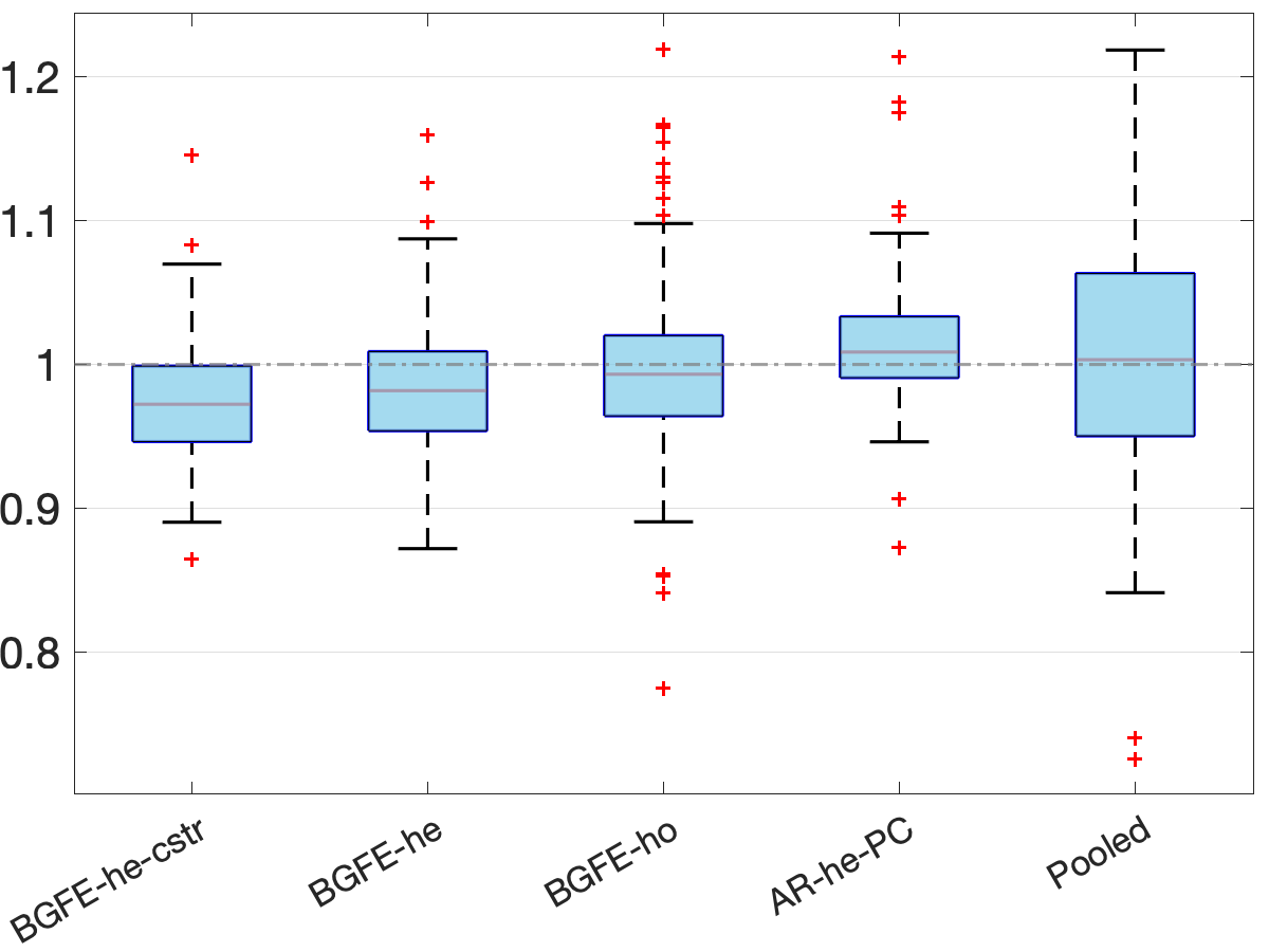
We begin the empirical analysis by comparing the performance of point and density forecasts across 329 samples. Throughout the analysis, the AR-he estimator serves as the benchmark as it essentially assumes individual effects.
In Figure 6, we present the frequency of each estimator with the lowest RMSFE in the panel (a) and the boxplot141414The boundaries of the whiskers is based on the 1.5 IQR value. All other points outside the boundary of the whiskers are plotted as outliers in red crosses. of the ratio of RMSFE relative to the AR-he estimator in the panel (b). First, the AR-he and AR-he-PC estimators, which rely only on an individual’s own past data, are not competitive in point forecasts and perform considerably worse than the others. This implies that it is highly advantageous to explore cross-sectional information to improve point forecasts. Moreover, the BGRE-he-cstr estimator scores the highest frequency of being the best estimator despite the fact that BGFE-he-cstr, BGFE-he, BGFE-ho, and pooled OLS estimators all utilize cross-sectional information. Examining the box plot, we find that the BGFE-ho and pooled OLS estimators, which overlook heteroskedasticity, can achieve greater performance in some samples, but make poorer forecasts more often than the other estimators. BGFE-he-cstr and BGFE-he estimator, on the other hand, typically outperform the others and the benchmark in terms of median RMSFE and the ability to produce forecasts with the lowest RMSFE without also increasing the risk of generating the least accurate forecasts.
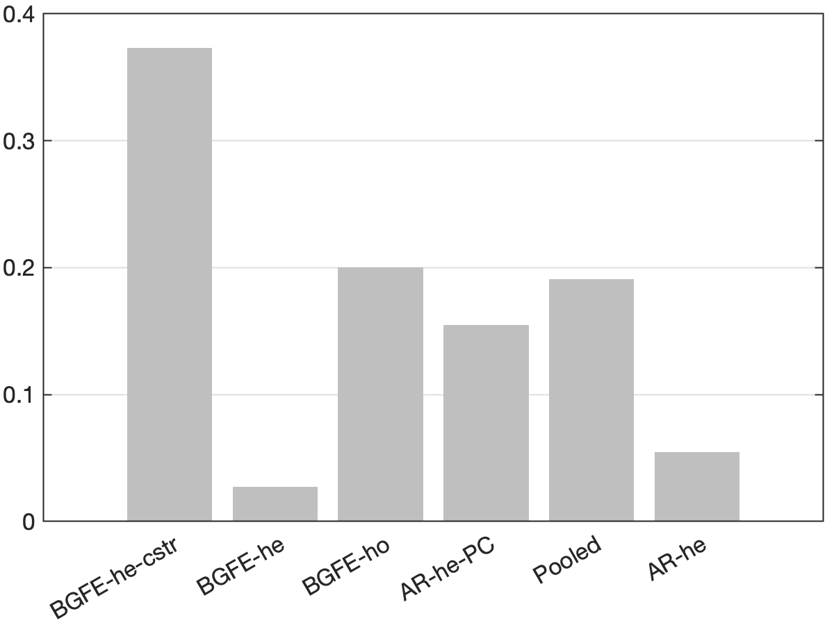
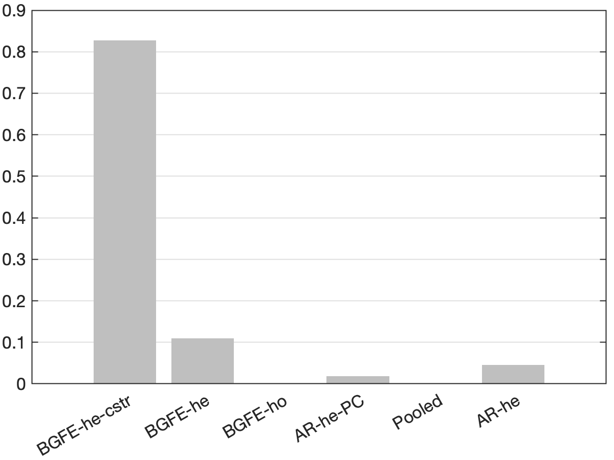
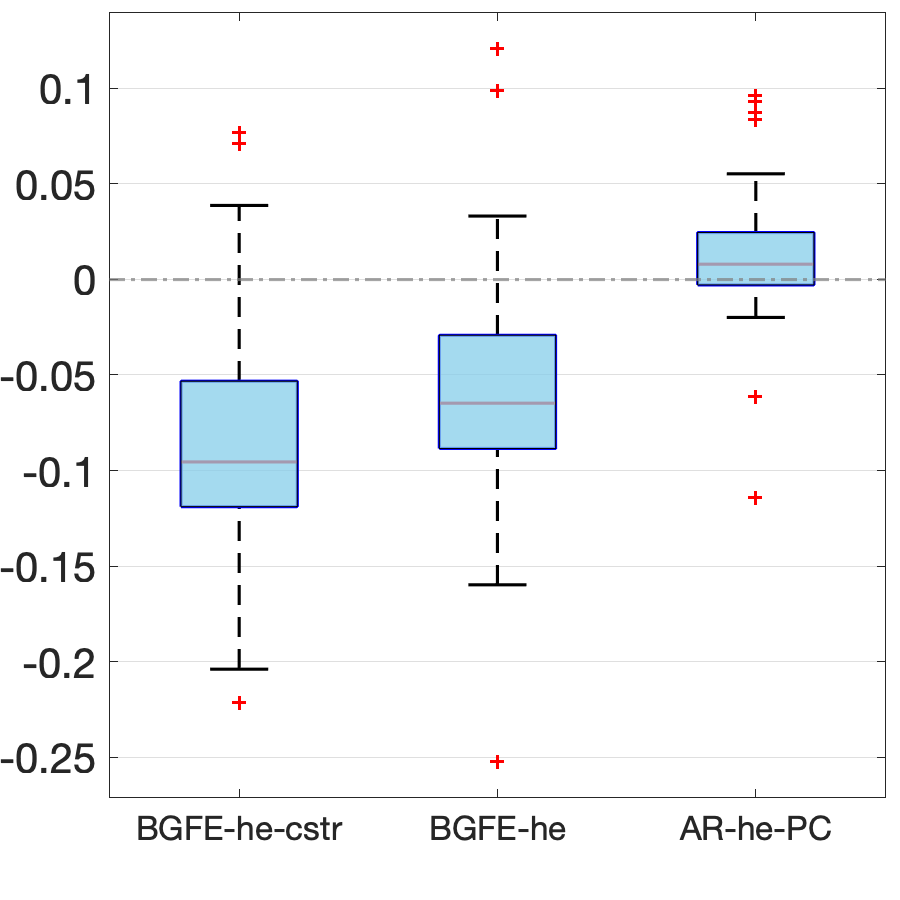
The revealing patterns of the density forecast are significantly distinct from those of the point forecast. Figure 7 depicts the log predictive score (LPS) for density forecast. The most notable pattern from the panel (a) is that the BGFE-he-cstr estimator, which incorporates prior knowledge, is dominating and outperforms the rest in over 80% of the samples. It emerges as the apparent winner in this case. Furthermore, when generating density forecast, the BGFE-ho and pooled OLS are not as accurate as they are in point forecast: they never have the lowest LPS across samples. This also confirms that the heteroscedasticity151515We provide more results in Section G.1.2 to explore the importance of heteroskedasticity in density forecast for the inflation. is a well-known feature of the inflation time series (Clark and Ravazzolo, 2015). In the boxplot, we ignore BGFE-ho and pooled OLS and show the differences in LPS between the respective estimators and the AR-he estimator. As LPS differences represent percentage point differences, BGFE-he-cstr can provide density forecasts that are up to 22% more accurate compared to the benchmark model. Finally, despite the fact that the BGFE-he-cstr and BGFE-he estimators are mainly based on the same algorithm, the use of prior knowledge on group pattern further enhances the performance, resulting in the BGFE-he-cstr estimator having a lower LPS and scoring the best model with the highest frequency.
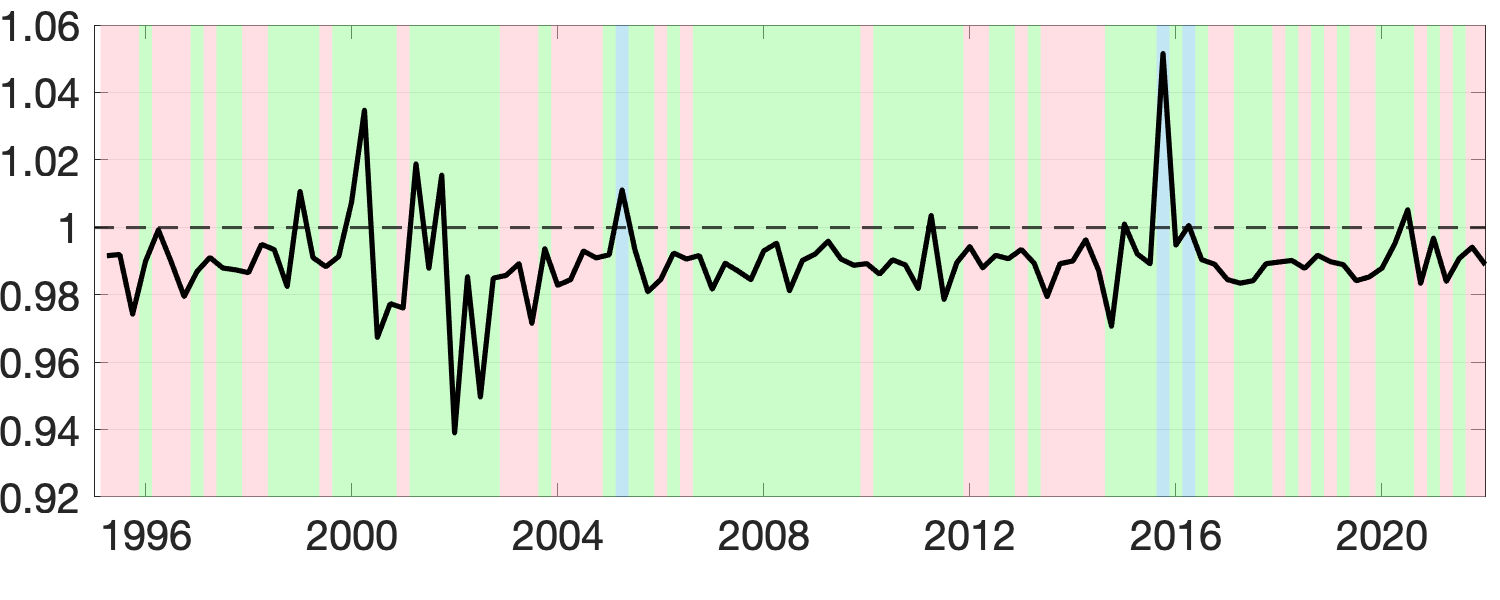
Next, we assess the value of adding prior information about groups by comparing the performance of the BGFE-he-cstr and BGFE-he estimators exclusively. The solid black line in Figure 8 represents the ratio of RMSE between BGFE-he-cstr and BGFE-he. The periods during which BGFE-he-cstr, BGFE-he, and all other estimators achieve the lowest RMSE are indicated by pink, blue, and green shaded areas, respectively. Though the BGFE-he-cstr estimator is not always the best across samples, the prior information improves the performance of the Bayesian grouped estimator. The BGFE-he-cstr estimator performs better than the BGFE-he estimator in most samples, with an average improvement of 2%.
Adding prior information on groups substantially improves the accuracy of density forecasts. Figure 9 shows the comparison between BGFE-he-cstr and BGFE-he in terms of the difference in LPS. We find the prior information valuable as BGFE-he-cstr outperforms BGFE-he in more than 98% of the samples. Clearly, the majority of the figure is covered by a pink background, showing that BGFE-he-cstr is typically the best choice. All of these facts demonstrate that adding prior informatio is favorable and essential, especially for density forecasting.
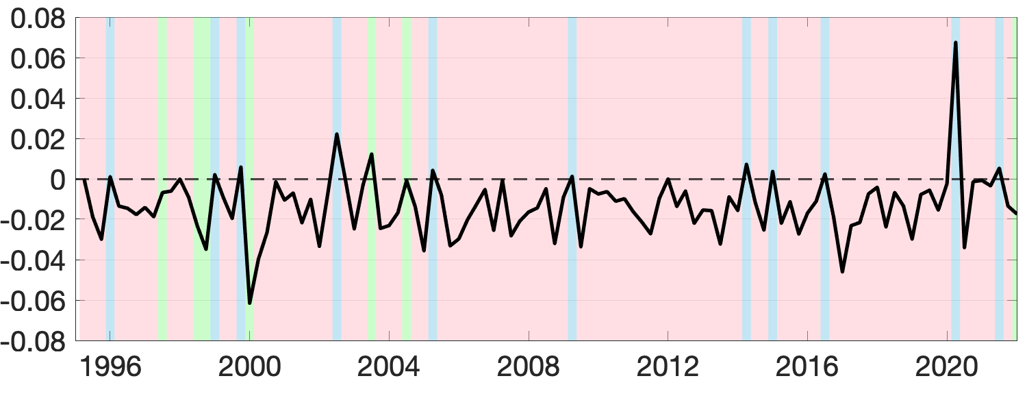
Having specified pairwise constraints across sub-indices, we provide a prior on that shrinks the group structure toward the eight expenditure categories with equal accuracy for all pairs inside each category. As Theorem 1 suggested, our prior specification essentially assumes that the prior probability of any two units that come from the same expenditure category being in the same group is equal, and the prior group pattern is actually the expenditure category. We now examine the posterior of group structure to demonstrate how the distribution of gets updated by data. In order to accomplish this, we construct a posterior similarity matrix (PSM), whose -element records the posterior probabilities of units and being in the same group. For illustrative purposes, we present the results for the last sample, in which we forecast CPI in August 2022. Figure 10 depicts the PSM generated by BGFE-he-crst for the series in the categories of Food and Beverages and Transportation. A darker block indicates a higher posterior probability of being in one group. A common pattern emerges: even though some sub-indices are joined together frequently, as shown in the dark diagonal blocks, it is extremely unlikely that all series within the same category belong to the same group. Some series have relatively low or zero probabilities of being grouped together, as suggested by the white and gray off-diagonal blocks. This indicates that the group structure based on official expenditure categories is not optimal, which may result in inaccurate forecasting. Instead, our suggested framework uses information from both prior beliefs and data to reinvent the group pattern, leading to improved forecasting performance.
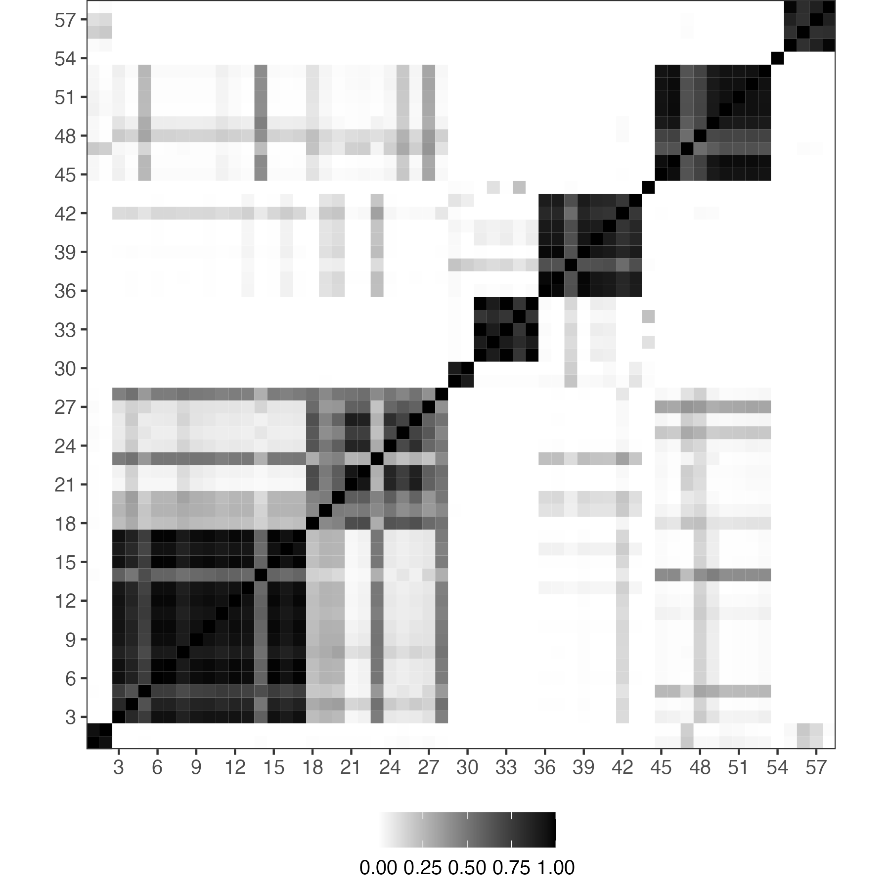
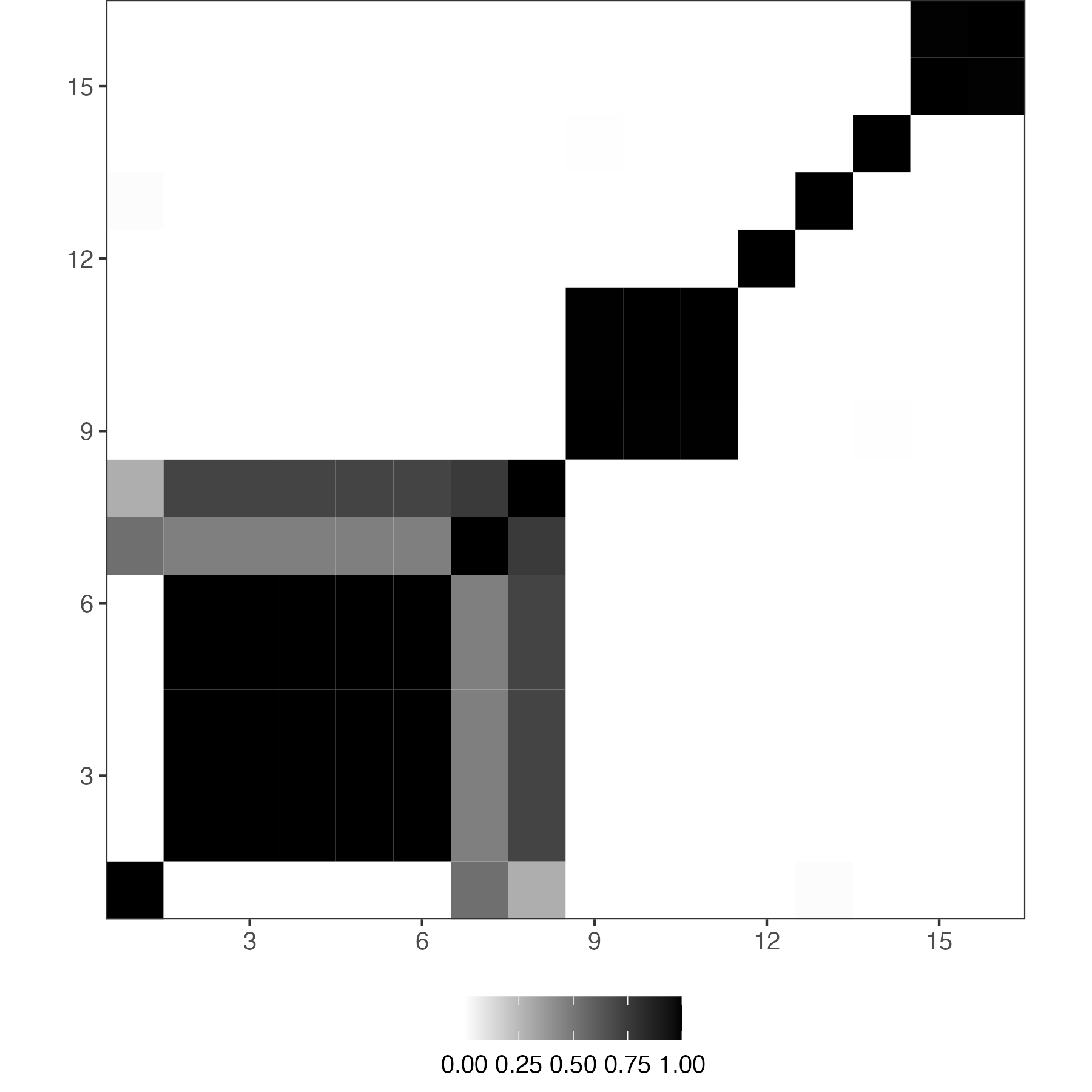
Notes: This is not the direct output of the algorithm, the ordering of series is changed so that cluster are lying on the diagonals.
Finally, we restrict our analysis to the point estimate of group partition, i.e., the single grouping solution, rather than the posterior over the whole universe of partitions. Figure 11 depicts the posterior point estimate of for the last sample ended in August 2022, derived using the approach described in Section 3.2. Eight expenditure categories are divided into twelve groups of varied sizes. Two different forms of groups are generated based on the arrangement of their components. Groups 2, 3, 4, and 5 contain sub-indices from a variety of categories, with no clear dominance. In contrast, the majority of the series in groups 1 and 8, for example, belong to a certain category. Group 1 may refer to a Food group, whereas group 8 is a Transportation group. The detailed group 8 components are depicted in Figure 12. There are seven sub-indices from Transportation, including car and truck rentals, gasoline (regular, midgrade, and premium), other motor fuels, airline fares, and ship fares, and one series from Housing - fuel oil (for residential heating). Clearly, all sub-indices share a common trend and have a close relationship with energy and oil prices, which have increased since the Pandemic. This is an example demonstrating that our proposed algorithm exploits cross-sectional information, not limited to our prior knowledge, and forms meaningful groups for forecasting.
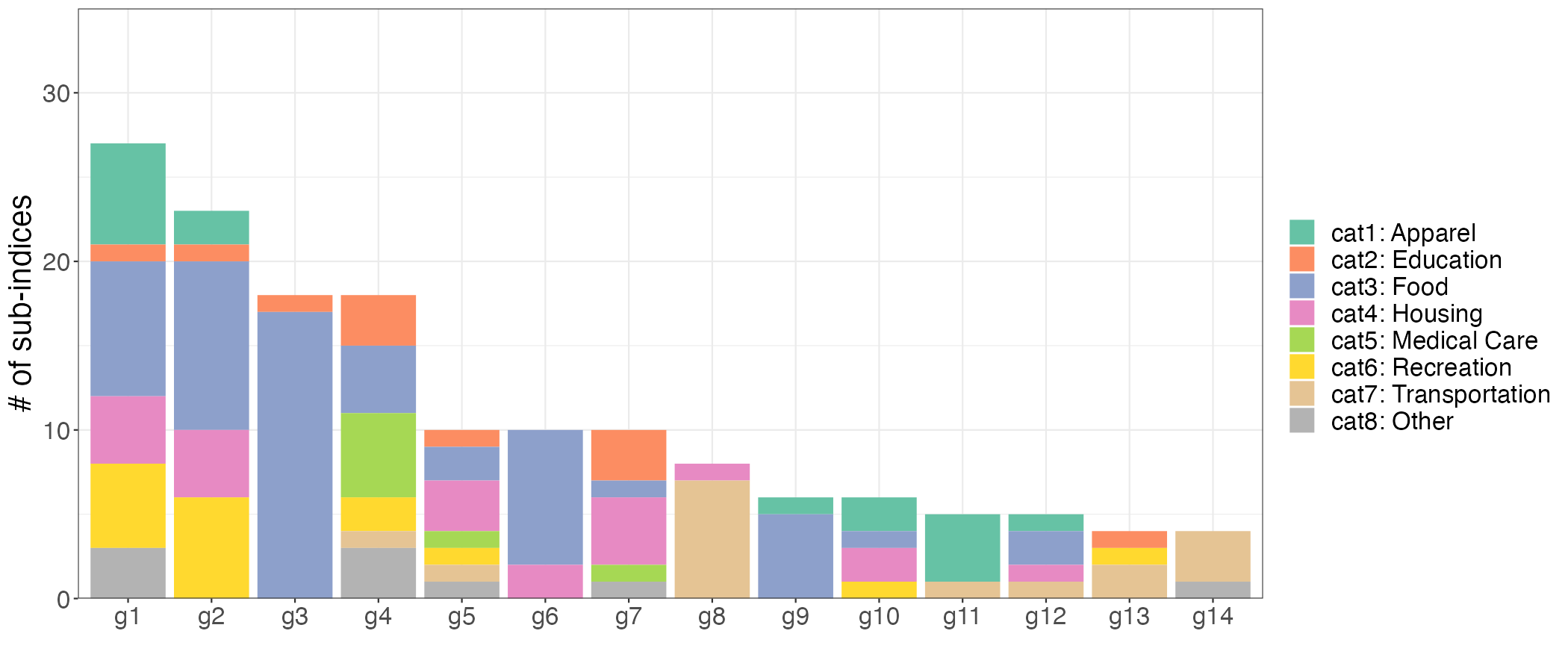
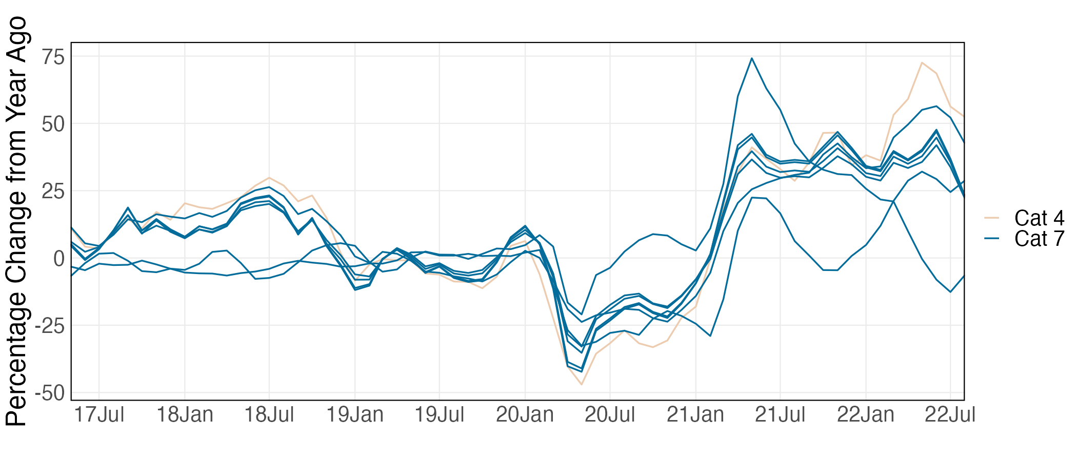
4.2.3 Impact of the Accuracy of Constraints
We examine how the accuracy of pairwise constraints influences the point estimate of group partitioning. For demonstration purposes, we restrict our analysis to PL constraints solely by setting and changing . We do not select the constant in the setup since it would balance the impact of the PL restrictions with a different level of accuracy. We set to 0.5. Again, PL constraints are derived from the official expenditure categories, with the assumption that all units within the same category are positive-linked with equal probability of being in the same group.
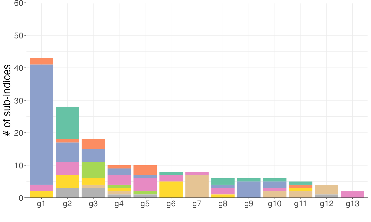
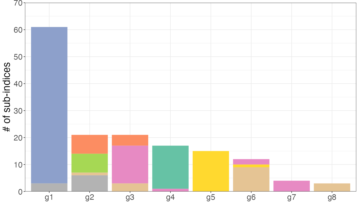
Figure 13 presents the point estimates of the group structure with two different levels of accuracy. The “weaker” PL constraints with , as shown in panel (a), demonstrate a limited influence of prior knowledge on the group structure. The eleven groups are composites of CPI sub-indices from the various categories, which is diverse from the official spending categories. Panel (b), on the other hand, illustrates the group structure with “stronger” PL constraints. By setting a high level of accuracy for PL constraints, such as , the prior knowledge dominates and pushes the group structure towards the official expenditure categories. As anticipated, panel (b) shows fewer groups, and the majority of CPI sub-indices within each group belong to the same category, bringing the group structure closer to that of the prior.
4.3 Income and Democracy
It is well-known in the literature that income per capita is strongly correlated with the level of democracy across countries. This strong empirical regularity is often known as ”modernization theory” or Lipset hypothesis (Lipset, 1959). The theory claims a causal relation: democratic regimes are created and consolidated in affluent societies (Lipset, 1959; Przeworski et al., 1995; Barro, 1999; Epstein et al., 2006).
In an influential paper, Acemoglu et al. (2008) challenge the casual effect of countries’ income on the level of democracy. They argue that it is essential to take into account other factors that affect both economic and political development simultaneously. Their analysis, based on panel data, indicates that the positive relationship between income and democracy disappears when fixed effects are included in the regression. They suggest that this finding is due to historical events, such as the end of feudalism, industrialization, or colonization, which have led countries to follow distinct paths of development. The fixed effects are meant to capture these persistent events. The finding is robust, as it holds for different measures of democracy, various econometric specifications, and additional covariates. Another study by Bonhomme and Manresa (2015) uses a different econometric model but arrives at the same conclusion. Their analysis highlights the presence of diverse group-specific paths of democratization in the data, consistent with the observation that regime types and transitions tend to cluster in time and space (Gleditsch and Ward, 2006; Ahlquist and Wibbels, 2012).
The seminal work of Acemoglu et al. (2008) has been subject to critical scrutiny by several recent works, including Moral-Benito and Bartolucci (2012), Benhabib et al. (2013), and Cervellati et al. (2014). Moral-Benito and Bartolucci (2012) contend that a nonlinear relationship between income and democracy exists, even after accounting for country-specific effects. They show that a positive income-democracy relationship holds only in countries with low levels of income. Benhabib et al. (2013) use panel estimation methods that adjust for the censoring of democracy measures at their upper and lower bounds and find that the positive relationship between income and democracy withstands the inclusion of country fixed effects. Cervellati et al. (2014) extend the linear estimation framework of Acemoglu et al. (2008) and unveil the presence of significant heterogeneity in the income effect on democracy across different subsamples. Specifically, they demonstrate that this effect exhibits an opposite sign for colonies and non-colonies, is substantially different from zero, and is of considerable magnitude. They also argue that the existence of a heterogeneous effect of income suggests that results from a linear framework, such as the finding of a zero effect, may lack robustness since they depend on the composition of the sample.
In this section, we contribute to the literature on the relationship between income and democracy by employing a novel grouped fixed-effects approach. Specifically, we expand on the econometric model proposed by Bonhomme and Manresa (2015) to incorporate group structure not only in time fixed-effects, but also in slope coefficients and the variance of errors. This more complex model allows for a more detailed analysis of the heterogeneous effects of income on democracy across different groups of countries. To identify these groups, we incorporate prior knowledge about the latent group structure by clustering countries based on either geographic location or initial levels of democracy score. By leveraging this information, we are able to identify a moderate number of groups, each of which exhibits a distinct path to democracy.
Our results indicate that the effect of income on democracy is highly varied across countries, a finding which is consistent with previous research by Cervellati et al. (2014). Furthermore, we find that the positive cumulative effect of income on democracy exists in groups of countries with a medium or relative low level of income, in line with the findings of Moral-Benito and Bartolucci (2012). However, the effect could be relatively small for some groups, suggesting that other factors beyond income may also play important roles in democratic development.
4.3.1 Model Specification and Data
Model: To accommodate richer assumptions on models for the real-world applications, we extend the baseline model in Chapter 1 either by adding common regressors and allowing for time-variation in the fixed-effects. Time-variation are essential to this analysis as they capture highly persistent historical shocks. Following Bonhomme and Manresa (2015), we introduce group-specific time patterns of heterogeneity and consider the following two specifications:
-
SP1:
Time-varying GFE + grouped slope coefficients
(4.14) -
SP2:
Time-varying GFE
(4.15)
where is the democracy score of country at time . The lagged value of democracy score is included to capture persistence in democracy and also potentially mean-reverting dynamics (i.e., the tendency of the democracy score to return to some equilibrium value for the country). The coefficient of main interest is and reflects the effect of the lagged value of income per capita on democracy. In addition, denote a set of group-specific time fixed-effects; is an error term with grouped variance , capturing additional transitory shocks to democracy and other omitted factors. We use the conjugate prior for all parameters, see details in Appendix B.
Specification 2 in (4.15) nests the linear dynamic panel data model in BM as a special case. If we assume homoskedasticity, it is the Equation (22) in BM. This specification enables us to reproduce BM’s results and provide fresh insight into their framework. Specification 1 in (4.14), on the other hand, generalizes specification 2 by introducing group-dependent slope coefficients. As we shall demonstrate in the following section, specification 1 yields a more refined group structure and provides a clearer view of the income effects.
Data: We use the Freedom House (FH) Political Rights Index as a benchmark for measuring democracy. To standardize the index, we normalize it between 0 and 1, with higher scores indicating higher levels of democracy. FH assesses a country’s political rights based on a checklist of questions, such as the presence of free and fair elections, the role of elected officials, the existence of competitive parties or other political groupings, the power of the opposition, and the extent of self-government or participation by minority groups. We measure countries’ income using the logarithm of GDP per capita, which is adjusted for purchasing power parity (PPP) in 1996 prices, using data from the Penn World Tables 6.1 (Heston et al., 2002). Details on the data can be found in Section 1 of Acemoglu et al. (2008), and all data in this section are from the replication files of Bonhomme and Manresa (2015).161616 https://www.dropbox.com/s/ssjabvc2hxa5791/Bonhomme_Manresa_codes.zip?dl=0 Our analysis is based on a five-year panel dataset that includes all independent countries since the postwar period, with observations taken every fifth year from 1970 to 2000. We chose this period for comparability with previous studies. The final dataset consists of a balanced panel of 89 countries.
Prior group structure: We propose two prior grouping strategies as specified below and assume all units within the same prior group are presumed to be positive-linked, while units from different prior groups are believed to be negative-linked.
-
(i)
Given the countries available in the dataset, we form six groups according to their geographic locations:171717The regions are assigned by the Economist Intelligence Unit, and may slightly differ from conventional classifications. (1) North America; (2) Europe; (3) Latin America and the Caribbean; (4) Asia and Australasia; (5) Sub-Saharan Africa; (6) Middle East and North Africa. We refer this prior to geo-prior.
-
(ii)
Alternately, countries could be categorized according to their initial level of democracy in year 1970. As the Freedom House Index has six possible values, we cluster countries into three primary groups with a reasonable number of countries in each: (1) low democracy, 0 or 0.166; (2) medium democracy, 0.333, 0.5, or 0.667; (3) high democracy, 0.833 or 1. We refer this prior to dem-prior.
Figure 14 presents the world maps with countries colored differently according to their respective groups. The panel on the left illustrates the geographic groups, while the panel on the right depicts the democratic groups. All gray nations/regions are excluded from the dataset. We concentrate primarily on the first pre-grouping strategy, as it needs no country-specific knowledge beyond geographic information. We then compare the results using different pre-grouping strategies in Section 4.3.3.
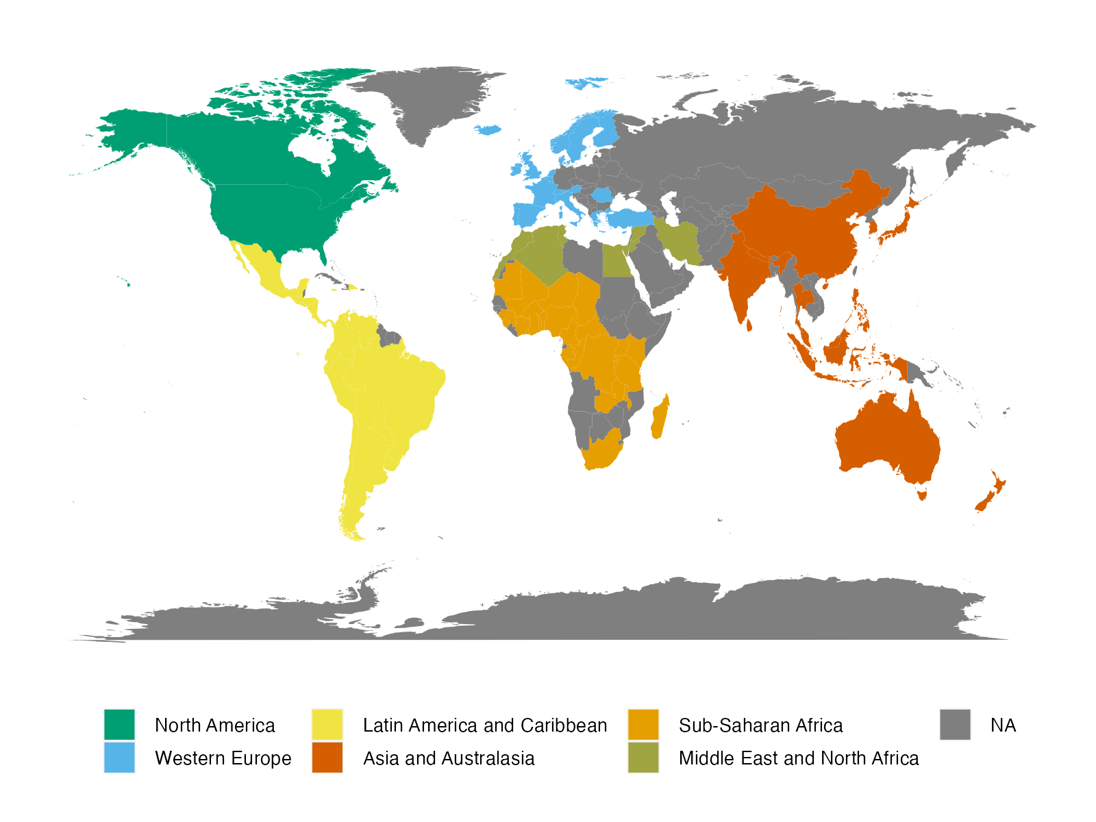
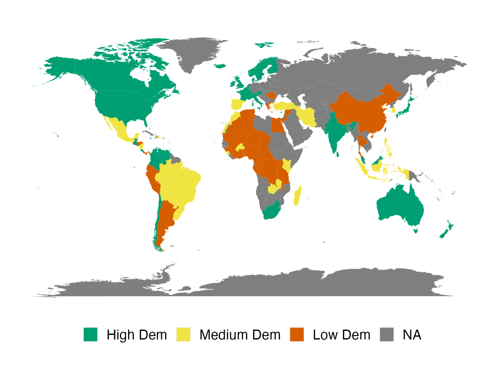
4.3.2 Results
Specification 1: We begin with specification 1 where group-specific slope coefficients are allowed and new findings emerge. Table 1 presents the posterior probability of the number of groups utilizing various estimators. BGFE-ho creates more than 5 groups in all posterior draws. Intriguingly, accounting for heteroskedasticity drastically reduces the number of groups, with BGFE-he identifying four groups. Adding pairwise constraints based on geographic information increases the number of groups to five, whereas six groups are expected in the prior.
| BGFE-he-cstr | BGFE-he | |
| 0.000 | 0.000 | |
| 0.000 | 1.000 | |
| 1.000 | 0.000 | |
| 0.000 | 0.000 |
The marginal data density (MDD) of each estimator in Table 2 provides some insight on different models. Among all the estimators, the BGFE-ho estimator has the lowest MDD; it is even lower than that of specification 1. BGFE-he-cstr and BGFE-he, on the other hand, benefit from the introduction of group-specific slope coefficients, since both achieve substantially greater MDD than in specification 1. BGFE-he-cstr has the highest MDD since the pairwise constraints give direction on grouping and identify the ideal group structure, which BGFE-he cannot uncover without our prior knowledge.
| BGFE-he-cstr | BGFE-he | BGFE-ho | |
| SP1 | 544.324 | 501.904 | 327.077 |
| SP2 | 413.476 | 381.218 | 368.918 |
We concentrate on the BGFE-he-cstr estimator and use the approach outlined in Section 3.2 to identify the unique group partitioning . The left panel of Figure 15 presents the world map colored by , while the right panel present the group-specific averages of democracy index over time. The estimated group structure features five distinct groups which we refer to as the “high-democracy”, “low-democracy”, “flawed-democracy”, “late-transition” and “progressive-transition” group, respectively. With the exception of the “flawed-democracy” and “progressive-transition” group, the group-specific averages of the democracy index are comparable to those in BM for all other groups. BGFE-he-cstr does not identify the ”early transition” group in comparison to BM but instead produces two new groups. Group 3 (”flawed-democracy”) comprises primarily of relatively democratic but not the most democratic nations, including India, Sri Lanka, and Venezuela, among others. Group 5 (”progressive transition”) contains 30 countries that have had a steady expansion of democracy, including Argentina, Greece, and Panama. Consequently, by incorporating group-specific slope coefficients, we recover a more refined group structure than that of BM.

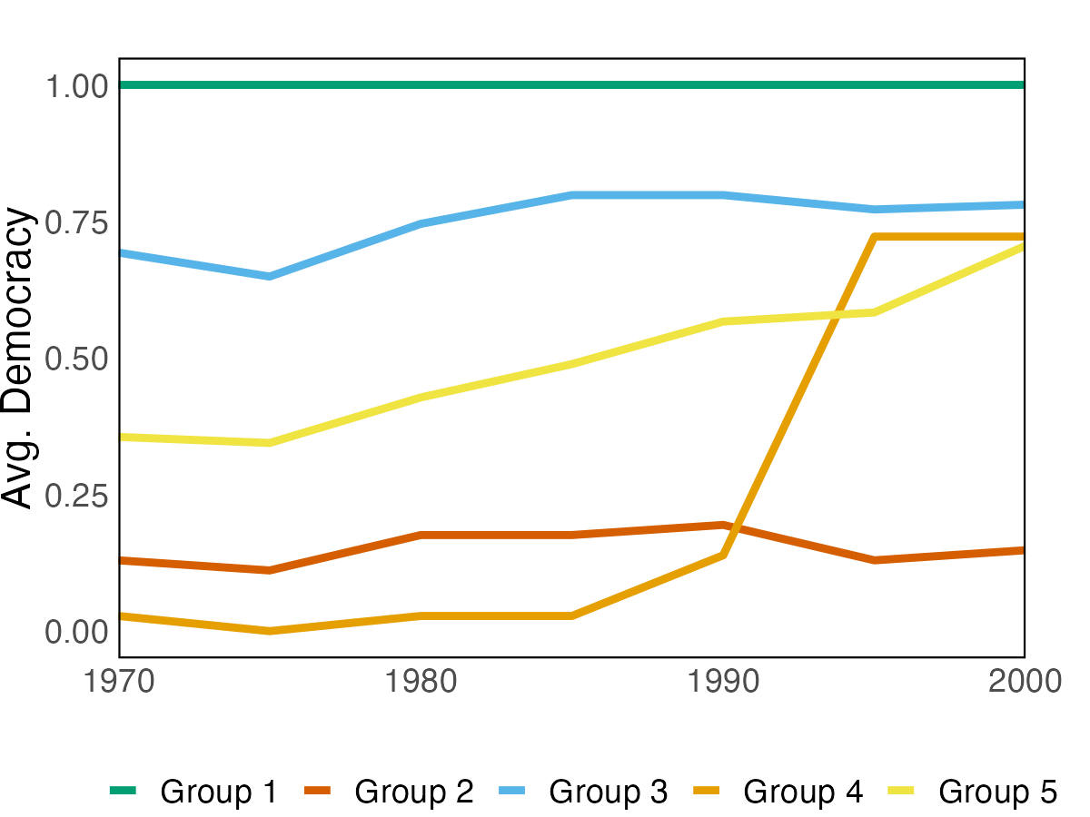
Table 3 presents the posterior mean and 90% credible set for each coefficient across all groups, with fixed at the point estimate . The key feature of using the specification 1 is that we are able to see distinct (cumulative) income effects across groups as group-specific coefficients are allowed.
The effect of income on democracy is negligible for group 1 (”full-democracy”) and group 4 (”late-transition”) as the posterior means of are close to 0 and the associated credible intervals for contain 0. Group 1, which we refer to as the ”full-democracy” group, mostly contains high-income, high-democracy countries. It includes the United States, Canada, UK, most of European countries, Australia, and New Zealand, but also Costa Rica and Uruguay. These country kept their democracy index at the highest level throughout the sample, demonstrating that income has no effect on democracy. Group 4 is referred to as the ”late-transition” group, which consists of Benin, Central African Republic, Mali, Malawi, Niger, and Romania. The transition to democracy for countries in group 4 was primarily driven by historical events in the 90s: Romania began a transition towards democracy after the 1989 Revolution; all other countries involved in the third wave of democratization in sub-Saharan Africa beginning in 1989. The impact of historical events is primarily captured by time fixed-effects, as the credible intervals for and well cover zero.
Group 2 (”low-democracy”) and group 3 (”flawed-democracy”) are two groups that have stable Freedom House scores. Lagged democracy is highly significant and indicates that there is a considerable degree of persistence in democracy. Log income per capita is also significant and illustrates the well-documented positive relationship between income and democracy. Though statistically significant, the effect of income is quantitatively small. For example, the coefficient of 0.055 for the group 3 implies that a 10 percent increase in GDP per capita is associated with an increase in the Freedom House score of 0.0055, which is very small. Group 2 includes low-democratic countries, China, Singapore, Iran, and a fraction of African countries, whose Freedom House scores remain relatively low throughout the sample. Countries in group 3, however, have Freedom House score stay in the relatively high level. The group covers countries with almost democratic but minor flaws in certain aspects, including India, Japan, South Korea, Finland, Sweden, and Portugal, among others. The cumulative income effects for these two groups are, however, different - it is negligible for group 2 (0.079) and modest for group 3 (0.244). Group 5 (”progressive-transition”), on the other hand, experiences a continuous increase in Freedom House score from a 0.35 in 1970 to 0.7 in 2020. It has the largest positive income coefficient, although the cumulative income effect is modest (0.156).
| Lagged democracy () | Lagged Income () | Income Effect () | Error variance () | |||||
| Coef. | Cred. Set | Coef. | Cred. Set | Coef. | Cred. Set | Coef. | Cred. Set | |
| Group 1 (16) | 0.058 | [-0.263, 0.360] | 0.000 | [-0.012, 0.012] | 0.000 | [-0.013, 0.013] | 0.001 | [0.001, 0.001] |
| Group 2 (18) | 0.484 | [ 0.354, 0.606] | 0.041 | [ 0.019, 0.062] | 0.079 | [ 0.044, 0.117] | 0.010 | [0.008, 0.011] |
| Group 3 (19) | 0.775 | [ 0.703, 0.850] | 0.055 | [ 0.031, 0.078] | 0.249 | [ 0.143, 0.352] | 0.013 | [0.011, 0.016] |
| Group 4 (6) | -0.178 | [-0.468, 0.115] | -0.025 | [-0.066, 0.017] | -0.020 | [-0.054, 0.015] | 0.008 | [0.005, 0.011] |
| Group 5 (30) | 0.206 | [ 0.091, 0.310] | 0.125 | [ 0.090, 0.163] | 0.157 | [ 0.118, 0.199] | 0.057 | [0.048, 0.066] |
| Pooled OLS | 0.667 | [ 0.614, 0.717] | 0.081 | [ 0.064, 0.099] | 0.244 | [ 0.207, 0.281] | 0.039 | [0.035, 0.043] |
Figure 16 depicts the historical average log income for each group of countries between 1970 and 2000. Except for the high income group (group 1) and low income group (group 4), all other three groups with medium or relatively low levels of income reveal positive cumulative income effect, as indicated in Table 3. This finding is generally in line with the results of Moral-Benito and Bartolucci (2012), who observe a positive effect in low-income nations. Notice that, their definition of low-income country is quite board, encompassing countries with a GDP per capita below the 80th percentile of the empirical cross-sectional density.. As a result, beside six counties in the group 4 that had the lowest income on average, other countries fit within this definition and confirm that the positive income effect is not prevalent in high-income countries.
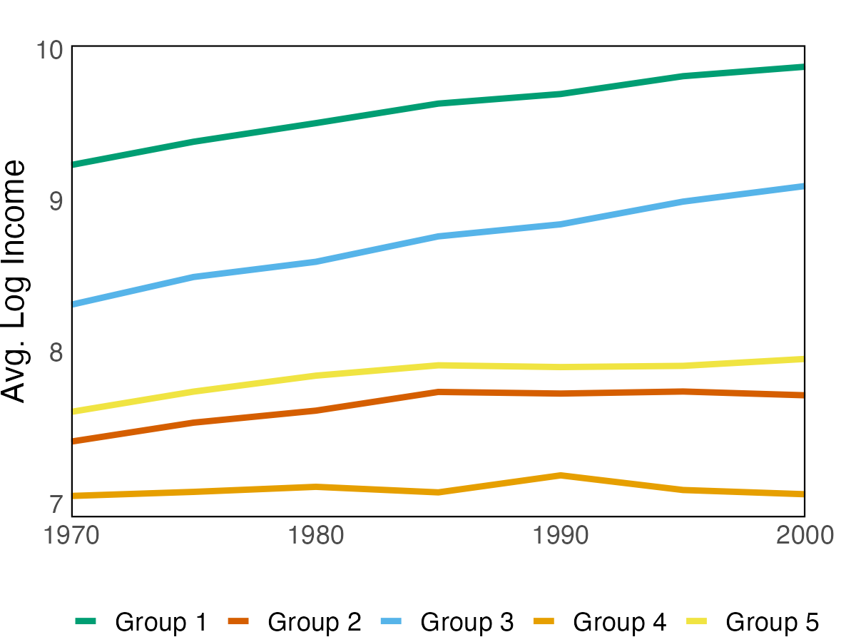
Specification 2: The results for specification 2 are reported in Appendix G.2. In short, the results are comparable to the key findings in BM. BGFE-ho in specification 1 is identical to the main model in BM; it produces eight groups, which is consistent with the upper bound on the number of groups in BM based on BIC. BGFE-he-cstr, on the other hand, is more preferable and has the highest marginal data density as shown in Table 2. The point estimate of group partitioning based on BGFE-he-cstr consists of four groups that all have the similar pattern as BM’s group structure. This justifies BM’s subjective choice of four groups. Regarding the estimated coefficients, there is moderate persistence and a positive effect of income on democracy, but the cumulative effect of income is quantitatively small: .
4.3.3 Impacts of Different Pre-Grouping Strategies
All results presented thus far are based on pairwise constraints derived from spatial information. We now implement the alternative pre-grouping strategy based on the initial level of democracy. We stick with the BGFE-he-cstr estimator under specification 1.
Different pre-grouping strategies yields different estimates of group patterns. We consider the BGFE-he estimator with three prior group structures: geo-prior, dem-prior, and no prior knowledge, with point estimates of the group partition presented in panel (17(a)), (17(b)), and (17(c)) of Figure 17, respectively. Geo-prior and dem-prior produce comparable group structures, however certain nations are assigned to distinct groups.. They are encircled in the black dashed rectangle, including Portugal, Spain, Romania, Mali, Niger, Central African Republic, Benin, Malawi, and Jordan. Another country is South Korea. As depicted in panel (17(c)), without any prior knowledge of groups, the group pattern is quite different, particularly for countries in Asia, Africa, and Latin America.
The difference in group patterns result in discrepancies in MDD, which are listed in Table 4. The BGFE-he estimator with geo-prior has the highest MDD in both specifications, whereas the dem-prior is only informative in specification 1 in comparison to the BGFE-he estimator without prior knowledge.
| geo-prior | dem-prior | no prior | |
| SP1 | 544.324 | 527.517 | 501.904 |
| SP2 | 413.476 | 309.369 | 381.218 |
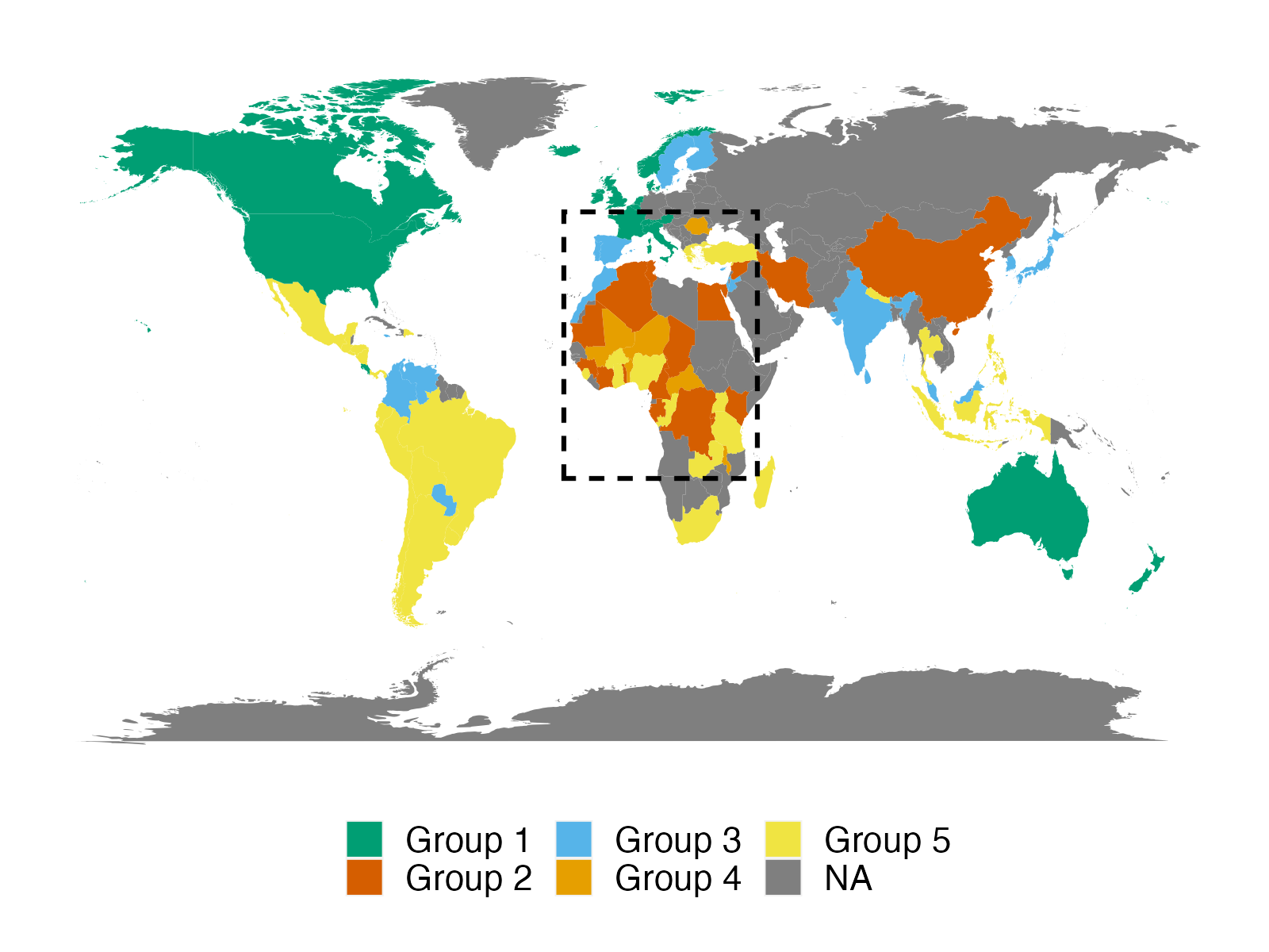
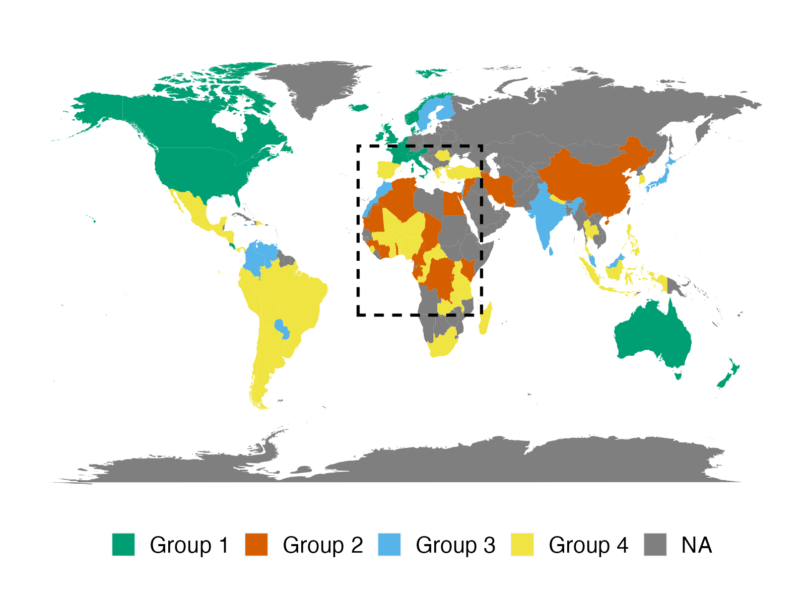
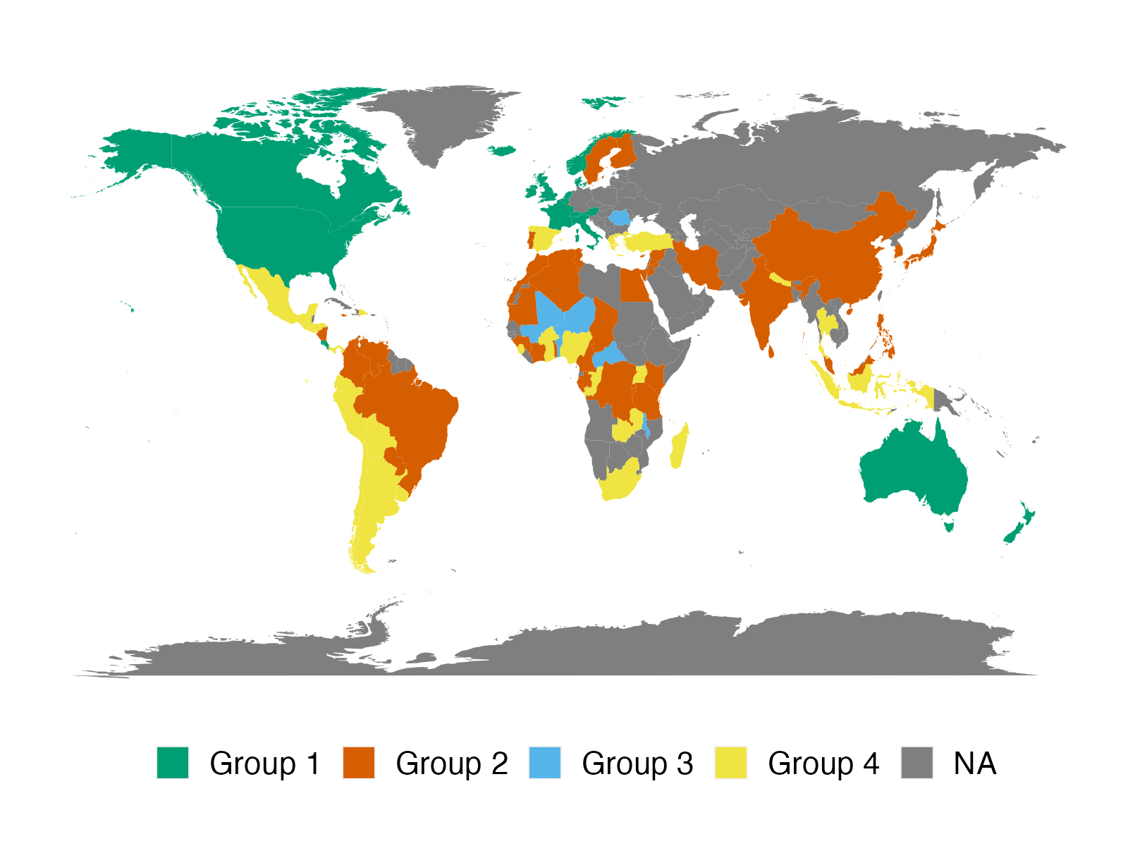
Using the initial level of democracy as prior knowledge results in four groups, as indicated in the panel (17(b)). The dem-prior has two major impacts on the group structure comparing with the geo-prior. It combines the “late-transition” group (group 4 in geo-prior) with the “progressive-transition” group (group 5 in geo-prior) to form a bigger and boarder “progressive-transition” group. Additionally, Portugal and Spain are no longer categorized as “flawed-democracy” countries, but rather as “progressive-transition” group in a boarder sense. In terms of the posterior estimates, as shown in Table 5, we observe similar value for the first three groups because they are merely subject to minor changes in the group structure. However, as “late-transition” and “progressive-transition” groups are agglomerated together under the dem-prior, the income effects of countries in the new group becomes larger, forcing some countries to exhibit strong and positive effects even though they are not under the geo-prior.
| Lagged democracy () | Lagged Income () | Income Effect () | Error variance () | |||||
| Coef. | Cred. Set | Coef. | Cred. Set | Coef. | Cred. Set | Coef. | Cred. Set | |
| Group 1 (16) | 0.062 | [-0.262, 0.369] | 0.000 | [-0.012, 0.012] | 0.000 | [-0.014, 0.013] | 0.001 | [0.001, 0.001] |
| Group 2 (19) | 0.513 | [ 0.395, 0.640] | 0.043 | [ 0.022, 0.064] | 0.087 | [ 0.047, 0.126] | 0.010 | [0.008, 0.012] |
| Group 3 (15) | 0.802 | [ 0.704, 0.904] | 0.040 | [ 0.016, 0.064] | 0.223 | [ 0.079, 0.337] | 0.012 | [0.009, 0.015] |
| Group 4 (39) | 0.302 | [ 0.205, 0.388] | 0.120 | [ 0.092, 0.151] | 0.172 | [ 0.136, 0.210] | 0.054 | [0.047, 0.062] |
| Pooled OLS | 0.667 | [ 0.614, 0.717] | 0.081 | [ 0.064, 0.099] | 0.244 | [ 0.207, 0.281] | 0.039 | [0.035, 0.043] |
5 Extensions
Within the domain of panel data models, the proposed constrained-based BGFE framework can be extended in multiple directions to allow for more subtle group structures or more covariates. In addition, the DP prior with soft pairwise constraints also applies to other related topics and models, such as clustering problems, heterogeneous treatment effects, and panel VARs.
5.1 Subtle Group Structure
Through the Dirichlet process defines a prior that possesses the clustering property and is flexible enough to incorporate pairwise constraints, the group structure itself is elementary. Aside from our prior belief on the group, the group structure, which is introduced in all and , is entirely governed by the stick-breaking process defined in Equation (2.13). The stick length , on which we have a prior, is independent of any regressors or time. Consequently, each unit is associated with a single group, and the membership remains constant across time.
To create an even more flexible and richer group structure, we provide insight into three possible extensions, each of which requires a set of more distinctive nonparametric priors. (1) overlapping group and (2) time-varying group and (3) dependent group.
Overlapping group structures allow for multi-dimensional grouping. This is a natural extension without having to greatly modify the proposed DP prior. Following Cheng et al. (2019), each of ’s and may have its own group structure and a separate Dirichlet process is specified to each of them. As a result, units simultaneously belong to multiple groups based on the heterogeneous effects among regressors or cross-sectional heteroskedasticity.
Time-varying group structures allow the membership of the group to change over time. We could replace the DP by variants of the hierarchical Dirichlet process (Teh et al., 2006) to achieve this feature. In short, the hierarchical Dirichlet process (HDP), a nonparametric Bayesian approach to clustering grouped data, is now the foundation of the prior. The time dimension naturally divides the panel data into groups, and a Dirichlet process is assumed for each group, with all Dirichlet processes having the same base distribution, which is distributed according to a global base distribution. The HDP allows each group to have its own cluster, but most importantly, these clusters are shared across groups. This lays the groundwork for time-varying group structures, as it assumes that the number of clusters remains constant over time, while cluster memberships are subject to change. Variants of the HPD are then proposed to capture the time-persistence in group structures, including dynamic HDP (Ren et al., 2008) and sticky HDP (Fox et al., 2008, 2011). A closely related area in the frequentists’ methods is to identify structure breaks in parameters with grouped patterns, see Okui and Wang (2021); Lumsdaine et al. (2022).
Dependent group structures allow the prior group probability to rely directly on a collection of characteristics. The dependence is introduced through a modification of the stick-breaking representation for DPs, where the group probabilities vary with the characteristics. Rodriguez and Dunson (2011) introduced the probit-stick breaking (PSB) process where the Beta random variables are replaced by normally distributed random variables transformed using the standard normal CDF. The PSB is defined by,
| (5.1) |
where stochastic function is drawn from Gaussian process for and is the set of characteristics that are informative to the latent group. Other forms of dependence are also available, see Quintana et al. (2022) for a comprehensive review. A caveat of this approach is that analysis of group structure is confined to observed by the researcher. The approach requires researchers to know possible key characteristics, be able to observe them and ensure they are informative. In many cases, however, these characteristics might be hard to justify by researchers.
5.2 Beyond Panel Data Models
Although we concentrate on panel data model, our framework of the DP prior with soft pairwise constraints applies to other models where the group structure are crucial.
Gaussian Mixture Model
If we ignore covariates and focus exclusively on group membership, we essentially face a classical clustering problem with an infinite-dimensional mixture model. A typical probabilistic model is the infinite Gaussian mixture model (Rasmussen, 1999), where the data itself is assumed to be drawn from a mixture of Gaussian components
| (5.2) |
where are the mixture weights. With soft pairwise constraints, observations are clustered in accordance with prior belief.
Heterogeneous Treatment Effects
Following the potential outcomes framework of Rubin (1974), we posit the existence of potential outcomes and corresponding respectively to the response the th subject would have experienced with and without the treatment, and define the treatment effect at as
| (5.3) |
Previous works on Bayesian analysis for the treatment effects include Chib and Hamilton (2000, 2002); Chib and Jacobi (2007); Chib (2007); Heckman et al. (2014), etc. Another strand of literature propose to estimate (5.3) by using several machine learning algorithms (Hill, 2011; Athey and Imbens, 2016; Wager and Athey, 2018). These methods are built on the idea that researchers find the subsamples across which the effect of a treatment differs out of all possible subsamples on the basis of the values of . Instead of trying to discover valid subsets of the data, Shiraito (2016) directly models the outcome as a function of the treatment and pre-treatment covariates and estimate of the distribution of conditional average treatment effects (CATE) across units by employing the Dirichlet process.
| (5.4) |
where is the binary treatment variable. Our approaches fit in this methods by adding side information on the treatment groups into the prior.
Panel VARs
Panel VARs (Holtz-Eakin et al., 1988; Canova and Ciccarelli, 2013, and references therein.) has been widely used in macroeconomic analysis and policy evaluations to capture the interdependency across sectors, markets, and countries. Nevertheless, the large dimension of panel VARs typically makes the curse of dimensionality a severe problem. Billio et al. (2019) propose nonparametric Bayesian priors that cluster the VAR coefficients and induce group-level shrinkage. Our paradigm with the DP prior with soft pairwise constraints is applicable to their method and injects prior information on groups into the underlying Granger causal networks.
Panel VARs have the same structure as VAR models, in the sense that all variables are assumed to be endogenous and interdependent, but a cross-sectional dimension is added to the representation. Thus, let be the stacked version of , the vector of variables for each unit , i.e., . Then a panel VAR is
| (5.5) |
where is a vector of idiosyncratic errors and and are matrices of coefficients.
The main feature of Billio et al. (2019) is to specify a prior that blends the DP prior with Lasso prior for each of and , such that the VAR coefficients are either shrunk toward 0 or clustered at multiple non-zero locations. Our proposed DP prior with soft pairwise constraints, in the meantime, fit into their framework by replacing the original DP prior and permitting richer structure within each coefficient matrix. As the nonzero coefficients form Granger causal networks, equipping with soft pairwise constraints may result in a more plausible network by taking researchers’ expertise into account.
6 Concluding Remarks
This paper proposes a Bayesian framework for estimating and forecasting in panel data models when prior group knowledge is available and informative for the group pattern. We include prior knowledge in the form of soft pairwise constraints into the Dirichlet process prior. Then, an intuitive and coherent prior is presented. The constrained grouped estimator proposed examines both heteroskedasticity and heterogeneous slope coefficients to endogenously reveal group structure. Our framework immediately estimates the number of groups as opposed to relying on ex-post model selection, and the structure of pairwise restrictions circumvents the computational difficulties and limitations that afflict conventional approaches. In addition, when utilizing small-variance asymptotics, the suggested Gibbs sampler with pairwise constraint contains a clustering procedure comparable to that of the constrained KMeans algorithm. In Monte Carlo simulations, we demonstrate that constrained Bayesian grouped estimators outperform conventional estimators even in the presence of incorrect prior knowledge. Our empirical application to forecasting sub-indices of CPI inflation rates demonstrates that incorporating prior knowledge on the latent group structure yields more accurate density predictions. The better forecasting performance is mostly attributable to the key characteristics: nonparametric Bayesian prior and grouped cross-sectional variance. The method proposed in this paper is applicable beyond forecasting. In a second application, we revisit the relationship between a country’s income and its democratic transition, where estimation of heterogeneous parameters is the object of interest. We recover a reasonable cluster pattern with a moderate number of groups and identify heterogeneous income effects on democracy.
The current work raises exciting questions for future research. It is desirable to investigate overlapping group structures, in which a unit might belong to many groups. This would allow us to increase the flexibility of a panel data model, potentially enhancing its predictive performance. Second, the assumption that an individual cannot change its group identity for the entire sample time can be amended, resulting in a specification that is even more flexible. Thirdly, our method is applicable to other econometric models, such as panel VARs with latent group structures in macro series.
References
- Acemoglu et al. (2008) Acemoglu, D., S. Johnson, J. A. Robinson, and P. Yared (2008): “Income and Democracy,” American Economic Review, 98, 808–42.
- Aguilar and Boot (2022) Aguilar, J. and T. Boot (2022): “Grouped Heterogeneity in Linear Panel Data Models with Heterogeneous Error Variances,” Available at SSRN 4031841.
- Ahlquist and Wibbels (2012) Ahlquist, J. S. and E. Wibbels (2012): “Riding the Wave: World Trade and Factor-Based Models of Democratization,” American Journal of Political Science, 56, 447–464.
- Aldous (1985) Aldous, D. J. (1985): “Exchangeability and Related Topics,” in École d’Été de Probabilités de Saint-Flour XIII—1983, Springer, 1–198.
- Anderson and Hsiao (1982) Anderson, T. W. and C. Hsiao (1982): “Formulation and Estimation of Dynamic Models using Panel Data,” Journal of Econometrics, 18, 47–82.
- Ando and Bai (2016) Ando, T. and J. Bai (2016): “Panel Data Models with Grouped Factor Structure under Unknown Group Membership,” Journal of Applied Econometrics, 31, 163–191.
- Antoniak (1974) Antoniak, C. E. (1974): “Mixtures of Dirichlet Processes with Applications to Bayesian Nonparametric Problems,” The Annals of Statistics, 2, 1152–1174.
- Ascolani et al. (2022) Ascolani, F., A. Lijoi, G. Rebaudo, and G. Zanella (2022): “Clustering Consistency with Dirichlet Process Mixtures,” arXiv preprint arXiv:2205.12924.
- Athey and Imbens (2016) Athey, S. and G. Imbens (2016): “Recursive Partitioning for Heterogeneous Causal Effects,” Proceedings of the National Academy of Sciences, 113, 7353–7360.
- Atkeson et al. (2001) Atkeson, A., L. E. Ohanian, et al. (2001): “Are Phillips Curves Useful for Forecasting Inflation?” Federal Reserve Bank of Minneapolis Quarterly Review, 25, 2–11.
- Barro (1999) Barro, R. J. (1999): “Determinants of Democracy,” Journal of Political economy, 107, S158–S183.
- Basu et al. (2002) Basu, S., A. Banerjee, and R. Mooney (2002): “Semi-Supervised Clustering by Seeding,” in Proceedings of 19th International Conference on Machine Learning, Citeseer.
- Basu et al. (2004a) Basu, S., A. Banerjee, and R. J. Mooney (2004a): “Active Semi-Supervision for Pairwise Constrained Clustering,” in Proceedings of the 2004 SIAM international conference on data mining, SIAM, 333–344.
- Basu et al. (2004b) Basu, S., M. Bilenko, and R. J. Mooney (2004b): “A Probabilistic Framework for Semi-Supervised Clustering,” in Proceedings of the Tenth ACM SIGKDD International Conference on Knowledge Discovery and Data Mining, 59–68.
- Benhabib et al. (2013) Benhabib, J., A. Corvalan, and M. M. Spiegel (2013): “Income and Democracy: Evidence from Nonlinear Estimations,” Economics Letters, 118, 489–492.
- Bernanke (2007) Bernanke, B. S. (2007): “Inflation Expectations and Inflation Forecasting,” in Speech at the Monetary Economics Workshop of the National Bureau of Economic Research Summer Institute, Cambridge, Massachusetts, vol. 10.
- Bilenko et al. (2004) Bilenko, M., S. Basu, and R. J. Mooney (2004): “Integrating Constraints and Metric Learning in Semi-Supervised Clustering,” in Proceedings of the 21st International Conference on Machine Learning, 81–88.
- Billio et al. (2019) Billio, M., R. Casarin, and L. Rossini (2019): “Bayesian Nonparametric Sparse VAR Models,” Journal of Econometrics, 212, 97–115.
- Blackwell and MacQueen (1973) Blackwell, D. and J. B. MacQueen (1973): “Ferguson Distributions via Pólya Urn Schemes,” The Annals of Statistics, 1, 353–355.
- Bonhomme et al. (2022) Bonhomme, S., T. Lamadon, and E. Manresa (2022): “Discretizing Unobserved Heterogeneity,” Econometrica, 90, 625–643.
- Bonhomme and Manresa (2015) Bonhomme, S. and E. Manresa (2015): “Grouped Patterns of Heterogeneity in Panel Data,” Econometrica, 83, 1147–1184.
- Buchinsky et al. (2005) Buchinsky, M., J. Hahn, and V. Hotz (2005): “Cluster Analysis: A Tool for Preliminary Structural Analysis,” Unpublished manuscript.
- Canova and Ciccarelli (2013) Canova, F. and M. Ciccarelli (2013): “Panel Vector Autoregressive Models: A Survey,” in VAR Models in Macroeconomics–New Developments and Applications: Essays in Honor of Christopher A. Sims, Emerald Group Publishing Limited.
- Cervellati et al. (2014) Cervellati, M., F. Jung, U. Sunde, and T. Vischer (2014): “Income and Democracy: Comment,” American Economic Review, 104, 707–719.
- Chamberlain (1980) Chamberlain, G. (1980): “Analysis of Covariance with Qualitative Data,” The Review of Economic Studies, 47, 225–238.
- Cheng et al. (2019) Cheng, X., F. Schorfheide, and P. Shao (2019): “Clustering for Multi-Dimensional Heterogeneity,” Manuscript.
- Chetty et al. (2014) Chetty, R., J. N. Friedman, and J. E. Rockoff (2014): “Measuring the Impacts of Teachers I: Evaluating Bias in Teacher Value-Added Estimates,” American Economic Review, 104, 2593–2632.
- Chib (2007) Chib, S. (2007): “Analysis of Treatment Response Data without the Joint Distribution of Potential Outcomes,” Journal of Econometrics, 140, 401–412.
- Chib and Hamilton (2000) Chib, S. and B. H. Hamilton (2000): “Bayesian Analysis of Cross-Section and Clustered Data Treatment Models,” journal of Econometrics, 97, 25–50.
- Chib and Hamilton (2002) ——— (2002): “Semiparametric Bayes Analysis of Longitudinal Data Treatment Models,” Journal of Econometrics, 110, 67–89.
- Chib and Jacobi (2007) Chib, S. and L. Jacobi (2007): “Modeling and Calculating the Effect of Treatment at Baseline from Panel Outcomes,” Journal of Econometrics, 140, 781–801.
- Clark and Ravazzolo (2015) Clark, T. E. and F. Ravazzolo (2015): “Macroeconomic Forecasting Performance under Alternative Specifications of Time-Varying Volatility,” Journal of Applied Econometrics, 30, 551–575.
- Cytrynbaum (2021) Cytrynbaum, M. (2021): “Blocked Clusterwise Regression,” arXiv preprint arXiv:2001.11130.
- Davidson and Ravi (2005) Davidson, I. and S. Ravi (2005): “Clustering with Constraints: Feasibility Issues and the K-Means Algorithm,” in Proceedings of the 2005 SIAM International Conference on Data Mining, SIAM, 138–149.
- Epstein et al. (2006) Epstein, D. L., R. Bates, J. Goldstone, I. Kristensen, and S. O’Halloran (2006): “Democratic Transitions,” American journal of political science, 50, 551–569.
- Escobar and West (1995) Escobar, M. D. and M. West (1995): “Bayesian Density Estimation and Inference using Mixtures,” Journal of the American Statistical Association, 90, 577–588.
- Faust and Wright (2013) Faust, J. and J. H. Wright (2013): “Forecasting Inflation,” in Handbook of Economic Forecasting, Elsevier, vol. 2, 2–56.
- Ferguson (1973) Ferguson, T. S. (1973): “A Bayesian Analysis of Some Nonparametric Problems,” The Annals of Statistics, 1, 209–230.
- Ferguson (1974) ——— (1974): “Prior Distributions on Spaces of Probability Measures,” The Annals of Statistics, 2, 615–629.
- Fisher and Jensen (2022) Fisher, M. and M. J. Jensen (2022): “Bayesian Nonparametric Learning of How Skill is Distributed across the Mutual Fund Industry,” Journal of Econometrics, 230, 131–153.
- Fox et al. (2008) Fox, E. B., E. B. Sudderth, M. I. Jordan, and A. S. Willsky (2008): “An HDP-HMM for Systems with State Persistence,” in Proceedings of the 25th International Conference on Machine Learning, 312–319.
- Fox et al. (2011) ——— (2011): “A Sticky HDP-HMM with Application to Speaker Diarization,” The Annals of Applied Statistics, 5, 1020–1056.
- Freeman and Weidner (2022) Freeman, H. and M. Weidner (2022): “Linear Panel Regressions with Two-Way Unobserved Heterogeneity,” arXiv preprint arXiv:2109.11911.
- Fruchterman and Reingold (1991) Fruchterman, T. M. and E. M. Reingold (1991): “Graph Drawing by Force-Directed Placement,” Software: Practice and Experience, 21, 1129–1164.
- Geweke and Amisano (2010) Geweke, J. and G. Amisano (2010): “Comparing and Evaluating Bayesian Predictive Distributions of Asset Returns,” International Journal of Forecasting, 26, 216–230.
- Ghosal and Van der Vaart (2017) Ghosal, S. and A. Van der Vaart (2017): Fundamentals of Nonparametric Bayesian Inference, vol. 44, Cambridge University Press.
- Gleditsch and Ward (2006) Gleditsch, K. S. and M. D. Ward (2006): “Diffusion and the International Context of Democratization,” International Organization, 60, 911–933.
- Hahn and Moon (2010) Hahn, J. and H. R. Moon (2010): “Panel Data Models with Finite Number of Multiple Equilibria,” Econometric Theory, 26, 863–881.
- Hamilton (2018) Hamilton, J. D. (2018): “Why You Should Never Use the Hodrick-Prescott Filter,” Review of Economics and Statistics, 100, 831–843.
- Heckman et al. (2014) Heckman, J. J., H. F. Lopes, and R. Piatek (2014): “Treatment Effects: A Bayesian Perspective,” Econometric Reviews, 33, 36–67.
- Henseler and Schumacher (2019) Henseler, M. and I. Schumacher (2019): “The Impact of Weather on Economic Growth and its Production Factors,” Climatic Change, 154, 417–433.
- Hersbach (2000) Hersbach, H. (2000): “Decomposition of the Continuous Ranked Probability Score for Ensemble Prediction Systems,” Weather and Forecasting, 15, 559–570.
- Heston et al. (2002) Heston, A., R. Summers, B. Aten, et al. (2002): “Penn world table version 6.1,” Center for International Comparisons at the University of Pennsylvania (CICUP), 18.
- Hill (2011) Hill, J. L. (2011): “Bayesian Nonparametric Modeling for Causal Inference,” Journal of Computational and Graphical Statistics, 20, 217–240.
- Hirano (2002) Hirano, K. (2002): “Semiparametric Bayesian Inference in Autoregressive Panel Data Models,” Econometrica, 70, 781–799.
- Holland et al. (1983) Holland, P. W., K. B. Laskey, and S. Leinhardt (1983): “Stochastic Blockmodels: First Steps,” Social Networks, 5, 109–137.
- Holtz-Eakin et al. (1988) Holtz-Eakin, D., W. Newey, and H. S. Rosen (1988): “Estimating Vector Autoregressions with Panel Data,” Econometrica, 56, 1371–1395.
- Hsiang (2016) Hsiang, S. (2016): “Climate Econometrics,” Annual Review of Resource Economics, 8, 43–75.
- Ishwaran and James (2001) Ishwaran, H. and L. F. James (2001): “Gibbs Sampling Methods for Stick-Breaking Priors,” Journal of the American Statistical Association, 96, 161–173.
- Kahn et al. (2021) Kahn, M. E., K. Mohaddes, R. N. Ng, M. H. Pesaran, M. Raissi, and J.-C. Yang (2021): “Long-Term Macroeconomic Effects of Climate Change: A Cross-Country Analysis,” Energy Economics, 104, 105624.
- Kim and Wang (2019) Kim, J. and L. Wang (2019): “Hidden Group Patterns in Democracy Developments: Bayesian Inference for Grouped Heterogeneity,” Journal of Applied Econometrics, 34, 1016–1028.
- Koop (2003) Koop, G. (2003): Bayesian Econometrics, John Wiley & Sons.
- Kulis and Jordan (2011) Kulis, B. and M. I. Jordan (2011): “Revisiting K-Means: New Algorithms via Bayesian Nonparametrics,” arXiv preprint arXiv:1111.0352.
- Laio and Tamea (2007) Laio, F. and S. Tamea (2007): “Verification Tools for Probabilistic Forecasts of Continuous Hydrological Variables,” Hydrology and Earth System Sciences, 11, 1267–1277.
- Law et al. (2004) Law, M. H., A. Topchy, and A. K. Jain (2004): “Clustering with Soft and Group Constraints,” in Joint IAPR International Workshops on Statistical Techniques in Pattern Recognition (SPR) and Structural and Syntactic Pattern Recognition (SSPR), Springer, 662–670.
- Lee and Wilkinson (2019) Lee, C. and D. J. Wilkinson (2019): “A Review of Stochastic Block Models and Extensions for Graph Clustering,” Applied Network Science, 4, 1–50.
- Lin and Ng (2012) Lin, C.-C. and S. Ng (2012): “Estimation of Panel Data Models with Parameter Heterogeneity When Group Membership is Unknown,” Journal of Econometric Methods, 1, 42–55.
- Lipset (1959) Lipset, S. M. (1959): “Some Social Requisites of Democracy: Economic Development and Political Legitimacy,” American Political Science Review, 53, 69–105.
- Liu (2022) Liu, L. (2022): “Density Forecasts in Panel Data Models: A Semiparametric Bayesian Perspective,” Journal of Business & Economic Statistics, 0, 1–15.
- Liu et al. (2020) Liu, L., H. R. Moon, and F. Schorfheide (2020): “Forecasting with Dynamic Panel Data Models,” Econometrica, 88, 171–201.
- Lu (2007) Lu, Z. (2007): “Semi-Supervised Clustering with Pairwise Constraints: A Discriminative Approach,” in Artificial Intelligence and Statistics, PMLR, 299–306.
- Lu and Leen (2004) Lu, Z. and T. K. Leen (2004): “Semi-Supervised Learning with Penalized Probabilistic Clustering,” in NIPS’04 Proceedings of the 17th International Conference on Neural Information Processing Systems, 849–856.
- Lu and Leen (2007) ——— (2007): “Penalized Probabilistic Clustering,” Neural Computation, 19, 1528–1567.
- Lumsdaine et al. (2022) Lumsdaine, R. L., R. Okui, and W. Wang (2022): “Estimation of Panel Group Structure Models with Structural Breaks in Group Memberships and Coefficients,” Journal of Econometrics, Forthcoming.
- MacQueen et al. (1967) MacQueen, J. et al. (1967): “Some Methods for Classification and Analysis of Multivariate Observations,” in Proceedings of the Fifth Berkeley Symposium on Mathematical Statistics and Probability, Oakland, CA, USA, vol. 1, 281–297.
- Matheson and Winkler (1976) Matheson, J. E. and R. L. Winkler (1976): “Scoring Rules for Continuous Probability Distributions,” Management Science, 22, 1087–1096.
- Meilă (2007) Meilă, M. (2007): “Comparing Clusterings—An Information Based Distance,” Journal of Multivariate Analysis, 98, 873–895.
- Miller (2019) Miller, J. W. (2019): “An Elementary Derivation of the Chinese Restaurant Process from Sethuraman’s Stick-Breaking Process,” Statistics & Probability Letters, 146, 112–117.
- Moral-Benito and Bartolucci (2012) Moral-Benito, E. and C. Bartolucci (2012): “Income and Democracy: Revisiting the Evidence,” Economics Letters, 117, 844–847.
- Müeller et al. (2018) Müeller, P., F. A. Quintana, and G. Page (2018): “Nonparametric Bayesian Inference in Applications,” Statistical Methods & Applications, 27, 175–206.
- Neal (1992) Neal, R. M. (1992): “Bayesian Mixture Modeling,” in Maximum Entropy and Bayesian Methods, Springer, 197–211.
- Neal (2000) ——— (2000): “Markov Chain Sampling Methods for Dirichlet Process Mixture Models,” Journal of Computational and Graphical Statistics, 9, 249–265.
- Nelson and Cohen (2007) Nelson, B. and I. Cohen (2007): “Revisiting Probabilistic Models for Clustering with Pairwise Constraints,” in Proceedings of the 24th International Conference on Machine Learning, 673–680.
- Newton and Raftery (1994) Newton, M. A. and A. E. Raftery (1994): “Approximate Bayesian Inference with the Weighted Likelihood Bootstrap,” Journal of the Royal Statistical Society: Series B (Methodological), 56, 3–26.
- Nowicki and Snijders (2001) Nowicki, K. and T. A. B. Snijders (2001): “Estimation and Prediction for Stochastic Blockstructures,” Journal of the American Statistical Association, 96, 1077–1087.
- Okui and Wang (2021) Okui, R. and W. Wang (2021): “Heterogeneous Structural Breaks in Panel Data Models,” Journal of Econometrics, 220, 447–473.
- Orbanz and Buhmann (2008) Orbanz, P. and J. M. Buhmann (2008): “Nonparametric Bayesian Image Segmentation,” International Journal of Computer Vision, 77, 25–45.
- Paganin et al. (2021) Paganin, S., A. H. Herring, A. F. Olshan, and D. B. Dunson (2021): “Centered Partition Processes: Informative Priors for Clustering,” Bayesian Analysis, 16, 301–370.
- Pati et al. (2013) Pati, D., D. B. Dunson, and S. T. Tokdar (2013): “Posterior Consistency in Conditional Distribution Estimation,” Journal of multivariate analysis, 116, 456–472.
- Pelleg and Baras (2007) Pelleg, D. and D. Baras (2007): “K-Means with Large and Noisy Constraint Sets,” in European Conference on Machine Learning, Springer, 674–682.
- Pesaran et al. (2022) Pesaran, M. H., A. Pick, and A. Timmermann (2022): “Forecasting with Panel Data: Estimation Uncertainty versus Parameter Heterogeneity,” CEPR Discussion Paper No. DP17123.
- Pitman (1995) Pitman, J. (1995): “Exchangeable and Partially Exchangeable Random Partitions,” Probability Theory and Related Fields, 102, 145–158.
- Pitman (1996) ——— (1996): “Some Developments of the Blackwell-MacQueen Urn Scheme,” Lecture Notes-Monograph Series, 245–267.
- Pitman and Yor (1997) Pitman, J. and M. Yor (1997): “The Two-Parameter Poisson-Dirichlet Distribution Derived from a Stable Subordinator,” The Annals of Probability, 25, 855–900.
- Primiceri (2005) Primiceri, G. E. (2005): “Time Varying Structural Vector Autoregressions and Monetary Policy,” The Review of Economic Studies, 72, 821–852.
- Przeworski et al. (1995) Przeworski, A., F. Limongi, and S. Giner (1995): “Political Regimes and Economic Growth,” in Democracy and Development, Springer, 3–27.
- Quintana et al. (2022) Quintana, F. A., P. Müller, A. Jara, and S. N. MacEachern (2022): “The Dependent Dirichlet Process and Related Models,” Statistical Science, 37, 24–41.
- Rasmussen (1999) Rasmussen, C. (1999): “The Infinite Gaussian Mixture Model,” in Advances in Neural Information Processing Systems, ed. by S. Solla, T. Leen, and K. Müller, MIT Press, vol. 12, 554–560.
- Ren et al. (2008) Ren, L., D. B. Dunson, and L. Carin (2008): “The Dynamic Hierarchical Dirichlet Process,” in Proceedings of the 25th International Conference on Machine Learning, 824–831.
- Rockoff (2004) Rockoff, J. E. (2004): “The Impact of Individual Teachers on Student Achievement: Evidence from Panel Data,” American Economic Review, 94, 247–252.
- Rodriguez and Dunson (2011) Rodriguez, A. and D. B. Dunson (2011): “Nonparametric Bayesian Models through Probit Stick-Breaking Processes,” Bayesian Analysis, 6.
- Ross and Dy (2013) Ross, J. and J. Dy (2013): “Nonparametric Mixture of Gaussian Processes with Constraints,” in International Conference on Machine Learning, PMLR, 1346–1354.
- Rubin (1974) Rubin, D. B. (1974): “Estimating Causal Effects of Treatments in Randomized and Nonrandomized Studies,” Journal of Educational Psychology, 66, 688–701.
- Sarafidis and Weber (2015) Sarafidis, V. and N. Weber (2015): “A Partially Heterogeneous Framework for Analyzing Panel Data,” Oxford Bulletin of Economics and Statistics, 77, 274–296.
- Sethuraman (1994) Sethuraman, J. (1994): “A Constructive Definition of Dirichlet Priors,” Statistica Sinica, 4, 639–650.
- Shental et al. (2003) Shental, N., A. Bar-Hillel, T. Hertz, and D. Weinshall (2003): “Computing Gaussian Mixture Models with EM using Equivalence Constraints,” Advances in Neural Information Processing Systems, 16, 465–472.
- Shiraito (2016) Shiraito, Y. (2016): “Uncovering Heterogeneous Treatment Effects,” Visited on. https://shiraito. github. io/research/files/jmp. pdf.
- Smith (1973) Smith, A. F. (1973): “A General Bayesian Linear Model,” Journal of the Royal Statistical Society: Series B (Methodological), 35, 67–75.
- Stock and Watson (2007) Stock, J. H. and M. W. Watson (2007): “Why has US Inflation Become Harder to Forecast?” Journal of Money, Credit and Banking, 39, 3–33.
- Su and Ju (2018) Su, L. and G. Ju (2018): “Identifying Latent Grouped Patterns in Panel Data Models with Interactive Fixed Effects,” Journal of Econometrics, 206, 554–573.
- Su et al. (2016) Su, L., Z. Shi, and P. C. Phillips (2016): “Identifying Latent Structures in Panel Data,” Econometrica, 84, 2215–2264.
- Su et al. (2019) Su, L., X. Wang, and S. Jin (2019): “Sieve Estimation of Time-Varying Panel Data Models with Latent Structures,” Journal of Business & Economic Statistics, 37, 334–349.
- Sun (2005) Sun, Y. (2005): “Estimation and Inference in Panel Structure Models,” Available at SSRN 794884.
- Teh et al. (2006) Teh, Y. W., M. I. Jordan, M. J. Beal, and D. M. Blei (2006): “Hierarchical Dirichlet Processes,” Journal of the American Statistical Association, 101, 1566–1581.
- Vlachos et al. (2010) Vlachos, A., Z. Ghahramani, and T. Briscoe (2010): “Active Learning for Constrained Dirichlet Process Mixture Models,” in Proceedings of the 2010 Workshop on Geometrical Models of Natural Language Semantics, 57–61.
- Vlachos et al. (2008) Vlachos, A., Z. Ghahramani, and A. Korhonen (2008): “Dirichlet Process Mixture Models for Verb Clustering,” in Proceedings of the ICML Workshop on Prior Knowledge for Text and Language.
- Vlachos et al. (2009) Vlachos, A., A. Korhonen, and Z. Ghahramani (2009): “Unsupervised and Constrained Dirichlet Process Mixture Models for Verb Clustering,” in Proceedings of the Workshop on Geometrical Models of Natural Language Semantics, 74–82.
- Wade and Ghahramani (2018) Wade, S. and Z. Ghahramani (2018): “Bayesian Cluster Analysis: Point Estimation and Credible Balls (with Discussion),” Bayesian Analysis, 13, 559–626.
- Wager and Athey (2018) Wager, S. and S. Athey (2018): “Estimation and Inference of Heterogeneous Treatment Effects using Random Forests,” Journal of the American Statistical Association, 113, 1228–1242.
- Wagstaff and Cardie (2000) Wagstaff, K. and C. Cardie (2000): “Clustering with Instance-Level Constraints,” AAAI/IAAI Proceedings, 1097, 577–584.
- Wagstaff et al. (2001) Wagstaff, K., C. Cardie, S. Rogers, S. Schroedl, et al. (2001): “Constrained K-Means Clustering with Background Knowledge,” in Proceedings of the 18th International Conference on Machine Learning, vol. 1, 577–584.
- Walker (2007) Walker, S. G. (2007): “Sampling the Dirichlet Mixture Model with Slices,” Communications in Statistics—Simulation and Computation®, 36, 45–54.
- Wang and Dunson (2011) Wang, L. and D. B. Dunson (2011): “Fast Bayesian Inference in Dirichlet Process Mixture Models,” Journal of Computational and Graphical Statistics, 20, 196–216.
- Wang et al. (2018) Wang, W., P. C. Phillips, and L. Su (2018): “Homogeneity Pursuit in Panel Data Models: Theory and Application,” Journal of Applied Econometrics, 33, 797–815.
- Wang and Su (2021) Wang, W. and L. Su (2021): “Identifying Latent Group Structures in Nonlinear Panels,” Journal of Econometrics, 220, 272–295.
- Yoder and Priebe (2017) Yoder, J. and C. E. Priebe (2017): “Semi-Supervised K-Means++,” Journal of Statistical Computation and Simulation, 87, 2597–2608.
- Zhang (2020) Zhang, B. (2020): “Forecasting with Bayesian Grouped Random Effects in Panel Data,” arXiv preprint arXiv:2007.02435.
Supplemental Appendix to
“Unobserved Grouped Patterns in Panel Data
and Prior Wisdom”
Boyuan Zhang
Appendix A Definitions and Terminology
A.1 Dirichlet Process and Related Stochastic Processes
All unknown quantities in a model must be assigned prior distributions in Bayesian inference. A nonparametric prior can be used to reflect uncertainty about the parametric form of the prior distribution. Because of its richness, computational ease, and interpretability, the Dirichlet process (DP) is one of the most often used random probability measures. It can be used to model the uncertainty about the functional form of the prior distribution for parameters in a model.
The DP, which was first established using Kolmogorov consistency conditions Ferguson (1973), can be defined from a number of views. Ferguson (1973) shows that the DP can be obtained by normalizing a gamma process. By using exchangeability, the Pólya urn method leads to the GP Blackwell and MacQueen (1973). The Chinese restaurant process (CRP) Aldous (1985); Pitman (1996), a distribution over partitions, is a similarly related sequential process that produces the DP when each partition is assigned an independent parameter with a common distribution. Sethuraman (1994) provided a constructive definition of the DP, which led to the characterization as a stick-breaking prior Ishwaran and James (2001).
Construction of the DP using a stick-breaking process or a gamma process represents the DP as a countably infinite sum of atomic measures. These approaches suggest that a DPM model can be seen as a mixture model with infinitely many components. The distribution of parameters imposed by a DP can also be obtained as a limiting case of a parametric mixture model Neal (1992); Rasmussen (1999); Neal (2000). This approach shows that a DPM can easily be defined as an extension of a parametric mixture model without the need to do model selection for determining the number of components to be used.
A.1.1 Dirichlet Process
Ferguson (1973) defines a DP with two parameters, a positive scalar and a probability measure , referred to as the concentration parameter and the base measure, respectively. The base distribution is the parameter on which the nonparametric distribution is centered, which can be thought of as the prior guess Antoniak (1974). The concentration parameter expresses the strength of belief in . For small values of , samples from a DP is likely to be composed of a small number of atomic measures with large weights. For large values, most samples are likely to be distinct, thus concentrated on .
Technically, a nonparametric prior is a probability distribution on , the space of all probability measures (say on the real line). Measurable sets in are of the form . We could specify a prior distribution over where , ,…, are measurable finite partition of the measurable set . Denote
for all partition , then,
Dir stands for the Dirichlet distribution with probability distribution function being
where and . This is a multivariate generalization of the Beta distribution and the infinite-dimensional generalization of the Dirichlet distribution is the Dirichlet process.
We next define a typical DP prior for :
| (A.1) |
where is a random distribution. There are two parameters. The base distribution is a distribution over the same space as . For example, if is a distribution on reals then must be a distribution on reals too. The concentration parameter is a positive scalar. One property of the DP is that random distributions are discrete, and each places its mass on a countably infinite collection of atoms drawn from .
We adopt an Independent Normal Inverse-Gamma (INIG) distribution for the base distribution :
| (A.2) |
with a set of hyperparameters .
The form of the base distribution and the value of the concentration parameter are critical aspects of model selection that influence modeling performance. Given a murky prior distribution, the concentration parameter’s value can be derived from the data. It is more difficult to choose the base distribution because the model’s performance is largely dependent on its parametric form, even if it is constructed hierarchically for robustness. The choice of the base distribution is determined largely by mathematical and practical convenience. For computational ease, conjugate distributions are recommended.
A draw from DP is, by definition, a discrete distribution. In this sense, given the baseline model, imposing a DP prior on the distribution of entails limiting the intercepts to some discrete values and assuming that intercepts within a group are identical, which may not be appealing for some empirical applications. A natural extension is to suppose that has a continuous parametric distribution , with as parameters, and to use a DP prior for the distribution of . The parameters are then discrete and has group structure, whereas group heterogeneity has a continuous distribution, i.e., within a group can be different, but they are all derived from the same distribution. This additional layer of mixing is the general idea of the Dirichlet process mixture (DPM) model.
A.1.2 Stick Breaking Process
A nonparametric prior can also be defined as the distribution of a random variable taking values in . A construction of follows the stick-breaking process Sethuraman (1994),
The stick breaking process distinguishes the roles of and in that the former governs component value while the latter guides the choice of component probability . Roughly speaking, the DP concentration parameter is linked to the number of unique components in the mixture density and thus determines and reflects the flexibility of the mixture density.
A.1.3 Chinese Restaurant / Pólya Urn Process
Another widely used representation of the DP prior is the Chinese restaurant process (CRP). To set the stage, imagine that we have a Chinese restaurant that has infinitely many tables that can each seat infinitely many customers. When a new customer, say the -th, enters the restaurant, the probability of them sitting at the table with other customers proportional to , and the probability of this customer sitting alone at a new table is related to (the concentration parameter in DP),
Upon marginalizing out the random mixing measure , one obtains the conditional distribution of given , which follows a Polya urn distribution,
| (A.3) |
Equation (A.3) reveals the clustering property of the DP prior: there is a positive probability that each will take on the value of another , leading some of the variables to share values. The probability of sharing values is proportional to . This self-reinforcing property is sometimes expressed as the rich get richer. This equation also reveals the roles of scaling parameter and base distribution . The unique values contained in are drawn independently from , and the parameter determines how likely is to be a newly drawn value from rather than take on one of the values from .
Chinese restaurant process shares the same characteristics as the Pólya urn process which can be extend to the two-parameter Pitman–Yor process Pitman and Yor (1997). Here is the basic idea of Pólya urn process. Imagine that we have an urn with possibly infinitely many colors. Let (again, the concentration parameter in DP) be the initial number of balls with each color. The urn evolves in discrete time steps - at each step, one ball is sampled uniformly at random and put it back to the urn; The color of the withdrawn ball is observed, and one additional ball with the same color is returned to the urn. This process is then repeated.
Equation (A.3) is also called the Blackwell-MacQueen prediction rule - the conditional distribution of given previous sampled from the Dirichlet process prior. It characterizes the Chinese restaurant process/Pólya urn process and serves as the key component in the Pólya urn Gibbs sampler Ishwaran and James (2001).
Prior literature shows the equivalence between Chinese restaurant process/Pólya urn process and aforementioned processes. Blackwell and MacQueen (1973) present the equivalence between Pólya urn process and Dirichlet process. Miller (2019) formally prove that the Chinese restaurant process is equivalent to the stick breaking process.
A.2 Exchangeable Partition Probability Function
A predominant feature of the the exchangeable partition probability function (EPPF) in (2.14) is that it defines a prior distribution over . To obtain the prior from EPPF, we must first identify all possible group partitions of units. This problem can be recast as a prototypical “balls and urns” problem: what are the ways of putting distinguishable balls into indistinguishable urns if empty urns are allowed?
Example A.1.
Consider a simple case in which and . It is easy to show that there are five ways to group three units. Then the prior distribution over under Dirichlet process is given by,
Finding all solutions to the ”balls and urns” problem with big is computationally impossible in general. For a certain number of groups , the number of ways to assign unit to groups is described by the Stirling number of the second kind,
| (A.4) |
The sum of over all possible , also known as the -th Bell number, describes the number of all possible partitions of balls. Owing to the rapid growth of the space, listing all feasible partitions becomes computationally impossible. For example from a moderate to 15, the number of partitions increases from to . Sethuraman (1994) and Pitman (1996) constructively show that group indices/partitions can be drawn from the EPPF for DP using the stick-breaking process defined in (2.8). As a result, the EPPF does not explicitly appear in the posterior analysis in the current setting so long as the priors for the stick lengths are included.
In the example below, we demonstrate how pairwise constraints affect the prior density of the group partition using Equation (2.4):
| (A.5) |
Example A.2.
Consider again the three-unit case in Example A.1 with . Assume there is a positive-link constraint between units 1 and 2 and that is the only constraint in this example. Then the prior probabilities of the five partitions are adjusted to account for the effect of :
Note that and . Comparing to the results in Example A.1, the probabilities of the first two partitions become higher since they all meet the PL constraint between units 1 and 2, while the rest of the partitions violate the constraint and hence the probabilities drop.
A.3 Hierarchical Dirichlet Process
The hierarchical Dirichlet process (HDP) was developed by Teh et al. (2006). The HDP is a nonparametric Bayesian approach to clustering grouped data, with the known group membership. It equips a Dirichlet process for each group of data, with the Dirichlet processes for all groups sharing a base distribution which is itself drawn from a Dirichlet process. This method allows groups to share statistical strength via sharing of clusters across groups. The base distribution being drawn from a Dirichlet process is important, because draws from a Dirichlet process are atomic probability measures, and the atoms will appear in all group-level Dirichlet processes. Since each atom corresponds to a cluster, clusters are shared across all groups.
The HDP is parameterized by a base distribution that governs the prior distribution over data items, and a number of concentration parameters that govern the prior number of clusters and amount of sharing across groups. Assume that we have groups of data, each consisting of data points, . The process defines a set of random probability measures , one for each group. The random probability measure for the -th group is distributed as a Dirichlet process:
| (A.6) |
where is the concentration parameter and is the base distribution shared across all groups. The distribution of the global random probability measure is given by,
| (A.7) |
with concentration parameter and base distribution .
A hierarchical Dirichlet process can be used as the prior distribution over the parameters for grouped data. For each , let be i.i.d. random variables distributed as . Each is a parameter corresponding to a single observation . The likelihood is given by,
| (A.8) |
The resulting model above is called a HDP mixture model, with the HDP referring to the hierarchically linked set of Dirichlet processes, and the mixture model referring to the way the Dirichlet processes are related to the data items.
To understand how the HDP implements a clustering model, and how clusters become shared across groups, recall that draws from a Dirichlet process are atomic probability measures with probability one. The base distribution can be expressed using a stick-breaking representation,
| (A.9) |
where there are an infinite number of atoms, , . Each atom is associated with a mass and are mutually independent. Since is the base distribution for the group specific Dirichlet processes, each has the same atoms as and can be written in the form,
| (A.10) |
Let . Note that the weights are independent given (since the are independent given ). It can be shown that the connection between the weights and the global weights is
| (A.11) |
Thus the set of atoms is shared across all groups, with each group having its own group-specific atom masses. Relating this representation back to the observed data, we see that each data item is described by a mixture model,
| (A.12) |
where the atoms play the role of the mixture component parameters, while the masses play the role of the mixing proportions. As a result, each group of data is modeled using a mixture model, with mixture components shared across all groups and group-specific mixing weights.
Chinese Restaurant Franchise
Teh
et al. (2006) have also described the marginal probabilities obtained from integrating over the random measures and . They show that these marginals can be described in terms of a Chinese restaurant franchise (CRF) that is an analog of the Chinese restaurant process.
Recall that are random variables with distribution . In the following discussion, we will let denote i.i.d. random variables distributed according to , and, for each , we let denote i.i.d. variables distributed according to .
Each is associated with one , while each (table id) is associated with one . Let be the index of the associated with , and let (dish id) be the index of associated with . Let be the number of ’s associated with , while is the number of ’s associated with . Define as the number of ’s associated with over all . Notice that while the values taken on by the ’s need not be distinct, they are distributed according to a discrete random probability measure , we are denoting them as distinct random variables.
First consider the conditional distribution for given and , where is integrated out, we have,
| (A.13) |
This is a mixture, and a draw from this mixture can be obtained by drawing from the terms on the right-hand side with probabilities given by the corresponding mixing proportions. If a term in the first summation is chosen, then we set and let for the chosen . If the second term is chosen, then we increment by one, draw and set and .
Now we proceed to integrate out . Notice that appears only in its role as the distribution of the variables . Since is distributed according to a Dirichlet process, we can integrate it out and writing the conditional distribution of directly:
| (A.14) |
If we draw via choosing a term in the summation on the right-hand side of this equation, we set and let for the chosen . If the second term is chosen, we increment by one, draw and set .
In short, the CRF is comprised of restaurants with a shared menu across the restaurants. Each restaurant corresponds to an HDP group, and an infinite buffet line of dishes common to all restaurants. The process of seating customers at tables, however, is restaurant specific. Each customer is preassigned to a given restaurant determined by that customer’s group . Upon entering the th restaurant in the CRF, customer sits at currently occupied tables with probability proportional to the number of currently seated customers, or starts a new table with probability proportional to . The first customer to sit at a table goes to the buffet line and picks a dish for their table, choosing the dish with probability proportional to the number of times that dish has been picked previously, or ordering a new dish with probability proportional to . The intuition behind this predictive distribution is that integrating over the global dish probabilities results in customers making decisions based on the observed popularity of the dishes throughout the entire franchise.
A.4 Random Effects vs. Fixed-Effects
Regarding the connection between Bayesian and frequentists’ panel data model, according to Koop (2003), if we impose a
-
(i)
non-hierarchical prior (such as Normal prior without hyperpriors) on the intercept , the resulting panel data model is equivalent to the frequentist fixed-effects model. This is basically a Bayesian linear regression with standard priors on parameters.
-
(ii)
hierarchical prior on the intercept , the resulting panel data model is equivalent to the frequentists’ random effects model. A convenient hierarchical prior assumes that, for ,
The hierarchical structure of the prior arises if we treat and as unknown parameters which require their own prior. We assume and to be independent of one another with
and
This is analogous to the random effects model as are essentially assumed to draw from the underlying distribution, and data are used to update our prior on the hyperparameters of the underlying distribution.
The discussion in Koop (2003) is in line with the hierarchical models discussed in Smith (1973). The panel data model equipped with a non-hierarchical prior is a two‐stage hierarchical model which results in a fixed effects model, while incorporating a hierarchical prior forms a three‐stage hierarchical model that corresponds to a random effects model.
Back to our settings, if the baseline prior for is a DP (DPM) prior, then our proposed nonparametric Bayesian prior is a type of non-hierarchical (hierarchical) prior with latent group structure in intercepts and hence we call our proposed estimator as the constrained grouped fixed (random) effects estimator.
Appendix B Priors
Prior on Group-Specific Parameters
| (B.1) |
is an Independent Normal Inverse-Gamma (INIG) distribution:
| (B.2) |
with a set of hyperparameters .
Prior on Stick Lengths
| (B.3) |
where is the concentration parameter.
Hyper-prior on Concentration Parameter
| (B.4) |
with .
Prior on Common and Individual Slope Coefficients (if any) Finally, the prior distribution for the common parameter is chosen to be a normal distribution to stay close to the linear regression framework,
| (B.5) |
The prior of heterogeneous parameter follows,
| (B.6) |
Appendix C Posterior Distributions and Algorithms
C.1 Blocked Gibbs Sampler and Algorithm
Initialization:
-
(i)
Preset the initial number of active groups as .
-
(ii)
Set concentration parameter to its prior mean.
-
(iii)
In ignorance of group heterogeneity () and heteroskedasticity, use Anderson and Hsiao (1982) IV approach to get and . These IV estimators serve as the mean and covariance matrix in the related priors.
-
(iv)
Generate random sample from the distribution .
-
(v)
Initialize group membership by using assuming no group structure: .
For each iteration
-
(i)
Number of active groups:
- (ii)
-
(iii)
Group heterogeneity: for , draw from a normal distribution in (C.12):
-
(iv)
Group heteroscedasticity: for and , draw from an inverse Gamma distribution in (C.13):
- (v)
- (vi)
-
(vii)
Potential groups: start with ,
-
(a)
Group probabilities:
-
(1)
if , set and stop.
-
(2)
otherwise, let , draw update and go to step .
-
(1)
-
(b)
Group parameters: for , draw and from their prior distributions.
-
(a)
-
(xi)
Group membership: for and , draw from a multinomial distribution in (C.2.1).
C.2 Random Coefficients Model with Soft Constraints
We present the conditional posterior distributions of parameters in the time-invariant random effects model with heteroscedasticity, positive-link constraints and negative-link constraints, which is the most complicated scenarios. For other models, such as its homoscedastic counterparts, adjustment can be easily made by assuming common error variances.
C.2.1 Derivation
Model:
| (C.1) |
To facilitate derivation, we stack observations and parameters,
In order to write down the posterior of unknown parameters given a set of pairwise constraints, a probabilistic model of how weights of constraints are obtained must be specified. Inspired by Shental et al. (2003), we have the following assumptions:
Assumption 3.
(Data)
-
(i)
Data points are first sampled i.i.d from the full probability distribution conditional on .
-
(ii)
From this sample, pairs of points are randomly chosen according to a uniform distribution. In case both points in a pair belong to the same source a positive-link constraint is formed and a negative-link if formed when they belong to different sources.
The posterior of unknown objects in the random coefficients model is,
| (C.2) |
All priors have been well-defined except for - the prior for group indices conditional on stick lengths and the weights of constraints .
Using the Bayes rule, the modified prior for the group indices is
| (C.3) |
where the sum in the denominator is taken over all possible group partitioning, is the weighting function of the form:
and is the density of a categorical distribution with probabilities generated by the stick-breaking process.
Given the expression of and the DP prior specified in Appendix B, the posterior of unknown objects in the random coefficients model can be written as,
| (C.6) |
In the following derivation and algorithm, we adopt the slice sampler (Walker, 2007) that avoids approximation in Ishwaran and James (2001). Walker (2007) augments the posterior distribution with a set of auxiliary variables , which are i.i.d. standard uniform random variables, i.e, . Then the augmented posterior is written as,
| (C.7) |
where , is a uniform distribution defined on , and is the indicator function, which is equal to zero unless the specific condition is met. The original posterior can be recovered by integrating out for . As we don’t limit the upper bound of the number of groups, it is impossible to sample from an infinite-dimensional posterior density. The merit of slice-sampling is that it reduces the dimensions and allows us to solve a manageable problem with finite dimensions, which we will see below.
With a set of auxiliary variables , we define the largest possible number of potential components as
| (C.8) |
where
| (C.9) |
Such a specification ensures that for any group and any unit , we have .181818See proof in theorem 4. This crucial property limits the dimension of to as the densities of and equal 0 for due to , which will be clear in the subsequent posterior derivation. Intuitively, the latent variable has an effect of “dynamically truncating” the number of groups needed to be sampled.
Next, we define the number of active groups
| (C.10) |
It can be shown that .191919See proof in theorem 4.
As the base distribution is the Independent-Normal-Inverse-Gamma distribution, the prior density of and are independent.
Conditional posterior of (grouped coefficients).
For , define a set of units that belong to the group ,
| (C.11) |
then the posterior density for read as
Assuming an independent normal conjugate prior for , the posterior for is given by
| (C.12) |
where
Conditional posterior of (grouped variance). Under the assumption of cross-sectional independence, for ,
With a inverse-gamma prior , the posterior distribution of is
This implies
| (C.13) |
where
Conditional posterior of (stick length).
Therefore, posterior distribution of is
| (C.14) |
Give , update group probabilities :
| (C.17) |
Conditional posterior of (concentration parameter). Regarding the DP concentration parameter, the standard posterior derivation doesn’t work due to the unrestricted number of components in the current sampler. Instead, we implement the 2-step procedure proposed by Escobar and West (1995) (p.8-9). Following their approach, we first draw a latent variable ,
| (C.18) |
Then, conditional on and , we draw from a mixture of two Gamma distribution:
| (C.19) |
with the weights defined by
Conditional posterior of (auxiliary variable). Conditional on the group “stick lengths” and group indices , it is straightforward to show that the posterior density of is a uniform distribution defined on , that is
| (C.20) |
where . Moreover, it is worth noting that the values for and need to be updated according to equation (C.8) and (C.9) after this step.
Conditional posterior of (group indices). We derive the posterior distribution of consider on , where is a set including all member indices except for , i.e., . As a result, for ,
| (C.21) |
Finally, we normalize the point mass to get a valid distribution.
Appendix D Technical Proofs
D.1 Slice Sampling
Theorem 4.
Proof.
-
(i)
By definition, for , then,
-
(ii)
Let be an unit such that . According to the posterior of , the group exists if , otherwise . Then by definition,
Since is the smallest number , then .
∎
D.2 Connection to Lu and Leen (2004) and Lu and Leen (2007)
In this section, we will first show the close connection between the modified prior in the presence of soft constraints defined in (2.4) and the framework of penalized probabilistic clustering proposed by Lu and Leen (2004) and Lu and Leen (2007). Then we will discuss the properties of the weights .
When , we get
| (D.3) |
Combining (D.2) and (D.3) yields that
| (D.4) |
This is exactly the equation (7) in Lu and Leen (2007) with and , which uniquely defines the expression for the weights associated with each pairwise constraint given and . Since both and are indicators for the type of constraints, they don’t affect the formula for , thus the following formula weights coincides with the one used in Lu and Leen (2007) and the both frameworks converge,
| (D.8) |
Accordingly, the prior defined in (D.1) can be rewritten in term of as
| (D.9) |
The weight associated with the constraint between unit and as in (D.8) has the following properties:
-
(a)
Unboundedness: ;
-
(b)
Symmetry: ;
-
(c)
Sign reflects constraint’s type: If or , then ; If or , then ; If doesn’t involve in any constraint or , then .
-
(d)
Absolute value reflects constraint’s accuracy:
It is straightforward to show that is monotonically increasing in .
D.3 Prior Similarity Matrix
Proof of Theorem 1.
Given equation (2.14) and (2.6), the prior probability of unit and being in the same group is
| (D.10) |
where is the set of all possible group indices that satisfies and is the normalization constant in (2.6).
and are closed related. It is straightforward to see that the numbers of element in and are equal since they are all equal to the number of permutation of other units. Moreover, as unit and are exchangeable, can be constructed from by swapping the group index of unit and .
As a result, we can find an one-on-one mapping between and . That is, for any , if we swap the group index of unit and , the resulting partition belongs to , and vice versa. As the constant depends only on the size of partitions, we have .
The properties between and enable we to compare each summand in and . The difference between these two probabilities is
| (D.11) |
where is evaluated at .
We can classify a group partitioning into two cases:
-
(i)
. This happens when units and are assigned to the same group. Swapping them doesn’t affect the group partitioning, which indicates that .
-
(ii)
. These are the more common cases. We again compare with . and are equal when and as these terms remain unchanged regardless of the group indices of units and . For , note that and for all . Therefore, under the assumption that for , we have,
(D.12) and hence
where the first and third equalities use facts that , , and for . The second equality follows the result in (D.12).
In both cases, we have for all and therefore
| (D.13) |
∎
D.4 PC-KMeans
Proof of Theorem 2.
We start with a brief discussion of PC-KMeans algorithm Basu et al. (2004a). Given a set of observations , a set of positive-link constraints , a set of negative-link constraints , the cost of violating constraints and the number of groups , the PC-KMeans algorithm aims to partition the units into groups so as to minimize the following objective function,
| (D.14) |
where is the centroid of group , i.e., , is the set of units that are assigned to group , and is the size of group . Equation (D.14) can be rewritten as
| (D.15) |
where is a constant, is the scaling constant introduced in (2.4), and
| (D.16) |
The clustering process includes minimizing the objective function over both group partition (assignment step) and the model parameters (update step). Next, we will show that the PC-KMeans algorithm is embodied in our proposed Gibbs sampler with soft constraints.
Under assumption (i), we can rewrite the baseline model with a set of variables that don’t have grouped heterogeneous effects on ,
where the second equality holds due to the assumption of . can be equal across units, i.e., .
Under assumption (ii), we fix the number of groups upfront and thus we don’t rely on slice sampling in which is unknown and determined dynamically. Hereinafter, we focus on posterior distribution without the auxiliary variable . Notice that the indicator function in the posterior density reduces to .
Part 1: Assignment Step
Assume we have soft pairwise constraints and weights are specified in (D.16). Under the assumptions (iii) and (iv), the posterior density of the group membership indicators is,
| (D.17) |
where , and is the normalization constant.
Next, we define the optimal group partition that minimizes the objective function of PC-KMeans defined in (D.15) with and , that is,
| (D.18) |
Now we consider the asymptotic behavior of the posterior probability in (D.4). We will show that as goes to 0, the posterior probability of approaches 0 for all group partitions except for :
We start with the log posterior density of in (D.4),
| (D.19) |
The difference between two log posterior probabilities evaluated at and any other is
| (D.20) |
The first term is strictly positive according the definition of in (D.4). For simplicity, we denote the expression within the first square brace as and . The second term is finite since
Thus, for any , in the limit as , we have
| (D.21) |
This indicates that
We take the sum over all possible group partitions and get,
Since , we have
| (D.22) |
Therefore, when , every posterior draw of from the proposed Gibbs sampler is the solution to the assignment step of the PC-KMeans algorithm, conditional on the posterior draws of other parameters.
Part 2: Update Step
During Gibbs sampling, once we have performed one complete set of Gibbs moves on the group assignments and non-group-specific parameters including and , we need to sample the conditioned on all assignments and observations.
Let be the number of units assigned to group , then the posterior density for read as
| (D.23) |
where
We can see that the mass of the posterior distribution becomes concentrated around the posterior group mean as . Meanwhile, the posterior group mean equals the group “sample” mean in the limit:
In other words, after we determine the assignments of units to groups, we update the means as the “sample” mean of the units in each group. This is equivalent to the standard KMeans cluster update step in general. Of course, we need additional steps to draw and before updating group means. ∎
Appendix E Monte Carlo Simulation
In this section, we conducted Monte Carlo simulations to examine the performance of various constrained BGFE estimators under different data generating processes (DGPs) and prior belief on . Two sets of DGPs are considered. For the simple DGPs, we introduce various group pattern in the fixed-effects only. The general DGPs, on the other hand, include more covariates with group-specific slope coefficients. Such designs enable us to investigate not only how our proposed estimators perform under various DGPs with specific features, but also the accuracy of estimating the number of groups.
We consider a short-panel environment in which the sample size is and the time span is . As we focus on one-step ahead forecasts, the last observation of each unit serves as the hold-out sample for evaluation. A similar framework can be applied to -step ahead forecasts by generating additional observations. The true number of groups is set to . Given and , we divide the entire sample into balanced blocks with units in each block.202020If is not an integer, we assign units for group 1,2,.., and the last group contains the remainder. For each DGP, 1,000 datasets are generated, and we run the block Gibbs samplers for each data set with iterations after a burn-in of 5,000 draws.
E.1 Data Generating Processes
E.1.1 Simple DGPs
We begin with a simple dynamic panel data model with group pattern in the fixed-effects and no covariates or heteroskedasticity.
DGP 1 & 2:
| (E.1) |
where and . The distributions of initial values are selected to ensure the simulation paths are stationary. Idiosyncratic error are independent across and , and mutually independent. is also independent of all regressors.
We assume has zero mean and takes the form , where controls the cross-sectional variance of . Two sets of are specified: such that in DGP 1 and such that in DGP 2, see details in Appendix E.1.2. The difference in between these two DGPs distinguishes their properties. As depicted in Figure E.1, the group pattern is readily apparent in DGP 1. Different groups of units are perfectly divided, and the simulated paths are pretty flat. DGP 2 has a less visible group structure than DGP 1 because the difference between group means of is smaller. The simulated pathways are considerably noisier and fluctuate around the unconditional mean.
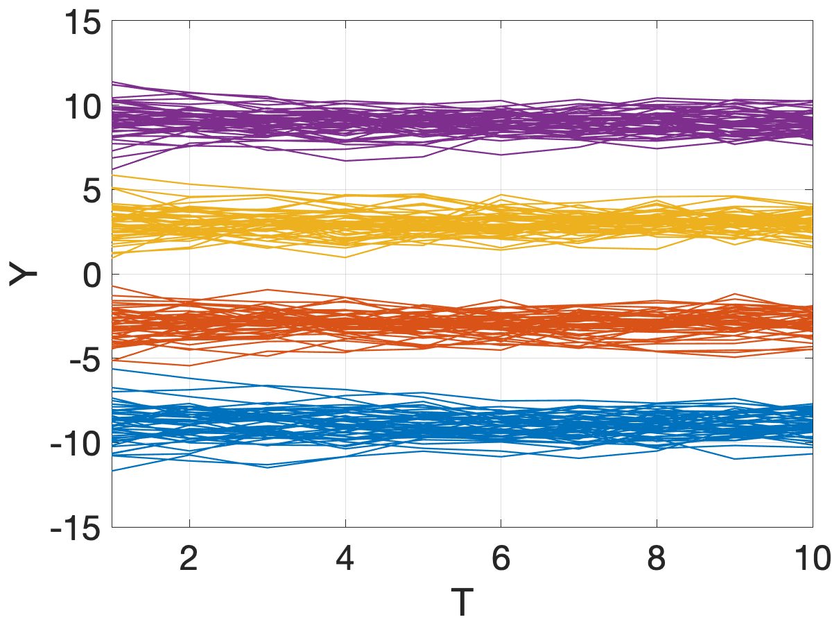
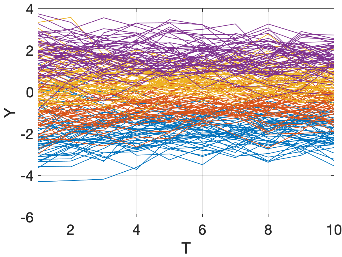
E.1.2 Details of the Simple DGPs
We start with the mean of . Assume the values of for group take the form of , where is a shifting constant and is a scaling constant. With loss of generality, we fix the mean of to 0,
| (E.2) |
It immediately follows that and
| (E.3) |
Next, is the only unknown coefficient in the DGP. To find a reasonable value for , we connect it to the variance of . As are assume to be identical within a group, the sample variance of is given by
Plugging in the expression of in (E.3), we have
| (E.4) |
To make the DGPs more comparable as more groups are considered, we assume is monotonically increasing in , e.g., for some constant . As a result, we can deduct the value of from (E.4),
| (E.5) |
It is straightforward to find controls the dispersion of the underlying DGP. A larger indicate are more separated and hence the group pattern become sharper, and vice versa.
E.1.3 General DGPs
The general DGP is based on the dynamic panel data model specified in (2.1) with an exogenous predictor that has common effect for all units. This DGP incorporates group heterogeneity in the fixed-effects, the lagged term and an exogenous predictor , as well as error variance .
DGP 3:
| (E.6) |
where , , and . For each , the initial value is specified to guarantee that the time series is strictly stationary. We assume there are balanced groups, with the true grouped coefficients summarized in Table (E.1). The AR(1) coefficients represent different degree of persistence persistence. The exogenous variable is drawn from and is drawn from , capped by 10.
| (FE) | (lagged) | (exo var.) | (variance) | |
| Group 1 | -0.15 | 0.4 | 0.16 | 0.500 |
| Group 2 | -0.05 | 0.8 | 0.14 | 0.375 |
| Group 3 | 0.05 | 0.5 | 0.12 | 0.250 |
| Group 4 | 0.15 | 0.7 | 0.10 | 0.125 |
E.2 Construction of Soft Pairwise Constraints
Number of constraints: We set the number of constraints and as a function of and to facilitate performance comparisons across different settings and to ensure that the information of constraints does not vanish as increases. Specifically, and are a predetermined proportion of the total number of correct constraints for each type which are given by,
| (E.7) | ||||
| (E.8) |
In the setting with , we have and . We choose randomly select 5% of these constraints, leading to and .
Type of pairwise constraints: The pairwise constraints are generated randomly. Given the number of PL constraints , each PL constraint is generated by randomly selecting a group and uniformly selecting two units within that group to be positive-linked. Similarly, for each of NL constraints, two unique groups are chosen at random and one unit is randomly selected from each. Regarding the remaining unselected units, we assume they are not restricted and have no prior belief on them.
Accuracy of pairwise constraints: Each constraint is annotated with a level of accuracy generating from a transformed Beta distribution defined on . We begin by drawing from a Beta distribution: if the constraint is correct, for some ; otherwise, . Then the level of confidence is so that its domain is . We derive in this manner to reflect the assumption that an expert should have less certainty in erroneous constraints than in correct ones.
Perturbation in pairwise constraints: To examine the performance with soft constraints under inaccurate prior belief, we artificially add errors to the randomly generated constraints. A fraction of the constraints are mislabeled – a positive-link would be mislabeled as a negative-link and vice versa. We turn true PL into NL and true NL into PL with .
All DGPs are equipped with the same set of pairwise constraints, e.g., we only draw pairwise constraints and construct weights once.
E.3 Alternative Estimators
We explore various types of estimators that differ in the prior belief on .
-
(i)
BGFE: The baseline Bayesian grouped fixed-effects (BGFE) estimator are correctly-specified, i.e. assuming that the true model exhibits time-invariant grouped heterogeneity and that variance of error term is constant (varying) across units in the simple (general) DGPs. No prior belief on is available for this estimator.
-
(ii)
BGFE-cstr: The baseline BGFE estimator that takes pairwise constraints into consideration.
-
(iii)
BGFE-oracle: This estimator is a variant of the BGFE estimator equipped with known true G.
We also evaluate the other Bayesian estimators with different prior assumptions on that don’t model group structure.
-
(iv)
Pooled: Bayesian pooled estimator views as a common parameter and, consequently, all units have the same prior level of .
-
(v)
Flat: flat-prior estimator assumes . There is no pooling across units in this case and ’s are individually estimated using their own history. This also amounts to sampling from a posterior whose mode is the MLE estimate.
E.4 Posterior Predictive Densities and Performance Evaluation
E.4.1 Posterior Predictive Densities
Given posterior draws, the posterior predictive distribution estimated from the MCMC draws is
| (E.9) |
We can therefore draw samples from by simulating (2.1) forward conditional on the posterior draws of and observations.
E.4.2 Point Forecasts
The optimal posterior forecast under quadratic loss function is obtain by minimizing the posterior risk, with is the posterior mean. Conditional on posterior draws of parameters, the mean forecast can be approximated by the Monte Carlo averaging,
| (E.10) |
and the RMSFE across units is given by
| (E.11) |
E.4.3 Set Forecasts
We construct set forecasts from the posterior predictive distribution of each unit. In particular, we adopt a Bayesian approach and report the highest posterior density interval (HPDI), which is the narrowest connected interval with coverage probability of . In other words, it requires that the probability of conditional on having observed the history be at least , i.e.,
| (E.12) |
and this interval is the shortest among all possible single connected candidate sets. Let be the lower bound and be the upper bound, then .
The assessment of set forecasts in simulation studies and empirical applications is based on two metrics: (1) the cross-sectional coverage frequency,
| (E.13) |
and (2) the average length of the sets ,
| (E.14) |
E.4.4 Density Forecasts
To compare the performance of density forecasts for various estimators, we examine the continuous ranked probability score (Matheson and Winkler, 1976; Hersbach, 2000) across units. The continuous ranked probability score (CRPS) is frequently used to assess the respective accuracy of two probabilistic forecasting models. It is a quadratic measure of the difference between the predictive cumulative distribution function, , and the empirical CDF of the observation with the formula as follows,
| (E.15) |
where is the realization at .
In practice, the true predictive cumulative distribution function or the PIT of is not available. We approximate it via the empirical distribution function for each unit based on the posterior draws from the predictive density,
| (E.16) |
Based on sorted posterior draws , we can calculate CRPS using the below representation by Laio and Tamea (2007),
| (E.17) |
Moreover, we report the average log predictive scores (LPS) to assess the performance of the density forecast from the view of the probability distribution function. As suggested in Geweke and Amisano (2010), the LPS for a panel reads as,
| (E.18) |
where the expectation can be approximated using posterior draws,
| (E.19) |
E.5 Simulation Results
E.5.1 Simple Dynamics Panel Data
To evaluate the advantage of pooling units into groups, we report the RMSE, bias, standard deviation, average length of 95% credible set, and frequentist coverage of the posterior estimate of across Monte Carlo repetitions. For the fixed effects , we only present the average bias as it may not be of importance for most empirical study.
The comparison across alternative estimators is shown in Table E.2. In DGP 1,the BGFE-cstr and BGFE estimators are equally accurate as the oracle estimator. This is not surprising because the units are well-separated by design, and the data provide sufficient information for the BGFE estimator to determine the group pattern. In this situation, prior knowledge of or the true group indices has quite marginal influence. The pooled estimator, on the other hand, erroneously pools all groups together, resulting in inaccurate estimates of and . Despite the fact that the flat estimator treats units separately, it is still inferior to the BGFE-type estimators. This is because it cannot utilize cross-sectional information to estimates parameters in this short panel and hence bears much larger bias.
In DGP 2, where the group pattern is less apparent, the BGFE-cstr estimator is arguably the most accurate. In contrast to the standard BGFE estimator, it uses cross-sectional data and pairwise constraints to determine the group pattern. These properties substantially reduce the biases of and , enabling the BGFE-cstr estimator to outperform the unconstrained estimator by a significant margin and to perform comparable to the oracle estimator. Remember that we manually add 20% incorrect constraints into the prior knowledge. Despite the presence of these misspecified constraints, the BGFE-cstr estimator is still able to extract relevant information from constraints in order to enhance the overall performance. The BGFE estimator, however, is unable to correctly reconstruct the group structure due to the noisy data, which results in the algorithm improperly grouping the units and hence generating inaccurate estimates.
| Group | ||||||||
| RMSE | Bias | Std | AvgL | Cov | Bias | Avg K | ||
| DGP 1 | BGFE-oracle | 0.0104 | 0.0037 | 0.0072 | 0.0276 | 0.92 | 0.0371 | 4 |
| BGFE-cstr | 0.0102 | 0.0030 | 0.0072 | 0.0282 | 0.94 | 0.0369 | 4.92 | |
| BGFE | 0.0103 | 0.0037 | 0.0071 | 0.0274 | 0.92 | 0.0377 | 4.4 | |
| Pooled | 0.3543 | 0.3543 | 0.0032 | 0.0125 | 0 | 1.7889 | - | |
| Flat | 0.1713 | 0.1711 | 0.0073 | 0.0283 | 0 | 0.8668 | - | |
| DGP 2 | BGFE-oracle | 0.0186 | 0.0030 | 0.0137 | 0.0527 | 0.95 | 0.0235 | 4 |
| BGFE-cstr | 0.0202 | 0.0058 | 0.0143 | 0.0557 | 0.93 | 0.0373 | 5.06 | |
| BGFE | 0.0546 | 0.0443 | 0.0212 | 0.0809 | 0.66 | 0.1357 | 4.78 | |
| Pooled | 0.2920 | 0.2919 | 0.0077 | 0.0298 | 0 | 0.5060 | - | |
| Flat | 0.1170 | 0.0834 | 0.0131 | 0.0509 | 0.14 | 0.2344 | - | |
Table E.3 provides a summary of the prediction performance of each estimator. In general, the conclusions of the one-step-ahead forecast agree with those of the estimation. In DGP 1, the performance of the three BGFE estimators are quite similar, followed by the flat and pooled estimators. In DGP 2, the BGFE-cstr estimator, which utilizes prior belief on , beats the other feasible estimators in point, set, and density forecast and is comparable to the oracle estimator.
| Point Forecast | Set Forecast | Density Forecast | ||||||
| RMSFE | Error | Std | AvgL | Cov | LPS | CRPS | ||
| DGP 1 | BGFE-oracle | 0.4989 | 0.0001 | 0.4989 | 1.9627 | 0.95 | 0.7254 | 0.2818 |
| BGFE-cstr | 0.4991 | 0.0004 | 0.4990 | 1.9666 | 0.95 | 0.7256 | 0.2819 | |
| BGFE | 0.4990 | 0.0001 | 0.4990 | 1.9616 | 0.95 | 0.7255 | 0.2818 | |
| Pooled | 0.6401 | 0.0006 | 0.6404 | 3.0114 | 0.98 | 1.0064 | 0.3657 | |
| Flat | 0.5620 | 0.0003 | 0.5622 | 2.4265 | 0.97 | 0.8544 | 0.3184 | |
| DGP 2 | BGFE-oracle | 0.4990 | 0.0001 | 0.4989 | 1.9629 | 0.95 | 0.7254 | 0.2819 |
| BGFE-cstr | 0.5021 | 0.0001 | 0.5021 | 1.9790 | 0.95 | 0.7314 | 0.2836 | |
| BGFE | 0.5186 | 0.0002 | 0.5187 | 2.0546 | 0.95 | 0.7633 | 0.2930 | |
| Pooled | 0.5396 | 0.0005 | 0.5395 | 2.2444 | 0.96 | 0.8079 | 0.3052 | |
| Flat | 0.5286 | 0.0002 | 0.5287 | 2.1165 | 0.95 | 0.7841 | 0.2987 | |
E.5.2 General Panel Data
As the number of parameters increases for DGP 3, we present the RMSE and absolute bias of and , as well as metrics for point and density prediction. In addition, all BGFE estimators now account for heteroskedasticity because the cross-sectional variance in DGP 3 is informative to group structure. As a result, we have the BGFE-he-oracle, BGFE-he-cstr and BGFE-he estimators in this exercise, where ”he” denotes heteroskedasticity. For comparison, we also offer the BGFE-ho-cstr estimator, which assumes homoskedasticity, and Flat-he estimator, which is the heteroskedastic flat estimator.
| Estimates | Forecast | Group | ||||||||||
| RMSFE | LPS | AvgK | PctK | |||||||||
| Flat-he | 0.258 | 0.199 | 0.131 | 0.098 | 0.200 | 0.149 | 0.026 | 0.014 | 0.667 | 1.108 | - | - |
| BGFE-he-oracle | 0.126 | 0.137 | 0.092 | 0.101 | 0.119 | 0.132 | 0.569 | 0.602 | 0.840 | 0.706 | 4 | 1 |
| BGFE-he-cstr | 0.171 | 0.164 | 0.290 | 0.179 | 0.125 | 0.135 | 0.566 | 0.608 | 0.847 | 0.716 | 4.087 | 0.914 |
| BGFE-ho-cstr | 0.218 | 0.198 | 0.328 | 0.220 | 0.140 | 0.144 | 0.625 | 0.671 | 0.850 | 0.769 | 4.342 | 0.682 |
| BGFE-he | 0.303 | 0.317 | 0.560 | 0.482 | 0.137 | 0.147 | 0.601 | 0.640 | 0.871 | 0.756 | 3.575 | 0.534 |
| Pooled | 0.444 | 0.503 | 1.262 | 1.527 | 0.131 | 0.148 | 0.734 | 0.805 | 0.993 | 0.910 | - | - |
Notes: The first line gives the levels of the each metrics based on the Flat-he estimator, which is the benchmark model, and the following lines in the columns head ”Estimates” and ”Forecast” present ratios of the respective method relative those based on the flat-he estimator. In the columns head ”Group”, we show the average of number of groups (AvgK) and the percentage of iterations that the posterior sampler selects (PctK) averaged over 1,000 runs of algorithm. is RMSE of the posterior mean estimator. is the absolute bias of the posterior mean estimator.
Table E.4 presents the relative performance of estimation and forecasting for DGP 3. The benchmark model is Flat-he. Several findings arise. First, the gain from incorporating pairwise constraints is evident. It reduces the RMSE and bias for all parameters and improve both point and density forecast, when comparing BGFE-he-cstr to BGFE-he. The percentage of the Gibbs sampler that visits the true number of groups grows considerably from 53.4% to 91.4%. Even when pairwise constraints are taken into account, this percentage is just 68.2% if heteroskedasticity is ignored. Second, when we include prior belief on , the improvement in , the AR coefficient, is the greatest among all three grouped coefficients with a bias reduction of more than 60%. This also suggests that the AR coefficient may be more sensitive to the estimated group structure. Thirdly, BGFE-he-cstr and BGFE-ho-cstr have comparable RMSFE values, but BGFE-he-cstr has a significantly lower LPS, showing that modeling heteroskedasticity in the current setting is favorable for the density forecast. The empirical results below also confirm this finding. Lastly, all BGFE-type estimators generate similar estimates for the exogenous variables that don’t have group effects on as the improvement in and are marginal when prior belief on group is included or when true group is imposed.
E.5.3 Computational Time
We compare the running times of each estimator using the simulation with the general DGPs. For each estimator, we run the block Gibbs samplers with 5,000 iterations after a burn-in of 5,000 draws. We calculate the running time by averaging over 1,000 repetitions. All programs, including this exercise, the simulations above, and the empirical analysis in Section 4 were executed in Matlab 2020a running on a server with Intel Skylake CPUs and 32 GB of RAM.
Table E.5 shows the running time in seconds. It suggests that modeling group structure does not considerably increase computational load. The running time of the BGFE-he estimator is comparable to that of the Flat estimator when the number of observations is small. As increases, the BGFE-he estimators take slightly more time to finish than the flat estimator. The BGFE-he-cstr estimator requires approximately 20% more time to complete the calculations than the BGFE-he estimator. This is because BGFE-he-cstr adapts pairwise constraints and has additional term to evaluate in the posterior distribution of the group indices. Notice that we fix the scaling constant in this experiment. If we find the optimal using grid search as proposed in Section 4.1.2, the running time of BGFE-he-cstr will be times as great as what is shown below, where is the size of the grid.
| N | T | BGFE-he-cstr | BGFE-he | Flat | Pooled |
| 100 | 5 | 74.9 | 62.1 | 1.2 | 61.7 |
| 10 | 82.5 | 69.8 | 1.3 | 64.7 | |
| 20 | 86.1 | 75.7 | 1.3 | 62.4 | |
| 200 | 5 | 145.0 | 111.9 | 1.2 | 114.3 |
| 10 | 146.2 | 118.8 | 1.3 | 113.0 | |
| 20 | 159.4 | 133.2 | 1.5 | 117.0 |
It is possible to speed the algorithm up especially when we select the optimal value for . Wang and Dunson (2011) propose the sequential updating and greedy search (SUGS) algorithm, which essentially simplifies the algorithm 1 with approximation. The SUGS algorithm allows fast yet accurate approximate Bayes inferences under DP priors with just a single cycle of simple calculations for each unit, while also producing marginal likelihood estimates to be used in selecting the constant . This will be left for future study.
Appendix F Data Description
F.1 Inflation of the U.S. CPI Sub-Indices
The seasonally adjusted series of CPI for All Urban Consumers (CPI-U) for subcategories at all display level are obtained from the BLS Online Databases.212121https://data.bls.gov/PDQWeb/cu The raw data contains 318 series, which are recorded on a monthly basis and spanned the period from January 1947 to August 2022. Notice that the raw dataset doesn’t include an indicator for the expenditure categories. We manually merge the raw dataset with the table of content of CPI entry level items222222https://www.bls.gov/cpi/additional-resources/entry-level-item-descriptions.xlsx by entry level item (ELI) code, the series description, and universal classification codes (UCC), if necessary.232323Some series are labeled by UCC rather than ELI. The concordance provided by the BLS can be found here: https://www.bls.gov/cpi/additional-resources/ce-cpi-concordance.htm.
Series can enter and exit the sample. The BLS discontinued and launched series on a regular basis owing to changes in source data and methodology, for example, see the Post for the updates on series since 2017. The measure of certain subcategories was impacted by the Pandemic and hence missing. Since the Pandemic, the related activities and venues (sports events, bars, schools) were canceled and close temporarily, such as admission to sporting events (SS62032), distilled spirits away from home (SS20053), food at elementary and secondary schools (SSFV031A), etc. We chose to not impute the missing values since there was no clear benchmark to compare with, especially given the depressed economic conditions.
The CPI-U consists of eight major expenditure categories (1) Apparel; (2) Education and Communication; (3) Food and beverages; (4) Housing; (5) Medical Care; (6) Recreation; (7) Transportation; (8) Other goods and services. Each major category contains multiple subcategories, resulting in a hierarchy of categories with increasing specificity. BLS provides a detailed table242424 https://download.bls.gov/pub/time.series/cu/cu.item. that records the series code, series name, and display level. We resort to the display level to build the tree structure of the CPI sub-indices and eliminate those parent nodes, as illustrated in Figure F.1.
forked edges,
for tree=
grow = east,
align = center,
font=,
[All Items
[Housing
[Shelter
[Rent of primary residence]
[Owners’ equivalent rent of residences]
]
[Fuels and utilities
[Water sewer and trash]
[Household energy
[Fuel oil and other fuels
[Fuel oil]
[Propane kerosene and firewood]]
[Energy services
[Electricity]
[Utility gas service]]]
]
]
[Transportation
[…]
]
[Food and beverages
[…]
]
]
Because all CPI data is available on a monthly basis, we use the unemployment gap as labor market slack measures in the Phillips curve model. We use the seasonally adjusted unemployment rate252525https://fred.stlouisfed.org/series/UNRATE from FRED and construct the “gap” measures using the Hamilton filter (Hamilton, 2018). The Hamilton filter has two parameters: number of lags and number of lookahead periods . We follow Hamilton’s suggestion and set and , or an AR(12) process, additionally lagged by 24 lookahead periods for the monthly time series.
F.2 Income and Democracy
All data in this section are taken from the replication files of BM.262626 https://www.dropbox.com/s/ssjabvc2hxa5791/Bonhomme_Manresa_codes.zip?dl=0 The data set contains a balanced panel of 89 countries and 7 periods at a five-year interval over 1970-2000. The main measure of democracy is the Freedom House Political Rights Index. A country receives the highest score if political rights come closest to the ideals suggested by a checklist of questions, beginning with whether there are free and fair elections, whether those who are elected rule, whether there are competitive parties or other political groupings, whether the opposition plays an important role and has actual power, and whether minority groups have reasonable self-government or can participate in the government through informal consensus. See more details in Acemoglu et al. (2008), Section 1.
Table F.1 contains descriptive statistics for the main variables. The sample period is 1970–2000, and each observation corresponds to five-year intervals. The table shows these statistics for all countries and also for high- and low-income countries, split according to the median of the countries’ averaged income. The comparison of high- and low-income countries in the medium and lower panels reveals the pattern that richer countries tend to be more democratic.
| Mean | Median | S.E. | Min | Max | |
| Full Sample | |||||
| Democracy index | 0.5535 | 0.5000 | 0.3727 | 0 | 1.0000 |
| GDP per capita (in log) | 8.2534 | 8.2444 | 1.0763 | 5.7739 | 10.4450 |
| High-Income | |||||
| Democracy index | 0.7852 | 1.0000 | 0.2934 | 0 | 1.0000 |
| GDP per capita (in log) | 9.1490 | 9.1975 | 0.6079 | 7.4970 | 10.4450 |
| Low-Income | |||||
| Democracy index | 0.3247 | 0.1667 | 0.2973 | 0 | 1.0000 |
| GDP per capita (in log) | 7.3576 | 7.3208 | 0.6051 | 5.7739 | 8.81969 |
Appendix G Additional Empirical Results
G.1 Inflation of the U.S. CPI Sub-Indices
Figure G.1 shows the posterior mean of the number of active groups (red) along with total number of available CPI sub-indices (dark blue). Note that we choose not to show the credible set or the distribution of because the distributions are concentrated around a single number in most samples.
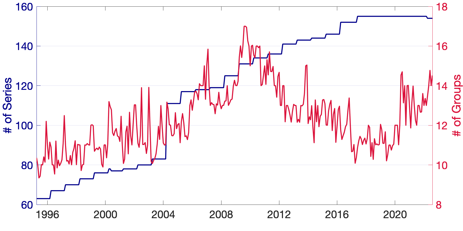
Figure G.2 shows the selected scaling constant over time.
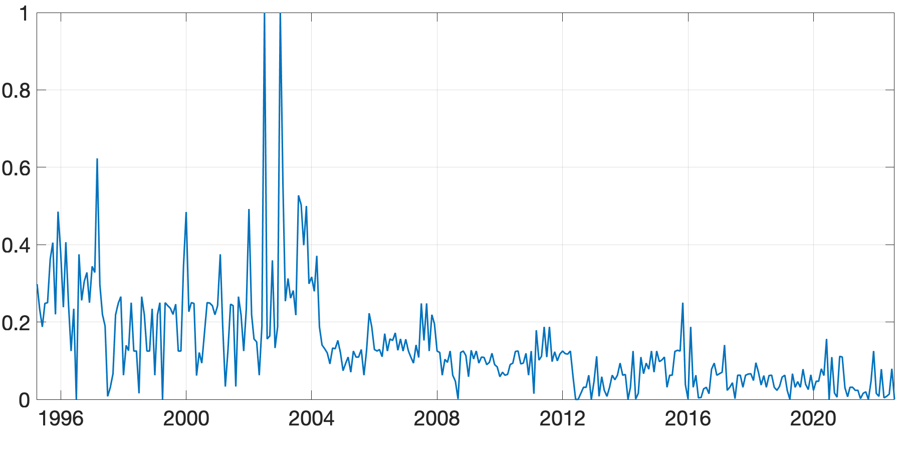
Table G.1 and G.2 present the ratio of RMSE between each estimator and AR-he for each expenditure category in five periods: 1995-1999, 2000-2004, 2005-2009, 2010-2014, 2015-2019, 2020-2022. Similar results for the difference of LPS are shown in Table G.3 and G.4.
| Full | 95 - 99 | 00 - 04 | 05 - 09 | 10 - 14 | 15 - 19 | 20 - 22 | |
| Average of All Series | |||||||
| BGFE-he-cstr | |||||||
| BGFE-he | |||||||
| BGFE-ho | |||||||
| AR-he-PC | |||||||
| Pooled | |||||||
| Category 1: Apparel | |||||||
| BGFE-he-cstr | |||||||
| BGFE-he | |||||||
| BGFE-ho | |||||||
| AR-he-PC | |||||||
| Pooled | |||||||
| Category 2: Education and Communication | |||||||
| BGFE-he-cstr | |||||||
| BGFE-he | |||||||
| BGFE-ho | |||||||
| AR-he-PC | |||||||
| Pooled | |||||||
| Category 3: Food and Beverages | |||||||
| BGFE-he-cstr | |||||||
| BGFE-he | |||||||
| BGFE-ho | |||||||
| AR-he-PC | |||||||
| Pooled | |||||||
| Category 4: Housing | |||||||
| BGFE-he-cstr | |||||||
| BGFE-he | |||||||
| BGFE-ho | |||||||
| AR-he-PC | |||||||
| Pooled | |||||||
Notes: Benchmark model = AR-he.
| Full | 95 - 99 | 00 - 04 | 05 - 09 | 10 - 14 | 15 - 19 | 20 - 22 | |
| Category 5: Medical Care | |||||||
| BGFE-he-cstr | |||||||
| BGFE-he | |||||||
| BGFE-ho | |||||||
| AR-he-PC | |||||||
| Pooled | |||||||
| Category 6: Recreation | |||||||
| BGFE-he-cstr | |||||||
| BGFE-he | |||||||
| BGFE-ho | |||||||
| AR-he-PC | |||||||
| Pooled | |||||||
| Category 7: Transportation | |||||||
| BGFE-he-cstr | |||||||
| BGFE-he | |||||||
| BGFE-ho | |||||||
| AR-he-PC | |||||||
| Pooled | |||||||
| Category 8: Other Goods and Services | |||||||
| BGFE-he-cstr | |||||||
| BGFE-he | |||||||
| BGFE-ho | |||||||
| AR-he-PC | |||||||
| Pooled | |||||||
Notes: Benchmark model = AR-he.
| Full | 95 - 99 | 00 - 04 | 05 - 09 | 10 - 14 | 15 - 19 | 20 - 22 | |
| Average of All Series | |||||||
| BGFE-he-cstr | |||||||
| BGFE-he | |||||||
| BGFE-ho | |||||||
| AR-he-PC | |||||||
| Pooled OLS | |||||||
| Category 1: Apparel | |||||||
| BGFE-he-cstr | |||||||
| BGFE-he | |||||||
| BGFE-ho | |||||||
| AR-he-PC | |||||||
| Pooled | |||||||
| Category 2: Education and Communication | |||||||
| BGFE-he-cstr | |||||||
| BGFE-he | |||||||
| BGFE-ho | |||||||
| AR-he-PC | |||||||
| Pooled | |||||||
| Category 3: Food and Beverages | |||||||
| BGFE-he-cstr | |||||||
| BGFE-he | |||||||
| BGFE-ho | |||||||
| AR-he-PC | |||||||
| Pooled | |||||||
| Category 4: Housing | |||||||
| BGFE-he-cstr | |||||||
| BGFE-he | |||||||
| BGFE-ho | |||||||
| AR-he-PC | |||||||
| Pooled | |||||||
Notes: Benchmark model = AR-he.
| Full | 95 - 99 | 00 - 04 | 05 - 09 | 10 - 14 | 15 - 19 | 20 - 22 | |
| Category 5: Medical Care | |||||||
| BGFE-he-cstr | |||||||
| BGFE-he | |||||||
| BGFE-ho | |||||||
| AR-he-PC | |||||||
| Pooled | |||||||
| Category 6: Recreation | |||||||
| BGFE-he-cstr | |||||||
| BGFE-he | |||||||
| BGFE-ho | |||||||
| AR-he-PC | |||||||
| Pooled | |||||||
| Category 7: Transportation | |||||||
| BGFE-he-cstr | |||||||
| BGFE-he | |||||||
| BGFE-ho | |||||||
| AR-he-PC | |||||||
| Pooled | |||||||
| Category 8: Other Goods and Services | |||||||
| BGFE-he-cstr | |||||||
| BGFE-he | |||||||
| BGFE-ho | |||||||
| AR-he-PC | |||||||
| Pooled | |||||||
Notes: Benchmark model = AR-he.
G.1.1 Network Visualization of Posterior Similarity Matrix
In our empirical work, we estimate the posterior similarity matrix (PSM) among 154 series for the last sample (August 2022). Presenting and examining estimates pairwise posterior probabilities in PSM would be thoroughly uninformative. Hence we characterize the estimated PSM graphically as network graphs, which contain node names, node color, and link size (one per link since the network is undirected).
-
•
Node name shows the item names of CPI sub-indices.
-
•
Node color indicates the group structure used in the prior, e.g, expenditure category.
-
•
Link size represents the pairwise probabilities in the PSM.
We use the qgraph package in R for network visualization. Node locations are determined by a modified version of a force-embedded algorithm proposed by Fruchterman and Reingold (1991). Figure G.3 show the full-sample CPI sub-index network graphs.
See graphs/app_CPI_details/fcst_nlag3_window48_hetsk_NKPC_final_2022sep/fig_network_name.pdf
G.1.2 Heteroskedasticity vs. Homoskedasticity
We conclude by examining how grouped heteroskedasticity impacts forecast accuracy and why this is important. For illustrative purposes, we focus on the two BGFE estimators, BGFE-he and BGFE-ho, that do not involve pairwise constraints.
A distinguishing characteristic between BGFE-he and BGFE-ho is the estimated number of groups. Figure G.4 depicts the number of groups over samples. BGFE-he estimator forms 9 groups for the beginning of the sample, and increase it during the Great Recession and the Pandemic. However, the estimated number of groups for BGFE-ho is rather low in the 1990s, and progressively increases to around seven by the end of the sample. It is noticeable that when heteroskedasticity is allowed, there are more groups than when it is not. This is intuitive. Two groups can be expected to have comparable estimates of grouped fixed-effects and slope coefficients, but vastly different error variances. As a result, allowing for heteroskedasticity would result in a more refined group structure and increase the overall number of groups.
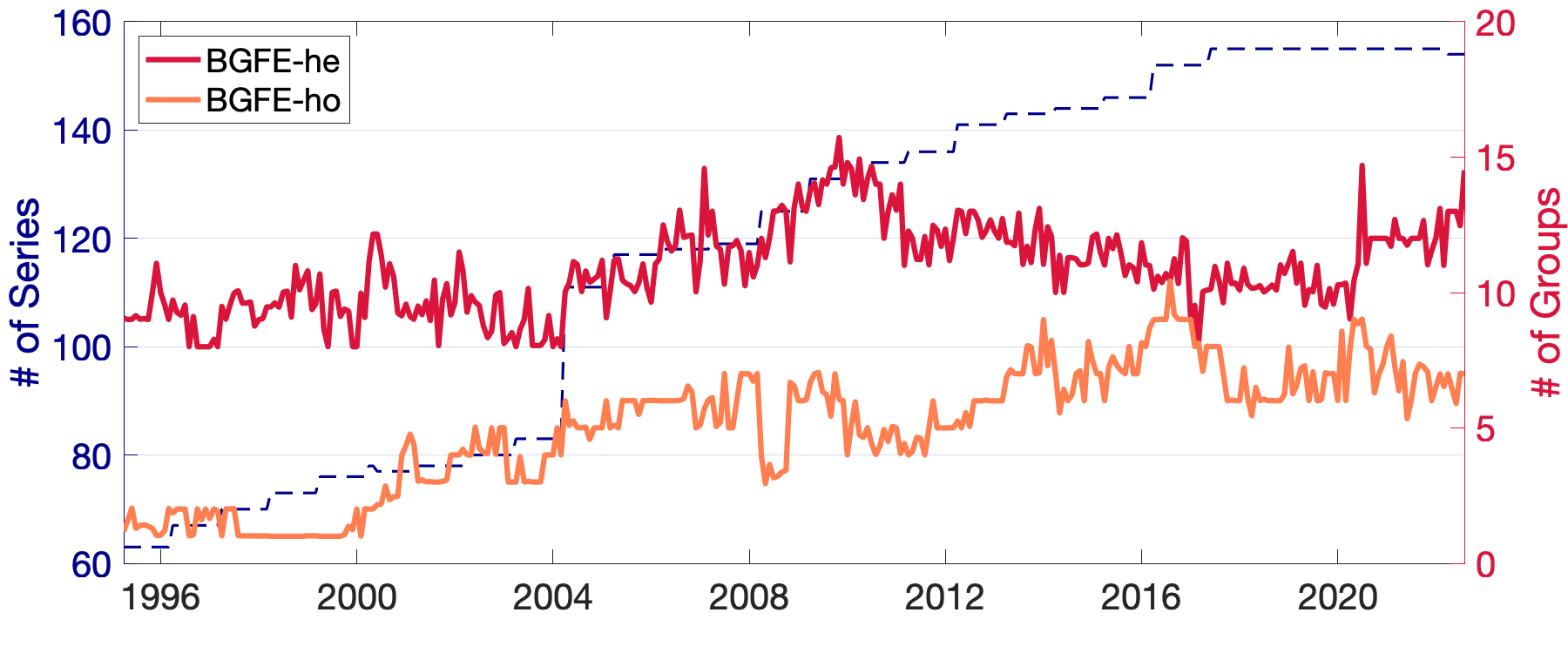
As seen in Figure 6 and 7, the grouped heteroskedasticity doesn’t improve the point forecast but the density forecast. Figure G.5 depicts a clear perspective of it and demonstrates the performance of point and density forecasts through time. In panel (a), we observe that the ratio of RMSE is generally around one over the whole sample, meaning that heteroskedasticity cannot improve the point forecast in general. In panel (b), the difference in LPS is consistently negative. This demonstrates that the improved density prediction performance is not a fluke and that enabling heteroskedasticity improves the density forecast regardless of sample. This is actually in line with the simulation results presented in Table E.4.
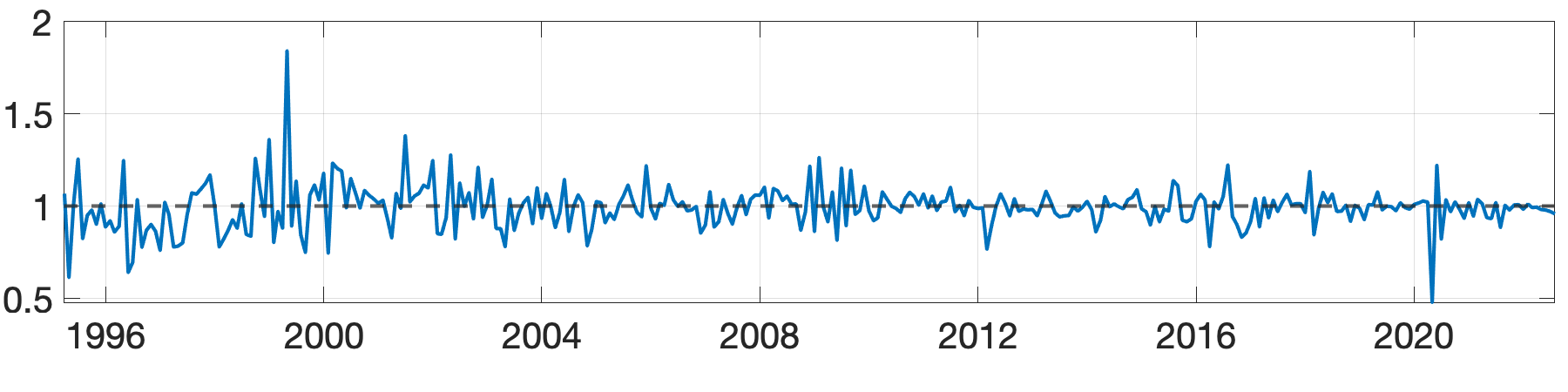
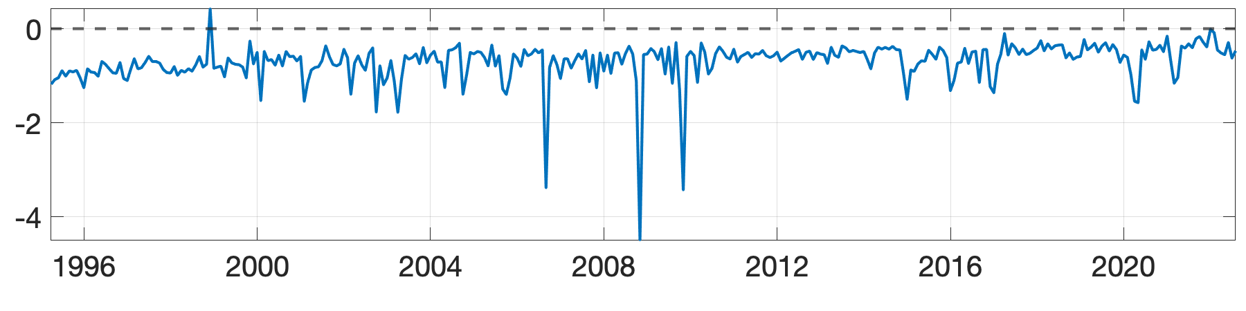
Density forecasts vary substantially across categories. We pick three typical sub-categories and plot their posterior predictive densities of August 2022 in Figure G.6. The vertical dashed black lines represent the actual values. Several insights emerge while comparing these three subcategories. First, BGFE-he and BGFE-ho provide comparable posterior means for all three subcategories - the posterior predictive densities concentrate around the similar price levels. This explains why BGFE-he and BGFE-ho have comparable results in point forecasting. Second, BGFE-he reveals different predictive variance. As the rolling sample size is set to 4 years, all observations throughout the Pandemic are included, and it is anticipated that the price levels of elementary and high school (basic education) tuition and fees, major appliances, and airline prices would respond differently to the shock. Intuitively, education tuition and fees should not fluctuate as much as other prices, while airline fares have been strongly influenced by the fluctuating oil prices since the beginning of the Pandemic. Consequently, accounting for heteroskedasticity successfully captures this characteristic, such that college tuition and fees have a smaller predictive variance than that of BGFE-ho, but airline fares have a greater predictive variance.
Combing these two observations together reveals why BGFE-he has a better density forecast: the capacity to optimally cluster units according to the error variance and accommodate heteroskedasticity. For elementary and high tuition and fees, providing that both BGFE-he and BGFE-ho yields accurate posterior mean, BGFE-he yields much lower predictive variance, decreasing the LPS dramatically. Both BGFE-he and BGFE-ho underestimate the inflation rate for airline fares, but BGFE-he subtly creates a greater predicted variance to account for the wild probable shift in this sub-category and hence reduces the LPS significantly. Major appliances is an example to show that BGFE-he and BGFE-ho generate comparable density forecasts for some sub-categories.
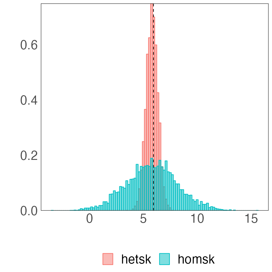
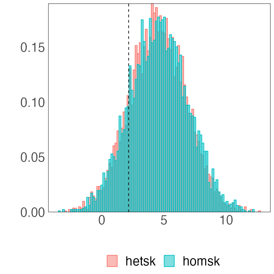
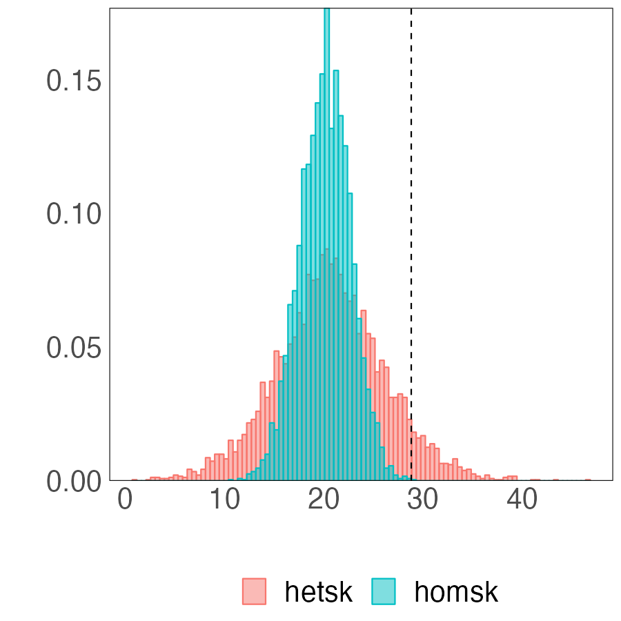
G.2 Income and Democracy
G.2.1 Results of Specification 1
We start our analysis with the specification 1 in (4.15). Table G.5 demonstrates the posterior probability of the number of groups utilizing various estimators. Notably, the BGFE-ho in this specification is identical to the primary model in BM, allowing us to evaluate the optimal number of groups. BGFE-ho creates 8 groups in all posterior draws, which is consistent with BM’s conclusion of using BIC: the upper bound of the true number of groups is 10. Despite the fact that BM is unable to validate the ideal number of groups for their study, our BGFE-ho estimator provides an accurate estimate of it. Intriguingly, accounting for heteroskedasticity drastically reduces the number of groups, with BGFE-he identifying three groups in 92.9% of posterior draws. Adding pairwise constraints based on geographic information increase the number groups. Two-third of posterior draws from BGFE-he-cstr generate 5 group.
| BGFE-he-cstr | BGFE-he | BGFE-ho | |
| 0.000 | 0.000 | 0.000 | |
| 0.000 | 0.929 | 0.000 | |
| 0.344 | 0.071 | 0.000 | |
| 0.656 | 0.000 | 0.000 | |
| 0.000 | 0.000 | 1.000 |
The marginal data density (MDD) of each estimators in Table G.6 provides some insight on different models. Even while BGFE-ho produces eight groups and has a tendency to overfit, its MDD is the lowest of the three estimators. BGFE-he with fewer groups is superior to BGFE-ho with higher MDD. BGFE-he-cstr has the highest MDD because the pairwise constraints give direction on grouping and identify the ideal group structure, which BGFE-he cannot uncover without our prior knowledge.
| BGFE-he-cstr | BGFE-he | BGFE-ho |
| 425.690 | 381.218 | 368.918 |
We focus on the BGFE-he-cstr estimator and use the approach outlined in Section 3.2 to identify the unique group partitioning . The left panel of Figure G.7 presents the world map colored by , while the right panel present the group-specific averages of democracy index over time. The estimated group structure features four distinct groups, which is coincident to the choice of BM. As described in BM, we refer to groups 1-4 as the “high-democracy”, “low-democracy”, “early transition”, and “late transition” group, respectively. With the exception of the “early transition” group that is slight at odd with the counterpart in BM, the group-specific averages of the democracy index for all other groups are relatively similar to those in BM. Notice that BM manually sets the number of groups to four, but we discover that four is the optimal number. Consequently, by employing model specification 1 and accounting for heteroskedasticity, we find the support for BM’s main results.
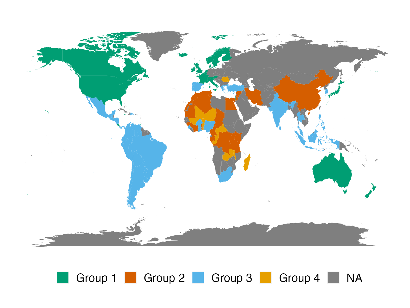
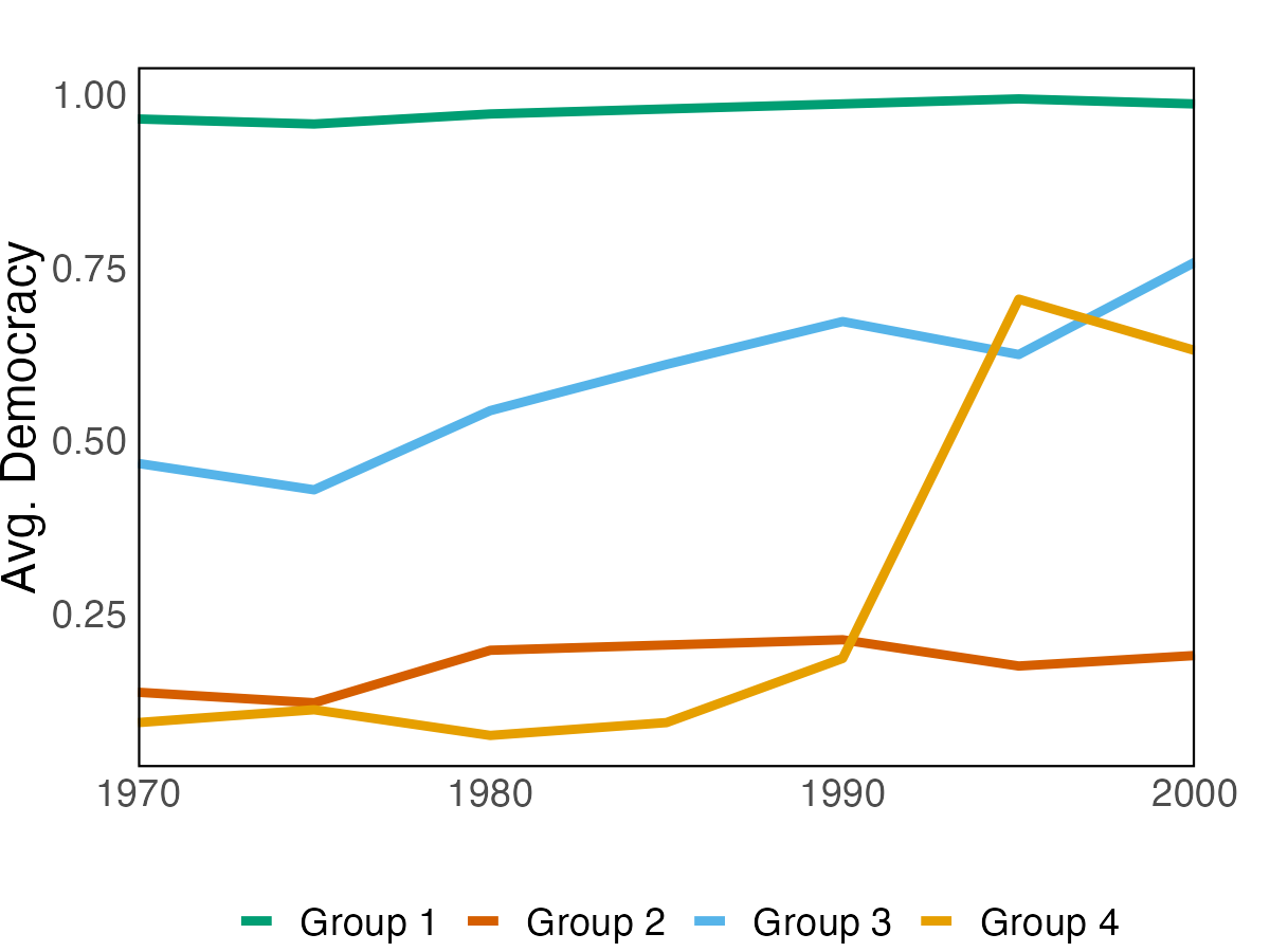
Table G.7 shows the posterior mean and 90% credible set for each coefficient, with fixing at the point estimate . Comparing to the pooled OLS, and once we incorporate the group-specific time patterns. The results are essentially consistent with the conclusion in BM: there is modest persistence and a positive effect of income on democracy, but the cumulative income effect is quantitatively small.
| Lagged democracy () | Lagged Income () | |||
| Coef. | Cred. Set | Coef. | Cred. Set | |
| BGFE-he-cstr | 0.499 | [0.438, 0.558] | 0.040 | [0.027, 0.053] |
| Pooled OLS | 0.665 | [0.616, 0.718] | 0.082 | [0.065, 0.100] |
G.2.2 Network Visualization of Posterior Similarity Matrix
Figure G.8 and G.9 show the full-sample country network graphs, for specification 1 and 2 respectively. Node color reflects the geographic information used to construct the group structure in the prior.