Incrementally Stochastic and Accelerated Gradient Information mixed Optimization for Manipulator Motion Planning
Abstract
This paper introduces a novel motion planner, incrementally stochastic and accelerated gradient information mixed optimization (iSAGO), for robotic manipulators in a narrow workspace. Primarily, we propose the overall scheme of iSAGO informed by the mixed momenta for an efficient constrained optimization based on the penalty method. In the stochastic part, we generate the adaptive stochastic momenta via the random selection of sub-functionals based on the adaptive momentum (Adam) method to solve the body-obstacle stuck case. Due to the slow convergence of the stochastic part, we integrate the accelerated gradient descent (AGD) to improve the planning efficiency. Moreover, we adopt the Bayesian tree inference (BTI) to transform the whole trajectory optimization (SAGO) into an incremental sub-trajectory optimization (iSAGO), which improves the computation efficiency and success rate further. Finally, we tune the key parameters and benchmark iSAGO against the other 5 planners on LBR-iiwa on a bookshelf and AUBO-i5 on a storage shelf. The result shows the highest success rate and moderate solving efficiency of iSAGO.
Index Terms:
Constrained Motion Planning, Collision Avoidance, Manipulation PlanningI INTRODUCTION
The industrial manufactory has widely applied robots in various areas such as welding and product loading or placing. Most of them always execute the above tasks under manual teaching or programming. So automatic production urges an efficient and robust optimal motion planning (OMP) algorithm to elevate industrial intelligence.
Though former OMP studies gain a collision-free optimal trajectory for a safe and smooth motion by numerical optimization [1, 2, 3, 4] or probabilistic sampling [5, 6, 7, 8, 9, 10], there still exist two main concerns this paper aims to solve:
(i) Reliability: The numerical methods, such as CHOMP[1], GPMP[2], and TrajOpt[3], can rapidly converge to a minimum with descent steps informed by the deterministic momenta/gradients. However, the local minima (i.e., failure plannings) are unavoidable with an inappropriate initial point. That is because the momenta information only describes the manifold of a local space near the initial point. So it is difficult for them to plan a safe motion with a high success rate (i.e., high reliability) in a narrow space.
(ii) Efficiency: The sampling method like STOMP[8] directly samples the trajectories to gain the optima. Others like RRT-Connect [7] grow a searching tree by the randomly sampled waypoints. Their sampling and wiring process can generate safe trajectories free of manifold information. However, their efficiency highly depends on the proportion the feasible subspace takes of the overall searching space. So the indiscriminate process takes enormous computation resources (i.e., low efficiency) in a narrow space.
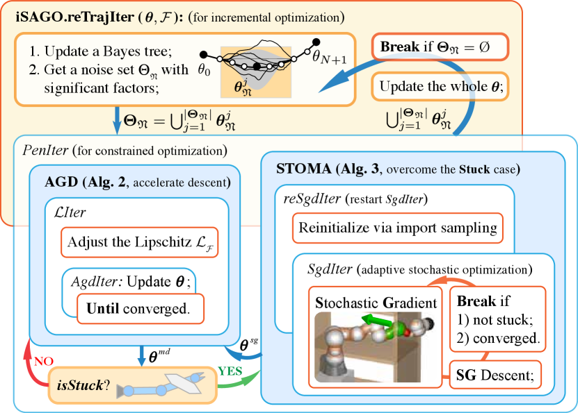
This paper proposes iSAGO (Figure 1), which integrates the Stochastic and Accelerated information of Gradients and builds a Bayes tree for an incremental Optimization:
(i) To address reliability, Stochastic trajectory optimization with moment adaptation (STOMA, Section IV-C) overcomes the local minima from the body-obstacle stuck cases by randomly selecting variables, such as collision-check balls, time intervals, and penalty factors. The information leakage of the stochastic momenta can somewhat modify OMP’s manifold with fewer local minima.
(ii) Considering the low efficiency of STOMA with convergence rate, iSAGO integrates accelerated gradient descent (AGD, Section IV-B) in the non-stuck case because its convergence rate of gradient norm is proven optimal in the first-order convex optimization. Furthermore, iSAGO adopts Bayes tree inference to optimize the trajectory incrementally (Section IV-A) for the further efficiency elevation, which optimizes the convex or non-convex sub-trajectories separately in iSAGO.reTrajOpt.
II RELATED WORKS
II-A Numerical Optimization
The main concern of numerical optimization is rapidly descending to an optimum. CHOMP [1], ITOMP [11], and GPMP [2] adopt the gradient descent method with the fixed step size. CHOMP uses Hamiltonian Monte Carlo (HMC) [12] for success rate improvement. To lower the computational cost, GPMP and dGPMP [4] adopt iSAM2 [13] to do incremental planning, and each sub-planning converges with a super-linear rate via Levenberg–Marquardt (LM) [14] algorithm. Meanwhile, ITOMP interleaves planning with task execution in a short-time period to adapt to the dynamic environment. Moreover, TrajOpt [3] uses the trust-region [15] method to improve efficiency. It is also adopted by GOMP [16] for grasp-optimized motion planning with multiple warm restarts learned from a deep neural network. Instead of deep learning, ISIMP [17] interleaves sampling and interior-point optimization for planning. Nevertheless, the above methods may converge to local minima when the objective function is not strongly convex.
AGD [18, 19] has recently been developed and implemented on the optimal control [20, 21] of a dynamic system described by differential equations whenever the objective is strongly convex or not. Moreover, stochastic optimization employs the momentum theorems of AGD and solves the large-scale semi-convex cases [22], which generates stochastic sub-gradient via the random sub-datasets selection. Adam [23] upgrades RMSProp [24] and introduces an exponential moving average (EMA) for momentum adaptation. Furthermore, [25] adopts Adam to overcome the disturbance of a UAV system.
II-B Probabilistic Sampling
Unlike the numerical method, the sampling method constructs a search graph to query feasible solutions or iteratively samples trajectories for motion planning.
PRM [5] and its asymptotically-optimal variants like PRM* [9] and RGGs [26] make a collision-free connection among the feasible vertexes to construct a roadmap. Then they construct an optimal trajectory via shortest path (SP) algorithms like Dijkstra [27] and Chehov [28], which store and query partial trajectories efficiently. Unlike PRM associated with SP, RRT [6] and its asymptotically-optimal variants like RRT* [9] and CODEs [10] find a feasible solution by growing rapidly-exploring random trees (RRTs).
III PROBLEM FORMULATION
III-A Objective functional
We adopt the probabilistic inference model of GPMP [2] to infer a collision-free optimal trajectory given an environment with obstacles, a manipulator’s arm, start, and goal.
III-A1 GP prior
Gaussian process (GP) describes a multi-variant Gaussian distribution of trajectory . and determine its expectation value and covariance matrix of trajectory , respectively, where a set denotes a period of time from to . Since the above distribution originates from Gauss–Markov model (GMM)111Section 4 of [2] introduces GP-prior, GMM generated by a linear time-varying stochastic differential equation (LTV-SDE), and GP-interpolation utilized by Section 5 for up-sampling. , informed by the start and goal under zero acceleration assumption, we define the smooth functional
| (1) |
III-A2 Collision avoidance
Since the collision-free trajectory means a safe motion or successful planning, we first utilize to map from a state at time to the position state of a collision-check ball (CCB-) on the manipulator. Then we calculate the collision cost , which increases when the distance between and its closest obstacle decreases, and define the obstacle functional
| (2) |
where consists of CCBs.
(i) Stuck case and local minima: The functional (2) consists of discrete CCBs for calculating the cost and gradient. So there may exist the sub-gradients with opposite directions in a narrow workspace. In this case, the gradient of (2) will approach zero when a collision cost is still high. It is a so-called body-obstacle stuck case that results in the local minima. According to Section IV-C1 and the objective functional (6), all local minima are unsafe trajectories because the non-convexity originates from the obstacle part (2) caused by the stuck case rather than the convex GP part (1).
(ii) Continuous-time safety: Though the above form combines the collision cost with the change rate of CCB state for the continuous-time collision avoidance between two adjacent waypoints, it still cannot ensure safety when the obstacle allocation is sparse. This combination at one single time cannot precisely represent the obstacle functional within a continuous-time interval measured by an infinite number of timestamps, including . So the up-sampling [2] method is adopted for continuous-time safety. According to GMM, we get transforming to and
| (3) |
| (4) |
where transforms the GP-kernel from to with , and is the number of intervals between two adjacent waypoints . Then we utilize , to form the upsampling matrix of trajectory in the period :
| (5) |
for an upsampled trajectory . Section IV-C1 will detail the generation of a stochastic gradient in the time scale by the random selection of .
III-A3 Objective functional
III-B Bayes tree construction
The above has introduced the relation between the stuck case and local minima, how to ensure the continuous-time safety, and how to transform the requirements of collision-free and smoothness to the Lagrangian formed objective functional of . According to the definition of , we can group all timestamps into it to optimize the whole trajectory with waypoints or group some of them for sub-trajectories. These sub-problems can be solved incrementally to elevate the efficiency of trajectory optimization, like iGPMP’s incremental replanning [2].
The Bayes tree (BT) definition in [2] tells us a single chain with conjugated waypoints constructs a BT with a set of nodes and branches . In this way, we utilize (6) to calculate a BT-factor
| (7) |
informed by a minimum sub-trajectory. Section IV-A will detail how to utilize it for incremental optimization.
IV METHODOLOGY
IV-A Incremental optimization with mixed steps
Given the start and goal , iSAGO (Algorithm 1, Figure 1) first interpolates the support waypoints between them via the linear interpolation to gain an initial trajectory. Then it finds a series of collision-free waypoints facing the two planning scenarios: (i) the convex case satisfying
| (8) |
(ii) the non-convex case where the trajectory gets stuck in obstacles, causing the local minima.
Given these two cases, iSAGO mixes the accelerated and stochastic gradient information. AGD (Section IV-B) solves case (i) with an optimal convergence informed by the first order accelerated gradient. On the other hand, STOMA (Section IV-C) utilizes the stochastic gradient to drag the trajectory from case (ii) into a convex sub-space, i.e., case (i). Moreover, iSAGO uses the penalty method [31] to nest the above methods in PenIter for constrained optimization.
Formally, our mixed method optimizes the whole trajectory to plan a safe motion. However, it is inefficient because the trajectory consists of collision-free and in-collision (no-stuck and in-stuck) parts, each requiring a different method. So we adopt iSAM2 [13] and build a BT (Section III-B) with factors (7). Since an optimal BT has no significant factor, incremental-SAGO (iSAGO) finds the significant factors based on the mean and standard deviation of all factors:
| (9) |
where and is the number of waypoints. Next, iSAGO gains a set of waypoints with significant factors:
| (10) |
where a smaller filters out more factors. Then it divides the whole trajectory into slices, each consisting of the adjacent . After inserting one at the head and tail of each slice, we get and stamp each sub-trajectory by . When all sub-trajectories are optimized in iSAGO.reTrajIter, iSAGO will update the BT and for the incremental optimization.
IV-B Accelerated Gradient Descent
This paper gathers the accelerated gradient information for optimization because it only requires the first order momenta to achieve an optimal convergence [32] with the Lipschitz continuous gradient (8). So we adopt the descent rules of [19]:
| (11) |
then for , we have222See more details in [19]: (a) Lemma 1 provides an analytic view of the damped descent of Ghadimi’s AGD; (b) Theorem 1 provides AGD’s convergence rate, and its proof validates the accelerated descent process.
| (12) |
Some former studies [18, 32, 19] set a fixed Lipschitz constant for AGD. However, (12) indicates a strong correlation between the super-linear convergence rate and . Recent studies [20, 33] introduce the restart schemes for speed-up when the problem is not globally convex. Algorithm 2 adopts the trust-region method [15] to adjust with factor and restart AGD until the condition333This paper uses , , and to simplify , , and , while for the BT-factor at point .
| (13) |
is satisfied. In this way, we arbitrarily initialize as and update it for a robust convergence.
IV-C Stochastic Optimization with Momenta Adaptation
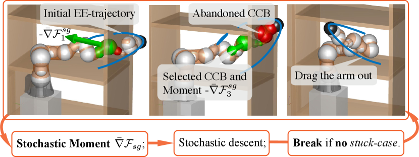
Some studies of deep learning [34, 24, 23, 35] propose stochastic gradient descent (SGD) for learning objects with noisy or sparse gradients. They optimize the objective function consisting of sub-functions in low coupling. Because of the higher robustness of Adam [23] during the function variation, we adopt its moment adaptation method and propose STOMA (Algorithm 3, Figure 2(b)) in the stuck case. This section will first illustrate how to generate a stochastic gradient (SG), detect the stuck case, and introduce how to accelerate SGD with momentum adaptation.
IV-C1 SG generation and Stuck case check
Since (6) reveals that the whole objective functional uses the penalty factor to gather the GP prior and obstacle information which accumulates the sub-functions calculated by collision-check balls (CCBs) in discrete time, we generate an SG
| (15) |
in the Functional, Time, and Space scales:
(i) Functional: We select the penalty factor .
(ii) Time: We select a set whose element is the number of intervals of two support waypoints to gain a sub-gradient for collision-check:
| (16) |
where (5) generates the upsampling matrix with the set to map the randomly upsampled gradient
into the gradient of with .
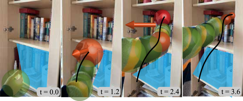
(iii) Space: The intuition of the Space rule comes from the collision avoidance of a human arm on a bookshelf in Figure 2(a). When a participant stretches for an object, he makes sequential reflexes, stimulated by the exterior forces (orange arrow) affecting the danger parts (orange/red balls), in response to the body-obstacle collision. It indicates that the collision risk rises from shoulder to hand because the number of orange/red balls rises from shoulder to hand. So we first reconstruct each rigid body of a tandem manipulator by the geometrically connected CCBs. Next, we build each sub-problem (i.e., the collision avoidance of a single CCB) from shoulder to end-effector, considering the risk variation. Then is calculated by accumulating the CCB-gradients from nearby shoulder up to nearby end-effector:
| (17) |
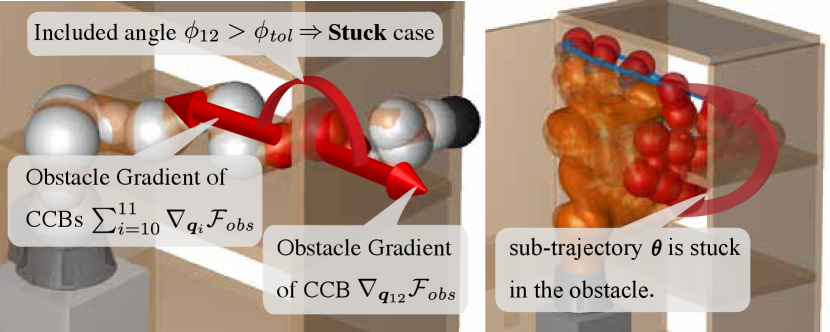
where contains the joints actuating CCB-, and is the included angle between ’s gradient and the accumulated gradient (from to ). The random tolerance angle generates SG in the Space scale by the random rejection of with , meaning that the space stochasticity will vanish when .
(iv) Stuck case: Though, unlike the robot-arm, dragged out by the SG (Figure 2(b)), the stuck case cannot occur during the human-arm avoidance (Figure 2(a)), we can still imagine how confused a human-arm reflex is when a pair of opposite forces stimulate it. So we select a constant to detect the stuck case confusing the collision-free planning. Figure 3 visualizes how an arm is stuck in an obstacle when and how a sub-trajectory containing a series of arms is stuck. We do not adopt the pair-wise check because the risk variates among different parts, and it is more efficient for the stuck check by a constant to synchronize with the SG generation by a random .
IV-C2 Update rules
Adam [23] adopts the piecewise production of gradients and uses EMA from the initial step up to the current step and the bias correction method for the adaptive momentum estimation. Our work uses the squared -norm of SG to estimate and adopt EMA and bias correction for 2nd-momenta estimation:
| (18) |
As shown in Algorithm 3, we adopt the AGD rules [19] rather than the EMA with bias correction for first-momentum adaption. ’s update rules are also reset as
| (19) |
In this way, the descent process, approximately bounded by a -sized trust region, accelerates via the -linear interpolation between the conservative step and the accelerated step driven by and correspondingly. Then the process varies from the lag state guided by to the shifting one guided by with value. Since the SGD is roughly Lipschitz continuous, we get
where and simplify and , and
according to lines 3, 3, 3 of Algorithm 3. Combining the Cauchy-Schwarz inequation, we get
Then through the accumulation from to , we get
where and with .
In sight of the stochasticity of and its gradient and presuming , we get
| (20) |
where is the fraction of and trust region box , and .
Figure 2(b) illustrates how a robot reflexes to the stuck case like the human in Figure 2(a), following the update rules in SgdIter. To improve the efficiency and reliability, we nest the above SGD (i.e., SgdIter) in reSgdIter. Once the SGD is restarted, we select the trajectory with the lowest cost from the sample set to reinitialize the next SGD, whose maximum number is selected randomly in .
V EXPERIMENT
This section will first introduce the objective functional implementation in Section V-A. Then it will detail the benchmark and parameter setting in Sections V-B1 & V-B2 and analyze the benchmark results in Section V-B3.
V-A Implementation details
V-A1 GP prior
We assume the velocity is constant and gain the GMM and GP-prior (1) to reduce the dimension. Our benchmark uses support states with intervals (116 states in total) for iSAGO and GPMP2, 116 states for STOMP and CHOMP, 12 and 58 states for TrajOpt444Since TrajOpt proposes a swept-out area between support waypoints for continuous-time safety, we choose TrajOpt-12 for safety validation and TrajOpt-58 to ensure the dimensional consistency of the benchmark. , and MaxConnectionDistance for RRT-Connect. All implementations except RRT-Connect apply linear interpolation rather than manual selection to initialize trajectory for a fair comparison.
V-A2 Collision cost function
V-A3 Motion constraints
The motion cost function in GPMP [2] is adopted to drive the robot under the preplanned optimal collision-free trajectory in the real world.
V-B Evaluation
V-B1 Setup for benchmark
This paper benchmarks iSAGO against the numerical planners (CHOMP [1], TrajOpt [3], GPMP2 [2]) and the sampling planners (STOMP [8], RRT-Connect [7]) on a 7-DoF robot (LBR-iiwa) and a 6-DoF robot (AUBO-i5). Since the benchmark executes in MATLAB, we use BatchTrajOptimize3DArm of GPMP2-toolbox to implement GPMP2, plannarBiRRT with 20s maximum time for RRT-Connect, fmincon555We use optimoptions(’fmincon’,’Algorithm’,’trust-region-reflective’,’SpecifyObjectiveGradient’, true) to apply fmincon for the trust-region method like TrajOpt and calculates ObjectiveGradient analytically and Aeq (a matrix whose rows are the constraint gradients) by numerical differentiation. for TrajOpt, hmcSampler666Our benchmark defines an hmcSampler object whose logarithm probabilistic density function logpdf is defined by (6), uses hmcSampler.drawSamples for HMC adopted by CHOMP. for CHOMP, and mvnrnd777STOMP samples the noise trajectories by mvnrnd and updates the trajectory via projected weighted averaging. for STOMP. Since all of them are highly tuned in their own studies, our benchmark uses their default settings.
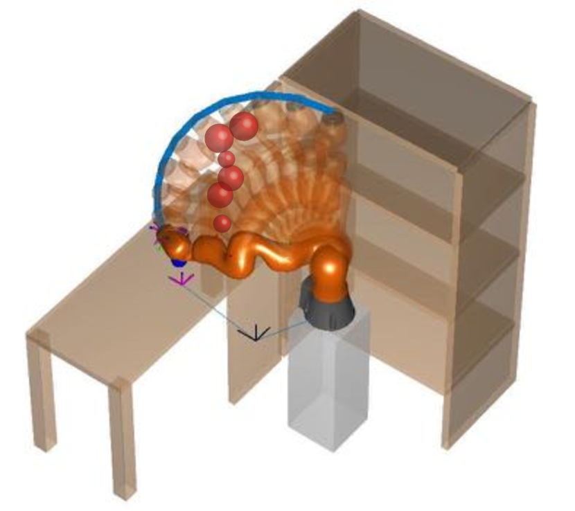
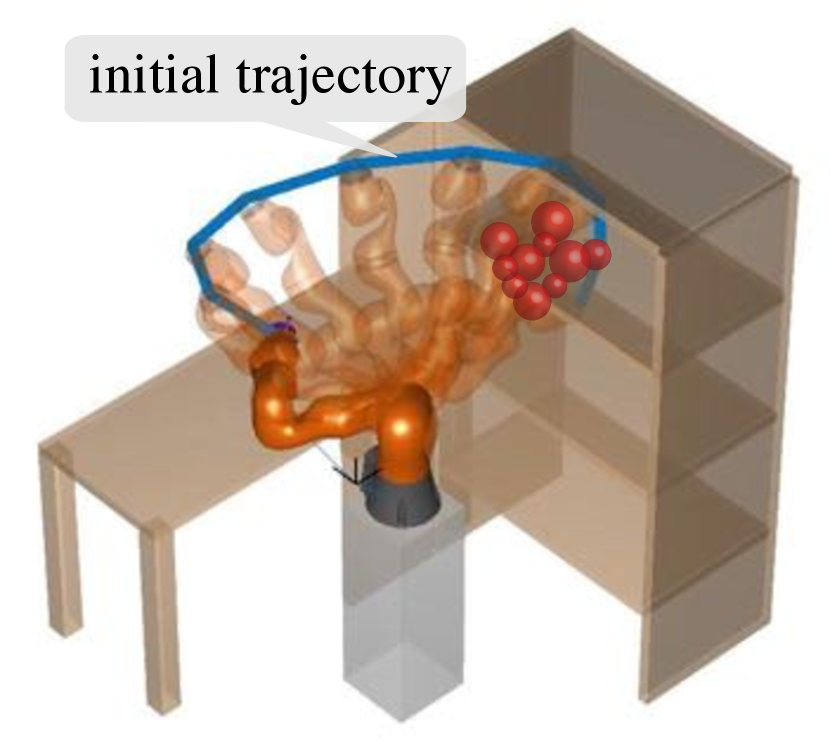
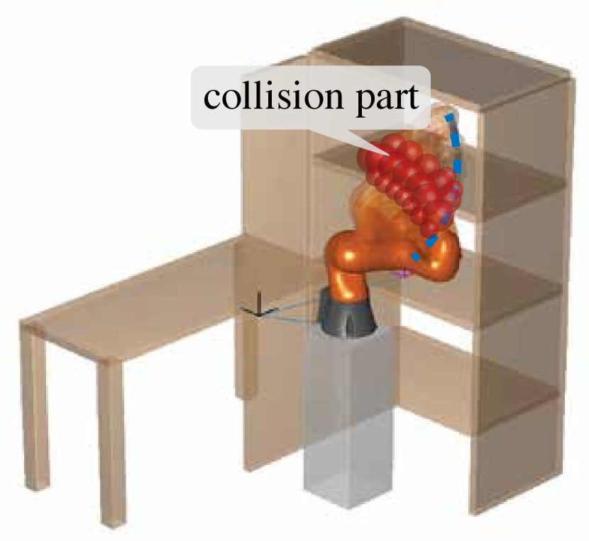
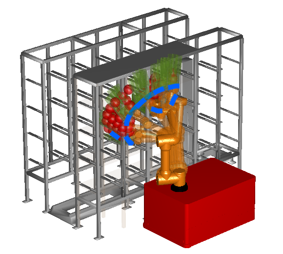
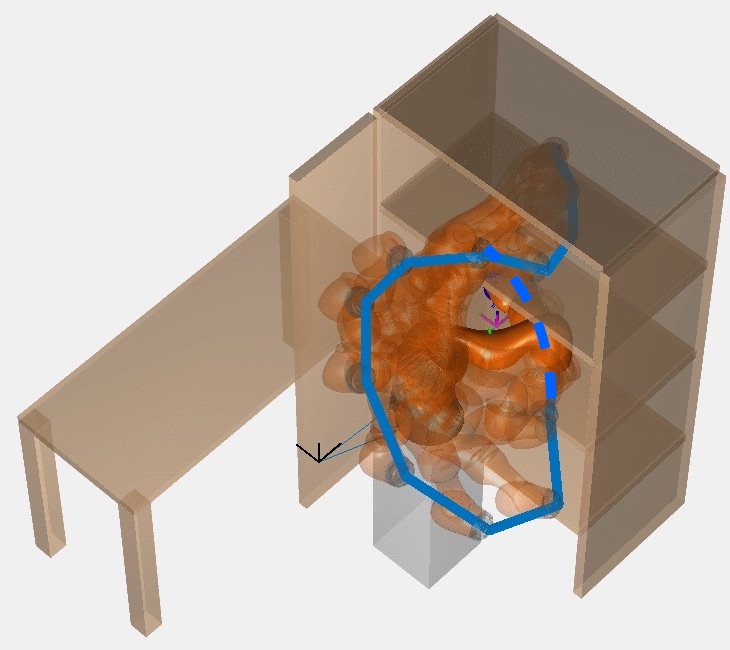
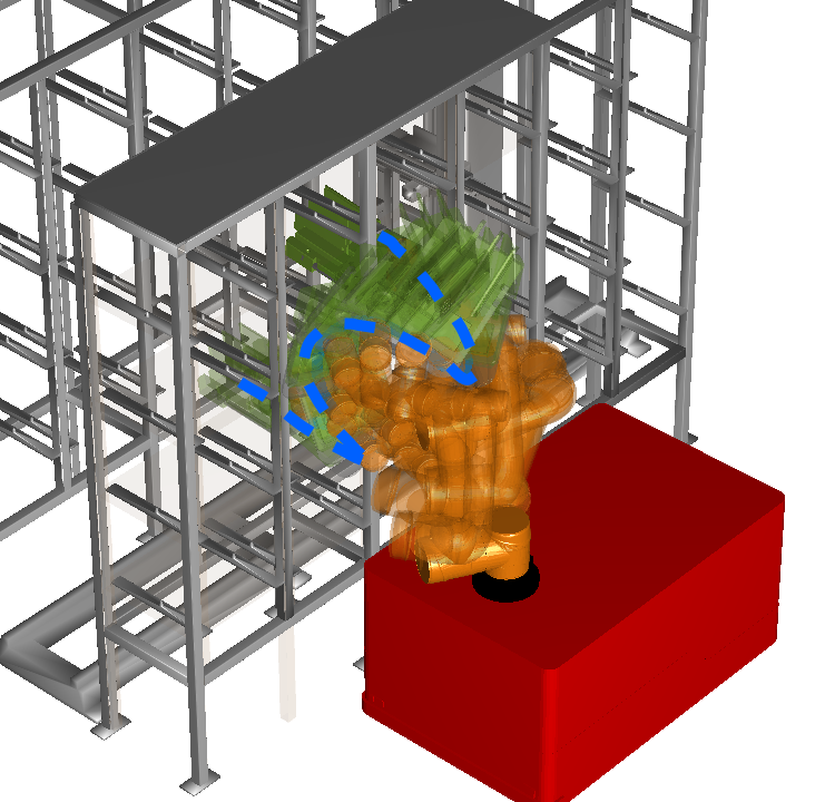
To illustrate the competence of iSAGO for planning tasks, we conduct 25 experiments on LBR-iiwa at a bookshelf and 12 experiments on AUBO-i5 at a storage shelf. We categorize all tasks into 3 classes (A, B, and C) whose planning difficulty rises with the stuck cases in the initial trajectory increase. Figure 4 visually validates our classification because the number of red in-collision CCBs increases from Task A-1 to Task C-3. Considering the difficulty of different classes, we first generate 2 tasks of class A, 3 tasks of class B, and 4 tasks of class C for LBR-iiwa (Figures 4(a)-4(c)). Then we generate 6 tasks of class C for AUBO-i5 (Figures 4(d)). Each task consists of 2 to 4 problems888Since LBR-iiwa has 7 DoFs, meaning infinite solutions for the same goal constraint, our benchmark uses LM [14] with random initial points to generate different goal states. So one planning task of LBR-iiwa with the same goal constraint has several problems with different goal states. Meanwhile, each task of AUBO-i5 has two problems with the same initial state and goal constraint because the same goal constraint has only one solution for the 6-DoF, and we switch yaw-angle in for each. with the same initial state and goal constraint. Moreover, we compare iSAGO with SAGO to show the efficiency of the incremental method and compare SAGO with STOMA or AGD to show the efficiency or reliability of the mixed optimization.
V-B2 Parameter setting
Since STOMA (Algorithm 3, Figure 2(b)) proceeds SGD roughly contained in a -sized trust-region with -damped EMA of historical momenta, this section first tunes these two parameters, then the others.
According to abundant experiences, we tune the key parameters , and conduct 10 different class C tasks for each pair of parameters. Table I indicates that the SGD rate increases with -expansion. In contrast, the success rate decreases with the excessive (i.e., too high or too low). Moreover, the SGD rate increases with -shrink while the success rate decreases with -shrink. All in all, iSAGO performs more stable with a smaller step-size , hampering local minima’s overcoming. Meanwhile, it combines less historical momenta to perform faster, reducing the reliability. So we set and .
|
|
0.80 | 0.40 | 0.08 | 0.04 |
|---|---|---|---|---|
| 0.50 | 80 | 1.253 | 90 | 1.898 | 60 | 4.198 | 40 | 6.309 |
| 0.90 | 90 | 2.512 | 100 | 2.463 | 80 | 4.973 | 60 | 8.219 |
| 0.99 | 90 | 2.672 | 100 | 3.089 | 80 | 7.131 | 60 | 12.57 |
-
1
(%) and (s) denote the success rate and average computation time.
Besides and , we set the initial penalty , penalty factor , and filter factor in Algorithm 1. In Algorithm 2, we set the tolerances , , and scaling factor . In Algorithm 3, we set the number of samples , tolerance , and the number of SgdIter . Moreover, we select to check stuck case while to generate SG.
V-B3 Result analysis
| Problem | Our incremental mixed optimization | numerical optimization | probabilistic sampling | ||||||||
| AGD | STOMA | SAGO | iSAGO | TrajOpt-12 | TrajOpt-58 | GPMP2-12 | CHOMP | STOMP | RRT-Connect | ||
| Scr(%) | iiwa_AB | 75 | 97.5 | 100 | 100 | 27.5 | 77.5 | 81.25 | 87.5 | 82.5 | 100 |
| iiwa_C | 8.75 | 87.5 | 91.25 | 93.75 | 3.75 | 8.75 | 11.25 | 30 | 25 | 72.5 | |
| aubo_C | 5 | 71.67 | 83.33 | 88.33 | 3.33 | 6.67 | 11.67 | 26.67 | 25 | 73.33 | |
| Avt(s) | iiwa_AB | 0.278 | 3.031 | 1.714 | 1.145 | 0.127 | 0.495 | 1.294 | 2.728 | 3.080 | 8.92 |
| iiwa_C | 0.288 | 7.622 | 4.284 | 2.132 | 0.232 | 1.108 | 2.464 | 6.989 | 7.691 | 13.65 | |
| aubo_C | 0.343 | 8.584 | 4.812 | 2.413 | 0.245 | 1.119 | 2.610 | 7.588 | 8.640 | 16.02 | |
| Sdt(s) | iiwa_AB | 0.032 | 0.823 | 0.362 | 0.287 | 0.034 | 0.076 | 0.845 | 0.988 | 2.540 | 3.613 |
| iiwa_C | 0.045 | 1.735 | 1.048 | 0.319 | 0.055 | 0.101 | 1.312 | 1.290 | 5.233 | 4.562 | |
| aubo_C | 0.078 | 1.821 | 1.101 | 0.334 | 0.057 | 0.106 | 1.377 | 1.354 | 5.494 | 3.974 | |
-
1
Scr(%), Avt(s) and Sdt(s) denote the success rate, average computation time and standard deviation of computation time, respectively.
-
2
iiwa_AB, iiwa_C and aubo_C denote 16 class A&B problems on LBR-iiwa, 16 class C problems on LBR-iiwa, and 12 class C problems on AUBO-i5, respectively.
Figure 5(a) shows how iSAGO drags a series of in-stuck arms of Figure 4(c) out of the bookshelf by STOMA to grasp a cup located in the middle layer of the bookshelf safely. Meanwhile, Figure 5(b) shows how AUBO-i5 avoids the collision of Figure 4(d) to transfer the green piece between different cells of the storage shelf safely.
Table II shows iSAGO gains the highest success rate compared to the others. The random SgdIter number and AGD help iSAGO gain the fourth solving rate after TrajOpt-12, TrajOpt-58, and GPMP2-12. Though TrajOpt-58 compensates for the continuous safety information leakage of TrajOpt-12 in iiwa_AB, it still cannot escape from the local minima contained by the trust region and gains the second lowest success rate just above TrajOpt-12 in iiwa_C/aubo_C. In contrast, iSAGO successfully descends into an optimum with adaptive stochastic momenta and an appropriate initial trust-region. Thanks to HMC, randomly gaining the Hamiltonian momenta, CHOMP approaches the optimum with the third-highest success rate, whose failures are informed by the deterministic rather than the stochastic gradients. RRT-Connect with a limited time has the highest and the second-highest success rate in iiwa_AB and iiwa_C/aubo_C, respectively. However, a higher rate needs a smaller connection distance which restricts the RRT growth and computation efficiency. Though STOMP is free of gradient calculation, the significant time it takes to resample does a minor effect on feasible searching, mainly limited by the Gauss kernel. As for GPMP2-12 and TrajOpt-58, the LM and trust-region methods help approach the stationary point rapidly. In contrast, the point of iiwa_C/aubo_C has significantly lower feasibility than that in iiwa_A because the initial trajectory of iiwa_C/aubo_C gets stuck deeper.
The comparison between STOMA and SAGO in Table II shows how AGD performs a 45% accelerated descent towards an optimum. The comparison between iSAGO and SAGO indicates a 55% higher efficiency of incremental planning. The 90% lower success rate of AGD than SAGO shows the limitation of the numerical method. It validates that STOMA can modify the manifold with less local minima by randomly selecting sub-functional.
The comparison between iiwa_C and aubo_C in Tables II shows that iSAGO performs better when the feasible solution is nearby the motion constraints. That is because the motion constraint somewhat stabilizes the -sized SGD of STOMA. So the large -sized steps bring a severe disturbance and weaken STOMA’s performance by 20% when obstacles wrap the feasible solution. Meanwhile, the comparison between iiwa_AB and iiwa_C shows that the stuck case reduces the success rate of the numerical method by 90% and validates iSAGO’s higher reliability in a narrow workspace under the same non-manual initial condition.
VI CONCLUSIONS
iSAGO utilizes the mixed information of accelerated (AGD) and stochastic (STOMA) momentum to overcome the body-obstacle stuck cases in a narrow workspace.
(i) STOMA performs an adaptive stochastic descent to avoid the local minima confronted by the numerical methods, and the results show the highest success rate among them.
(ii) AGD integrated by iSAGO accelerates the descent informed by the first-order momenta. The results show it saves the sampling method’s computation resources and gain the fourth solving rate.
(iii) The incremental planning optimizes the sub-planning to elevate the whole-planning rate further. The results show the 55% higher efficiency of iSAGO than SAGO.
References
- [1] M. Zucker, N. Ratliff, A. D. Dragan, M. Pivtoraiko, M. Klingensmith, C. M. Dellin, J. A. Bagnell, and S. S. Srinivasa, “Chomp: Covariant hamiltonian optimization for motion planning,” The International Journal of Robotics Research, vol. 32, no. 9-10, pp. 1164–1193, 2013.
- [2] M. Mukadam, J. Dong, X. Yan, F. Dellaert, and B. Boots, “Continuous-time gaussian process motion planning via probabilistic inference,” The International Journal of Robotics Research, vol. 37, no. 11, pp. 1319–1340, 2018.
- [3] J. Schulman, J. Ho, A. X. Lee, I. Awwal, H. Bradlow, and P. Abbeel, “Finding locally optimal, collision-free trajectories with sequential convex optimization.” in Robotics: science and systems, vol. 9, no. 1. Citeseer, 2013, pp. 1–10.
- [4] M. Bhardwaj, B. Boots, and M. Mukadam, “Differentiable gaussian process motion planning,” in 2020 IEEE International Conference on Robotics and Automation (ICRA), May 2020, pp. 10 598–10 604.
- [5] L. E. Kavraki, M. N. Kolountzakis, and J. . Latombe, “Analysis of probabilistic roadmaps for path planning,” IEEE Transactions on Robotics and Automation, vol. 14, no. 1, pp. 166–171, Feb 1998.
- [6] S. M. LaValle et al., “Rapidly-exploring random trees: A new tool for path planning,” 1998.
- [7] J. J. Kuffner and S. M. LaValle, “Rrt-connect: An efficient approach to single-query path planning,” in Proceedings 2000 ICRA. Millennium Conference. IEEE International Conference on Robotics and Automation. Symposia Proceedings (Cat. No.00CH37065), vol. 2, April 2000, pp. 995–1001 vol.2.
- [8] M. Kalakrishnan, S. Chitta, E. Theodorou, P. Pastor, and S. Schaal, “Stomp: Stochastic trajectory optimization for motion planning,” in 2011 IEEE International Conference on Robotics and Automation, May 2011, pp. 4569–4574.
- [9] S. Karaman and E. Frazzoli, “Sampling-based algorithms for optimal motion planning,” The international journal of robotics research, vol. 30, no. 7, pp. 846–894, 2011.
- [10] P. Rajendran, S. Thakar, A. M. Kabir, B. C. Shah, and S. K. Gupta, “Context-dependent search for generating paths for redundant manipulators in cluttered environments,” in 2019 IEEE/RSJ International Conference on Intelligent Robots and Systems (IROS), 2019, pp. 5573–5579.
- [11] C. Park, J. Pan, and D. Manocha, “Itomp: Incremental trajectory optimization for real-time replanning in dynamic environments,” in Proceedings of the Twenty-Second International Conference on International Conference on Automated Planning and Scheduling, ser. ICAPS’12. AAAI Press, 2012, pp. 207–215.
- [12] K. Shirley, “Inference from simulations and monitoring convergence,” Handbook of Markov Chain Monte Carlo, May 2011.
- [13] M. Kaess, H. Johannsson, R. Roberts, V. Ila, J. J. Leonard, and F. Dellaert, “isam2: Incremental smoothing and mapping using the bayes tree,” The International Journal of Robotics Research, vol. 31, no. 2, pp. 216–235, 2012.
- [14] K. Levenberg, “A method for the solution of certain non-linear problems in least squares,” Quarterly of Applied Mathematics, vol. 2, no. 2, pp. 164–168, 1944.
- [15] R. H. Byrd, J. C. Gilbert, and J. Nocedal, “A trust region method based on interior point techniques for nonlinear programming,” Mathematical programming, vol. 89, no. 1, pp. 149–185, 2000.
- [16] J. Ichnowski, Y. Avigal, V. Satish, and K. Goldberg, “Deep learning can accelerate grasp-optimized motion planning,” Science Robotics, vol. 5, no. 48, p. eabd7710, 2020.
- [17] A. Kuntz, C. Bowen, and R. Alterovitz, “Fast anytime motion planning in point clouds by interleaving sampling and interior point optimization,” in Robotics Research, N. M. Amato, G. Hager, S. Thomas, and M. Torres-Torriti, Eds. Cham: Springer International Publishing, 2020, pp. 929–945.
- [18] Y. Nesterov, “A method for unconstrained convex minimization problem with the rate of convergence o (1/k^ 2),” in Doklady an ussr, vol. 269, 1983, pp. 543–547.
- [19] S. Ghadimi and G. Lan, “Accelerated gradient methods for nonconvex nonlinear and stochastic programming,” Mathematical Programming, vol. 156, no. 1-2, pp. 59–99, 2016.
- [20] W. Su, S. Boyd, and E. Candes, “A differential equation for modeling nesterov’s accelerated gradient method: Theory and insights,” in Advances in Neural Information Processing Systems 27, Z. Ghahramani, M. Welling, C. Cortes, N. D. Lawrence, and K. Q. Weinberger, Eds. Curran Associates, Inc., 2014, pp. 2510–2518.
- [21] A. C. Wilson, B. Recht, and M. I. Jordan, “A lyapunov analysis of momentum methods in optimization,” 2018.
- [22] L. Bottou, “Large-scale machine learning with stochastic gradient descent,” in Proceedings of COMPSTAT’2010, Y. Lechevallier and G. Saporta, Eds. Heidelberg: Physica-Verlag HD, 2010, pp. 177–186.
- [23] D. P. Kingma and J. Ba, “Adam: A method for stochastic optimization,” arXiv preprint arXiv:1412.6980, 2014.
- [24] H. Geoffrey, N. Srivastava, and K. Swersky, “Neural networks for machine learning lecture 6a overview of mini-batch gradient descent,” Department of Computer Science, University of Toronto, Tech. Rep. 14, 02 2012.
- [25] X. Wu and M. W. Mueller, “In-flight range optimization of multicopters using multivariable extremum seeking with adaptive step size,” in 2020 IEEE/RSJ International Conference on Intelligent Robots and Systems (IROS), 2020, pp. 1545–1550.
- [26] K. Solovey, O. Salzman, and D. Halperin, “New perspective on sampling-based motion planning via random geometric graphs,” The International Journal of Robotics Research, vol. 37, no. 10, pp. 1117–1133, 2018.
- [27] E. W. Dijkstra, “A note on two problems in connexion with graphs,” Numerische Mathematik, vol. 1, no. 1, pp. 269–271, 1959.
- [28] A. G. Hofmann, E. Fernandez, J. Helbert, S. D. Smith, and B. C. Williams, “Reactive integrated motion planning and execution,” in Twenty-Fourth International Joint Conference on Artificial Intelligence, 2015.
- [29] L. Petrović, J. Peršić, M. Seder, and I. Marković, “Stochastic optimization for trajectory planning with heteroscedastic gaussian processes,” in 2019 European Conference on Mobile Robots (ECMR), 2019, pp. 1–6.
- [30] T. Osa, “Multimodal trajectory optimization for motion planning,” The International Journal of Robotics Research, vol. 39, no. 8, pp. 983–1001, 2020.
- [31] J. Nocedal and S. Wright, Numerical optimization. Springer Science & Business Media, 2006.
- [32] Y. Nesterov, Introductory lectures on convex optimization: A basic course. Springer Science & Business Media, 2013, vol. 87.
- [33] B. O’Donoghue and E. Candès, “Adaptive restart for accelerated gradient schemes,” Foundations of Computational Mathematics, vol. 15, no. 3, pp. 715–732, 2015.
- [34] J. Duchi, E. Hazan, and Y. Singer, “Adaptive subgradient methods for online learning and stochastic optimization,” J. Mach. Learn. Res., vol. 12, pp. 2121–2159, July 2011.
- [35] I. Goodfellow, Y. Bengio, and A. Courville, Deep learning. MIT press, 2016.