footnotesection

Index theorems for
uniformly elliptic operators

Alexander Engel

Abstract

We generalize Roe’s index theorem for graded generalized Dirac operators on amenable manifolds to multigraded elliptic uniform pseudodifferential operators.

The generalization will follow from a local index theorem that is valid on any manifold of bounded geometry. This local formula incorporates the uniform estimates present in the definition of uniform pseudodifferential operators.

Fakultät für Mathematik
Universität Regensburg
93040 Regensburg, GERMANY
alexander.engel@mathematik.uni-regensburg.de

1 Introduction

Recall the following index theorem of Roe for amenable manifolds (with notation adapted to the one used in this article):

Theorem ([Roe88a, Theorem 8.2]).

Let $M$ be a Riemannian manifold of bounded geometry and $D$ a generalized Dirac operator associated to a graded Dirac bundle $S$ of bounded geometry over $M$ .

Let $(M_{i})_{i}$ be a Følner sequence¹¹1That is to say, for every $r>0$ we have $\frac{\operatorname{vol}B_{r}(\partial M_{i})}{\operatorname{vol}M_{i}}\stackrel{{\scriptstyle i\to\infty}}{{\longrightarrow}}0$ . Manifolds admitting such a sequence are called amenable. for $M$ , $\tau\in(\ell^{\infty})^{\ast}$ a linear functional associated to a free ultrafilter on $\mathbb{N}$ , and $\theta$ the corresponding trace on the uniform Roe algebra of $M$ .

Then we have

\theta(\mu_{u}(D))=\tau\Big{(}\frac{1}{\operatorname{vol}M_{i}}\int_{M_{i}}\operatorname{ind}(D)\Big{)}.

Here $\operatorname{ind}(D)$ is the usual integrand for the topological index of $D$ in the Atiyah–Singer index formula, so the right hand side is topological in nature. On the left hand side of the formula we have the coarse index class $\mu_{u}(D)\in K_{0}(C_{u}^{\ast}(M))$ of $D$ in the $K$ -theory of the uniform Roe algebra of $M$ evaluated under the trace $\theta$ . This is an analytic expression and may be computed as $\theta(\mu_{u}(D))=\tau\Big{(}\frac{1}{\operatorname{vol}M_{i}}\int_{M_{i}}\operatorname{tr}_{s}k_{f(D)}(x,x)\ dx\Big{)}$ , where $k_{f(D)}(x,y)$ is the integral kernel of the smoothing operator $f(D)$ , where $f$ is an even Schwartz function with $f(0)=1$ .

In this article we will generalize this theorem to all multigraded, elliptic, symmetric uniform pseudodifferential operators. So especially we also encompass Toeplitz operators since they are included in the ungraded case. This generalization will follow from a local index theorem that will hold on any manifold of bounded geometry, i.e., without an amenability assumption on $M$ .

Let us state our local index theorem in the formulation using twisted Dirac operators associated to spin^c structures:

Theorem A (Theorem 1).

Let $M$ be an $m$ -dimensional spin^c manifold of bounded geometry and without boundary. Denote the associated Dirac operator by $D$ .

Then we have the following commutative diagram:

where in the top row $\ast$ is either $0$ or $1$ and in the bottom row $\ast$ is either $\mathrm{ev}$ or $\mathrm{odd}$ .

Here $K_{m-\ast}^{u}(M)$ is uniform $K$ -homology of $M$ invented by Špakula [Špa09] and $K_{u}^{\ast}(M)$ is the corresponding uniform $K$ -theory which we will recall in Section 2.3. The map $-\cap[D]$ is the cap product and that it is an isomorphism was shown in [Eng15a, Section 4.4]. Moreover, $H_{b,\mathrm{dR}}^{\ast}(M)$ denotes the bounded de Rham cohomology of $M$ and $\operatorname{ind}(D)$ the topological index class of $D$ in there. Furthermore, $H^{u,\mathrm{dR}}_{m-\ast}(M)$ is the uniform de Rham homology of $M$ to be defined in Section 3.2 via Connes’ cyclic cohomology, and that it is Poincaré dual to bounded de Rham cohomology is proved in Theorem 10. Finally, let us note that we will also prove in Section 3.3 that the Chern characters induce isomorphisms after a certain completion that also kills torsion, similar to the case of compact manifolds.

Using a series of steps as in Connes’ and Moscovici’s proof of [CM90, Theorem 3.9] we will generalize the above computation of the Poincaré dual of $(\alpha_{\ast}\circ\operatorname{ch}^{\ast})([D])\in H^{u,\mathrm{dR}}_{m-\ast}(M)$ to symmetric and elliptic uniform pseudodifferential operators:

Theorem B (Theorem 3 and Remark 5).

Let $M$ be an oriented Riemannian manifold of bounded geometry and without boundary, and $P$ be a symmetric and elliptic uniform pseudodifferential operator of positive order.

Then $\operatorname{ind}(P)\in H_{b,\mathrm{dR}}^{\ast}(M)$ is the Poincaré dual of $(\alpha_{\ast}\circ\operatorname{ch}^{\ast})([P])\in H^{u,\mathrm{dR}}_{\ast}(M)$ .

Using the above local index theorem we will derive as a corollary the following local index formula:

Corollary C (Corollary 7).

Let $[\varphi]\in H_{c,\mathrm{dR}}^{k}(M)$ be a compactly supported cohomology class and define the analytic index $\operatorname{ind}_{[\varphi]}(P)$ as Connes–Moscovici [CM90] for $P$ being a multigraded, symmetric, elliptic uniform pseudodifferential operator of positive order. Then we have

\operatorname{ind}_{[\varphi]}(P)=\int_{M}\operatorname{ind}(P)\wedge[\varphi]

and this pairing is continuous, i.e., $\int_{M}\operatorname{ind}(P)\wedge[\varphi]\leq\|\operatorname{ind}(P)\|_{\infty}\cdot\|[\varphi]\|_{1}$ , where $\|-\|_{\infty}$ denotes the sup-seminorm on $H_{b,\mathrm{dR}}^{m-k}(M)$ and $\|-\|_{1}$ the $L^{1}$ -seminorm on $H_{c,\mathrm{dR}}^{k}(M)$ .

Note that the corollary reads basically the same as the local index formula of Connes and Moscovici [CM90]. The fundamentally new thing in it is the continuity statement for which we need the uniformity assumption for $P$ .

As a second corollary to the above local index theorem we will, as already written, derive the generalization of Roe’s index theorem for amenable manifolds.

Corollary D (Corollary 20).

Let $M$ be a manifold of bounded geometry and without boundary, let $(M_{i})_{i}$ be a Følner sequence for $M$ and let $\tau\in(\ell^{\infty})^{\ast}$ be a linear functional associated to a free ultrafilter on $\mathbb{N}$ . Denote the from the choice of Følner sequence and functional $\tau$ resulting functional on $K_{0}(C_{u}^{\ast}(M))$ by $\theta$ .

Then for both $p\in\{0,1\}$ , every class $[P]\in K_{p}^{u}(M)$ with $P$ being a $p$ -graded, symmetric, elliptic uniform pseudodifferential operator over $M$ , and every $u\in K_{u}^{p}(M)$ we have

\langle u,[P]\rangle_{\theta}=\langle\operatorname{ch}(u)\wedge\operatorname{ind}(P),[M]\rangle_{(M_{i})_{i},\tau}.

Roe’s theorem [Roe88a] is the special case where $P=D$ is a graded (i.e., $p=0$ ) Dirac operator and $u=[\mathbb{C}]$ is the class in $K_{u}^{0}(M)$ of the trivial, $1$ -dimensional vector bundle over $M$ .

To put the above index theorems into context, let us consider manifolds with cylindrical ends. These are the kind of non-compact manifolds which are studied to prove for example the Atiyah–Patodi–Singer index theorem. In the setting of this paper, the relevant algebra would be that of bounded functions with bounded derivatives, whereas in papers like [Mel95] or [MN08] one imposes conditions at infinity like rapid decay of the integral kernels (see the definition of the suspended algebra in [Mel95, Section 1]).

Note that this global index theorem arising from a Følner sequence is just a special case of a certain rough index theory, where one pairs classes from the so-called rough cohomology with classes in the $K$ -theory of the uniform Roe algebra, and Følner sequences give naturally classes in this rough cohomology. For details see the thesis [Mav95] of Mavra. It seems that it should be possible to combine the above local index theorem with this rough index theory, since it is possible in the special case of Følner sequences. The author investigated this in [Eng15b].

Let us say a few words about the proofs of the above index theorems for elliptic uniform pseudodifferential operators. Roe used in [Roe88a] the heat kernel method to prove his index theorem for amenable manifolds and therefore, since the heat kernel method does only work for Dirac operators, it can not encompass uniform pseudodifferential operators. So what we will basically do in this paper is to set up all the necessary theory in order to be able to reduce the index problem from pseudodifferential operators to Dirac operators.

The main ingredient is a version of Poincaré duality between uniform $K$ -homology and uniform $K$ -theory, which was proved by the author in [Eng15a, Section 4.4]. With this at our disposal we will then be able to reduce the index problem for elliptic uniform pseudodifferential operators to Dirac operators by proving a uniform version of the Thom isomorphism in order to conclude that symbol classes of elliptic uniform pseudodifferential operators may be represented by symbol classes of Dirac operators. So it remains to show the local index theorem for Dirac operators, but since up to this point we will already have set up all the needed machinery, this proof will be basically the same as the proof of the local index theorem of Connes and Moscovici in [CM90].

The last collection of results that we want to highlight in this introduction are all the various (duality) isomorphisms proved in this paper.

Theorem E (Theorems 14, 8 and 10).

Let $M$ be an $m$ -dimensional manifold of bounded geometry and no boundary. Then the Chern characters induce linear, continuous isomorphisms

K^{\ast}_{u}(M)\operatorname{\bar{\otimes}}\mathbb{C}\cong H_{b,\mathrm{dR}}^{\ast}(M)\text{ and }K^{u}_{\ast}(M)\operatorname{\bar{\otimes}}\mathbb{C}\cong H^{u,\mathrm{dR}}_{\ast}(M),

and we also have the isomorphism

H\!P_{\mathrm{cont}}^{*}(W^{\infty,1}(M))\cong H^{u,\mathrm{dR}}_{*}(M).

If $M$ is oriented we further have the isomorphism

H_{b,\mathrm{dR}}^{\ast}(M)\cong H^{u,\mathrm{dR}}_{m-\ast}(M).

If $M$ is spin^c then we have the Poincaré duality isomorphism $K_{u}^{\ast}(M)\cong K^{\ast}_{m-\ast}(M)$ , which is proved in [Eng15a, Theorem 4.29].

Acknowledgements

This article contains mostly Section 5 of the preprint [Eng15a] which is being split up for easier publication. It arose out of the Ph.D. thesis [Eng14] of the author written at the University of Augsburg.

2 Review of needed material

In this section we review the needed material from the literature. We start with the notion of bounded geometry for Riemannian manifolds, define Sobolev spaces and discuss the Sobolev embedding theorem, and at the end of Section 2.1 we prove the technical Lemma 14 about constructing covers with certain properties on manifolds of bounded geometry. In Section 2.2 we discuss the calculus of uniform pseudodifferential operators that we will use in this paper, and in Section 2.3 we recall the basic facts about uniform $K$ -homology and uniform $K$ -theory.

2.1 Manifolds of bounded geometry

We will recall in this section the notion of bounded geometry for manifolds and for vector bundles and discuss basic facts about uniform $C^{r}$ -spaces and Sobolev spaces on them. Almost all material presented here is already known, and we tried to give proper credits wherever possible. As a genuine reference one might also use Eldering [Eld13, Chapter 2].

Definition 1.

We say that a Riemannian manifold $M$ has bounded geometry, if

•

the curvature tensor and all its derivatives are bounded, i.e.,

$\sup_{x\in M}\|\nabla^{k}\operatorname{Rm}(x)\|<\infty$

for all $k\in\mathbb{N}_{0}$ , and
•

the injectivity radius is uniformly positive, i.e.,

$\inf_{x\in M}\operatorname{inj-rad}_{M}(x)>0.$

If $E\to M$ is a vector bundle with a metric and compatible connection, then $E$ has bounded geometry, if the curvature tensor of $E$ and all its derivatives are bounded.

Examples 2.

The most important examples of manifolds of bounded geometry are coverings of closed Riemannian manifolds equipped with the pull-back metric, homogeneous manifolds with an invariant metric, and leafs in a foliation of a compact Riemannian manifold (Greene [Gre78, lemma on page 91 and the paragraph thereafter]).

For vector bundles, the most important examples are of course again pull-back bundles of bundles over closed manifolds equipped with the pull-back metric and connection, and the tangent bundle of a manifold of bounded geometry. ∎

We now state an important characterization in local coordinates of bounded geometry since it allows one to show that certain local definitions are independent of the chosen normal coordinates.

Lemma 3 ([Shu92, Appendix A1.1]).

Let the injectivity radius of $M$ be positive.

Then the curvature tensor of $M$ and all its derivatives are bounded if and only if for any $0<r<\operatorname{inj-rad}_{M}$ all the transition functions between overlapping normal coordinate charts of radius $r$ are uniformly bounded, as are all their derivatives (i.e., the bounds can be chosen to be the same for all transition functions).

Another fact which we will need about manifolds of bounded geometry is the existence of uniform covers by normal coordinate charts and corresponding partitions of unity. A proof may be found in, e.g., [Shu92, Appendix A1.1] (Shubin addresses the first statement about the existence of such covers actually to the paper [Gro81a] of Gromov).

Lemma 4.

Let $M$ be a manifold of bounded geometry.

For every $0<\varepsilon<\tfrac{\operatorname{inj-rad}_{M}}{3}$ exists a cover of $M$ by normal coordinate charts of radius $\varepsilon$ with the properties that the midpoints of the charts form a uniformly discrete set and that the coordinate charts with double radius $2\varepsilon$ form a uniformly locally finite cover of $M$ .

Furthermore, there is a subordinate partition of unity $1=\sum_{i}\varphi_{i}$ with $\operatorname{supp}\varphi_{i}\subset B_{2\varepsilon}(x_{i})$ , such that in normal coordinates the functions $\varphi_{i}$ and all their derivatives are uniformly bounded (i.e., the bounds do not depend on $i$ ).

If the manifold $M$ has bounded geometry, we have analogous equivalent local characterizations of bounded geometry for vector bundles as for manifolds. The equivalence of the first two bullet points in the next lemma is stated in, e.g., [Roe88a, Proposition 2.5]. Concerning the third bullet point, the author could not find any citable reference in the literature (though both Shubin [Shu92] and Eldering [Eld13] use this as the definition).

Lemma 5.

Let $M$ be a manifold of bounded geometry and $E\to M$ a vector bundle. Then the following are equivalent:

•

$E$ has bounded geometry,
•

the Christoffel symbols $\Gamma_{i\alpha}^{\beta}(y)$ of $E$ with respect to synchronous framings (considered as functions on the domain $B$ of normal coordinates at all points) are bounded, as are all their derivatives, and this bounds are independent of $x\in M$ , $y\in\exp_{x}(B)$ and $i,\alpha,\beta$ , and
•

the matrix transition functions between overlapping synchronous framings are uniformly bounded, as are all their derivatives (i.e., the bounds are the same for all transition functions).

We will now give the definition of uniform $C^{\infty}$ -spaces together with a local characterization on manifolds of bounded geometry. The interested reader is refered to, e.g., the papers [Roe88a, Section 2] or [Shu92, Appendix A1.1] of Roe and Shubin for more information regarding these uniform $C^{\infty}$ -spaces.

Definition 6 ( $C^{r}$ -bounded functions).

Let $f\in C^{\infty}(M)$ . We say that $f$ is a $C_{b}^{r}$ -function, or equivalently that it is $C^{r}$ -bounded, if $\|\nabla^{i}f\|_{\infty}<C_{i}$ for all $0\leq i\leq r$ .

If $M$ has bounded geometry, being $C^{r}$ -bounded is equivalent to the statement that in every normal coordinate chart $|\partial^{\alpha}f(y)|<C_{\alpha}$ for every multiindex $\alpha$ with $|\alpha|\leq r$ (where the constants $C_{\alpha}$ are independent of the chart).

The definition of $C^{r}$ -boundedness and its equivalent characterization in normal coordinate charts for manifolds of bounded geometry make also sense for sections of vector bundles of bounded geometry.

Definition 7 (Uniform $C^{\infty}$ -spaces).

Let $E$ be a vector bundle of bounded geometry over $M$ . We will denote the uniform $C^{r}$ -space of all $C^{r}$ -bounded sections of $E$ by $C_{b}^{r}(E)$ .

Furthermore, we define the uniform $C^{\infty}$ -space $C_{b}^{\infty}(E)$

C_{b}^{\infty}(E):=\bigcap_{r}C_{b}^{r}(E)

which is a Fréchet space.

Now we get to Sobolev spaces on manifolds of bounded geometry. Much of the following material is from [Shu92, Appendix A1.1] and [Roe88a, Section 2], where an interested reader can find more thorough discussions of this matters.

Let $s\in C^{\infty}_{c}(E)$ be a compactly supported, smooth section of some vector bundle $E\to M$ with metric and connection $\nabla$ . For $k\in\mathbb{N}_{0}$ and $p\in[1,\infty)$ we define the global $W^{k,p}$ -Sobolev norm of $s$ by

\|s\|_{W^{k,p}}^{p}:=\sum_{i=0}^{k}\int_{M}\|\nabla^{i}s(x)\|^{p}dx.

(2.1)

Definition 8 (Sobolev spaces $W^{k,p}(E)$ ).

Let $E$ be a vector bundle which is equipped with a metric and a connection. The $W^{k,p}$ -Sobolev space of $E$ is the completion of $C^{\infty}_{c}(E)$ in the norm $\|-\|_{W^{k,p}}$ and will be denoted by $W^{k,p}(E)$ .

If $E$ and $M^{m}$ both have bounded geometry than the Sobolev norm (2.1) for $1<p<\infty$ is equivalent to the local one given by

\|s\|_{W^{k,p}}^{p}\stackrel{{\scriptstyle\text{equiv}}}{{=}}\sum_{i=1}^{\infty}\|\varphi_{i}s\|^{p}_{W^{k,p}(B_{2\varepsilon}(x_{i}))},

(2.2)

where the balls $B_{2\varepsilon}(x_{i})$ and the subordinate partition of unity $\varphi_{i}$ are as in Lemma 4, we have chosen synchronous framings and $\|-\|_{W^{k,p}(B_{2\varepsilon}(x_{i}))}$ denotes the usual Sobolev norm on $B_{2\varepsilon}(x_{i})\subset\mathbb{R}^{m}$ . This equivalence enables us to define the Sobolev norms for all $k\in\mathbb{R}$ , see Triebel [Tri10] and Große–Schneider [GS13]. There are some issues in the case $p=1$ , see the discussion by Triebel [Tri83, Section 2.2.3], [Tri10, Remark 4 on Page 13].

Assuming bounded geometry, the usual embedding theorems are true:

Theorem 9 ([Aub98, Theorem 2.21]).

Let $E$ be a vector bundle of bounded geometry over a manifold $M^{m}$ of bounded geometry and without boundary.

Then we have for all values $(k-r)/m>1/p$ continuous embeddings

W^{k,p}(E)\subset C^{r}_{b}(E).

We define the space

W^{\infty,p}(E):=\bigcap_{k\in\mathbb{N}_{0}}W^{k,p}(E)

(2.3)

and equip it with the obvious Fréchet topology. The Sobolev Embedding Theorem tells us now that we have for all $p$ a continuous embedding

W^{\infty,p}(E)\hookrightarrow C^{\infty}_{b}(E).

Finally, we come to a technical statement (Lemma 14) about the existence of open covers with special properties on manifolds of bounded geometry, similar to Lemma 4. As a preparation we first have to recall some facts about simplicial complexes of bounded geometry and corresponding triangulations of manifolds of bounded geometry.

Definition 10 (Bounded geometry simplicial complexes).

A simplicial complex has bounded geometry if there is a uniform bound on the number of simplices in the link of each vertex.

A subdivision of a simplicial complex of bounded geometry with the properties that

•

each simplex is subdivided a uniformly bounded number of times on its $n$ -skeleton, where the $n$ -skeleton is the union of the $n$ -dimensional sub-simplices of the simplex, and that
•

the distortion $\operatorname{length}(e)+\operatorname{length}(e)^{-1}$ of each edge $e$ of the subdivided complex is uniformly bounded in the metric given by barycentric coordinates of the original complex,

is called a uniform subdivision.

Theorem 11 (Attie [Att94, Theorem 1.14]).

Let $M$ be a manifold of bounded geometry and without boundary.

Then $M$ has a triangulation as a simplicial complex of bounded geometry such that the metric given by barycentric coordinates is bi-Lipschitz equivalent²²2Two metric spaces $X$ and $Y$ are said to be bi-Lipschitz equivalent if there is a homeomorphism $f\colon X\to Y$ with $\tfrac{1}{C}d_{X}(x,x^{\prime})\leq d_{Y}(f(x),f(x^{\prime}))\leq Cd_{X}(x,x^{\prime})$ for all $x,x^{\prime}\in X$ and some constant $C>0$ . to the one on $M$ induced by the Riemannian structure. This triangulation is unique up to uniform subdivision.

Conversely, if $M$ is a simplicial complex of bounded geometry which is a triangulation of a smooth manifold, then this smooth manifold admits a metric of bounded geometry with respect to which it is bi-Lipschitz equivalent to $M$ .

Remark 12.

Attie uses in [Att94] a weaker notion of bounded geometry as we do: additionally to a uniformly positive injectivity radius he only requires the sectional curvatures to be bounded in absolute value (i.e., the curvature tensor is bounded in norm), but he assumes nothing about the derivatives (see [Att94, Definition 1.4]). But going into his proof of [Att94, Theorem 1.14], we see that the Riemannian metric constructed for the second statement of the theorem is actually of bounded geometry in our strong sense (i.e., also with bounds on the derivatives of the curvature tensor).

As a corollary we get that for any manifold of bounded geometry in Attie’s weak sense there is another Riemannian metric of bounded geometry in our strong sense that is bi-Lipschitz equivalent the original one (in fact, this bi-Lipschitz equivalence is just the identity map of the manifold, as can be seen from the proof).

The last auxiliary lemma (before we come to the crucial Lemma 14) is about coloring covers of manifolds with only finitely many colors:

Lemma 13.

Let a covering $\{U_{\alpha}\}$ of $M$ with finite multiplicity be given. Then there exists a coloring of the subsets $U_{\alpha}$ with finitely many colors such that no two intersecting subsets have the same color.

Proof 2.1.

Construct a graph whose vertices are the subsets $U_{\alpha}$ and two vertices are connected by an edge if the corresponding subsets intersect. We have to find a coloring of this graph with only finitely many colors where connected vertices do have different colors.

To do this, we firstly use the theorem of de Bruijin–Erdös stating that an infinite graph may be colored by $k$ colors if and only if every of its finite subgraphs may be colored by $k$ colors (one can use the Lemma of Zorn to prove this).

Secondly, since the covering has finite multiplicity it follows that the number of edges attached to each vertex in our graph is uniformly bounded from above, i.e., the maximum vertex degree of our graph is finite. But this also holds for every subgraph of our graph, with the maximum vertex degree possibly only decreasing by passing to a subgraph. Now a simple greedy algorithm shows that every finite graph may be colored with one more color than its maximum vertex degree: just start by coloring a vertex with some color, go to the next vertex and use an admissible color for it, and so on.

Lemma 14.

Let $M$ be a manifold of bounded geometry and without boundary.

Then there is an $\varepsilon>0$ and a countable collection of uniformly discretely distributed points $\{x_{i}\}_{i\in I}\subset M$ such that $\{B_{\varepsilon}(x_{i})\}_{i\in I}$ is a uniformly locally finite cover of $M$ . We can additionally arrange such that it has the following two properties:

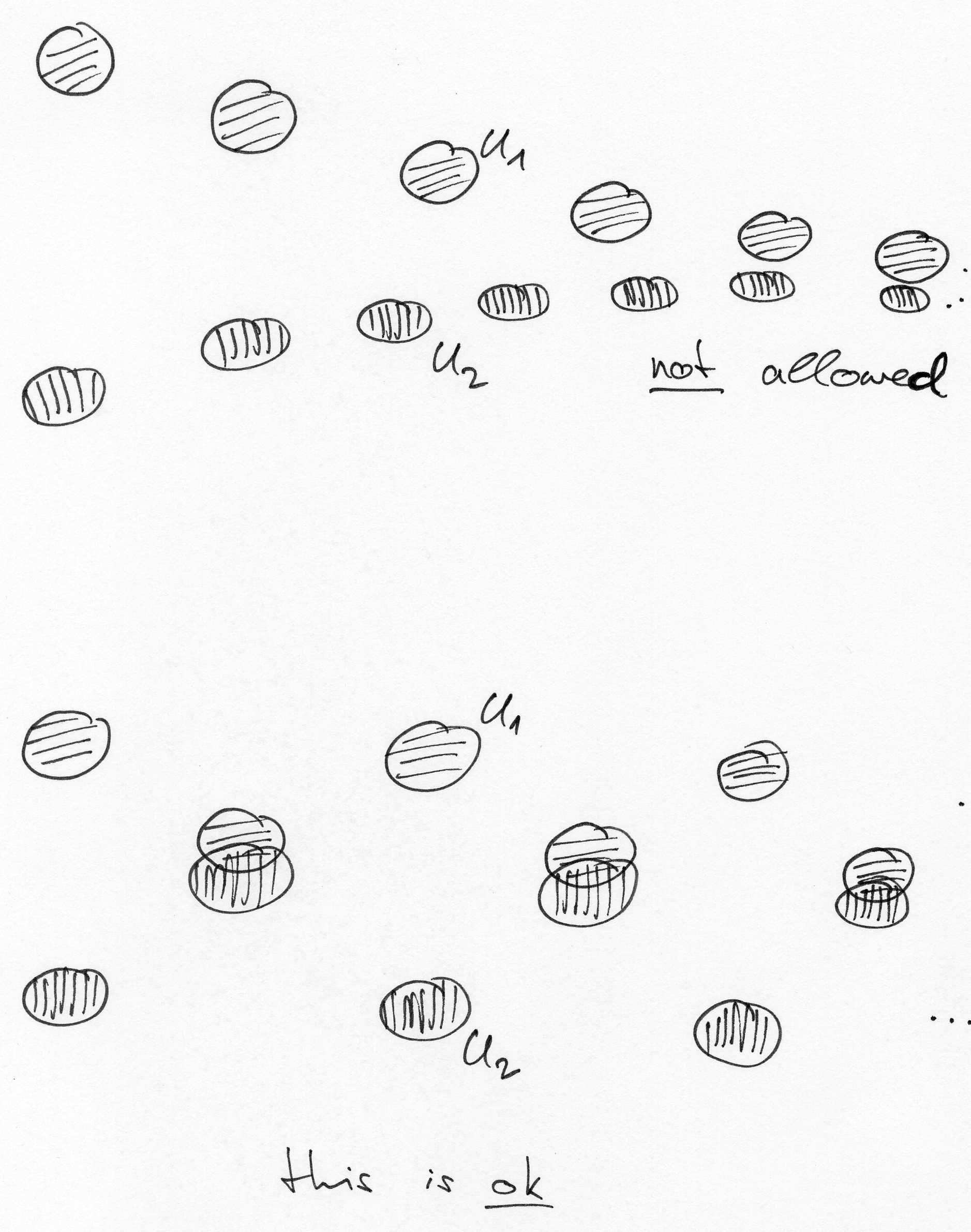
1.

It is possible to partition $I$ into a finite amount of subsets $I_{1},\ldots,I_{N}$ such that for each $1\leq j\leq N$ the subset $U_{j}:=\bigcup_{i\in I_{j}}B_{\varepsilon}(x_{i})$ is a disjoint union of balls that are a uniform distance apart from each other, and such that for each $1\leq K\leq N$ the connected components of $U_{K}:=U_{1}\cup\ldots\cup U_{k}$ are also a uniform distance apart from each other (see Figure 1).
2.

Instead of choosing balls $B_{\varepsilon}(x_{i})$ to get our cover of $M$ it is possible to choose other open subsets such that additionally to the property from Point 1 for any distinct $1\leq m,n\leq N$ the symmetric difference $U_{m}\Delta U_{n}$ consists of open subsets of $M$ which are a uniform distance apart from each other.³³3To see a non-example, in the lower part of Figure 1 this is actually not the case.

Refer to caption — Figure 1: Illustration for Lemma 14.1.

Proof 2.2.

Let us first show how to get a cover of $M$ satisfying Point 1 from the lemma.

We triangulate $M$ via the above Theorem 11. Then we may take the vertices of this triangulation as our collection of points $\{x_{i}\}_{i\in I}$ and set $\varepsilon$ to $2/3$ of the length of an edge multiplied with the constant $C$ which we get since the metric derived from barycentric coordinates is bi-Lipschitz equivalent to the metric derived from the Riemannian structure.

Two balls $B_{\varepsilon}(x_{i})$ and $B_{\varepsilon}(x_{j})$ for $x_{i}\not=x_{j}$ intersect if and only if $x_{i}$ and $x_{j}$ are adjacent vertices, and in the case that they are not adjacent, these balls are a uniform distance apart from each other. Hence it is possible to find a coloring of all these balls $\{B_{\varepsilon}(x_{i})\}_{i\in I}$ with only finitely many colors having the claimed Property 1: apply Lemma 13 to the covering $\{B_{\varepsilon}(x_{i})\}_{i\in I}$ which has finite multiplicity due to bounded geometry.

To prove Point 2, we replace in our cover of $M$ the balls $B_{\varepsilon}(x_{i})$ with slightly differently chosen open subsets, as shown in the $2$ -dimensional case in Figure 2 (we are working in a triangulation of $M$ as above in the proof of Point 1).

2.2 Uniform pseudodifferential operators

In this section we will recall the definition of uniform pseudodifferential operators and some basic properties of them. This class of pseudodifferential operators was introduced by the author in his Ph.D. thesis [Eng14], but similar classes were also considered by Shubin [Shu92] and Kordyukov [Kor91].

Let $M^{m}$ be an $m$ -dimensional manifold of bounded geometry and let $E$ and $F$ be two vector bundles of bounded geometry over $M$ .

Definition 15.

An operator $P\colon C_{c}^{\infty}(E)\to C^{\infty}(F)$ is a uniform pseudodifferential operator of order $k\in\mathbb{Z}$ , if with respect to a uniformly locally finite covering $\{B_{2\varepsilon}(x_{i})\}$ of $M$ with normal coordinate balls and corresponding subordinate partition of unity $\{\varphi_{i}\}$ as in Lemma 4 we can write

P=P_{-\infty}+\sum_{i}P_{i}

(2.4)

satisfying the following conditions:

•

$P_{-\infty}$ is a quasilocal smoothing operator,⁴⁴4That is to say, for all $k,l\in\mathbb{N}_{0}$ we have that $P_{-\infty}\colon H^{-k}(E)\to H^{l}(F)$ has the following propety: there is a function $\mu\colon\mathbb{R}_{>0}\to\mathbb{R}_{\geq 0}$ with $\mu(R)\to 0$ for $R\to\infty$ and such that for all $L\subset M$ and all $u\in H^{-k}(E)$ with $\operatorname{supp}u\subset L$ we have $\|Au\|_{H^{l},M-B_{R}(L)}\leq\mu(R)\cdot\|u\|_{H^{-k}}$ .
•

for all $i$ the operator $P_{i}$ is with respect to synchronous framings of $E$ and $F$ in the ball $B_{2\varepsilon}(x_{i})$ a matrix of pseudodifferential operators on $\mathbb{R}^{m}$ of order $k$ with support⁵⁵5An operator $P$ is supported in a subset $K$ , if $\operatorname{supp}Pu\subset K$ for all $u$ in the domain of $P$ and if $Pu=0$ whenever we have $\operatorname{supp}u\cap K=\emptyset$ . in $B_{2\varepsilon}(0)\subset\mathbb{R}^{m}$ , and
•

the constants $C_{i}^{\alpha\beta}$ appearing in the bounds

$\|D_{x}^{\alpha}D_{\xi}^{\beta}p_{i}(x,\xi)\|\leq C^{\alpha\beta}_{i}(1+|\xi|)^{k-|\beta|}$

of the symbols of the operators $P_{i}$ can be chosen to not depend on $i$ , i.e., there are $C^{\alpha\beta}<\infty$ such that

$C^{\alpha\beta}_{i}\leq C^{\alpha\beta}$ (2.5)

for all multi-indices $\alpha,\beta$ and all $i$ .

To define ellipticity we have to recall the definition of symbols. We let $\pi^{\ast}E$ and $\pi^{\ast}F$ denote the pull-back bundles of $E$ and $F$ to the cotangent bundle $\pi\colon T^{\ast}M\to M$ of the $m$ -dimensional manifold $M$ .

Definition 16.

Let $p$ be a section of the bundle $\operatorname{Hom}(\pi^{\ast}E,\pi^{\ast}F)$ over $T^{\ast}M$ .

•

We call $p$ a symbol of order $k\in\mathbb{Z}$ , if the following holds: choosing a uniformly locally finite covering $\{B_{2\varepsilon}(x_{i})\}$ of $M$ through normal coordinate balls and corresponding subordinate partition of unity $\{\varphi_{i}\}$ as in Lemma 4, and choosing synchronous framings of $E$ and $F$ in these balls $B_{2\varepsilon}(x_{i})$ , we can write $p$ as a uniformly locally finite sum $p=\sum_{i}p_{i}$ , where $p_{i}(x,\xi):=p(x,\xi)\varphi(x)$ for $x\in M$ and $\xi\in T^{\ast}_{x}M$ , and interpret each $p_{i}$ as a matrix-valued function on $B_{2\varepsilon}(x_{i})\times\mathbb{C}^{m}$ . Then for all multi-indices $\alpha$ and $\beta$ there must exist a constant $C^{\alpha\beta}<\infty$ such that for all $i$ and all $x,\xi$ we have

$\|D^{\alpha}_{x}D^{\beta}_{\xi}p_{i}(x,\xi)\|\leq C^{\alpha\beta}(1+|\xi|)^{k-|\beta|}.$ (2.6)
•

We will call $p$ elliptic, if there is an $R>0$ such that $p|_{|\xi|>R}$ ⁶⁶6We restrict $p$ to the bundle $\operatorname{Hom}(\pi^{\ast}E,\pi^{\ast}F)$ over the space $\{(x,\xi)\in T^{\ast}M\ |\ |\xi|>R\}\subset T^{\ast}M$ . is invertible and this inverse $p^{-1}$ satisfies the Inequality (2.6) for $\alpha,\beta=0$ and order $-k$ (and of course only for $|\xi|>R$ since only there the inverse is defined). Note that as in the compact case it follows that $p^{-1}$ satisfies the Inequality (2.6) for all multi-indices $\alpha$ , $\beta$ .

Definition 17.

Let $P$ be a uniform pseudodifferential operator. We will call $P$ elliptic, if its principal symbol $\sigma(P)$ is elliptic.

The main fact about elliptic operators that we will need later is the following one. Of course ellipticity is also crucially used to show that we can define a uniform $K$ -homology class for such operators (see Example 2.3).

Corollary 18 ([Eng15a, Corollary 2.47]).

Let $P$ be a symmetric and elliptic uniform pseudodifferential operator of positive order.

If $f$ is a Schwartz function, then $f(P)$ is a quasi-local smoothing operator.

2.3 Uniform $K$ -homology and uniform $K$ -theory

Let us start with uniform $K$ -homology. For this we first have to recall briefly the notion of multigraded Hilbert spaces. They arise as $L^{2}$ -spaces of vector bundles on which Clifford algebras act.

•

A graded Hilbert space is a Hilbert space $H$ with a decomposition $H=H^{+}\oplus H^{-}$ into closed, orthogonal subspaces. This is equivalent to the existence of a grading operator $\epsilon$ (a selfadjoint unitary) such that its $\pm 1$ -eigenspaces are $H^{\pm}$ .
•

If $H$ is a graded space, then its opposite is the graded space $H^{\mathrm{op}}$ with underlying vector space $H$ but with the reversed grading, i.e., $(H^{\mathrm{op}})^{+}=H^{-}$ and $(H^{\mathrm{op}})^{-}=H^{+}$ . This is equivalent to $\epsilon_{H^{\mathrm{op}}}=-\epsilon_{H}$ .
•

An operator on a graded space $H$ is called even if it maps $H^{\pm}$ again to $H^{\pm}$ , and it is called odd if it maps $H^{\pm}$ to $H^{\mp}$ . Equivalently, an operator is even if it commutes with the grading operator $\epsilon$ of $H$ , and it is odd if it anti-commutes with it.

Definition 19.

Let $p\in\mathbb{N}_{0}$ .

•

A $p$ -multigraded Hilbert space is a graded Hilbert space equipped with $p$ odd unitary operators $\epsilon_{1},\ldots,\epsilon_{p}$ such that $\epsilon_{i}\epsilon_{j}+\epsilon_{j}\epsilon_{i}=0$ for $i\not=j$ , and $\epsilon_{j}^{2}=-1$ for all $j$ .
•

Note that a $0$ -multigraded Hilbert space is just a graded Hilbert space, and by convention a $(-1)$ -multigraded Hilbert space is an ungraded one.
•

Let $H$ be a $p$ -multigraded Hilbert space. Then an operator on $H$ will be called multigraded, if it commutes with the multigrading operators $\epsilon_{1},\ldots,\epsilon_{p}$ of $H$ .

To define uniform Fredholm modules we will need the following notions. Let us define

L\text{-}\operatorname{Lip}_{R}(X):=\{f\in C_{c}(X)\ |\ f\text{ is }L\text{-Lipschitz},\operatorname{diam}(\operatorname{supp}f)\leq R\text{ and }\|f\|_{\infty}\leq 1\}.

Definition 20 ([Špa09, Definition 2.3]).

Let $T\in\mathfrak{B}(H)$ be an operator on a Hilbert space $H$ and $\rho\colon C_{0}(X)\to\mathfrak{B}(H)$ a representation.

We say that $T$ is uniformly locally compact, if for every $R,L>0$ the collection

\{\rho(f)T,T\rho(f)\ |\ f\in L\text{-}\operatorname{Lip}_{R}(X)\}

is uniformly approximable.⁷⁷7A collection of operators $\mathcal{A}\subset\mathfrak{K}(H)$ is said to be uniformly approximable, if for every $\varepsilon>0$ there is an $N>0$ such that for every $T\in\mathcal{A}$ there is a rank- $N$ operator $k$ with $\|T-k\|<\varepsilon$ .

We say that $T$ is uniformly pseudolocal, if for every $R,L>0$ the collection

\{[T,\rho(f)]\ |\ f\in L\text{-}\operatorname{Lip}_{R}(X)\}

is uniformly approximable.

Definition 21 (Multigraded uniform Fredholm modules, cf. [Špa09, Definition 2.6]).

Let $p\in\mathbb{Z}_{\geq-1}$ . A triple $(H,\rho,T)$ consisting of

•

a separable $p$ -multigraded Hilbert space $H$ ,
•

a representation $\rho\colon C_{0}(X)\to\mathfrak{B}(H)$ by even, multigraded operators, and
•
an odd multigraded operator $T\in\mathfrak{B}(H)$ such that
- –
  
  the operators $T^{2}-1$ and $T-T^{\ast}$ are uniformly locally compact and
- –
  
  the operator $T$ itself is uniformly pseudolocal

is called a $p$ -multigraded uniform Fredholm module over $X$ .

Definition 22 (Uniform $K$ -homology, [Špa09, Definition 2.13]).

We define the uniform $K$ -homology group $K_{p}^{u}(X)$ of any locally compact, separable metric space $X$ to be the abelian group generated by unitary equivalence classes of $p$ -multigraded uniform Fredholm modules with the relations:

•

if $x$ and $y$ are operator homotopic⁸⁸8A collection $(H,\rho,T_{t})$ of uniform Fredholm modules is called an operator homotopy if $t\mapsto T_{t}\in\mathfrak{B}(H)$ is norm continuous., then $[x]=[y]$ , and
•

$[x]+[y]=[x\oplus y]$ ,

where $x$ and $y$ are $p$ -multigraded uniform Fredholm modules.

Example 2.3.

Špakula [Špa09, Theorem 3.1] showed that the usual Fredholm module arising from a generalized Dirac operator is uniform if we assume bounded geometry: if $D$ is a generalized Dirac operator acting on a Dirac bundle $S$ of bounded geometry over a manifold $M$ of bounded geometry, then the triple $(L^{2}(S),\rho,\chi(D))$ , where $\rho$ is the representation of $C_{0}(M)$ on $L^{2}(S)$ by multiplication operators and $\chi$ is a normalizing function, is a uniform Fredholm module. It is multigraded if the Dirac bundle $S$ has an action of a Clifford algebra.

The author [Eng15a, Theorem 3.39 and Proposition 3.40] generalized this to symmetric and elliptic uniform pseudodifferential operators over manifolds of bounded geometry, and also showed that this uniform $K$ -homology class only depends on the principal symbol of the operator.

Let us now recall uniform $K$ -theory, which was introduced by the author in his Ph.D. thesis [Eng14].

Definition 23 (Uniform $K$ -theory).

Let $X$ be a metric space. The uniform $K$ -theory groups of $X$ are defined as

K^{p}_{u}(X):=K_{-p}(C_{u}(X)),

where $C_{u}(X)$ is the $C^{\ast}$ -algebra of bounded, uniformly continuous functions on $X$ .

On manifolds of bounded geometry we have an interpretation of uniform $K$ -theory via isomorphism classes of vector bundles of bounded geometry. In order to state this properly, we first have to recall the needed notion of isomorphy.

Let $M$ be a manifold of bounded geometry and $E$ and $F$ two complex vector bundles equipped with Hermitian metrics and compatible connections.

Definition 24 ( $C^{\infty}$ -boundedness / $C_{b}^{\infty}$ -isomorphy of vector bundle homomorphisms).

We will call a vector bundle homomorphism $\varphi\colon E\to F$ $C^{\infty}$ -bounded, if with respect to synchronous framings of $E$ and $F$ the matrix entries of $\varphi$ are bounded, as are all their derivatives, and these bounds do not depend on the chosen base points for the framings or the synchronous framings themself.

$E$ and $F$ will be called $C_{b}^{\infty}$ -isomorphic, if there is an isomorphism $\varphi\colon E\to F$ such that both $\varphi$ and $\varphi^{-1}$ are $C^{\infty}$ -bounded.

An important property of vector bundles over compact spaces is that they are always complemented, i.e., for every bundle $E$ there is a bundle $F$ such that $E\oplus F$ is isomorphic to the trivial bundle. Note that this fails in general for non-compact spaces. The following proposition shows that we have the analogous property for vector bundles of bounded geometry. We state it here since we will need the proposition later in this paper.

Definition 25 ( $C_{b}^{\infty}$ -complemented vector bundles).

A vector bundle $E$ will be called $C_{b}^{\infty}$ -complemented, if there is some vector bundle $E^{\perp}$ such that $E\oplus E^{\perp}$ is $C_{b}^{\infty}$ -isomorphic to a trivial bundle with the flat connection.

Proposition 26 ([Eng15a, Proposition 4.13]).

Let $M$ be a manifold of bounded geometry and let $E\to M$ be a vector bundle of bounded geometry.

Then $E$ is $C_{b}^{\infty}$ -complemented.

We can now state the interpretation of uniform $K$ -theory on manifolds of bounded geometry via vector bundles.

Theorem 27 (Interpretation of $K^{0}_{u}(M)$ , [Eng15a, Theorem 4.18]).

Let $M$ be a Riemannian manifold of bounded geometry and without boundary.

Then every element of $K^{0}_{u}(M)$ is of the form $[E]-[F]$ , where both $[E]$ and $[F]$ are $C_{b}^{\infty}$ -isomorphism classes of complex vector bundles of bounded geometry over $M$ .

Moreover, every complex vector bundle of bounded geometry over $M$ defines naturally a class in $K^{0}_{u}(M)$ .

Note that the last statement in the above theorem is not trivial since it relies on the fact that every vector bundle of bounded geometry is suitably complemented.

Theorem 28 (Interpretation of $K^{1}_{u}(M)$ , [Eng15a, Theorem 4.21]).

Let $M$ be a Riemannian manifold of bounded geometry and without boundary.

Then every elements of $K^{1}_{u}(M)$ is of the form $[E]-[F]$ , where both $[E]$ and $[F]$ are $C_{b}^{\infty}$ -isomorphism classes of complex vector bundles of bounded geometry over $S^{1}\times M$ with the following property: there is some neighbourhood $U\subset S^{1}$ of $1$ such that $[E|_{U\times M}]$ and $[F|_{U\times M}]$ are $C_{b}^{\infty}$ -isomorphic to a trivial vector bundle with the flat connection (the dimension of the trivial bundle is the same for both $[E|_{U\times M}]$ and $[F|_{U\times M}]$ ).

Moreover, every pair of complex vector bundles $E$ and $F$ of bounded geometry and with the above properties define a class $[E]-[F]$ in $K_{u}^{1}(M)$ .

We have a cap product⁹⁹9We need some assumptions on the space $X$ to construct the cap product. But because every space occuring in this paper will satisfy them, we have refrained from stating these assumptions explicitly.

\cap\colon K_{u}^{p}(X)\otimes K_{q}^{u}(X)\to K_{q-p}^{u}(X).

Let us collect in the next proposition some properties of it.

Proposition 29 ([Eng15a, Proposition 4.28]).

•

We have the formula

$(P\otimes Q)\cap T=P\cap(Q\cap T)$ (2.7)

for all elements $P,Q\in K_{u}^{\ast}(X)$ and $T\in K_{\ast}^{u}(X)$ , where $\otimes$ is the internal product¹⁰¹⁰10If the classes are represented by vector bundles, then the internal product is just given by the tensor product bundle. on uniform $K$ -theory.
•

We have the following compatibility with the external products:

$(P\times Q)\cap(S\times T)=(-1)^{qs}(P\cap S)\times(Q\cap T),$ (2.8)

where $P\in K_{u}^{p}(X)$ , $Q\in K_{u}^{q}(X)$ and $S\in K^{u}_{s}(X)$ , $T\in K^{u}_{t}(X)$ .
•

If $E\to M$ is a vector bundle of bounded geometry over a manifold $M$ of bounded geometry and $D$ an operator of Dirac type over $M$ , then we have

$[E]\cap[D]=[D_{E}]\in K_{\ast}^{u}(M),$ (2.9)

where $D_{E}$ is the twisted operator.

The main reason why we have recalled the cap product is the following duality result:

Theorem 30 (Uniform $K$ -Poincaré duality, [Eng15a, Theorem 4.29]).

Let $M$ be an $m$ -dimensional spin^c manifold of bounded geometry and without boundary.

Then the cap product $-\cap[M]\colon K_{u}^{\ast}(M)\to K^{u}_{m-\ast}(M)$ with its uniform $K$ -fundamental class $[M]\in K_{m}^{u}(M)$ is an isomorphism.

3 Uniform homology theories and Chern characters

In Section 3.1 we will recall the definition of (periodic) cyclic cohomology and construct the Chern–Connes characters $\operatorname{ch}\colon K_{\ast}^{u}(M)\dashrightarrow H\!P_{\mathrm{cont}}^{\ast}(W^{\infty,1}(M))$ . In Section 3.2 we will then map further into uniform de Rham homology $H^{u,\mathrm{dR}}_{\ast}(M)$ and prove various additional results, e.g., that we have an isomorphism $H\!P_{\mathrm{cont}}^{\ast}(W^{\infty,1}(M))\cong H^{u,\mathrm{dR}}_{\ast}(M)$ and Poincaré duality $H_{b,\mathrm{dR}}^{\ast}(M)\cong H^{u,\mathrm{dR}}_{m-\ast}(M)$ . At the end of Section 3.2 we discuss the Chern character $\operatorname{ch}\colon K^{\ast}_{u}(M)\to H_{u,\mathrm{dR}}^{\ast}(M)$ and the whole Section 3.3 is devoted to the proof of the Chern character isomorphism theorem.

3.1 Cyclic cocycles of uniformly finitely summable modules

The goal of this section is to construct the homological Chern character maps from uniform $K$ -homology $K_{\ast}^{u}(M)$ of $M$ to continuous periodic cyclic cohomology $H\!P_{\mathrm{cont}}^{\ast}(W^{\infty,1}(M))$ of the Sobolev space $W^{\infty,1}(M)$ .

First we will recall the definition of Hochschild, cyclic and periodic cyclic cohomology of a (possibly non-unital) complete locally convex algebra $A$ ¹¹¹¹11We consider here only algebras over the field $\mathbb{C}$ . Furthermore, we assume that multiplication in $A$ is jointly continuous.. The classical reference for this is, of course, Connes’ seminal paper [Con85]. The author also found Khalkhali’s book [Kha13] a useful introduction to these matters.

Definition 1.

The continuous Hochschild cohomology $H\!H_{\mathrm{cont}}^{\ast}(A)$ of $A$ is the homology of the complex

C_{\mathrm{cont}}^{0}(A)\stackrel{{\scriptstyle b}}{{\longrightarrow}}C_{\mathrm{cont}}^{1}(A)\stackrel{{\scriptstyle b}}{{\longrightarrow}}\ldots,

where $C_{\mathrm{cont}}^{n}(A)=\operatorname{Hom}(A^{\widehat{\otimes}(n+1)},\mathbb{C})$ and the boundary map $b$ is given by

	$\displaystyle(b\varphi)(a_{0},\ldots,a_{n+1})=$	$\displaystyle\sum_{i=0}^{n}(-1)^{i}\varphi(a_{0},\ldots,a_{i}a_{i+1},\ldots,a_{n+1})+$
		$\displaystyle+(-1)^{n+1}\varphi(a_{n+1}a_{0},a_{1},\ldots,a_{n}).$

We use the completed projective tensor product $\widehat{\otimes}$ and the linear functionals are assumed to be continuous. But we still factor out only the image of the boundary operator to define the homology, and not the closure of the image of $b$ .

Definition 2.

The continuous cyclic cohomology $H\!C_{\mathrm{cont}}^{\ast}(A)$ of $A$ is the homology of the following subcomplex of the Hochschild cochain complex:

C_{\lambda,\mathrm{cont}}^{0}(A)\stackrel{{\scriptstyle b}}{{\longrightarrow}}C_{\lambda,\mathrm{cont}}^{1}(A)\stackrel{{\scriptstyle b}}{{\longrightarrow}}\ldots,

where $C_{\lambda,\mathrm{cont}}^{n}(A)=\{\varphi\in C_{\mathrm{cont}}^{n}(A)\colon\varphi(a_{n},a_{0},\ldots,a_{n-1})=(-1)^{n}\varphi(a_{0},a_{1},\ldots,a_{n})\}$ .

There is a certain periodicity operator $S\colon H\!C_{\mathrm{cont}}^{n}(A)\to H\!C_{\mathrm{cont}}^{n+2}(A)$ . For the tedious definition of this operator on the level of cyclic cochains we refer the reader to Connes’ original paper [Con85, Lemma 11 on p. 322] or to his book [Con94, Lemma 14 on p. 198].

Definition 3.

The continuous periodic cyclic cohomology $H\!P_{\mathrm{cont}}^{\ast}(A)$ of $A$ is defined as the direct limit

H\!P_{\mathrm{cont}}^{\ast}(A)=\underrightarrow{\lim}\ H\!C_{\mathrm{cont}}^{\ast+2n}(A)

with respect to the maps $S$ .

Let $(H,\rho,T)$ be a graded uniform Fredholm module over $M$ and denote by $\epsilon$ the grading automorphism of the graded Hilbert space $H$ . Moreover, assume that $(H,\rho,T)$ is involutive¹²¹²12Recall that a Fredholm module $(H,\rho,T)$ is called involutive if $T=T^{*}$ , $\|T\|\leq 1$ and $T^{2}=1$ . and uniformly $p$ -summable, where the latter means $\sup_{f\in L\text{-}\operatorname{Lip}_{R}(M)}\|[T,\rho(f)]\|_{p}<\infty$ for the Schatten $p$ -norm $\|-\|_{p}$ .

Having such an involutive, uniformly $p$ -summable Fredholm module at hand we define for all $m$ with $2m+1\geq p$ a cyclic $2m$ -cocycle on $W^{\infty,1}(M)$ , i.e., on the Sobolev space of infinite order and $L^{1}$ -integrability, by

\operatorname{ch}^{0,2m}(H,\rho,T)(f_{0},\ldots,f_{2m}):=\tfrac{1}{2}(2\pi i)^{m}m!\operatorname{tr}\big{(}\epsilon T[T,f_{0}]\cdots[T,f_{2m}]\big{)}.

We have the compatibility $S\circ\operatorname{ch}^{0,2m}=\operatorname{ch}^{0,2m+2}$ and therefore we get a map

\operatorname{ch}^{0}\colon K^{u}_{0}(M)\dashrightarrow H\!P_{\mathrm{cont}}^{0}(W^{\infty,1}(M)).

The dashed arrow indicates that we do not know that every uniform, even $K$ -homology class is represented by a uniformly finitely summable module, and we also do not know if the map is well-defined, i.e., if two such modules representing the same $K$ -homology class will be mapped to the same cyclic cocycle class. For spin^c manifolds the first mentioned problem is solved by Poincaré duality which states that every uniform $K$ -homology class may be represented by the difference of two twisted Dirac operators (which are uniformly finitely summable). But the second mentioned problem about the well-definedness is much more serious and will only be solved by the local index theorem. We will state the resolution of this problem in Corollary 4.

Given an ungraded, involutive, uniformly $p$ -summable Fredholm module $(H,\rho,T)$ , we define for all $m$ with $2m\geq p$ a cyclic $(2m-1)$ -cocycle on $W^{\infty,1}(M)$ by

	$\displaystyle\operatorname{ch}^{1,2m-1}(H,\rho,T$	$\displaystyle)(f_{0},\ldots,f_{2m-1})=$
		$\displaystyle=(2\pi i)^{m}\tfrac{1}{2}(2m-1)(2m-3)\cdots 3\cdot 1\operatorname{tr}\big{(}T[T,f_{0}]\cdots[T,f_{2m-1}]\big{)}.$

Again, this definition is compatible with the periodicity operator $S$ and so defines a map

\operatorname{ch}^{1}\colon K^{u}_{1}(M)\dashrightarrow H\!P_{\mathrm{cont}}^{1}(W^{\infty,1}(M)).

3.2 Uniform de Rham (co-)homology

In the previous section we constructed the characters $\operatorname{ch}\colon K_{\ast}^{u}(M)\dashrightarrow H\!P_{\mathrm{cont}}^{\ast}(W^{\infty,1}(M))$ . The first goal of this section is to map further to uniform de Rham homology $H^{u,\mathrm{dR}}_{\ast}(M)$ . In the second part of this section we will then prove Poincaré duality of the latter with bounded de Rham cohomology: $H_{b,\mathrm{dR}}^{\ast}(M)\cong H^{u,\mathrm{dR}}_{m-\ast}(M)$ . And at the end of this section we will introduce uniform de Rham cohomology and construct the uniform Chern character from uniform $K$ -theory to it.

Definition 4.

We define the space of uniform de Rham $p$ -currents $\Omega_{p}^{u}(M)$ to be the topological dual space of the Fréchet space $W^{\infty,1}(\Omega^{p}(M))$ , i.e.,

\Omega_{p}^{u}(M):=\operatorname{Hom}(W^{\infty,1}(\Omega^{p}(M)),\mathbb{C}).

Recall from Definition 8 and Equation (2.3) that $W^{\infty,1}(\Omega^{p}(M))$ denotes the Sobolev space of $p$ -forms whose derivatives are all $L^{1}$ -integrable.

Since the exterior derivative $d\colon W^{\infty,1}(\Omega^{p}(M))\to W^{\infty,1}(\Omega^{p+1}(M))$ is continuous we get a corresponding dual differential (also denoted by $d$ )

d\colon\Omega_{p}^{u}(M)\to\Omega_{p-1}^{u}(M).

(3.1)

We define the uniform de Rham homology $H^{u,\mathrm{dR}}_{\ast}(M)$ with coefficients in $\mathbb{C}$ as the homology of the complex

\ldots\stackrel{{\scriptstyle d}}{{\longrightarrow}}\Omega_{p}^{u}(M)\stackrel{{\scriptstyle d}}{{\longrightarrow}}\Omega^{u}_{p-1}(M)\stackrel{{\scriptstyle d}}{{\longrightarrow}}\ldots\stackrel{{\scriptstyle d}}{{\longrightarrow}}\Omega_{0}(M)\to 0,

where $d$ is the dual differential (3.1).

Definition 5.

We define a map $\alpha\colon C_{\mathrm{cont}}^{p}(W^{\infty,1}(M))\to\Omega_{p}^{u}(M)$ by

\alpha(\varphi)(f_{0}df_{1}\wedge\ldots\wedge df_{p}):=\frac{1}{p!}\sum_{\sigma\in\mathfrak{S}_{p}}(-1)^{\sigma}\varphi(f_{0},f_{\sigma(1)},\ldots,f_{\sigma(p)}),

where $\mathfrak{S}_{p}$ denotes the symmetric group on $1,\ldots,p$ .

The antisymmetrization that we have done in the above definition of $\alpha$ maps Hochschild cocycles to Hochschild cocycles and vanishes on Hochschild coboundaries. This means that $\alpha$ descends to a map

\alpha\colon H\!H_{\mathrm{cont}}^{\ast}(W^{\infty,1}(M))\to\Omega_{\ast}^{u}(M)

on Hochschild cohomology.

Before we can prove that $\alpha$ is an isomorphism we need a technical lemma:

Lemma 6.

Let $M$ and $N$ be manifolds of bounded geometry and without boundary. Then we have

W^{\infty,1}(M)\operatorname{\hat{\otimes}}W^{\infty,1}(N)\cong W^{\infty,1}(M\times N),

where $\operatorname{\hat{\otimes}}$ denotes the projective tensor product.

Proof 3.1.

This proof is an elaboration of P. Michor’s answer [Mic14] on MathOverflow. The reference that he gives is [Mic78]: combining the Theorem on p. 78 in it with Point (c) on top of the same page we get the isomorphism $L^{1}(M)\operatorname{\hat{\otimes}}L^{1}(N)\cong L^{1}(M\times N)$ . This result was first proven by Chevet [Che69].

Now let us generalize this to incorporate derivatives. In [KMR15, End of Section 6] it is proven¹³¹³13To be concrete, they proved it only for Euclidean space, but the argument is the same for manifolds of bounded geometry. that we have a continuous inclusion $W^{\infty,1}(M)\operatorname{\hat{\otimes}}W^{\infty,1}(N)\to W^{\infty,1}(M\times N)$ . Note that we have to use [Che69, Théorème 1 on p. 124] to conclude that the family of seminorms used in [KMR15] for $W^{\infty,1}(M)\operatorname{\hat{\otimes}}W^{\infty,1}(N)$ generates indeed the projective tensor product topology.

It remains to show that $W^{\infty,1}(M\times N)\to W^{\infty,1}(M)\operatorname{\hat{\otimes}}W^{\infty,1}(N)$ is continuous. For this we will use the fact that we may represent the projective tensor product norm on the algebraic tensor product $E\otimes_{\mathrm{alg}}F$ of two Banach spaces by

\|u\|_{E\operatorname{\hat{\otimes}}F}=\inf\Big{\{}\sum\|x_{i}\|_{E}\|y_{i}\|_{F}\Big{\}},

where the infimum ranges over all representations $u=\sum_{i}x_{i}\otimes y_{i}$ . In our case now note that we have for $w:=\sum_{i}(\nabla_{X}p_{i})\otimes q_{i}$ , where $X$ is a vector field on $M$ with $\|X\|_{\infty}\leq 1$ , the chain of inequalities

$\displaystyle\\|w\\|_{L^{1}(M)\operatorname{\hat{\otimes}}L^{1}(N)}$	$\displaystyle=\left\\|\sum(\nabla_{X}p_{i})\otimes q_{i}\right\\|_{L^{1}(M)\operatorname{\hat{\otimes}}L^{1}(N)}$
	$\displaystyle\leq C\left\\|\sum(\nabla_{X}p_{i})\cdot q_{i}\right\\|_{L^{1}(M\times N)}$
	$\displaystyle\leq C\\|\sum p_{i}\cdot q_{i}\\|_{W^{1,1}(M\times N)},$	(3.2)

where the first inequality comes from the fact $L^{1}(M)\operatorname{\hat{\otimes}}L^{1}(N)\cong L^{1}(M\times N)$ which we already know. Now for $v:=\sum_{i}s_{i}\otimes t_{i}$ we have

$\displaystyle\\|v\\|_{W^{1,1}(M)\operatorname{\hat{\otimes}}L^{1}(N)}$	$\displaystyle=\Big{\\|}\sum s_{i}\otimes t_{i}\Big{\\|}_{W^{1,1}(M)\operatorname{\hat{\otimes}}L^{1}(N)}$	(3.3)
	$\displaystyle=\inf\Big{\{}\sum\big{(}\\|x_{i}\\|_{L^{1}(M)}+\\|\nabla x_{i}\\|_{L^{1}(M)}\big{)}\\|y_{i}\\|_{L^{1}(N)}\Big{\}}$
	$\displaystyle=\underbrace{\inf\Big{\{}\sum\\|x_{i}\\|_{L^{1}(M)}\\|y_{i}\\|_{L^{1}(N)}\Big{\}}}_{=\\|v\\|_{L^{1}(M)\operatorname{\hat{\otimes}}L^{1}(N)}\leq C\\|v\\|_{L^{1}(M\times N)}}+\inf\Big{\{}\sum\\|\nabla x_{i}\\|_{L^{1}(M)}\\|y_{i}\\|_{L^{1}(N)}\Big{\}},$

where the infima run over all representations $\sum_{i}x_{i}\otimes y_{i}$ of $v$ . Furthermore, for a fixed compactly supported vector field $X$ with $\|X\|_{\infty}\leq 1$ we have

\inf_{\mathcal{A}}\Big{\{}\sum\|\nabla_{X}x_{i}\|_{L^{1}(M)}\|y_{i}\|_{L^{1}(N)}\Big{\}}=\inf_{\mathcal{B}}\Big{\{}\sum\|e_{i}\|_{L^{1}(M)}\|f_{i}\|_{L^{1}(N)}\Big{\}},

(3.4)

where $\mathcal{A}$ is the set of all representations $\sum_{i}x_{i}\otimes y_{i}$ of $v=\sum_{i}s_{i}\otimes t_{i}$ and $\mathcal{B}$ the set of all representations $\sum_{i}e_{i}\otimes f_{i}$ of $\sum_{i}(\nabla_{X}s_{i})\otimes t_{i}$ . This equality holds because every element of $\mathcal{A}$ gives rise to an element of $\mathcal{B}$ by deriving the first component and also vice versa by integrating it. By Inequality (3.2) we now get that the infima in Equation (3.4) are less than or equal to $C\|v\|_{W^{1,1}(M\times N)}$ . Since this holds for any vector field $X$ with $\|X\|_{\infty}\leq 1$ we can combine it now with Estimate (3.3) to get

\|v\|_{W^{1,1}(M)\operatorname{\hat{\otimes}}L^{1}(N)}\leq 2C\|v\|_{W^{1,1}(M\times N)}.

We iterate the argument to get estimates for all higher derivatives and also for the second component. This proves the claim that the map $W^{\infty,1}(M\times N)\to W^{\infty,1}(M)\operatorname{\hat{\otimes}}W^{\infty,1}(N)$ is continuous and therefore completes the whole proof.

Theorem 7.

For any Riemannian manifold $M$ of bounded geometry and without boundary the map $\alpha\colon H\!H_{\mathrm{cont}}^{p}(W^{\infty,1}(M))\to\Omega_{p}^{u}(M)$ is an isomorphism for all $p$ .

Proof 3.2.

The proof is analogous to the one given in [Con85, Lemma 45a on page 128] for the case of compact manifolds. We describe here only the places where we have to adjust it for non-compact manifolds.

The proof in [Con85] relies heavily on Lemma 44 there. First note that direct sums, tensor products and duals of vector bundles of bounded geometry are again of bounded geometry. Since the tangent and cotangent bundle of a manifold of bounded geometry have, of course, bounded geometry, the bundles $E_{k}$ occuring in Lemma 44 of [Con85] have bounded geometry.

Furthermore, [Con85, Lemma 44] needs a nowhere vanishing vector field on $M$ , and since we are working here in the bounded geometry setting we need for our proof a nowhere vanishing vector field of norm one at every point and with bounded derivatives. Since we can without loss of generality assume that our manifold is non-compact (otherwise we are in the usual setting where the result that we want to prove is already known), we can always contruct a nowhere vanishing vector field on $M$ : we just pick a generic vector field with isolated zeros and then move the vanishing points to infinity. But if we normalize this vector field to norm one at every point, then it will usually have unbounded derivatives (since we moved the vanishing points infinitely far, i.e., we disturbed the derivatives arbitrarily large). Fortunately, Weinberger proved in [Wei09, Theorem 1] that on a manifold $M$ of bounded geometry a nowhere vanishing vector field of norm one and with bounded derivatives exists if and only if the Euler class $e(M)\in H_{b,\mathrm{dR}}^{m}(M)$ vanishes (the latter group denotes the top-dimensional bounded de Rham cohomology of $M$ ; see Definition 9). So if the Euler class of $M$ vanishes, we are ok and can move on with our proof. If the Euler class does not vanish, then we have to use the same trick that already Connes used to prove Lemma 45a in [Con85]: we take the product with $S^{1}$ .

Moreover, we need the isomorphism $W^{\infty,1}(M)\operatorname{\hat{\otimes}}W^{\infty,1}(M)\cong W^{\infty,1}(M\times M)$ . This is exactly the content of the above Lemma 6.

The fact that the modules $\mathcal{M}_{k}=W^{\infty,1}(M\times M,E_{k})$ are topologically projective, i.e., are direct summands of topological modules of the form $\mathcal{M}^{\prime}_{k}=W^{\infty,1}(M\times M)\operatorname{\hat{\otimes}}\mathcal{E}_{k}$ , where $\mathcal{E}_{k}$ are complete locally convex vector spaces, follows from the fact that every vector bundle $F$ of bounded geometry is $C_{b}^{\infty}$ -complemented, i.e., there is a vector bundle $G$ of bounded geometry such that $F\oplus G$ is $C_{b}^{\infty}$ -isomorphic to a trivial bundle with the flat connection. This is stated in Proposition 26.

With the above notes in mind, the proof of [Con85, Lemma 45a on page 128] for the case of compact manifolds works also for non-compact manifolds in our setting here. If there are constructions to be done in the proof we have to do them uniformly (e.g., controlling derivatives uniformly in the points of the manifold) by using the bounded geometry of $M$ .

The inverse map $\beta\colon\Omega^{u}_{p}(M)\to H\!H_{\mathrm{cont}}^{p}(W^{\infty,1}(M))$ of $\alpha$ is given by

\beta(C)(f_{0},f_{1},\ldots,f_{p})=C(f_{0}df_{1}\wedge\ldots\wedge df_{p}).

Now the proofs of Lemma 45b and Theorem 46 in [Con85] translate without change to our setting here so that we finally get:

Theorem 8.

Let $M$ be a Riemannian manifold with bounded geometry and no boundary.

For each $n\in\mathbb{N}_{0}$ the continuous cyclic cohomology $H\!C_{\mathrm{cont}}^{n}(W^{\infty,1}(M))$ is canonically isomorphic to

Z_{n}^{u}(M)\oplus H^{u,\mathrm{dR}}_{n-2}(M)\oplus H^{u,\mathrm{dR}}_{n-4}(M)\oplus\ldots,

where $Z_{n}^{u}(M)\subset\Omega_{n}^{u}(M)$ is the subspace of closed currents.

The periodicity operator $S\colon H\!C_{\mathrm{cont}}^{n}(W^{\infty,1}(M))\to H\!C_{\mathrm{cont}}^{n+2}(W^{\infty,1}(M))$ is given under the above isomorphism as the map that sends cycles of $Z_{n}^{u}(M)$ to their homology classes.

And last, since periodic cyclic cohomology is the direct limit of cyclic cohomology, we finally get

\alpha_{\ast}\colon H\!P_{\mathrm{cont}}^{\mathrm{ev/odd}}(W^{\infty,1}(M))\stackrel{{\scriptstyle\cong}}{{\longrightarrow}}H^{u,\mathrm{dR}}_{\mathrm{ev/odd}}(M).

We denote this isomorphism by $\alpha_{\ast}$ since it is induced from the map $\alpha$ defined above.

Let us now get to the dual cohomology theory to uniform de Rham homology.

Definition 9 (Bounded de Rham cohomology).

Let $\Omega_{b}^{p}(M)$ denote the vector space of $p$ -forms on $M$ , which are bounded in the norm

\|\gamma\|:=\sup_{x\in M}\{\|\gamma(x)\|+\|d\gamma(x)\|\}.

The bounded de Rham cohomology $H_{b,\mathrm{dR}}^{\ast}(M)$ is defined as the homology of the corresponding complex.

For an oriented manifold the Poincaré duality map between bounded de Rham cohomology and uniform de Rham homology is defined as the map induced by the following map on forms:

\Omega^{p}_{b}(M)\to\Omega^{u}_{m-p}(M),\ \gamma\mapsto\big{(}\omega\mapsto\int_{M}\omega\wedge\gamma\big{)}.

(3.5)

Theorem 10.

Let $M^{m}$ be an oriented Riemannian manifold of bounded geometry and without boundary.

Then the Poincaré duality map (3.5) induces an isomorphism

H_{b,\mathrm{dR}}^{\ast}(M)\stackrel{{\scriptstyle\cong}}{{\longrightarrow}}H^{u,\mathrm{dR}}_{m-\ast}(M)

between bounded de Rham cohomology of $M$ and uniform de Rham homology of $M$ .

Proof 3.3.

We will do a Mayer–Vietoris induction, similar as in the proof of Poincaré duality between uniform $K$ -theory and uniform $K$ -homology in [Eng15a, Section 4.4].

We invoke Lemma 14 to get a cover of $M$ by open subsets having Properties 1 and 2 from that lemma.¹⁴¹⁴14With the additional property that the boundaries of the open subsets are smooth, but it is clear that we can arrange this. We use the notation $U_{j}$ and $U_{K}$ from it, and the induction will be over the index $j$ (and hence the proof will only consist of finitely many induction steps).

We have to show that we have the Mayer–Vietoris sequences. The arguments are the same as in the case of compact manifolds, and we will only mention where we have to be cautios because we are working in the setting of uniform theories. We will only discuss the case of bounded de Rham cohomology, since the additional arguments (because of the uniform situation) in the case of uniform de Rham homology are similar.

For bounded de Rham cohomology we have to show that the following sequence is exact in order to get a Mayer–Vietoris sequence:

0\to\Omega_{b}^{*}(U_{K}\cup U_{k+1})\to\Omega_{b}^{*}(U_{K})\oplus\Omega_{b}^{*}(U_{k+1})\to\Omega_{b}^{*}(U_{K}\cap U_{k+1})\to 0.

(3.6)

The crucial step is to show that the map $\Omega_{b}^{*}(U_{K})\oplus\Omega_{b}^{*}(U_{k+1})\to\Omega_{b}^{*}(U_{K}\cap U_{k+1})$ is surjectice. The usual argument in the case of compact manifolds uses a partition of unity, and here we have to make sure now that the partition of unity has uniformly bounded derivatives of all orders. The reason that we can construct such a partition of unity here is because of Property 2 of Lemma 14.

That the above defined Poincaré duality map (3.5) is a natural transformation from one Mayer–Vietoris sequence to the other may be proved analogously as in the case of compact manifolds; see, e.g., [Lee03, Exercise 16-6].

And finally, let us discuss the first step of the induction. We have collections $U_{1}$ , $U_{2}$ and $U_{1}\cap U_{2}$ which are each a uniformly disjoint union of open subsets of $M$ which have a uniform bound on their diameters. So all three sets are boundedly homotopy equivalent¹⁵¹⁵15Let $f,g\colon M\to N$ be two maps of bounded dilatation. We say that they are boundedly homotopic, if there is a homotopy $H\colon M\times[0,1]\to N$ from $f$ to $g$ , which itself is of bounded dilatation. Recall that a map $h$ has bounded dilatation, if $\|h_{\ast}V\|\leq C\|V\|$ for all tangent vectors $V$ . Bounded homotopy invariance of bounded de Rham cohomology was shown by the author in [Eng14, Corollary 5.26]. to an infinite collection of open balls, for which we already know from the case of compact manifolds that the Poincaré duality map is an isomorphism.

Bounded de Rham cohomology does not perfectly fit the setting in this paper since the condition that the exterior derivative of a form is bounded does not imply that in local coordinates the coefficient functions have a uniformly bounded first derivative, and it also does not say anything about the higher derivatives. Hence the following definition and proposition.

Definition 11.

The uniform de Rham cohomology $H_{u,\mathrm{dR}}^{\ast}(M)$ of a Riemannian manifold $M$ of bounded geometry is defined by using the complex of uniform $C^{\infty}$ -spaces¹⁶¹⁶16see Definition 7 $C^{\infty}_{b}(\Omega^{\ast}(M))$ , i.e., differential forms on $M$ which have in normal coordinates bounded coefficient functions and all derivatives of them are also bounded.

Proposition 12.

Let $M$ be a manifold of bounded geometry and without boundary. Then we have

H_{u,\mathrm{dR}}^{\ast}(M)\cong H_{b,\mathrm{dR}}^{\ast}(M).

Proof 3.4.

The proof is analogous to the one of Theorem 10 — the important thing is that we have Mayer–Vietoris sequences and the argument given in the proof of Theorem 10 for bounded de Rham cohomology also applies to uniform de Rham cohomology.

Theorem 13 (Existence of the uniform Chern character).

Let $M$ be a Riemannian manifold of bounded geometry and without boundary.

Then we have a ring homomorphism $\operatorname{ch}\colon K^{\ast}_{u}(M)\to H_{u,\mathrm{dR}}^{\ast}(M)$ with

\operatorname{ch}(K^{0}_{u}(M))\subset H_{u,\mathrm{dR}}^{\mathrm{ev}}(M)\text{ and }\operatorname{ch}(K^{1}_{u}(M))\subset H_{u,\mathrm{dR}}^{\mathrm{odd}}(M).

Proof 3.5.

The Chern character is defined via Chern–Weil theory. That we get uniform forms if we use vector bundles of bounded geometry is proven in [Roe88a, Theorem 3.8] and so we get a map $\operatorname{ch}\colon K^{0}_{u}(M)\to H_{u,\mathrm{dR}}^{\mathrm{ev}}(M)$ . That we also have a map $\operatorname{ch}\colon K^{1}_{u}(M)\to H_{u,\mathrm{dR}}^{\mathrm{odd}}(M)$ uses the description of $K^{1}_{u}(M)$ from Theorem 28, i.e., that it consists of suitable vector bundles over $S^{1}\times M$ , and a corresponding suspension isomorphism for the uniform de Rham cohomology. Details (for bounded cohomology, but for uniform cohomology it is analogous) may be found in the author’s Ph.D. thesis [Eng14, Sections 5.4 & 5.5].

3.3 Uniform Chern character isomorphism theorems

The results of the last two sections tell us that we have constructed Chern characters $K^{\ast}_{u}(M)\to H_{u,\mathrm{dR}}^{\ast}(M)$ and $K_{\ast}^{u}(M)\to H^{u,\mathrm{dR}}_{\ast}(M)$ . Here we already use the Corollary 4 further below which states that the uniform homological Chern character is well-defined. In the compact case the Chern characters are isomorphisms modulo torsion and it is natural to ask the same question here in the uniform setting. It is the goal of this section to answer this question positively.

The proofs use the same Mayer–Vietoris induction as the proof of Poincaré duality in [Eng15a, Section 4.4] and Theorem 10. Therefore we will discuss in this section only the parts of the proofs which need additional arguments.

The most crucial detail to discuss here is the statement of the theorem itself since we cannot just take the tensor product of the $K$ -groups with the complex numbers to get isomorphisms. In turns out that we additionally have to form a certain completion of the algebraic tensor product of the $K$ -groups with $\mathbb{C}$ . We will discuss this completion directly after the statement of the theorem.

Theorem 14.

Let $M$ be a manifold of bounded geometry and without boundary. Then the Chern characters induce linear, continuous isomorphisms¹⁷¹⁷17The inverse maps are in general not continuous, because $H_{u,\mathrm{dR}}^{\ast}(M)$ , respectively $H^{u,\mathrm{dR}}_{\ast}(M)$ , are in general (e.g., if $M$ is not compact) not Hausdorff, whereas $K_{u}^{\ast}(M)\operatorname{\bar{\otimes}}\mathbb{C}$ , respectively $K^{u}_{\ast}(M)\operatorname{\bar{\otimes}}\mathbb{C}$ , are. The topology on the latter spaces is defined by equipping the $K$ -groups with the discrete topology and then forming the completed tensor product with $\mathbb{C}$ which will be discussed after the statement of the theorem.

K_{u}^{\ast}(M)\operatorname{\bar{\otimes}}\mathbb{C}\cong H_{u,\mathrm{dR}}^{\ast}(M)\text{ and }K^{u}_{\ast}(M)\operatorname{\bar{\otimes}}\mathbb{C}\cong H^{u,\mathrm{dR}}_{\ast}(M).

Let us discuss why we have to take a completion at all. Consider the beginning of the Mayer–Vietoris induction where we have to show that the Chern characters induce isomorphisms on a countably infinite collection of uniformly discretely distributed points. Let these points be indexed by a set $Y$ . Then the $K$ -groups of $Y$ are given by $\ell^{\infty}_{\mathbb{Z}}(Y)$ , the group of all bounded, integer-valued sequences indexed by $Y$ , and the de Rham groups are given by $\ell^{\infty}(Y)$ , the group of all bounded, complex valued sequences on $Y$ . But since $Y$ is countably infinite we have $\ell^{\infty}_{\mathbb{Z}}(Y)\otimes\mathbb{C}\not\cong\ell^{\infty}(Y)$ . Instead we have $\overline{\ell^{\infty}_{\mathbb{Z}}(Y)\otimes\mathbb{C}}\cong\ell^{\infty}(Y)$ .

To define the completed topological tensor product of an abelian group with $\mathbb{C}$ we will need the notion of the free (abelian) topological group: if $X$ is any completely regular¹⁸¹⁸18That is to say, every closed set $K$ can be separated with a continuous function from every point $x\notin K$ . Note that this does not necessarily imply that $X$ is Hausdorff. topological space, then the free topological group $F(X)$ on $X$ is a topological group such that we have

•

a topological embedding $X\hookrightarrow F(X)$ of $X$ as a closed subset, so that $X$ generates $F(X)$ algebraically as a free group (i.e., the algebraic group underlying the free topological group on $X$ is the free group on $X$ ), and we have

•

the following universal property: for every continuous map $\phi\colon X\to G$ , where $G$ is any topological group, we have a unique extension $\Phi\colon F(X)\to G$ of $\phi$ to a continuous group homomorphism on $F(X)$ :

The free abelian topological group $A(X)$ has the corresponding analogous properties. Furthermore, the commutator subgroup $[F(X),F(X)]$ of $F(X)$ is closed and the quotient $F(X)/[F(X),F(X)]$ is both algebraically and topologically $A(X)$ .

As an easy example consider $X$ equipped with the discrete topology. Then $F(X)$ and $A(X)$ also have the discrete topology.

It seems that free (abelian) topological groups were apparently introduced by Markov in [Mar41]. But unfortunately, the author could not obtain any (neither russian nor english) copy of this article. A complete proof of the existence of such groups was given by Markov in [Mar45]. Since his proof was long and complicated, several other authors gave other proofs, e.g., Nakayama in [Nak43], Kakutani in [Kak44] and Graev in [Gra48].

Now let us construct for any abelian topological group $G$ the complete topological vector space $G\operatorname{\bar{\otimes}}\mathbb{C}$ . We form the topological tensor product $G\otimes\mathbb{C}$ of abelian topological groups in the usual way: we start with the free abelian topological group $A(G\times\mathbb{C})$ over the topological space $G\times\mathbb{C}$ equipped with the product topology¹⁹¹⁹19Note that every topological group is automatically completely regular and therefore the product $G\times\mathbb{C}$ is also completely regular. and then take the quotient $A(G\times\mathbb{C})/\mathcal{N}$ of it,²⁰²⁰20Since $A(X)$ is both algebraically and topologically the quotient of $F(X)$ by its commutator subgroup, we could also have started with $F(G\times\mathbb{C})$ and additionally put the commutator relations into $\mathcal{N}$ . where $\mathcal{N}$ is the closure of the normal subgroup generated by the usual relations for the tensor product.²¹²¹21That is to say, $\mathcal{N}$ contains $(g_{1}+g_{2})\times r-g_{1}\times r-g_{2}\times r$ , $g\times(r_{1}+r_{2})-g\times r_{1}-g\times r_{2}$ and $zg\times r-z(g\times r)$ , $g\times zr-z(g\times r)$ , where $g,g_{1},g_{2}\in G$ , $r,r_{1},r_{2}\in\mathbb{C}$ and $z\in\mathbb{Z}$ . Now we may put on $G\otimes\mathbb{C}$ the structure of a topological vector space by defining the scalar multiplication to be $\lambda(g\otimes r):=g\otimes\lambda r$ .

What we now got is a topological vector space $G\otimes\mathbb{C}$ together with a continuous map $G\times\mathbb{C}\to G\otimes\mathbb{C}$ with the following universal property: for every continuous map $\phi\colon G\times\mathbb{C}\to V$ into any topological vector space $V$ and such that $\phi$ is bilinear²²²²22That is to say, $\phi(\raisebox{-1.07639pt}{\scalebox{1.2}{$\cdot$}},r)$ is a group homomorphism for all $r\in\mathbb{C}$ and $\phi(g,\raisebox{-1.07639pt}{\scalebox{1.2}{$\cdot$}})$ is a linear map for all $g\in G$ . Note that we then also have $\phi(zg,r)=z\phi(g,r)=\phi(g,zr)$ for all $z\in\mathbb{Z}$ , $g\in G$ and $r\in\mathbb{C}$ ., there exists a unique, continuous linear map $\Phi\colon G\otimes\mathbb{C}\to V$ such that the following diagram commutes:

Since every topological vector space may be completed we do this with $G\otimes\mathbb{C}$ to finally arrive at $G\operatorname{\bar{\otimes}}\mathbb{C}$ . Since every continuous linear map of topological vector spaces is automatically uniformly continuous, i.e., may be extended to the completion of the topological vector space, $G\operatorname{\bar{\otimes}}\mathbb{C}$ enjoys the following universal property which we will raise to a definition:

Definition 15 (Completed topological tensor product with $\mathbb{C}$ ).

Let $G$ be an abelian topological group. Then $G\operatorname{\bar{\otimes}}\mathbb{C}$ is a complete topological vector space over $\mathbb{C}$ together with a continuous map $G\times\mathbb{C}\to G\operatorname{\bar{\otimes}}\mathbb{C}$ that enjoy the following universal property: for every continuous map $\phi\colon G\times\mathbb{C}\to V$ into any complete topological vector space $V$ and such that $\phi$ is bilinear²³²³23see Footnote 22, there exists a unique, continuous linear map $\Phi\colon G\operatorname{\bar{\otimes}}\mathbb{C}\to V$ such that

is a commutative diagram.

We will give now two examples for the computation of $G\operatorname{\bar{\otimes}}\mathbb{C}$ . The first one is easy and just a warm-up for the second which we already mentioned. Both examples are proved by checking the universal property.

Examples 16.

The first one is $\mathbb{Z}\operatorname{\bar{\otimes}}\mathbb{C}\cong\mathbb{C}$ .

For the second example consider the group $\ell^{\infty}_{\mathbb{Z}}$ consisting of bounded, integer-valued sequences. Then $\ell^{\infty}_{\mathbb{Z}}\operatorname{\bar{\otimes}}\mathbb{C}\cong\ell^{\infty}$ . ∎

Since we want to use the completed topological tensor product with $\mathbb{C}$ in a Mayer–Vietoris argument, we have to show that it transforms exact sequences to exact sequences.

So we have to show that the functor $G\mapsto G\operatorname{\bar{\otimes}}\mathbb{C}$ is exact. But we have to be careful here: though taking the tensor product with $\mathbb{C}$ is exact, passing to completions is usually not—at least if the exact sequence we started with was only algebraically exact. Let us explain this a bit more thoroughly: if we have a sequence of topological vector spaces

\ldots\longrightarrow V_{i}\stackrel{{\scriptstyle\varphi_{i}}}{{\longrightarrow}}V_{i+1}\stackrel{{\scriptstyle\varphi_{i+1}}}{{\longrightarrow}}V_{i+2}\longrightarrow\ldots

which is exact in the algebraic sense (i.e., $\operatorname{im}\varphi_{i}=\operatorname{ker}\varphi_{i+1}$ ), and if the maps $\varphi_{i}$ are continuous such that they extend to maps on the completions $\overline{V_{i}}$ , we do not necessarily get that

\ldots\longrightarrow\overline{V_{i}}\stackrel{{\scriptstyle\overline{\varphi_{i}}}}{{\longrightarrow}}\overline{V_{i+1}}\stackrel{{\scriptstyle\overline{\varphi_{i+1}}}}{{\longrightarrow}}\overline{V_{i+2}}\longrightarrow\ldots

is again algebraically exact. The problem is that though we always have $\overline{\operatorname{ker}\varphi_{i}}=\operatorname{ker}\overline{\varphi_{i}}$ , we generally only get $\overline{\operatorname{im}\varphi_{i}}\supset\operatorname{im}\overline{\varphi_{i}}$ . To correct this problem we have to start with an exact sequence which is also topologically exact, i.e., we need that not only $\operatorname{im}\varphi_{i}=\operatorname{ker}\varphi_{i+1}$ , but we also need that $\varphi_{i}$ induces a topological isomorphism $V_{i}/\operatorname{ker}\varphi_{i}\cong\operatorname{im}\varphi_{i}$ .

To prove that in this case we get $\overline{\operatorname{im}\varphi_{i}}=\operatorname{im}\overline{\varphi_{i}}$ we consider the inverse map

\psi_{i}:=\varphi_{i}^{-1}\colon\operatorname{im}\varphi_{i}\to V_{i}/\operatorname{ker}\varphi_{i}.

Since $\psi_{i}$ is continuous (this is the point which breaks down without the additional assumption that $\varphi_{i}$ induces a topological isomorphism $V_{i}/\operatorname{ker}\varphi_{i}\cong\operatorname{im}\varphi_{i}$ ), we may extend it to a map

\overline{\psi_{i}}\colon\overline{\operatorname{im}\varphi_{i}}\to\overline{V_{i}/\operatorname{ker}\varphi_{i}}=\overline{V_{i}}/\overline{\operatorname{ker}\varphi_{i}},

which obviously is the inverse to $\overline{\varphi_{i}}\colon\overline{V_{i}}/\overline{\operatorname{ker}\varphi_{i}}\to\overline{\operatorname{im}\varphi_{i}}$ showing the desired equality $\overline{\operatorname{im}\varphi_{i}}=\operatorname{im}\overline{\varphi_{i}}$ .

Coming back to our functor $G\mapsto G\operatorname{\bar{\otimes}}\mathbb{C}$ , we may now prove the following lemma:

Lemma 17.

Let

\ldots\longrightarrow G_{i}\stackrel{{\scriptstyle\varphi_{i}}}{{\longrightarrow}}G_{i+1}\stackrel{{\scriptstyle\varphi_{i+1}}}{{\longrightarrow}}G_{i+2}\longrightarrow\ldots

be an exact sequence of topological groups and continuous maps, which is in addition topologically exact, i.e., for all $i\in\mathbb{Z}$ the from $\varphi_{i}$ induced map $G_{i}/\operatorname{ker}\varphi_{i}\to\operatorname{im}\varphi_{i}$ is an isomorphism of topological groups.

Then

\ldots\longrightarrow G_{i}\operatorname{\bar{\otimes}}\mathbb{C}\longrightarrow G_{i+1}\operatorname{\bar{\otimes}}\mathbb{C}\longrightarrow G_{i+2}\operatorname{\bar{\otimes}}\mathbb{C}\longrightarrow\ldots

with the induced maps is an exact sequence of complete topological vector spaces, which is also topologically exact.

Proof 3.6.

We first tensor with $\mathbb{C}$ (without the completion afterwards). This is known to be an exact functor and our sequence also stays topologically exact. To see this last claim, we need the following fact about tensor products: if $\varphi\colon M\to M^{\prime}$ and $\psi\colon N\to N^{\prime}$ are surjective, then the kernel of $\varphi\otimes\psi\colon M\otimes M^{\prime}\to N\otimes N^{\prime}$ is the submodule given by

\operatorname{ker}(\varphi\otimes\psi)=(\iota_{M}\otimes 1)\big{(}(\operatorname{ker}\varphi)\otimes N\big{)}+(1\otimes\iota_{N})\big{(}M\otimes(\operatorname{ker}\psi)\big{)},

where $\iota_{M}\colon\operatorname{ker}\varphi\to M$ and $\iota_{N}\colon\operatorname{ker}\psi\to N$ are the inclusion maps. We will suppress the inclusion maps from now on to shorten the notation.

We apply this with the map $\varphi\colon M\to M^{\prime}$ being the quotient map $G_{i}\to G_{i}/\operatorname{ker}\varphi_{i}$ and $\psi\colon N\to N^{\prime}$ being the identity $\operatorname{id}\colon\mathbb{C}\to\mathbb{C}$ to get

\operatorname{ker}(\varphi_{i}\otimes\operatorname{id})=(\operatorname{ker}\varphi_{i})\otimes\mathbb{C}.

Since we have $(\operatorname{im}\varphi_{i})\otimes\mathbb{C}=\operatorname{im}(\varphi_{i}\otimes\operatorname{id})$ , we get that $\varphi\otimes\operatorname{id}\colon G_{i}\otimes\mathbb{C}\to G_{i}\otimes\mathbb{C}$ induces an algebraic isomorphism $(G_{i}/\operatorname{ker}\varphi_{i})\otimes\mathbb{C}\to\operatorname{im}\varphi_{i}\otimes\mathbb{C}$ . But this has now an inverse map given by tensoring the inverse of $G_{i}/\operatorname{ker}\varphi_{i}\to\operatorname{im}\varphi_{i}$ with $\operatorname{id}\colon\mathbb{C}\to\mathbb{C}$ . So the isomorphism $(G_{i}/\operatorname{ker}\varphi_{i})\otimes\mathbb{C}\cong\operatorname{im}\varphi_{i}\otimes\mathbb{C}$ is also topological.

Now we apply the discussion before the lemma to show that the completion of this new sequence is still exact and also topologically exact.

To show $K_{u}^{\ast}(M)\operatorname{\bar{\otimes}}\mathbb{C}\cong H_{u,\mathrm{dR}}^{\ast}(M)$ it remains to construct Mayer–Vietoris sequences with continuous maps in them (we need this since in constructing the completed tensor product with $\mathbb{C}$ we have to pass to the completion and without continuity of the maps in both the Mayer–Vietoris sequences for uniform $K$ -theory and for uniform de Rham cohomology we would not be able to conclude that the squares are still commutative). If we recall from the proof of Proposition 12 how we get the boundary maps in the Mayer–Vietoris sequence for uniform de Rham cohomology, we see that we must construct a continuous split to the last non-trivial map in the sequence (3.6).²⁴²⁴24The referenced sequence is for bounded de Rham cohomology. In this proof here we, of course, have to use the analogous sequence for uniform de Rham cohomology. But we proved surjectivity of this map in the usual way by using partitions of unity (with uniformly bounded derivatives). Hence we have already constructed the continuous split.

In the proof of Poincaré duality between uniform $K$ -theory and uniform $K$ -homology in [Eng15a, Section 4.4] we used groups denoted by $K^{\ast}_{u}(O\subset M)$ for the Mayer–Vietoris sequence for uniform $K$ -theory. These groups are defined as $K_{-\ast}(C_{u}(O,d))$ , where $(O,d)$ is the metric space $O$ equipped with the subspace metric derived from the metric space $M$ . For the construction of the Chern character $K^{\ast}_{u}(O\subset M)\to H_{u,\mathrm{dR}}^{\ast}(O)$ we have to pass to a smooth subalgebra of $C_{u}(O,d)$ . This will be of course $C_{b}^{\infty}(O)\subset C_{u}(O,d)$ , which is a local $C^{\ast}$ -algebra.²⁵²⁵25That is to say, its operator $K$ -theory coincides with the operator $K$ -theory of its $C^{\ast}$ -algebra completion $C_{u}(O,d)$ . We have to argue now why it is a dense subalgebra: so let $f\in C_{u}(O,d)$ be given. Then we know from [Eng15a, Lemma 4.36] that there is a bounded, uniformly continuous extension $F$ of $f$ to $M$ . Now we use [Eng15a, Lemma 4.7] to approximate $F$ by functions from $C_{b}^{\infty}(M)$ , which will give us by restriction to $O$ an approximation of $f$ by functions from $C_{b}^{\infty}(O)$ . Therefore we get an interpretation of $K^{\ast}_{u}(O\subset M)$ by vector bundles of bounded geometry over $O$ (cf. Section 2.3) and may define by Chern–Weil theory (as in Theorem 13) the Chern character $K^{\ast}_{u}(O\subset M)\to H_{u,\mathrm{dR}}^{\ast}(O)$ .

The last thing that we have to discuss is the small ambiguity in extending the maps $K^{\ast}_{u}(O\subset M)\otimes\mathbb{C}\to H_{u,\mathrm{dR}}^{\ast}(O)$ to $K^{\ast}_{u}(O\subset M)\operatorname{\bar{\otimes}}\mathbb{C}$ . It occurs because the target $H_{u,\mathrm{dR}}^{\ast}(O)$ is not necessarily Hausdorff. What we have to make sure is that the extensions we choose in the Mayer–Vietoris argument for the subsets $U_{k}$ , respectively $U_{K}$ , do match up, i.e., produce at the end commuting squares in the comparison of the two Mayer–Vietoris sequences via the Chern characters.

So we have finally discussed everything that we need in order to prove

K_{u}^{\ast}(M)\operatorname{\bar{\otimes}}\mathbb{C}\cong H_{u,\mathrm{dR}}^{\ast}(M).

Proving the homological version $K^{u}_{\ast}(M)\operatorname{\bar{\otimes}}\mathbb{C}\cong H^{u,\mathrm{dR}}_{\ast}(M)$ is also such a Mayer–Vietoris argument. But for spin^c manifolds there is an easier argument by combining the cohomological result $K_{u}^{\ast}(M)\operatorname{\bar{\otimes}}\mathbb{C}\cong H_{u,\mathrm{dR}}^{\ast}(M)$ with Theorem 1 since taking the wedge product with $\operatorname{ind}(D)$ is an isomorphism on bounded de Rham cohomology, and furthermore using Poincaré duality between uniform $K$ -theory and uniform $K$ -homology (Theorem 30), respectively between bounded de Rham cohomology and uniform de Rham homology (Theorem 10).

4 Index theorems

In this section we assemble everything that we had up to now into various index theorems. In Section 4.1 we first recall the construction of the topological index classes of elliptic operators and then prove local index theorems. In Section 4.2 we prove a global index theorem, which will be a generalization of an index theorem of Roe [Roe88a]. He proved it for Dirac operators and we will generalize it to elliptic pseudodifferential operators.

4.1 Local index formulas

Let $M$ be a Riemannian manifold without boundary. We denote by $DM$ the disk bundle $\{\xi\in T^{\ast}M\colon\|\xi\|\leq 1\}$ of its cotangent bundle and by $SM=\partial DM$ its boundary, i.e., $SM=\{\xi\in T^{\ast}M\colon\|\xi\|=1\}$ . If $M$ has bounded geometry, we may equip $DM$ with a Riemannian metric such that it also becomes of bounded geometry²⁶²⁶26Though we do not have defined bounded geometry for manifolds with boundary, there is an obvious one (demanding bounds not only for the curvature tensor of $M$ but also for the second fundamental form of the boundary of $M$ , and demanding the injectivity radius being uniformly positive not only for $M$ but also for $\partial M$ with the induced metric). See [Sch01] for a further discussion. and $DM\to M$ becomes a Riemannian submersion. It follows that $SM$ will also have bounded geometry. What follows will be independent of the concrete choice of metric on $DM$ . Though we have discussed in Section 2.3 only uniform $K$ -theory for manifolds without boundary, one can of course define more generally relative uniform $K$ -theory and discuss it for manifolds with boundary and of bounded geometry.

Let $P\in\mathrm{U}\Psi\mathrm{DO}^{k}(E)$ be a symmetric, elliptic and graded uniform pseudodifferential operator. Recall from Definition 16 of ellipticity that the principal symbol $\sigma(P^{+})$ , viewed as a section of $\operatorname{Hom}(\pi^{\ast}E^{+},\pi^{\ast}E^{-})\to T^{\ast}M$ , where $\pi\colon T^{\ast}M\to M$ is the cotangent bundle, is invertible outside a uniform neighbourhood of the zero section $M\subset T^{\ast}M$ and satisfies a certain uniformity condition. Then the well-known clutching construction gives us the following symbol class of $P$ :

\sigma_{P}:=[\pi^{\ast}E^{+},\pi^{\ast}E^{-};\sigma(P)]\in K_{u}^{0}(DM,SM).

If $P$ is ungraded, then its symbol $\sigma(P)\colon\pi^{\ast}E\to\pi^{\ast}E$ , where $\pi\colon SM\to M$ denotes now the unit sphere bundle of $M$ , is a uniform, self-adjoint automorphism. Hence it gives a direct sum decomposition $\pi^{\ast}E=E^{+}\oplus E^{-}$ , where $E^{+}$ and $E^{-}$ are spanned fiberwise by the eigenvectors belonging to the positive, respectively negative, eigenvalues of $\sigma(P)$ , and we get an element

[E^{+}]\in K_{u}^{0}(SM).

Now we define in the ungraded case the symbol class of $P$ as

\sigma_{P}:=\delta[E^{+}]\in K_{u}^{1}(DM,SM),

where $\delta\colon K_{u}^{0}(SM)\to K_{u}^{1}(DM,SM)$ is the boundary homomorphism of the $6$ -term exact sequence associated to $(DM,SM)$ . References for this construction in the compact case are, e.g., [BD82, Section 24] and [APS76, Proposition 3.1].

Applying the Chern character and integrating over the fibers we get in both the graded and ungraded case $\pi_{!}\operatorname{ch}\sigma_{P}\in H_{b,\mathrm{dR}}^{\ast}(M)$ and then the index class of $P$ is defined as

\operatorname{ind}(P):=(-1)^{\frac{n(n+1)}{2}}\pi_{!}\operatorname{ch}\sigma_{P}\wedge\operatorname{Td}(M)\in H_{b,\mathrm{dR}}^{\ast}(M),

where $n=\dim M$ .

Let $M$ be a spin^c manifold of bounded geometry and let us denote by $D$ the Dirac operator associated to the spin^c structure of $M$ . Note that it is $m$ -multigraded, where $m$ is the dimension of the manifold $M$ , and so defines an element in $K_{m}^{u}(M)$ . Hence cap product with $D$ is a map $K_{u}^{\ast}(M)\to K^{u}_{m-\ast}(M)$ , which is an isomorphism (Theorem 30). We have also the Poincaré duality map $H_{b,\mathrm{dR}}^{\ast}(M)\to H^{u,\mathrm{dR}}_{m-\ast}(M)$ , and the content of our local index theorem for uniform twisted Dirac operators is to put these duality maps into a commutative diagram using the homological Chern character on the right hand side and on the cohomology side the index class of the twisted operator.

Theorem 1 (Local index theorem for twisted uniform Dirac operators).

Let $M$ be an $m$ -dimensional spin^c manifold of bounded geometry and without boundary. Denote the associated Dirac operator by $D$ .

Then we have the following commutative diagram:

where in the top row $\ast$ is either $0$ or $1$ and in the bottom row $\ast$ is either $\mathrm{ev}$ or $\mathrm{odd}$ .

Proof 4.1.

This follows from the calculations carried out by Connes and Moscovici in their paper [CM90, Section 3] by noting that the computations also apply in our case where we have bounded geometry and the uniformity conditions. Note that there the cyclic cocycles are defined using expressions in the operators $e^{-tD^{2}}$ . To translate to the definition of the homological Chern character that we use, see, e.g., [GBVF00, Section 10.2].

Remark 2.

The uniform homological Chern character $\alpha_{\ast}\circ\operatorname{ch}^{\ast}\colon K_{\ast}^{u}(M)\dashrightarrow H^{u,\mathrm{dR}}_{\ast}(M)$ is a priori not well-defined (to be more precise, it is defined on uniformly finitely summable Fredholm modules and it is a priori not clear whether it descends to classes and even whether every class may be represented by a uniformly finitely summable module). But using Poincaré duality between uniform $K$ -homology and uniform $K$ -theory and the above local index theorem, we see that it is a posteriori well-defined for spin^c manifolds. Note that since $D$ is a Dirac operator, it defines a uniformly finitely summable Fredholm module, and therefore also all its twists given by taking the cap product with uniform $K$ -theory classes are uniformly finitely summable.

That the uniform homological Chern character is well-defined for every manifold $M$ of bounded geometry is content of Corollary 4.

Let $P$ be a symmetric and elliptic uniform pseudodifferential operator over an oriented manifold $M$ of bounded geometry. It defines a uniform $K$ -homology class $[P]\in K_{\ast}^{u}(M)$ and therefore, if $P$ is in addition uniformly finitely summable, we may compare the class $(\alpha_{\ast}\circ\operatorname{ch}^{\ast})(P)\in H^{u,\mathrm{dR}}_{\ast}(M)$ with $\operatorname{ind}(P)\in H_{b,\mathrm{dR}}^{\ast}(M)$ using Poincaré duality. That they are equal is the content of the next theorem.

Theorem 3 (Local index formula for uniform pseudodifferential operators).

Let $M$ be an oriented Riemannian manifold of bounded geometry and without boundary.

Let $P$ be a symmetric and elliptic uniform pseudodifferential operator of positive order acting on a vector bundle $E\to M$ of bounded geometry, and let $P$ be uniformly finitely summable²⁷²⁷27This means that $P$ defines a uniformly finitely summable Fredholm module, i.e., $\chi(P)$ is uniformly finitely summable for some normalizing function $\chi$ ..

Then $\operatorname{ind}(P)\in H_{b,\mathrm{dR}}^{\ast}(M)$ is the Poincaré dual of $(\alpha_{\ast}\circ\operatorname{ch}^{\ast})(P)\in H^{u,\mathrm{dR}}_{\ast}(M)$ .

Proof 4.2.

This follows from the above Theorem 1 by the same arguments as in the proof of [CM90, Theorem 3.9]: if $M$ is odd-dimensional we take the product with $S^{1}$ , and then we use the fact that for oriented, even-dimensional manifolds uniform $K$ -homology is spanned modulo $2$ -torsion by generalized signature operators. This last fact will follow from Theorem 6 below.

Corollary 4.

The uniform homological Chern character

\alpha_{\ast}\circ\operatorname{ch}^{\ast}\colon K_{\ast}^{u}(M)\to H^{u,\mathrm{dR}}_{\ast}(M)

is well-defined for every manifold $M$ of bounded geometry and without boundary.

Proof 4.3.

If $M$ is spin^c we know by Poincaré duality that every class $[x]\in K_{\ast}^{u}(M)$ may be represented by a uniformly finitely summable Fredholm module and by the above Theorem 3 we conclude that $(\alpha_{\ast}\circ\operatorname{ch}^{\ast})([x])$ is independent of the concrete choice of such a representative. (This was already mentioned in Remark 2.)

In the general case we first pass to the orientation cover $X$ if $M$ is not orientable. Note that if we know the statement that we want to prove for a finite covering of $M$ , then we know it also for $M$ itself since $H^{u,\mathrm{dR}}_{\ast}(M)$ is a vector space over $\mathbb{C}$ (i.e., multiplication by some non-zero number is an isomorphism). Now we can go on as in the proof of Theorem 3: we take the product with $S^{1}$ if necessary and then use the fact that on oriented, even-dimensional manifolds we can represent every uniform $K$ -homology class by a multiple (concretely, $2^{\dim(M)/2}$ ) of a generalized signature operator. For the latter statement see Theorem 6, respectively its proof.

Remark 5.

The condition in the above Theorem 3 that the operator $P$ is uniformly finitely summable may be dropped. The statement then is that $(\alpha_{\ast}\circ\operatorname{ch}^{\ast})([P])$ is the dual of the class $\operatorname{ind}(P)\in H_{b,\mathrm{dR}}^{\ast}(M)$ . This makes sense since we now know that the uniform homological Chern character $K_{\ast}^{u}(M)\to H^{u,\mathrm{dR}}_{\ast}(M)$ is well-defined.

But the problem then is that in order to compute $(\alpha_{\ast}\circ\operatorname{ch}^{\ast})([P])$ we would have to replace $P$ by some other operator $P^{\prime}$ which defines the same uniform $K$ -homology class as $P$ but which is uniformly finitely summable (so that we may compute the Chern–Connes character). This seems to be a task which is not easily carried out in practice.

Connes and Moscovici work in [CM90] with so-called $\theta$ -summable Fredholm modules which are more general than finitely summable modules. So defining an appropriate version of uniformly $\theta$ -summable Fredholm modules we could certainly prove the above Theorem 3 for them and therefore weakening the condition on $P$ that it has to be uniformly finitely summable.

Let us state now the Thom isomorphism theorem in the form that we need for the proof of the above Theorem 3.

Theorem 6 (Thom isomorphism).

Let $M$ be a Riemannian spin^c manifold of bounded geometry and without boundary.

Then the principal symbol of the Dirac operator associated to the spin^c structure of $M$ constitutes an orientation class in $K_{u}^{\ast}(DM,SM)$ , i.e., it implements the isomorphism $K_{u}^{\ast}(M)\cong K_{u}^{\ast}(DM,SM)$ .

If $M$ is only oriented (i.e., not necessarily spin^c) and even-dimensional, the principal symbol of the signature operator of $M$ constitutes an orientation class in $K_{u}^{\ast}(DM,SM)[\tfrac{1}{2}]$ .

Proof 4.4.

The usual proof as found in, e.g., [LM89, Appendix C], works in our case analogously. Note that for the proof of [LM89, Theorem C.7] we have to cover $M$ by such subsets as we used in our proof of Poincaré duality (see Lemma 14) since only in this case we have shown that we have a Mayer–Vietoris sequence for uniform $K$ -theory. For the statement for only oriented $M$ see, e.g., the proof of [LM89, Theorem C.12].

In [CM90, Theorem 3.9] the local index theorem was written using an index pairing with compactly supported cohomology classes. We can of course do the same also here in our uniform setting and the statement is at first glance the same.²⁸²⁸28Remember that we have another choice of universal constants than Connes and Moscovici, i.e., in our statement they are not written since they are incorporated in the definition of the homological Chern character. But the difference is that due to the uniformness we have an additional continuity statement.

Corollary 7.

Let $[\varphi]\in H_{c,\mathrm{dR}}^{k}(M)$ be a compactly supported cohomology class and define the analytic index $\operatorname{ind}_{[\varphi]}(P)$ as in [CM90].²⁹²⁹29Note that $\operatorname{ind}_{[\varphi]}(P)$ is analytically defined and may be computed (up to the universal constant that we have incorporated into the definition of $\alpha_{\ast}\circ\operatorname{ch}^{\ast}$ ) as $\langle(\alpha_{\ast}\circ\operatorname{ch}^{\ast})(P),[\varphi]\rangle$ , where $\langle-,-\rangle$ is the pairing between uniform de Rham homology and compact supported cohomology. Then we have

\operatorname{ind}_{[\varphi]}(P)=\int_{M}\operatorname{ind}(P)\wedge[\varphi]

Proof 4.5.

The corollary follows from Theorem 3 (if $M$ is not orientable then we first have to pass to the orientation cover of it). The continuity statement follows from the definition of the seminorms. The only thing we have to know is that $\operatorname{ind}(P)$ is given by a bounded de Rham form.

Remark 8.

Though it may seem that the above corollary is in some sense equivalent to Theorem 3, it is in fact not. It is weaker in the following way: in case of a non-compact manifold $M$ the bounded de Rham cohomology $H_{b,\mathrm{dR}}^{\ast}(M)$ usually contains elements of seminorm $=0$ and due to the boundedness of the above pairing we see that we can not detect these elements by it.

4.2 Index pairings on amenable manifolds

In the last section we proved the local index theorems for uniform operators. The goal of this section is to use these local formulas to compute certain global indices of such operators over amenable manifolds.

So in this section we assume that our manifold $M$ is amenable, i.e., that it admits a Følner sequence. We will need such a sequence in order to construct the index pairings.

Definition 9 (Følner sequences).

Let $M$ be a manifold of bounded geometry. A sequence of compact subsets $(M_{i})_{i}$ of $M$ will be called a Følner sequence³⁰³⁰30In [Roe88a, Definition 6.1] such sequences were called regular. if for each $r>0$ we have

\frac{\operatorname{vol}B_{r}(\partial M_{i})}{\operatorname{vol}M_{i}}\stackrel{{\scriptstyle i\to\infty}}{{\longrightarrow}}0.

A Følner sequence $(M_{i})_{i}$ will be called a Følner exhaustion, if $(M_{i})_{i}$ is an exhaustion, i.e., $M_{1}\subset M_{2}\subset\ldots$ and $\bigcup_{i}M_{i}=M$ .

Note that if $M$ admits a Følner sequence, then it is always possible to construct a Følner exhaustion for $M$ (the author did this construction in its full glory in his thesis [Eng14, Lemma 2.38]).

For example, Euclidean space $\mathbb{R}^{m}$ is amenable, but hyperbolic space $\mathbb{H}^{m\geq 2}$ is not. Furthermore, if $M$ has subexponential volume growth at $x_{0}\in M$ ,³¹³¹31This means that for all $p>0$ we have $e^{-pr}\operatorname{vol}(B_{r}(x_{0}))\xrightarrow{r\to\infty}0$ . then $M$ is amenable (this is proved in [Roe88a, Proposition 6.2]; in this case a Følner exhaustion for $M$ is given by $\big{(}B_{r_{j}}(x_{0})\big{)}_{j\in\mathbb{N}}$ for suitable $r_{j}\to\infty$ ). Note that the converse to this last statement is wrong, i.e., there are examples of amenable spaces with exponential volume growth. Further examples of amenable manifolds arise from the theorem that the universal covering $\widetilde{M}$ of a compact manifold $M$ is amenable (if equipped with the pull-back metric) if and only if the fundamental group $\pi_{1}(M)$ is amenable (this is proved in [Bro81]).

Let $M^{m}$ be a connected and oriented manifold of bounded geometry. Then there is a duality isomorphism $H_{b,\mathrm{dR}}^{m}(M)\cong H_{0}^{\mathrm{uf}}(M;\mathbb{R})$ , where the latter denotes the uniformly finite homology of Block and Weinberger. This isomorphism is mentioned in the remark at the end of Section 3 in [BW92] and proved explicitely in [Why01, Lemma 2.2].³²³²32Alternatively, we could use the Poincaré duality isomorphism $H_{b,\mathrm{dR}}^{i}(M)\cong H_{m-i}^{\infty}(M;\mathbb{R})$ which is proved in [AB98, Theorem 4], where $H_{m-i}^{\infty}(M;\mathbb{R})$ denotes simplicial $L^{\infty}$ -homology and $M$ is triangulated according to Theorem 11, and then use the fact that $H_{0}^{\infty}(M;\mathbb{R})\cong H_{0}^{\mathrm{uf}}(M;\mathbb{R})$ under this triangulation (for this we need the assumption that $M$ is connected). Since we have the characterization [BW92, Theorem 3.1] of amenability stating that $M$ is amenable if and only if $H_{0}^{\mathrm{uf}}(M)\not=0$ , we therefore also have a characterization of it via bounded de Rham cohomology. We are going to discuss this now a bit more closely.

First we introduce the following notions:

Definition 10 (Closed at infinity, [Sul76, Definition II.5]).

A Riemannian manifold $M$ is called closed at infinity if for every function $f$ on $M$ with $0<C^{-1}<f<C$ for some $C>0$ , we have $[f\cdot dM]\not=0\in H_{b,\mathrm{dR}}^{m}(M)$ (where $dM$ denotes the volume form of $M$ and $m=\dim M$ ).

Definition 11 (Fundamental classes, [Roe88a, Definition 3.3]).

A fundamental class for the manifold $M$ is a positive linear functional $\theta\colon\Omega^{m}_{b}(M)\to\mathbb{R}$ such that $\theta(dM)\not=0$ and $\theta\circ d=0$ .

If we are given a Følner sequence for $M$ , we can construct a fundamental class for $M$ out of it; this is done in [Roe88a, Propositions 6.4 & 6.5].³³³³33If $(M_{i})_{i}$ is a Følner sequence, then the linear functionals $\theta_{i}(\alpha):=\frac{1}{\operatorname{vol}M_{i}}\int_{M_{i}}\alpha$ are elements of the dual of $\Omega_{b}^{m}(M)$ and have operator norm $=1$ . Now take $\theta$ as a weak-^∗ limit point of $(\theta_{i})_{i}$ . The Følner condition for $(M_{i})_{i}$ is needed to show that $\theta$ vanishes on boundaries. But admitting a fundamental class implies that $M$ is closed at infinity.³⁴³⁴34Just use the positivity of the fundamental class $\theta$ : $\theta(f\cdot dM)\geq\theta(C^{-1}\cdot dM)=C^{-1}\cdot\theta(dM)\not=0$ . This means especially $H_{b,\mathrm{dR}}^{m}(M)\not=0$ . But since this is isomorphic to $H_{0}^{\mathrm{uf}}(M;\mathbb{R})$ , we conclude that the latter does also not vanish. So $M$ is amenable, i.e., admits a Følner sequence, and so we are back at the beginning of our chain. Let us summarize this:

Proposition 12.

Let $M$ be a connected, orientable manifold of bounded geometry.

Then the following are equivalent:

•

$M$ admits a Følner sequence,
•

$M$ admits a fundamental class and
•

$M$ is closed at infinity.

We know that the universal cover $\widetilde{M}$ of a compact manifold $M$ is amenable if and only if $\pi_{1}(M)$ is amenable. If this is the case, then we may construct fundamental classes that respect the structure of $\widetilde{M}$ as a covering space:

Proposition 13 ([Roe88a, Proposition 6.6]).

Let $M$ be a compact Riemannian manifold, denote by $\widetilde{M}$ its universal cover equipped with the pull-back metric, and let $\pi_{1}(M)$ be amenable.

Then $\widetilde{M}$ admits a fundamental class $\theta$ with the property

\theta(\pi^{\ast}\alpha)=\int_{M}\alpha

for every top-dimensional form $\alpha$ on $M$ and where $\pi\colon\widetilde{M}\to M$ is the covering projection.

At last, let us state just for the sake of completeness the relation of amenability to the linear isoparametric inequality.

Proposition 14 ([Gro81b, Subsection 4.1]).

Let $M$ be a connected and orientable manifold of bounded geometry.

Then $M$ is not amenable if and only if $\operatorname{vol}(R)\leq C\cdot\operatorname{vol}(\partial R)$ for all $R\subset M$ and a fixed constant $C>0$ .

We can also detect amenability of $M$ using the $K$ -theory of the uniform Roe algebra $C_{u}^{\ast}(\Gamma)$ of a discretization $\Gamma\subset M$ .³⁵³⁵35A discretization $\Gamma\subset M$ is a uniformly discrete subset such that there exists a $c>0$ with $N_{c}(\Gamma)=M$ , where $N_{c}(\Gamma)$ denotes the neighbourhood of distance $c$ around $\Gamma$ . Recall that one possible definition for the uniform Roe algebra $C_{u}^{\ast}(\Gamma)$ is the norm closure of the ^∗-algebra of all finite propagation operators in $\mathfrak{B}(\ell^{2}(\Gamma))$ with uniformly bounded coefficients.

Proposition 15 ([Ele97]).

Let $M$ be a manifold of bounded geometry and let $\Gamma\subset M$ be a discretization.

Then $M$ is amenable if and only if $[1]\not=[0]\in K_{0}(C_{u}^{\ast}(\Gamma))$ , where $[1]\in K_{0}(C_{u}^{\ast}(\Gamma))$ is a certain distinguished class.

The reason why we stated the above proposition is that it introduces functionals on $K_{0}(C_{u}^{\ast}(\Gamma))$ associated to Følner sequences that we will need in the definition of our index pairings. So let us recall Elek’s argument: Let $(\Gamma_{i})_{i}$ be a Følner sequence in $\Gamma$ ³⁶³⁶36This means that each $\Gamma_{i}$ is finite and for every $r>0$ we have $\frac{\#\partial_{r}\Gamma_{i}}{\#\Gamma_{i}}\xrightarrow{i\to\infty}0$ , where $\partial_{r}\Gamma_{i}:=\{\gamma\in\Gamma\colon d(\gamma,\Gamma_{i})<r\text{ and }d(\gamma,\Gamma-\Gamma_{i})<r\}$ and the distance is computed in $M$ (which makes sense since $\Gamma\subset M$ ). and let $T\in C_{u}^{\ast}(\Gamma)$ . Then we define a bounded sequence indexed by $i$ by $\frac{1}{\#\Gamma_{i}}\sum_{\gamma\in\Gamma_{i}}T(\gamma,\gamma)$ . Choosing a linear functional $\tau\in(\ell^{\infty})^{\ast}$ associated to a free ultrafilter on $\mathbb{N}$ ³⁷³⁷37That is, if we evaluate $\tau$ on a bounded sequence, we get the limit of some convergent subsequence. we get a linear functional $\theta$ on $C_{u}^{\ast}(\Gamma)$ . The Følner condition for $(\Gamma_{i})_{i}$ is needed to show that $\theta$ is a trace, i.e., descends to $K_{0}(C_{u}^{\ast}(\Gamma))$ . Then $\theta([1])=1$ and $\theta([0])=0$ for the distinguished classes $[1],[0]\in K_{0}(C_{u}^{\ast}(\Gamma))$ .

Let us finally come to the definition of the index pairings that we are interested in.

Definition 16.

Let $M$ be a manifold of bounded geometry, $(M_{i})_{i}$ a Følner sequence for $M$ and let $\tau\in(\ell^{\infty})^{\ast}$ a linear functional associated to a free ultrafilter on $\mathbb{N}$ . Denote the resulting functional on $K_{0}(C_{u}^{\ast}(\Gamma))$ by $\theta$ , where $\Gamma\subset M$ is a discretization.³⁸³⁸38Note that here we first have to construct from the Følner sequence $(M_{i})_{i}$ for $M$ a corresponding Følner sequence $(\Gamma_{i})_{i}$ for $\Gamma$ .

Then we define for $p=0,1$ an index pairing

\langle-,-\rangle_{\theta}\colon K^{p}_{u}(M)\otimes K_{p}^{u}(M)\to\mathbb{R}

by the formula

\langle[x],[y]\rangle_{\theta}:=\theta\big{(}\mu_{u}([x]\cap[y])\big{)},

where $\mu_{u}\colon K_{\ast}^{u}(M)\to K_{\ast}(C_{u}^{\ast}(\Gamma))$ denotes the rough assembly map (see Špakula [Špa09] or [Eng15a, Section 3.5]).

If $P$ is a symmetric and elliptic, graded uniform pseudodifferential operator acting on a graded vector bundle $E$ , then there is a nice way of computing the above index pairing of $P$ with the trivial bundle $[\mathbb{C}]\in K^{0}_{u}(M)$ : recall from Corollary 18 that if $f\in\mathcal{S}(\mathbb{R})$ is a Schwartz function, then $f(P)$ is a quasilocal smoothing operator. Hence it has a uniformly bounded integral kernel $k_{f(P)}(x,y)\in C_{b}^{\infty}(E\boxtimes E^{\ast})$ . Now we choose an even function $f\in\mathcal{S}(\mathbb{R})$ with $f(0)=1$ and get a bounded sequence

\frac{1}{\operatorname{vol}M_{i}}\int_{M_{i}}\operatorname{tr}_{s}k_{f(P)}(x,x)\ dM(x),

where $\operatorname{tr}_{s}$ denotes the super trace (recall that $E$ is graded), on which we may evaluate $\tau$ . This will coincide with the pairing $\langle[\mathbb{C}],P\rangle_{\theta}$ and is exactly the analytic index that was defined by Roe in [Roe88a] for Dirac operators. For details why this will coincide with $\langle[\mathbb{C}],P\rangle_{\theta}$ the reader may consult, e.g., the author’s Ph.D. thesis [Eng14, Section 2.8].

Let us now define the pairing between uniform de Rham cohomology and uniform de Rham homology. So let $\beta\in C_{b}^{\infty}(\Omega^{p}(M))$ and $C\in\Omega_{p}^{u}(M)$ , fix an $\epsilon>0$ and choose for every $M_{i}\subset M$ from a Følner sequence for $M$ a smooth cut-off function $\varphi_{i}\in C_{c}^{\infty}(M)$ with $\varphi_{i}|_{M_{i}}\equiv 1$ , $\operatorname{supp}\varphi_{i}\subset B_{\epsilon}(M_{i})$ and such that for all $k\in\mathbb{N}_{0}$ the derivatives $\nabla^{k}\varphi_{i}$ are bounded in sup-norm uniformly in the index $i$ . Then $\varphi_{i}\beta\in W^{\infty,1}(\Omega^{p}(M))$ and therefore we may evaluate $C$ on it. The sequence $\frac{1}{\operatorname{vol}M_{i}}C(\varphi_{i}\beta)$ will be bounded and so we may apply $\tau\in(\ell^{\infty})^{\ast}$ to it. Due to the Følner condition for $(M_{i})_{i}$ this pairing will descend to (co-)homology classes.

Definition 17.

Let $M$ be a manifold of bounded geometry, let $(M_{i})_{i}$ be a Følner sequence for $M$ and let $\tau\in(\ell^{\infty})^{\ast}$ a linear functional associated to a free ultrafilter on $\mathbb{N}$ .

For every $p\in\mathbb{N}_{0}$ we define a pairing

\langle-,-\rangle_{(M_{i})_{i},\tau}\colon H_{u,\mathrm{dR}}^{p}(M)\otimes H^{u,\mathrm{dR}}_{p}(M)\to\mathbb{C}

by evaluating $\tau$ on the sequence $\frac{1}{\operatorname{vol}M_{i}}C(\varphi_{i}\beta)$ , where $\beta\in H_{u,\mathrm{dR}}^{p}(M)$ , $C\in H^{u,\mathrm{dR}}_{p}(M)$ and the cut-off functions $\varphi_{i}$ are chosen as above.

Note that this pairing is, similar to the pairing from Corollary 7, continuous against the topologies on $H_{u,\mathrm{dR}}^{\ast}(M)$ and on $H^{u,\mathrm{dR}}_{\ast}(M)$ .

Recall that in the usual case of compact manifolds the index pairing for $K$ -theory and $K$ -homology is compatible with the Chern-Connes character, i.e., $\langle[x],[y]\rangle=\langle\operatorname{ch}([x]),\operatorname{ch}([y])\rangle$ for $[x]\in K^{\ast}(M)$ and $[y]\in K_{\ast}(M)$ . The same also holds in our case here.

Lemma 18.

Denote by $\operatorname{ch}\colon K_{u}^{\ast}(M)\to H_{u,\mathrm{dR}}^{\ast}(M)$ the Chern character on uniform $K$ -theory and by $(\alpha_{\ast}\circ\operatorname{ch}^{\ast})\colon K_{\ast}^{u}(M)\to H^{u,\mathrm{dR}}_{\ast}(M)$ the one on uniform $K$ -homology.

Then we have

\big{\langle}[x],[y]\big{\rangle}_{\theta}=\big{\langle}\operatorname{ch}([x]),(\alpha_{\ast}\circ\operatorname{ch}^{\ast})([y])\big{\rangle}_{(M_{i})_{i},\tau}

for all $[x]\in K_{u}^{p}(M)$ and $[y]\in K^{u}_{p}(M)$ .

The last thing that we need is the compatibility of the index pairings with cup and cap products. This is clear by definition for the index pairing for uniform $K$ -theory with uniform $K$ -homology, and for the pairing for uniform de Rham cohomology with uniform de Rham homology it is stated in the following lemma.

Lemma 19.

Let $[\beta]\in H_{u,\mathrm{dR}}^{p}(M)$ , $[\gamma]\in H_{u,\mathrm{dR}}^{q}(M)$ and $[C]\in H^{u,\mathrm{dR}}_{p+q}(M)$ . Then we have

\langle[\beta]\wedge[\gamma],[C]\rangle_{(M_{i})_{i},\tau}=\langle[\beta],[\gamma]\cap[C]\rangle_{(M_{i})_{i},\tau}.

So combining the above two lemmas together with the results of Section 4.1 we finally arrive at our desired index theorem for amenable manifolds which generalizes Roe’s index theorem from [Roe88a] from graded generalized Dirac operators to arbitrarily graded, symmetric, elliptic uniform pseudodifferential operators.

Corollary 20.

Then for both $p\in\{0,1\}$ , every $[P]\in K_{p}^{u}(M)$ for $P$ a $p$ -graded, symmetric, elliptic uniform pseudodifferential operator over $M$ , and every $u\in K_{u}^{p}(M)$ we have

\langle u,[P]\rangle_{\theta}=\langle\operatorname{ch}(u)\wedge\operatorname{ind}(P),[M]\rangle_{(M_{i})_{i},\tau}.

Remark 21.

The right hand side of the formula in the above corollary reads as

\tau\Big{(}\frac{1}{\operatorname{vol}M_{i}}\int_{M_{i}}\operatorname{ch}(u)\wedge\operatorname{ind}(P)\Big{)}

and this is continuous against the sup-seminorm on $H_{b,\mathrm{dR}}^{m}(M)$ with $m=\dim(M)$ , i.e.,

\langle u,[P]\rangle_{\theta}\leq\|\operatorname{ch}(u)\wedge\operatorname{ind}(P)\|_{\infty}.

So, again as in Remark 8, we see that with this pairing we can not detect operators $P$ whose index class $\operatorname{ind}(P)\in H_{b,\mathrm{dR}}^{\ast}(M)$ has sup-seminorm $=0$ in every degree.

Note that it seems that from the results in [Sul76, Part II.§4] it follows that every element in $H_{b,\mathrm{dR}}^{m}(M)$ of non-zero sup-seminorm may be detected by a Følner sequence (i.e., the dual space $\overline{H}_{b,\mathrm{dR}}^{\ast}(M)$ of the reduced bounded de Rham cohomology³⁹³⁹39Reduced bounded de Rham cohomology is defined as $\overline{H}_{b,\mathrm{dR}}^{\ast}(M):=H_{b,\mathrm{dR}}^{\ast}(M)/\overline{[0]}$ , i.e., as the Hausdorffication of bounded de Rham cohomology. is spanned by Følner sequences). So the difference between the statement of the above corollary and Theorem 3 lies, at least in top-degree, exactly in the fact that Theorem 3 also encompasses all the elements of sup-seminorm $=0$ .

Example 4.6.

Let us discuss quickly an example that shows that we indeed may lose information by passing to the reduced bounded de Rham cohomology groups. Roe showed in [Roe88b, Proposition 3.2] that if $M^{m}$ is a connected spin manifold of bounded geometry, then $\langle\hat{A}(M),[M]\rangle_{-,-}=0$ for any choice of Følner sequence and suitable functional $\tau$ if $M$ has non-negative scalar curvature, and later Whyte showed in [Why01, Theorem 2.3] that $\hat{A}(M)=[0]\in H_{b,\mathrm{dR}}^{m}(M)$ under these assumptions. So any connected spin manifold $M$ of bounded geometry with $\hat{A}(M)\not=[0]\in H_{b,\mathrm{dR}}^{m}(M)$ but $\hat{A}(M)=[0]\in\overline{H}_{b,\mathrm{dR}}^{m}(M)$ can not have non-negative scalar curvature, but this is not detected by the reduced group. In [Why01] it is also shown how one can construct examples of manifolds whose $\hat{A}$ -genus vanishes in the reduced but not in the unreduced group.

5 Final remarks and open questions

In this final section we will collect some open questions arising out of the present paper.

In Theorem 13 we constructed the uniform Chern character $\operatorname{ch}\colon K^{\ast}_{u}(M)\to H_{u,\mathrm{dR}}^{\ast}(M)$ for manifolds of bounded geometry by using Chern–Weil theory. In the case of compact spaces there exist definitions of the Chern character which make sense on any finite CW-complex, i.e., are not restricted to smooth manifolds. Now in our situation, uniform $K$ -theory is defined on all metric spaces and not just on manifolds, and since uniform de Rham cohomology is isomorphic to $L^{\infty}$ -simplicial cohomology if we triangulate $M$ as a simplicial complex of bounded geometry using Theorem 11 we can make sense out of it for more general spaces than smooth manifolds. So we arive at the following question:

Question 5.1.

How can we define the uniform Chern characters $K_{u}^{\ast}(L)\to H^{\ast}_{\infty}(L)$ and $K_{\ast}^{u}(L)\to H_{\ast}^{\infty}(L)$ for a simplicial complex $L$ of bounded geometry equipped with the metric derived from barycentric coordinates?

One approach might be to consider something like uniform (co-)homology theories: we could try to put a model structure on the category of uniform spaces modeling uniform homotopy theory and then try to show that, e.g., uniform $K$ -theory is nothing more but uniform homotopy classes of uniform maps into some uniform version of the $K$ -theory spectrum. Then the uniform Chern characters should be coming from transformations of uniform spectra and the above Question 5.1 would be solved.

In the compact case there is a generalization of the Atiyah–Singer index theorem to manifolds with boundary involving the $\eta$ -invariant. This version of the index theorem for compact manifolds with boundary is called the Atiyah–Patodi–Singer index theorem and was introduced in [APS75]. Of course the question whether such a theorem may also be proven in the non-compact case immediately arises.

Question 5.2.

Is there a version of the, e.g., global index theorem for amenable manifolds, for manifolds of bounded geometry and with boundary? What would be the corresponding generalization of the $\eta$ -invariant?

Note that even if we just stick to Dirac operators (i.e., if we don’t try to work with uniform pseudodifferential operators) the non-compact case (of bounded geometry) is of course technically much more demanding than the compact case. Results have been achieved by Ballmann–Bär [BB12] and Große–Nakad [GN14].

Some version of pseudodifferential operators on certain non-compact manifolds with boundary was investigated by Schrohe [Sch99]. Furthermore, there is also the work of Ammann–Lauter–Nistor [ALN07] and one should also ask to which extend it coincides, respectively differs from the one asked for here.

A proof of the index theorem for manifolds with boundary was given by Melrose in [Mel93]. He invented the $b$ -calculus, a calculus for pseudodifferential operators on manifolds with boundary, and derived the Atiyah–Patodi–Singer index theorem from it via the heat kernel approach. Therefore it would be desirable to extend his $b$ -calculus to open manifolds with boundary (similarly as we extended the calculus of pseudodifferential operators to open manifolds) and then prove a version of the Atiyah–Patodi–Singer index theorem on manifolds with boundary and of bounded geometry.

Question 5.3.

Can one reasonably extend the $b$ -calculus of Melrose to manifolds of bounded geometry and with boundary, and then prove version of large scale index theorems for manifolds with boundary?

In the case of compact manifolds with boundary Piazza [Pia91] also treated various parts of the index theorem of Atiyah–Patodi–Singer using the $b$ -calculus. A connection between uniform pseudodifferential operators on manifolds of bounded geometry and the $b$ -calculus was established by Albin [Alb08].

Another direction in which one could work is to look at higher $\rho$ -invariants: in the last years a lot of progress was made in relation to “mapping sugery to analysis”, respectively mapping the Stolz positive scalar curvature exact sequence to analysis. Without going through all the results that have been achieved, let us mention one particular application [XY14, Corollary 4.5] that seems worth reshaping into our setting: if $\Gamma$ acts properly and cocompactly on $M$ and $h$ is a Riemannian metric on $\partial M$ having positive scalar curvature, then it is not possible to extend $h$ to a complete, $\Gamma$ -invariant Riemannian metric on $M$ of positive scalar curvature if $\rho(D_{\partial M},h)\not=0\in K_{\ast}(C^{\ast}_{L,0}(\partial M)^{\Gamma})$ .

Question 5.4.

Can one prove a large scale version of the delocalized APS-index theorem as in [PS15, Theorem 1.22] and use this to prove an analogue of the above mentioned result [XY14, Corollary 4.5]?

References

[AB98] O. Attie and J. Block, Poincaré Duality for ${L}^{p}$ Cohomology and Characteristic Classes, DIMACS Technical Report (1998), no. 48, 1–12.
[Alb08] P. Albin, Analysis on non-compact manifolds, Notes for course 18.158, 2008.
[ALN07] B. Ammann, R. Lauter, and V. Nistor, Pseudodifferential operators on manifolds with a Lie structure at infinity, Ann. Math. 165 (2007), 717–747.
[APS75] M. F. Atiyah, V. K. Patodi, and I. M. Singer, Spectral asymmetry and Riemannian Geometry. I, Math. Proc. Camb. Phil. Soc. 77 (1975), 43–69.
[APS76] , Spectral asymmetry and Riemannian geometry. III, Math. Proc. Camb. Phil. Soc. 79 (1976), 71–99.
[Att94] O. Attie, Quasi-isometry classification of some manifolds of bounded geometry, Math. Z. 216 (1994), 501–527.
[Aub98] T. Aubin, Some Nonlinear Problems in Riemannian Geometry, Springer Monographs in Mathematics, Springer-Verlag, 1998.
[BB12] W. Ballmann and Ch. Bär, Boundary Value Problems for Elliptic Differential Operators of First Order, Surv. Differ. Geom. 17 (2012), 1–78.
[BD82] P. Baum and R. G. Douglas, $K$ -homology and index theory, Operator Algebras and Applications (R. Kadison, ed.), Proc. Symp. Pure Math., vol. 38, Amer. Math. Soc., 1982, pp. 117–173.
[Bro81] R. Brooks, The fundamental group and the spectrum of the Laplacian, Comment. Math. Helvetici 56 (1981), 581–598.
[BW92] J. Block and S. Weinberger, Aperiodic Tilings, Positive Scalar Curvature, and Amenability of Spaces, J. Amer. Math. Soc. 5 (1992), no. 4, 907–918.
[Che69] S. Chevet, Sur certains produits tensoriels topologiques d’espaces de Banach, Z. Wahrscheinlichkeitstheorie verw. Geb. 11 (1969), no. 2, 120–138.
[CM90] A. Connes and H. Moscovici, Cyclic Cohomology, the Novikov Conjecture and Hyperbolic Groups, Topology 29 (1990), no. 3, 345–388.
[Con85] A. Connes, Non-commutative differential geometry, Publ. Math. IHÉS 62 (1985), no. 2, 41–144.
[Con94] , Noncommutative Geometry, Academic Press, 1994.
[Eld13] J. Eldering, Normally Hyperbolic Invariant Manifolds: The Noncompact Case, Atlas Series in Dynamical Systems, vol. 2, Atlantis Press, 2013.
[Ele97] G. Elek, $K$ -Theory of Gromov’s Translation Algebras and the Amenability of Discrete Groups, Proc. Amer. Math. Soc. 125 (1997), no. 9, 2551–2553.
[Eng14] A. Engel, Indices of pseudodifferential operators on open manifolds, Ph.D. thesis, University of Augsburg, 2014, arXiv:1410.8030, URN:NBN resolver urn:nbn:de:bvb:384-opus4-28850.
[Eng15a] , Index theory of uniform pseudodifferential operators, available at arXiv:1502.00494, 2015.
[Eng15b] , Rough index theory on spaces of polynomial growth and contractibility, arXiv:1505.03988, to appear in J. Noncommut. Geom., 2015.
[GBVF00] J. M. Gracia-Bondía, J. C. Várilly, and H. Figueroa, Elements of Noncommutative Geometry, Birkhäuser Advanced Texts, Birkhäuser, 2000.
[GN14] N. Große and R. Nakad, Boundary Value Problems for Noncompact Boundaries of Spinc Manifolds and Spectral Estimates, Proc. London Math. Soc. 109 (2014), no. 4, 946–974.
[Gra48] M. I. Graev, Free topological groups, Izv. Akad. Nauk SSSR Ser. Mat. 12 (1948), no. 3, 279–324.
[Gre78] R. E. Greene, Complete metrics of bounded curvature on noncompact manifolds, Archiv der Mathematik 31 (1978), no. 1, 89–95.
[Gro81a] M. Gromov, Curvature, diameter and Betti numbers, Comment. Math. Helvetici 56 (1981), 179–195.
[Gro81b] , Hyperbolic manifolds, groups and actions, Ann. Math. Studies 97 (1981), 183–215.
[GS13] N. Große and C. Schneider, Sobolev spaces on Riemannian manifolds with bounded geometry: General coordinates and traces, Math. Nachr. 286 (2013), no. 16, 1586–1613.
[Kak44] S. Kakutani, Free topological groups and infinite direct product topological groups, Proc. Imp. Acad. 20 (1944), no. 8, 595–598.
[Kha13] M. Khalkhali, Basic Noncommutative Geometry, second ed., European Mathematical Society, 2013.
[KMR15] A. Kriegl, P. Michor, and A. Rainer, The exponential law for spaces of test functions and diffeomorphism groups, arXiv:1411.0483, 2015.
[Kor91] Yu. A. Kordyukov, $L^{p}$ -Theory of Elliptic Differential Operators on Manifolds of Bounded Geometry, Acta Appl. Math. 23 (1991), 223–260.
[Lee03] J. M. Lee, Introduction to Smooth Manifolds, 1st ed., Graduate Texts in Mathematics, vol. 218, Springer-Verlag, 2003.
[LM89] H. B. Lawson, Jr. and M.-L. Michelsohn, Spin Geometry, Princeton University Press, 1989.
[Mar41] A. A. Markoff, On free topological groups, Dokl. Akad. Nauk SSSR 31 (1941), 299–301.
[Mar45] , On free topological groups, Izv. Akad. Nauk SSSR Ser. Mat. 9 (1945), no. 1, 3–64.
[Mav95] B. Mavra, Bounded Geometry Index Theory, Ph.D. thesis, University of Oxford, 1995.
[Mel93] R. Melrose, The Atiyah-Patodi-Singer Index Theorem, Research Notes in Mathematics, Vol 4, Peters, 1993.
[Mel95] , The eta invariant and families of pseudodifferential operators, Math. Res. Lett. 2 (1995), 541–561.
[Mic78] P. Michor, Functors and Categories of Banach Spaces, Lecture Notes in Mathematics, vol. 651, Springer-Verlag, 1978.
[Mic14] , Answer to “Tensor product of certain Sobolev spaces on non-compact manifolds”, MathOverflow, 2014, http://mathoverflow.net/q/179606/.
[MN08] S. Moroianu and V. Nistor, Index and homology of pseudodifferential operators on manifolds with boundary, Perspectives in operator algebras and mathematical physics, Theta Ser. Adv. Math., vol. 8, Theta, Bucharest, 2008, pp. 123–148.
[Nak43] T. Nakayama, Note on free topological groups, Proc. Imp. Acad. 19 (1943), no. 8, 471–475.
[Pia91] P. Piazza, $K$ -Theory and Index Theory on Manifolds with Boundary, Ph.D. thesis, Massachusetts Institute of Technology, 1991.
[PS15] P. Piazza and T. Schick, Rho-classes, index theory and the Stolz’ positive scalar curvature sequence, arXiv:1210.6892, 2015.
[Roe88a] J. Roe, An Index Theorem on Open Manifolds, I, J. Differential Geom. 27 (1988), 87–113.
[Roe88b] , An Index Theorem on Open Manifolds, II, J. Differential Geom. 27 (1988), 115–136.
[Sch99] E. Schrohe, Fréchet Algebra Techniques for Boundary Value Problems on Noncompact Manifolds: Fredholm Criteria and Functional Calculus via Spectral Invariance, Math. Nachr. 199 (1999), 145–185.
[Sch01] T. Schick, Manifolds with Boundary and of Bounded Geometry, Mathematische Nachrichten 223 (2001), 103–120.
[Shu92] M. A. Shubin, Spectral Theory of Elliptic Operators on Non-Compact Manifolds, Astérisque 207 (1992), 35–108.
[Špa09] J. Špakula, Uniform $K$ -homology theory, J. Funct. Anal. 257 (2009), 88–121.
[Sul76] D. Sullivan, Cycles for the Dynamical Study of Foliated Manifolds and Complex Manifolds, Invent. math. 36 (1976), 225–255.
[Tri83] H. Triebel, Theory of Function Spaces, Monographs in Mathematics, vol. 78, Birkhäuser, 1983.
[Tri10] , Theory of Function Spaces II, Modern Birkhäuser Classics, Birkhäuser Verlag, 2010, Reprint of the 1992 Edition of vol. 84 in the Monographs in Mathematics series by Birkhäuser Verlag.
[Wei09] S. Weinberger, Fixed-point theories on noncompact manifolds, J. Fixed Point Theory Appl. 6 (2009), no. 1, 15–25.
[Why01] K. Whyte, Index Theory with Bounded Geometry, the Uniformly Finite $\hat{A}$ Class, and Infinite Connected Sums, J. Diff. Geom. 59 (2001), 1–14.
[XY14] Z. Xie and G. Yu, Positive scalar curvature, higher rho invariants and localization algebras, arXiv:1302.4418, 2014.

$\displaystyle\\|w\\|_{L^{1}(M)\operatorname{\hat{\otimes}}L^{1}(N)}$	$\displaystyle=\left\\|\sum(\nabla_{X}p_{i})\otimes q_{i}\right\\|_{L^{1}(M)\operatorname{\hat{\otimes}}L^{1}(N)}$
	$\displaystyle\leq C\left\\|\sum(\nabla_{X}p_{i})\cdot q_{i}\right\\|_{L^{1}(M\times N)}$
	$\displaystyle\leq C\\|\sum p_{i}\cdot q_{i}\\|_{W^{1,1}(M\times N)},$	(3.2)

$\displaystyle\\|v\\|_{W^{1,1}(M)\operatorname{\hat{\otimes}}L^{1}(N)}$	$\displaystyle=\Big{\\|}\sum s_{i}\otimes t_{i}\Big{\\|}_{W^{1,1}(M)\operatorname{\hat{\otimes}}L^{1}(N)}$	(3.3)
	$\displaystyle=\inf\Big{\{}\sum\big{(}\\|x_{i}\\|_{L^{1}(M)}+\\|\nabla x_{i}\\|_{L^{1}(M)}\big{)}\\|y_{i}\\|_{L^{1}(N)}\Big{\}}$
	$\displaystyle=\underbrace{\inf\Big{\{}\sum\\|x_{i}\\|_{L^{1}(M)}\\|y_{i}\\|_{L^{1}(N)}\Big{\}}}_{=\\|v\\|_{L^{1}(M)\operatorname{\hat{\otimes}}L^{1}(N)}\leq C\\|v\\|_{L^{1}(M\times N)}}+\inf\Big{\{}\sum\\|\nabla x_{i}\\|_{L^{1}(M)}\\|y_{i}\\|_{L^{1}(N)}\Big{\}},$

Index theorems for uniformly elliptic operators

Abstract

1 Introduction

Theorem ([Roe88a, Theorem 8.2]).

Theorem A (Theorem 1).

Theorem B (Theorem 3 and Remark 5).

Corollary C (Corollary 7).

Corollary D (Corollary 20).

Theorem E (Theorems 14, 8 and 10).

Acknowledgements

2 Review of needed material

2.1 Manifolds of bounded geometry

Definition 1.

Examples 2.

Lemma 3 ([Shu92, Appendix A1.1]).

Lemma 4.

Lemma 5.

Definition 6 (CrC^{r}-bounded functions).

Definition 7 (Uniform C∞C^{\infty}-spaces).

Definition 8 (Sobolev spaces Wk,p​(E)W^{k,p}(E)).

Theorem 9 ([Aub98, Theorem 2.21]).

Definition 10 (Bounded geometry simplicial complexes).

Theorem 11 (Attie [Att94, Theorem 1.14]).

Remark 12.

Lemma 13.

Proof 2.1.

Lemma 14.

Proof 2.2.

2.2 Uniform pseudodifferential operators

Definition 15.

Definition 16.

Definition 17.

Corollary 18 ([Eng15a, Corollary 2.47]).

2.3 Uniform KK-homology and uniform KK-theory

Definition 19.

Definition 20 ([Špa09, Definition 2.3]).

Definition 21 (Multigraded uniform Fredholm modules, cf. [Špa09, Definition 2.6]).

Definition 22 (Uniform KK-homology, [Špa09, Definition 2.13]).

Example 2.3.

Definition 23 (Uniform KK-theory).

Definition 24 (C∞C^{\infty}-boundedness / Cb∞C_{b}^{\infty}-isomorphy of vector bundle homomorphisms).

Definition 25 (Cb∞C_{b}^{\infty}-complemented vector bundles).

Proposition 26 ([Eng15a, Proposition 4.13]).

Theorem 27 (Interpretation of Ku0​(M)K^{0}_{u}(M), [Eng15a, Theorem 4.18]).

Theorem 28 (Interpretation of Ku1​(M)K^{1}_{u}(M), [Eng15a, Theorem 4.21]).

Proposition 29 ([Eng15a, Proposition 4.28]).

Theorem 30 (Uniform KK-Poincaré duality, [Eng15a, Theorem 4.29]).

3 Uniform homology theories and Chern characters

3.1 Cyclic cocycles of uniformly finitely summable modules

Definition 1.

Definition 2.

Definition 3.

3.2 Uniform de Rham (co-)homology

Definition 4.

Definition 5.

Lemma 6.

Proof 3.1.

Theorem 7.

Proof 3.2.

Theorem 8.

Definition 9 (Bounded de Rham cohomology).

Theorem 10.

Proof 3.3.

Definition 11.

Proposition 12.

Proof 3.4.

Theorem 13 (Existence of the uniform Chern character).

Proof 3.5.

3.3 Uniform Chern character isomorphism theorems

Theorem 14.

Definition 15 (Completed topological tensor product with ℂ\mathbb{C}).

Examples 16.

Lemma 17.

Proof 3.6.

4 Index theorems

4.1 Local index formulas

Theorem 1 (Local index theorem for twisted uniform Dirac operators).

Proof 4.1.

Remark 2.

Theorem 3 (Local index formula for uniform pseudodifferential operators).

Index theorems for
uniformly elliptic operators

Definition 6 ( $C^{r}$ -bounded functions).

Definition 7 (Uniform $C^{\infty}$ -spaces).

Definition 8 (Sobolev spaces $W^{k,p}(E)$ ).

2.3 Uniform $K$ -homology and uniform $K$ -theory

Definition 22 (Uniform $K$ -homology, [Špa09, Definition 2.13]).

Definition 23 (Uniform $K$ -theory).

Definition 24 ( $C^{\infty}$ -boundedness / $C_{b}^{\infty}$ -isomorphy of vector bundle homomorphisms).

Definition 25 ( $C_{b}^{\infty}$ -complemented vector bundles).

Theorem 27 (Interpretation of $K^{0}_{u}(M)$ , [Eng15a, Theorem 4.18]).

Theorem 28 (Interpretation of $K^{1}_{u}(M)$ , [Eng15a, Theorem 4.21]).

Theorem 30 (Uniform $K$ -Poincaré duality, [Eng15a, Theorem 4.29]).

Definition 15 (Completed topological tensor product with $\mathbb{C}$ ).