Importance sampling methods approximate expectations with respect to a (presumably intractable) distribution $\pi(\boldsymbol{\mathbf{x}})$ by weighting samples drawn from a (presumably simpler) proposal distribution $q(\boldsymbol{\mathbf{x}})$. In graphical models, with $\pi(\boldsymbol{\mathbf{x}})\equiv p(\boldsymbol{\mathbf{x}}|\boldsymbol{\mathbf{y}})$, we define an unnormalized target density $\gamma(\boldsymbol{\mathbf{x}})\equiv p(\boldsymbol{\mathbf{x}},\boldsymbol{\mathbf{y}})$ such that $\pi(\boldsymbol{\mathbf{x}})=Z^{-1}\gamma(\boldsymbol{\mathbf{x}})$, where the normalizing constant $Z$ is unknown.

The sequential Monte Carlo algorithms we consider (Doucet et al.,, 2001) for inference on an $N-$dimensional latent space $\boldsymbol{\mathbf{x}}_{1:N}$ proceed by incrementally importance sampling a weighted set of $K$ particles, with interspersed resampling steps to direct computation towards more promising regions of the high-dimensional space. We break the problem of estimating the posterior distribution of $\boldsymbol{\mathbf{x}}_{1:N}$ into a series of simpler lower-dimensional problems by constructing an artificial sequence of target densities $\pi_{1},\dots,\pi_{N}$ (and corresponding unnormalized densities $\gamma_{1},\dots,\gamma_{N}$) defined on increasing subsets $\boldsymbol{\mathbf{x}}_{1:n}$, $n=1,\dots,N$, where the final $\pi_{N}\equiv\pi$ is the full target posterior of interest. At each intermediate density, the importance sampling density $q_{n+1}(x_{n+1}|x_{1:n})$ only needs to adequately approximate a low-dimensional step from $x_{1:n}$ to $x_{n+1}$.

Procedurally, we initialize at $n=1$ by sampling $K$ values of $x_{1}$ from a proposal density $q_{1}(x_{1})$, and assigning each of these particles $x_{1}^{k}$ an associated importance weight

For each subsequent $n=2,\dots,N$, we first resample the particles according to the normalized weights at $W_{n-1}^{k}$, preferentially duplicating high-weight particles and discarding those with low weight. To do this we draw particle ancestor indices $a^{1}_{n-1},\dots,a^{K}_{n-1}$ from a resampling distribution $r(\cdot|W^{1}_{n-1},\dots,W^{K}_{n-1})$ corresponding to any standard resampling scheme (Douc et al.,, 2005). We then extend each particle by sampling a value for $\boldsymbol{\mathbf{x}}_{n}^{k}$ from the proposal kernel $q_{n}(x_{n}^{k}|\cdot)$, and update the importance weights

We can approximate expectations with respect to the target density $\pi(\boldsymbol{\mathbf{x}}_{1:N})$ using the SMC estimator

where $\delta(\cdot)$ is a Dirac point mass.

The choice of incremental target densities is application-specific; innovation in SMC algorithms often involves proposing novel manners for constructing sequences of intermediate distributions. These incremental densities do not necessarily need to correspond to marginal distributions of full target. Particularly relevant recent work directed towards improving SMC inference in the same class of models we address includes the Biips ordering and arrangement algorithm (Todeschini et al.,, 2014), the divide and conquer approach (Lindsten et al.,, 2014), and heuristics for scoring orderings in general factor graphs (Naesseth et al.,, 2014, 2015). All these methods provide a means for selecting a sequence of intermediate target densities — however, given a sequence of targets, one still must supply an appropriate proposal density.

The ideal choice for this proposal in general is found by proposing directly from the incremental change in densities (Doucet et al.,, 2000), with

Using this proposal, each of the unnormalized weights in Equation (3) are independent of the sampled values of $x_{n}^{k}$. In practice this conditional density is nearly always intractable, and one must resort to approximation.

Adaptive importance sampling methods aim to learn the optimal proposal online during the course of inference, immediately prior to proposing values for the next target density. In both in the context of population Monte Carlo (PMC) (Cappé et al.,, 2008) and sequential Monte Carlo (Cornebise et al.,, 2008, 2014; Gu et al.,, 2015), a parametric family $q(\boldsymbol{\mathbf{x}}|\lambda)$ is proposed, with $\lambda$ is a free parameter, and the adaptive algorithms aim to minimize either the reverse Kullback-Leibler (KL) divergence or Chi-squared distance between the approximating family $q(\boldsymbol{\mathbf{x}}|\lambda)$ and the optimal proposal density. This can be optimized via stochastic gradient descent (Gu et al.,, 2015), or for specific forms of $q$ by online Monte Carlo expectation maximization, both for population Monte Carlo (Cappé et al.,, 2008) and in state-space models (Cornebise et al.,, 2014). Note that this is the reverse of the KL divergence traditionally used in variational inference (Jordan et al.,, 1999), and takes the form of an expectation with respect to the intractable target distribution.

As a general model class for $q(\boldsymbol{\mathbf{x}}|\cdot)$, we adapt recent advances in flexible neural network density estimators, appropriate for both discrete and continuous high-dimensional data. We focus particularly on the use of autoregressive neural network density estimation models (Bengio and Bengio,, 1999; Larochelle and Murray,, 2011; Uria et al.,, 2013; Germain et al.,, 2015) which model high-dimensional distribution by learning a sequence of one-dimensional conditional distributions; that is, learning each product term in

typically with weight parameter sharing across densities.

We choose to adapt the masked autoencoder for distribution estimation (MADE) model (Germain et al.,, 2015), which fits an autoregressive model to binary data, with structure inspired by autoencoders. In its simplest form, a single-layer MADE model described on $N-$dimensional binary data $\boldsymbol{\mathbf{x}}\in[0,1]^{N}$ has a hidden layer $\boldsymbol{\mathbf{h}}(\boldsymbol{\mathbf{x}})$ and output $\hat{\boldsymbol{\mathbf{x}}}$ with

where $\boldsymbol{\mathbf{b}},\boldsymbol{\mathbf{c}},\boldsymbol{\mathbf{W}},\boldsymbol{\mathbf{V}}$ are real-valued parameters to be learned, $\odot$ denotes elementwise multiplication, $\sigma_{w},\sigma_{v}$ are nonlinear functions, and $\boldsymbol{\mathbf{M}}_{w},\boldsymbol{\mathbf{M}}_{v}$ are fixed binary masks. Critically, the construction of the masks is such that computing the network output for each $\hat{x}_{n}$ requires only the inputs $x_{1},\dots,x_{n-1}$, with the zeros in the masks dropping the connections. The masks are generated by assigning each unit in each hidden layer a number from $1,\dots,N-1$, describing which of the dimensions $x_{1},\dots,x_{n-1}$ it is permitted to take as input; output units then are only permitted to take as input hidden nodes numbered lower than their output.

With a logistic function sigmoid as $\sigma_{v}$, then $\hat{x}_{n}$ can be interpreted as a probability $p(x_{n}|x_{1},\dots,x_{n-1})$, and to compute $\hat{x}_{n}$ one does not need supply any value as input to $\boldsymbol{\mathbf{h}}(\boldsymbol{\mathbf{x}})$ for the dimensions $x_{n},\dots,x_{N}$. That is, if one follows all connections “back” through the network from $\hat{x}_{n}$ to the input $\boldsymbol{\mathbf{x}}$, one would find only themselves at $x_{1},\dots,x_{n-1}$.

We begin by constructing an inverse model $\tilde{p}(\boldsymbol{\mathbf{x}},\boldsymbol{\mathbf{y}})$ which admits the same distribution over all random variables as $p(\boldsymbol{\mathbf{x}},\boldsymbol{\mathbf{y}})$, but with a different factorization. We first note that the directed acyclic graph structure of $p(\boldsymbol{\mathbf{x}},\boldsymbol{\mathbf{y}})$ imposes a partial ordering on all random variables $\boldsymbol{\mathbf{x}}$ and $\boldsymbol{\mathbf{y}}$; we choose any single valid ordering arbitrarily, and define the sequences $x_{1},\dots,x_{N}$ and $y_{1},\dots,y_{M}$ such that for any $x_{i}$, $\textsc{pa}(x_{i})\subseteq\{x_{1},\dots,x_{i-1}\}\cup\{y_{j}\}_{j=1}^{M}$, and for any $y_{j}$, $\textsc{pa}(y_{j})\subseteq\{y_{1},\dots,y_{j-1}\}\cup\{x_{i}\}_{i=1}^{N}$.

Our goal here is to construct as simple as possible a distribution $\tilde{p}(\boldsymbol{\mathbf{x}}|\boldsymbol{\mathbf{y}})$ whose factorization does not introduce any new conditional independencies not also present in the original generative model. Consider two extremes: a fully factorized $\tilde{p}(\boldsymbol{\mathbf{x}}|\boldsymbol{\mathbf{y}})\equiv\prod_{i=1}^{N}\tilde{p}(x_{i}|\boldsymbol{\mathbf{y}})$ which assumes all $x_{i}$ are conditionally independent given $\boldsymbol{\mathbf{y}}$ may be attractive for computational reasons, but fails to capture all the structure of the posterior; whereas a fully connected $\tilde{p}(\boldsymbol{\mathbf{x}}|\boldsymbol{\mathbf{y}})\equiv\prod_{i=1}^{N}\tilde{p}(x_{i}|x_{1:i-1},\boldsymbol{\mathbf{y}})$ is guaranteed to capture all dependencies, but may be unnecessarily complex.

To define the approximating distribution at each $x_{i}$, we invert the dependencies on $y_{j}$, effectively running the generative model backwards. Following the heuristic algorithm of Stuhlmüller et al., (2013), we do this by literally constructing the dependency graph in reverse. Ordering the random variables $y_{M},\dots,y_{1},x_{N},\dots,x_{1}$, we define a new parent set $\widetilde{\textsc{pa}}(x_{i})$ for each $x_{i}$ in the transformed model, with $\widetilde{\textsc{pa}}(x_{i})\subseteq\{x_{i+1},\dots,x_{N},y_{1},\dots,y_{M}\}$. Define the Markov blanket $\textsc{mb}(x_{i})$ to be the set of all random variables which share a factor with $x_{i}$; that is, the union of the parents of $x_{i}$, the children of $x_{i}$, and the parents of the children of $x_{i}$. Then defining the parent sets in the transformed model as

yields a model with the same local dependency structure as the original model $p(\boldsymbol{\mathbf{x}},\boldsymbol{\mathbf{y}})$; however, now the sequence is reversed such that the observed values are inputs (i.e., $\widetilde{\textsc{pa}}(y_{j})\cap\boldsymbol{\mathbf{x}}=\emptyset$). The sequence under the new model, which we will refer to as $\tilde{p}(\boldsymbol{\mathbf{x}},\boldsymbol{\mathbf{y}})$, factorizes naturally as $\tilde{p}(\boldsymbol{\mathbf{x}},\boldsymbol{\mathbf{y}})=\tilde{p}(\boldsymbol{\mathbf{x}}|\boldsymbol{\mathbf{y}})\tilde{p}(\boldsymbol{\mathbf{y}})$; particularly important to us is the factorization of the conditional density $\tilde{p}(\boldsymbol{\mathbf{x}}|\boldsymbol{\mathbf{y}})=\prod_{i=1}^{N}\tilde{p}(x_{i}|\widetilde{\textsc{pa}}(x_{i}))$.

This algorithm produces inverse graph structures which despite not being fully connected, preserve local conditional dependencies in the original graph:

Proposition 1. Preservation of local conditional dependence. Let $x_{A},x_{B},x_{C}$ be latent or observed random variables in $p(\boldsymbol{\mathbf{x}})$ with graph structure ${G}$, and with each of $x_{A},x_{B},x_{C}$ adjacent to at least one of the others under $G$. Then let $\tilde{x}_{A},\tilde{x}_{B},\tilde{x}_{C}$ denote the corresponding random variables in the inverse model $\tilde{p}(\boldsymbol{\mathbf{x}})$ with graph structure $\widetilde{G}$, constructed via the algorithm above. If $\tilde{x}_{A}$ and $\tilde{x}_{B}$ are conditionally independent given $\tilde{x}_{C}$ in the inverse model $\widetilde{G}$, they were also conditionally independent in the original model $G$; that is,

Proof. Suppose we had a conditional dependence in $G$ which was not preserved in $\widetilde{G}$, i.e. with $x_{A}\mathbin{\mathchoice{\hbox to0.0pt{\hbox{\set@color$\displaystyle\perp$}\hss}\kern 3.46875pt{\not}\kern 3.46875pt\hbox{\set@color$\displaystyle\perp$}}{\hbox to0.0pt{\hbox{\set@color$\textstyle\perp$}\hss}\kern 3.46875pt{\not}\kern 3.46875pt\hbox{\set@color$\textstyle\perp$}}{\hbox to0.0pt{\hbox{\set@color$\scriptstyle\perp$}\hss}\kern 2.48856pt{\not}\kern 2.48856pt\hbox{\set@color$\scriptstyle\perp$}}{\hbox to0.0pt{\hbox{\set@color$\scriptscriptstyle\perp$}\hss}\kern 1.78203pt{\not}\kern 1.78203pt\hbox{\set@color$\scriptscriptstyle\perp$}}}x_{B}\big{|}x_{C}$ but $\tilde{x}_{A}\mathbin{\mathchoice{\hbox to0.0pt{\hbox{\set@color$\displaystyle\perp$}\hss}\kern 3.46875pt{}\kern 3.46875pt\hbox{\set@color$\displaystyle\perp$}}{\hbox to0.0pt{\hbox{\set@color$\textstyle\perp$}\hss}\kern 3.46875pt{}\kern 3.46875pt\hbox{\set@color$\textstyle\perp$}}{\hbox to0.0pt{\hbox{\set@color$\scriptstyle\perp$}\hss}\kern 2.48856pt{}\kern 2.48856pt\hbox{\set@color$\scriptstyle\perp$}}{\hbox to0.0pt{\hbox{\set@color$\scriptscriptstyle\perp$}\hss}\kern 1.78203pt{}\kern 1.78203pt\hbox{\set@color$\scriptscriptstyle\perp$}}}\tilde{x}_{B}\big{|}\tilde{x}_{C}$. Without loss of generality assume $\tilde{x}_{B}$ was added to the inverse graph prior to $\tilde{x}_{A}$, i.e. $x_{A}\prec x_{B}$ in $G$. Note that $x_{A}\mathbin{\mathchoice{\hbox to0.0pt{\hbox{\set@color$\displaystyle\perp$}\hss}\kern 3.46875pt{\not}\kern 3.46875pt\hbox{\set@color$\displaystyle\perp$}}{\hbox to0.0pt{\hbox{\set@color$\textstyle\perp$}\hss}\kern 3.46875pt{\not}\kern 3.46875pt\hbox{\set@color$\textstyle\perp$}}{\hbox to0.0pt{\hbox{\set@color$\scriptstyle\perp$}\hss}\kern 2.48856pt{\not}\kern 2.48856pt\hbox{\set@color$\scriptstyle\perp$}}{\hbox to0.0pt{\hbox{\set@color$\scriptscriptstyle\perp$}\hss}\kern 1.78203pt{\not}\kern 1.78203pt\hbox{\set@color$\scriptscriptstyle\perp$}}}x_{B}\big{|}x_{C}$ can occur either due to a direct dependence between $x_{A}$ and $x_{B}$, or, due to both $x_{A},x_{B}\in\textsc{pa}(x_{C})$; in either case, $x_{B}\in\textsc{mb}(x_{A})$. Then when adding $\tilde{x}_{B}$ to the inverse graph $\widetilde{G}$ we are guaranteed to have $\tilde{x}_{B}\in\widetilde{\textsc{pa}}(\tilde{x}_{A})$, in which case $\tilde{x}_{A}\mathbin{\mathchoice{\hbox to0.0pt{\hbox{\set@color$\displaystyle\perp$}\hss}\kern 3.46875pt{\not}\kern 3.46875pt\hbox{\set@color$\displaystyle\perp$}}{\hbox to0.0pt{\hbox{\set@color$\textstyle\perp$}\hss}\kern 3.46875pt{\not}\kern 3.46875pt\hbox{\set@color$\textstyle\perp$}}{\hbox to0.0pt{\hbox{\set@color$\scriptstyle\perp$}\hss}\kern 2.48856pt{\not}\kern 2.48856pt\hbox{\set@color$\scriptstyle\perp$}}{\hbox to0.0pt{\hbox{\set@color$\scriptscriptstyle\perp$}\hss}\kern 1.78203pt{\not}\kern 1.78203pt\hbox{\set@color$\scriptscriptstyle\perp$}}}\tilde{x}_{B}$. $\square$

Examples of generative models and their corresponding inverse models are shown in Figures 1–3. Note that as the topological sort of the nodes in the original generative model is not unique, neither is the inverse graphical model.

Following Cappé et al., (2008), learning proposals for importance sampling on $\pi(\boldsymbol{\mathbf{x}})$ in a single-dataset setting (i.e., with fixed $\boldsymbol{\mathbf{y}}$) entails proposing a parametric family $q(\boldsymbol{\mathbf{x}}|\lambda)$, where $\lambda$ is a free parameter, and then choosing $\lambda$ to minimize

This KL divergence between the true posterior distribution $\pi(\boldsymbol{\mathbf{x}})\equiv p(\boldsymbol{\mathbf{x}}|\boldsymbol{\mathbf{y}})$ and proposal distribution $q(\boldsymbol{\mathbf{x}}|\lambda)$ is also known as the relative entropy criterion, and is a preferred objective function in situations in which the estimation goal construct a high-quality weighted sample representation, rather than to minimize the variance of a particular expectation (Cornebise et al.,, 2008).

In an amortized inference setting, instead of learning $\lambda$ explicitly for a fixed value of $\boldsymbol{\mathbf{y}}$, we learn a mapping from $\boldsymbol{\mathbf{y}}$ to $\lambda$. More explicitly, if $\boldsymbol{\mathbf{y}}\in\mathcal{Y}$ and $\lambda\in\vartheta$, then learning a deterministic mapping $\varphi:\mathcal{Y}\rightarrow\vartheta$ allows performing approximate inference for $p(\boldsymbol{\mathbf{x}}|\boldsymbol{\mathbf{y}})$ with only the computational complexity of evaluating the function $\varphi$. The tradeoff is that the training of $\varphi$ itself may be quite involved.

We thus generalize the adaptive importance sampling algorithms by learning a family of distributions $q(\boldsymbol{\mathbf{x}}|\boldsymbol{\mathbf{y}})$, parameterized by the observed data $\boldsymbol{\mathbf{y}}$. Suppose that $\lambda=\varphi(\eta,\boldsymbol{\mathbf{y}})$, where the function $\varphi$ is parameterized by a set of upper-level parameters $\eta$. We would like a choice of $\eta$ which performs well across all datasets $\boldsymbol{\mathbf{y}}$. We can frame this as minimizing the expected value of Eq. (10) under $p(\boldsymbol{\mathbf{y}})$, suggesting an objective function $\mathcal{J}(\eta)$ defined as

which has a gradient

Notice that these expectations in Equations (11) and (12) are with respect to the tractable joint distribution $p(\boldsymbol{\mathbf{x}},\boldsymbol{\mathbf{y}})$. We can thus fit $\eta$ by stochastic gradient descent, estimating the expectation of the gradient $\nabla_{\eta}\mathcal{J}(\eta)$ by sampling synthetic full-data training examples $\{\boldsymbol{\mathbf{x}},\boldsymbol{\mathbf{y}}\}$ from the original model. This procedure can be performed entirely offline — we require only to be able to sample from the joint distribution $p(\boldsymbol{\mathbf{x}},\boldsymbol{\mathbf{y}})$ to generate candidate data points (effectively providing infinite training data). In any directed graphical model this can be achieved by ancestral sampling, where in addition to sampling $\boldsymbol{\mathbf{x}}$ we sample values of the as-yet unobserved variables $\boldsymbol{\mathbf{y}}$. Furthermore, we do not need need to be able to compute gradients of our model $p(\boldsymbol{\mathbf{x}},\boldsymbol{\mathbf{y}})$ itself — we only need the gradients of our recognition model $q(\boldsymbol{\mathbf{x}}|\varphi(\eta,\boldsymbol{\mathbf{y}}))$, allowing use of any differentiable representation for $q$. We choose the parametric family $q(\boldsymbol{\mathbf{x}}|\lambda)$ and the transformation $\varphi$ such that this inner gradient in Eq. (12) can be computed easily.

We can now use the conditional independence structure in our inverse model $\tilde{p}(\boldsymbol{\mathbf{x}},\boldsymbol{\mathbf{y}})$ to break down $q(\boldsymbol{\mathbf{x}}|\lambda)$, an approximation of $\tilde{p}(\boldsymbol{\mathbf{x}}|\boldsymbol{\mathbf{y}})$, into a product of smaller conditional densities each approximating $\tilde{p}(x_{i}|\widetilde{\textsc{pa}}(x_{i}))$. The full proposal density $q(\boldsymbol{\mathbf{x}}|\varphi(\eta,\boldsymbol{\mathbf{y}}))$ can be decomposed as

with the gradient similarly decomposing as

Each of these expectations requires only samples of the random variables in $\{x_{i}\}\cup\widetilde{\textsc{pa}}(x_{i})$, reducing the dimensionality of the joint optimization problem.

We particularly wish to construct the inverse factorization $\tilde{p}(\boldsymbol{\mathbf{x}}|\boldsymbol{\mathbf{y}})$ (and our proposal model $q(\cdot)$) in such a way that we deal naturally with the presence of head-to-head nodes, in which one random variable may have a very large parent set. This situation is common in machine learning models: it is quite common to have generative models which factorize in the joint distribution, but have complex dependencies in the posterior; see for example the model in Figure 1.

We thus choose to treat all such situations in our inverse factorization — where a sequence of variables $\boldsymbol{\mathbf{x}}^{\prime}\subseteq\boldsymbol{\mathbf{x}}$ are fully dependent on one another after conditioning on a shared set of parent nodes $\widetilde{\textsc{pa}}(\boldsymbol{\mathbf{x}}^{\prime})$ — as a single joint conditional density which we will approximate with an autoregressive density model. We extend MADE (Germain et al.,, 2015) to function as a conditional density estimator by allowing it to take $\widetilde{\textsc{pa}}(\boldsymbol{\mathbf{x}}^{\prime})$ as additional inputs, and constructing the masks such that these additional inputs are propagated through all hidden layers to all outputs, even for the very first dimension. As in MADE this can be achieved by labeling the hidden units with integers denoting which input dimensions they are allowed to accept. In contrast to the original MADE, we label hidden units with numbers from $0,\dots,N-1$, where hidden units labeled 0 to take as input only the dimensions in $\widetilde{\textsc{pa}}(\boldsymbol{\mathbf{x}}^{\prime})$. For single-dimensional data, where $N=1$, all hidden units are labeled 0 and all feed forward into the single output $x_{1}$, recovering a standard mixture density network (Bishop,, 1994).

To model non-binary data, MADE can be extended by altering the output layer network to emit parameters of any univariate probability density function. We take the same approach by which RNADE (Uria et al.,, 2013) modifies the binary autoregressive distribution estimator NADE (Larochelle and Murray,, 2011) to handle real-valued data, with an output layer that parameterizes a univariate mixture of $D$ Gaussians for each dimension $x_{i}$ conditioned on its parents. The probability of any particular $x_{i}$ is given by

where $\mathcal{N}(\cdot)$ is the Gaussian probability density. This requires an output layer with $3\times D$ dimensions, to predict $D$ each of means $\mu_{i,d}$, standard deviations $\sigma_{i,d}$, weights $\alpha_{i,d}$; to enforce positivity of standard deviations we apply a softplus function to the raw network outputs, and a softmax function to ensure $\alpha_{i,\cdot}$ is a probability vector.

Contrary to many standard settings in which one is limited by the amount of data present, we are armed with a sampler $p(\boldsymbol{\mathbf{x}},\boldsymbol{\mathbf{y}})$ which allows us to generate effectively infinite training data. This could be used to sample a “giant” synthetic dataset, which we then use for mini-batch training via gradient descent; however, then we must decide how large a dataset is required. Alternatively, we could sample a brand new set of training examples for every mini-batch, never re-using previous samples.

In testing we found that a hybrid training procedure, which samples new synthetic datasets based on performance on a held-out set of synthetic validation data, appeared more efficient than resampling a new synthetic dataset for each new gradient update. We perform mini-batch gradient updates on $\eta$ using synthetic training data, while evaluating on the validation set. If the validation error increases, or after a set maximum number of steps, we draw new sets of both synthetic training and validation data from $p(\boldsymbol{\mathbf{x}},\boldsymbol{\mathbf{y}})$.

In all experiments we use Adam (Kingma and Ba,, 2015) with the suggested default parameters to update learning rates online, and use rectified linear activation functions.

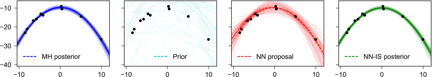
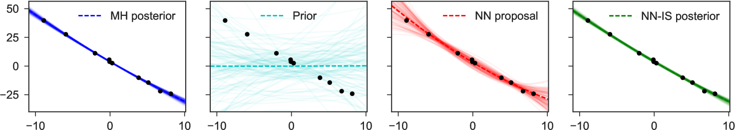
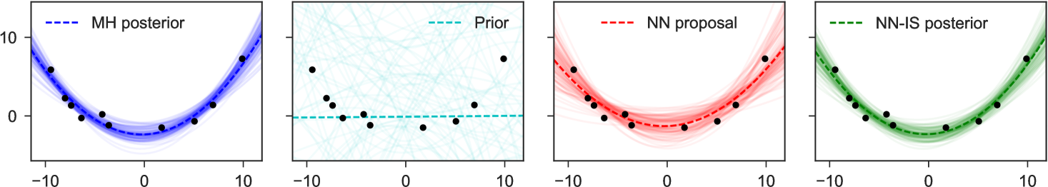
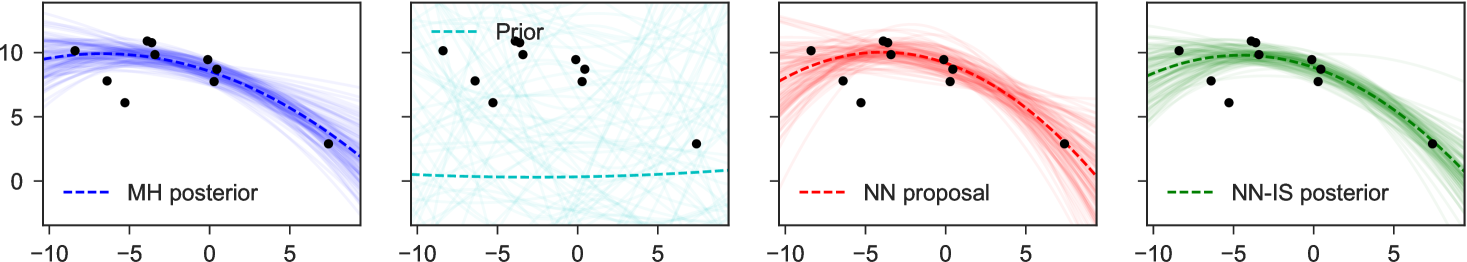
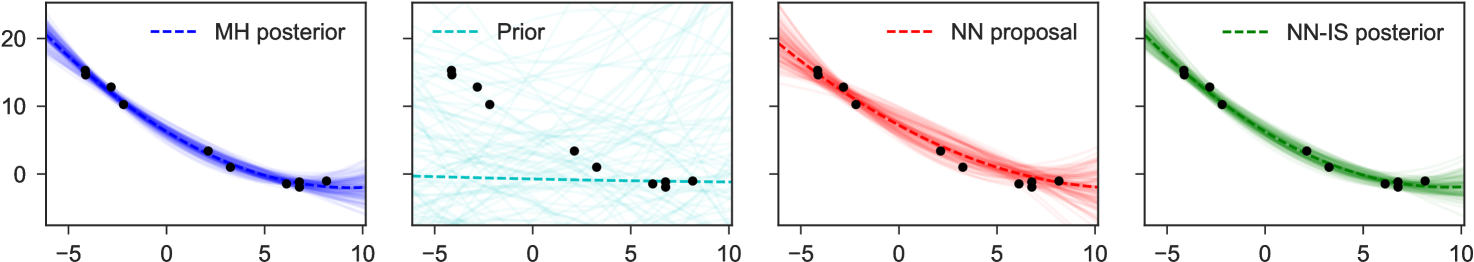
To illustrate the basic method for inverting factors, we consider a non-conjugate polynomial regression model, with global-only latent variables. The graphical model, its inversion, and the neural network structure are shown in Figure 1. Here we place a Laplace prior on the regression weights, and have Student-t likelihoods, giving us

for fixed $\nu=4,\epsilon=1$, and $z_{n}\in(-10,10)$ uniformly. The goal is to estimate the posterior distribution of weights for the constant, linear, and quadratic terms, given any possible collected dataset $\{z_{n},t_{n}\}_{n=1}^{N}$. In the notation of the preceding sections, we have latent variables $\boldsymbol{\mathbf{x}}\equiv\{w_{0},w_{1},w_{2}\}$ and observed variables $\boldsymbol{\mathbf{y}}\equiv\{z_{n},t_{n}\}_{n=1}^{N}$.

Note particularly that although the original graphical model which expressed $p(\boldsymbol{\mathbf{y}}|\boldsymbol{\mathbf{x}})p(\boldsymbol{\mathbf{x}})$ factorizes into products over $y_{n}$ which are conditionally independent given $\boldsymbol{\mathbf{x}}$, in the inverse model $\tilde{p}(\boldsymbol{\mathbf{x}}|\boldsymbol{\mathbf{y}})$ due to the explaining-away phenomenon all latent variables depend on all others: there are no latent variables which can be $d$-separated from the observed $\boldsymbol{\mathbf{y}}$, and all latent variables share $\boldsymbol{\mathbf{y}}$ as parents. This means we fit as proposal only a single joint density $q(w_{0:2}|z_{1:N},t_{1:N})$. Examples of representative output from this network are shown in Figure 4. The trained network used here 300 hidden units in each of two hidden layers, and a mixture of 3 Gaussians as each output.

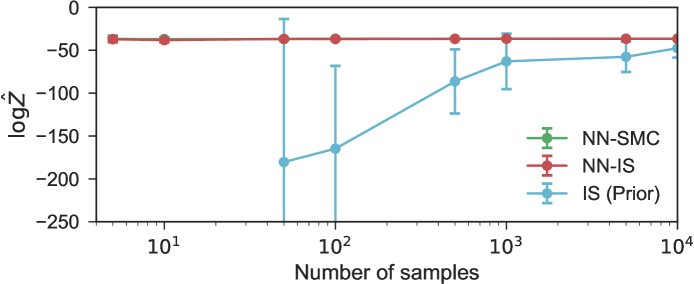
Consider as a new example a representative multilevel model where exact inference is intractable, a Poisson model for estimating failure rates of power plant pumps (George et al.,, 1993). Given $N$ power plant pumps, each having operated for $t_{n}$ thousands of hours, we see $x_{n}$ failures, following

The graphical model, an inverse factorization, and the neural network structure are shown in Figure 2. To generating synthetic training data, $t_{n}$ are sampled iid from an exponential distribution with mean 50.

The repeated structure in the inverse factorization of this model allows us to learn a single inverse factor to represent the distribution $\tilde{p}(\theta_{n}|t_{n},y_{n})$ across all $n$. This yields a far simpler learning problem than were we forced to fit all of $\tilde{p}(\theta_{1:N}|t_{1:N},y_{1:N})$ jointly. Further, the repeated structure allows us to use a divide-and-conquer SMC algorithm (Lindsten et al.,, 2014) which works particularly efficiently on this model. Each of the $N$ replicated structures are sampled in parallel with independent particle sets, weighted locally, and resampled; once all $\theta_{n}$ are sampled, we end by sampling $\alpha$ and $\beta$ jointly, which need both be included in order to evaluate the final terms in the joint target density. We stress that there is no obvious baseline proposal density to use for a divide-and-conquer SMC algorithm, as neither the marginal prior nor posterior distributions over $\theta_{n}$ are available in closed form. Any usage of this algorithm requires manual specification of some proposal $q(\theta_{n})$.

We test our proposals on the actual power pump failure data analyzed in George et al., (1993). The relative convergence speeds of marginal likelihood estimators from importance sampling from prior and neural network proposals, and SMC with neural network proposals, are shown in Figure 5. To capture the wide tails of the broad gamma distributions, we use a mixture of 10 Gaussians here at each output node, and 500 hidden units in each of two hidden layers.

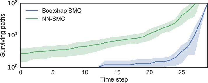
Proposals can also be learned to approximate the optimal filtering distribution in models for sequential data; we demonstrate here on a factorial hidden Markov model (Ghahramani and Jordan,, 1997), where each time step has a combinatorial latent space. The additive model we consider is inspired by the model studied in Kolter and Jaakkola, (2012) for disaggregation of household energy usage; effective inference in this model is a subject of continued research. Some number of devices $D$ are either in an active state, in which case each device $i$ consumes $\mu^{i}$ units of energy, or it is off, in which case it consumes no energy. At each time step we receive a noisy observation of the total amount of energy consumed, summed across all devices. This model, whose graphical model structure is shown in Figure 3, can be represented as

where $\theta^{i}$ represents the prior probability of devices switching on or off at each time increment. We design a synthetic example with $D=20$, meaning each time step has $2^{20}\approx 100,000$ possible discrete states; the parameters $\mu^{d}$ are spread out from 30 to 500, with $\sigma=20$. Each individual device has an initial probability $0.1$ of being activated at $t=1$, switching state at subsequent $t$ with probability $0.05$.

As different combinations of devices can yield identical total energy usage it is impossible to disambiguate between different combinations of active devices from a single observation, meaning any successful inference algorithm must attempt to mix across many disconnected modes over time to preserve the multiple possible explanations. The effect of the learned proposals on the overall number of surviving particles is shown in Figure 6. Our proposal model uses $D$ Bernoulli outputs in a 4-layer network, with 300 units per hidden layer; it takes as input the $D$ latent states at the previous time $t-1$, as well as the current observation $y_{t}$.

References

- Bengio and Bengio, (1999) Bengio, Y. and Bengio, S. (1999). Modeling high-dimensional discrete data with multi-layer neural networks. In Advances in Neural Information Processing Systems, volume 99, pages 400–406.
- Bishop, (1994) Bishop, C. M. (1994). Mixture density networks. Technical report.
- Cappé et al., (2008) Cappé, O., Douc, R., Guillin, A., Marin, J.-M., and Robert, C. P. (2008). Adaptive importance sampling in general mixture classes. Statistics and Computing, 18(4):447–459.
- Cornebise et al., (2008) Cornebise, J., Moulines, É., and Olsson, J. (2008). Adaptive methods for sequential importance sampling with application to state space models. Statistics and Computing, 18:461–480.
- Cornebise et al., (2014) Cornebise, J., Moulines, É., and Olsson, J. (2014). Adaptive sequential Monte Carlo by means of mixture of experts. Statistics and Computing, 24:317–337.
- Del Moral and Murray, (2015) Del Moral, P. and Murray, L. M. (2015). Sequential Monte Carlo with highly informative observations. SIAM/ASA Journal on Uncertainty Quantification, 3(1):969–997.
- Douc et al., (2005) Douc, R., Cappé, O., and Moulines, E. (2005). Comparison of resampling schemes for particle filtering. In In 4th International Symposium on Image and Signal Processing and Analysis (ISPA), pages 64–69.
- Doucet et al., (2001) Doucet, A., De Freitas, N., Gordon, N., et al. (2001). Sequential Monte Carlo methods in practice. Springer New York.
- Doucet et al., (2000) Doucet, A., Godsill, S., and Andrieu, C. (2000). On sequential Monte Carlo sampling methods for Bayesian filtering. Statistics and computing, 10(3):197–208.
- George et al., (1993) George, E. I., Makov, U., and Smith, A. (1993). Conjugate likelihood distributions. Scandinavian Journal of Statistics, pages 147–156.
- Germain et al., (2015) Germain, M., Gregor, K., Murray, I., and Larochelle, H. (2015). MADE: masked autoencoder for distribution estimation. In Proceedings of the 32nd International Conference on Machine Learning, ICML 2015, pages 881–889.
- Gershman and Goodman, (2014) Gershman, S. J. and Goodman, N. D. (2014). Amortized inference in probabilistic reasoning. In Proceedings of the Thirty-Sixth Annual Conference of the Cognitive Science Society.
- Ghahramani and Jordan, (1997) Ghahramani, Z. and Jordan, M. I. (1997). Factorial hidden Markov models. Machine learning, 29(2-3):245–273.
- Gordon et al., (1993) Gordon, N. J., Salmond, D. J., and Smith, A. F. (1993). Novel approach to nonlinear/non-Gaussian Bayesian state estimation. IEE Proceedings F (Radar and Signal Processing), 140(2):107–113.
- Gu et al., (2015) Gu, S., Ghahramani, Z., and Turner, R. E. (2015). Neural adaptive sequential Monte Carlo. In Advances in Neural Information Processing Systems 28.
- Heess et al., (2013) Heess, N., Tarlow, D., and Winn, J. (2013). Learning to pass expectation propagation messages. In Advances in Neural Information Processing Systems 26, pages 3219–3227.
- Hinton et al., (1995) Hinton, G. E., Dayan, P., Frey, B. J., and Neal, R. M. (1995). The “wake-sleep” algorithm for unsupervised neural networks. Science, 268(5214):1158–1161.
- Jampani et al., (2015) Jampani, V., Nowozin, S., Loper, M., and Gehler, P. V. (2015). The informed sampler: A discriminative approach to Bayesian inference in generative computer vision models. Computer Vision and Image Understanding, 136:32–44.
- Jordan et al., (1999) Jordan, M. I., Ghahramani, Z., Jaakkola, T. S., and Saul, L. K. (1999). An introduction to variational methods for graphical models. Machine learning, 37(2):183–233.
- Jun and Bouchard-Côté, (2014) Jun, S.-H. and Bouchard-Côté, A. (2014). Memory (and time) efficient sequential Monte Carlo. In Proceedings of the 31st international conference on Machine learning, pages 514–522.
- Kingma and Ba, (2015) Kingma, D. and Ba, J. (2015). Adam: A method for stochastic optimization. In Proceedings of the International Conference on Learning Representations (ICLR).
- Kingma and Welling, (2014) Kingma, D. P. and Welling, M. (2014). Auto-encoding variational Bayes. In Proceedings of the International Conference on Learning Representations (ICLR).
- Kolter and Jaakkola, (2012) Kolter, J. Z. and Jaakkola, T. (2012). Approximate inference in additive factorial HMMs with application to energy disaggregation. In International conference on artificial intelligence and statistics, pages 1472–1482.
- Kulkarni et al., (2015) Kulkarni, T. D., Kohli, P., Tenenbaum, J. B., and Mansinghka, V. K. (2015). Picture: a probabilistic programming language for scene perception. In Proceedings of the IEEE Conference on Computer Vision and Pattern Recognition.
- Larochelle and Murray, (2011) Larochelle, H. and Murray, I. (2011). The neural autoregressive distribution estimator. In International Conference on Artificial Intelligence and Statistics, pages 29–37.
- Lindsten et al., (2014) Lindsten, F., Johansen, A. M., Naesseth, C. A., Kirkpatrick, B., Schön, T. B., Aston, J., and Bouchard-Côté, A. (2014). Divide-and-conquer with sequential Monte Carlo. arXiv preprint arXiv:1406.4993.
- Minka, (2005) Minka, T. (2005). Divergence measures and message passing. Technical report, Microsoft Research.
- Murray et al., (2014) Murray, L. M., Lee, A., and Jacob, P. E. (2014). Parallel resampling in the particle filter. arXiv preprint arXiv:1301.4019.
- Naesseth et al., (2014) Naesseth, C. A., Lindsten, F., and Schön, T. B. (2014). Sequential Monte Carlo for graphical models. In Advances in Neural Information Processing Systems 27.
- Naesseth et al., (2015) Naesseth, C. A., Lindsten, F., and Schön, T. B. (2015). Towards automated sequential Monte Carlo for probabilistic Graphical Models. In NIPS Workshop on Black Box Learning and Inference.
- Paige et al., (2014) Paige, B., Wood, F., Doucet, A., and Teh, Y. W. (2014). Asynchronous anytime sequential Monte Carlo. In Advances in Neural Information Processing Systems 27, pages 3410–3418.
- Pearl and Russell, (1998) Pearl, J. and Russell, S. (1998). Bayesian networks. Computer Science Department, University of California.
- Pitt and Shephard, (1999) Pitt, M. K. and Shephard, N. (1999). Filtering via simulation: auxiliary particle filter. Journal of the American Statistical Association, 94:590–599.
- Ritchie et al., (2015) Ritchie, D., Mildenhall, B., Goodman, N. D., and Hanrahan, P. (2015). Controlling procedural modeling programs with stochastically-ordered sequential Monte Carlo. ACM Transactions on Graphics (TOG), 34(4):105.
- Stuhlmüller et al., (2013) Stuhlmüller, A., Taylor, J., and Goodman, N. (2013). Learning stochastic inverses. In Advances in Neural Information Processing Systems 26, pages 3048–3056.
- Todeschini et al., (2014) Todeschini, A., Caron, F., Fuentes, M., Legrand, P., and Del Moral, P. (2014). Biips: software for Bayesian inference with interacting particle systems. arXiv preprint arXiv:1412.3779.
- Uria et al., (2013) Uria, B., Murray, I., and Larochelle, H. (2013). RNADE: The real-valued neural autoregressive density-estimator. In Advances in Neural Information Processing Systems, pages 2175–2183.
- Van Der Merwe et al., (2000) Van Der Merwe, R., Doucet, A., De Freitas, N., and Wan, E. (2000). The unscented particle filter. In Advances in Neural Information Processing Systems, pages 584–590.
- Wood et al., (2014) Wood, F., van de Meent, J. W., and Mansinghka, V. (2014). A new approach to probabilistic programming inference. In Proceedings of the 17th International conference on Artificial Intelligence and Statistics.