Inferential Wasserstein Generative Adversarial Networks
Abstract
Generative Adversarial Networks (GANs) have been impactful on many problems and applications but suffer from unstable training. The Wasserstein GAN (WGAN) leverages the Wasserstein distance to avoid the caveats in the minmax two-player training of GANs but has other defects such as mode collapse and lack of metric to detect the convergence. We introduce a novel inferential Wasserstein GAN (iWGAN) model, which is a principled framework to fuse auto-encoders and WGANs. The iWGAN model jointly learns an encoder network and a generator network motivated by the iterative primal dual optimization process. The encoder network maps the observed samples to the latent space and the generator network maps the samples from the latent space to the data space. We establish the generalization error bound of the iWGAN to theoretically justify its performance. We further provide a rigorous probabilistic interpretation of our model under the framework of maximum likelihood estimation. The iWGAN, with a clear stopping criteria, has many advantages over other autoencoder GANs. The empirical experiments show that the iWGAN greatly mitigates the symptom of mode collapse, speeds up the convergence, and is able to provide a measurement of quality check for each individual sample. We illustrate the ability of the iWGAN by obtaining competitive and stable performances for benchmark datasets.
Keywords: generalization error, generative adversarial networks, latent variable models, primal dual optimization, Wasserstein distance.
1 Introduction
One of the goals of generative modeling is to match the model distribution with parameters to the true data distribution for a random variable . For latent variable models, the data point is generated from a latent variable through a conditional distribution . Here denotes the support for and denotes the support for . In this paper, we consider models with . There has been a surge of research on deep generative networks in recent years and the literature is too vast to summarize here (Kingma and Welling, 2014; Goodfellow et al., 2014; Li et al., 2015; Gao et al., 2020; Qiu and Wang, 2020). These models have provided a powerful framework for modeling complex high dimensional datasets.
We start introducing two main approaches for generative modeling. The first one is called variational auto-encoders (VAEs) (Kingma and Welling, 2014), which use variational inference (Blei et al., 2017) to learn a model by maximizing the lower bound of the likelihood function. Specifically, let the latent variable be drawn from a prior and the data have a likelihood that is conditioned on . Unfortunately obtaining the marginal distribution of requires computing an intractable integral . Variational inference approximates the posterior by a family of distribution with the parameter . The objective is to maximize the lower bound of the log-likelihood function known as the evidence lower bound (ELBO). The ELBO is given by
Note that the difference between the log-likelihood and the ELBO is the Kullback-Leibler divergence between and the true posterior . Usually is a normal density where both the conditional mean and the conditional covariance are modeled by deep neural networks (DNNs), so that the first term of the ELBO can be approximated efficiently by Monte Carlo methods and the second term can be calculated explicitly. Therefore, the ELBO allows us to do approximate posterior inference with tractable computation. VAEs have elegant theoretical foundations but the drawback is that they tend to produce blurry images. The second approach is called generative adversarial networks (GANs) (Goodfellow et al., 2014), which learn a model by using a powerful discriminator to distinguish between real data samples and generative data samples. Specifically, we define a generator and a discriminator . The generator and discriminator play a two-player minimax game by being alternatively updated, such that the generator tries to produce real-looking images and the discriminator tries to distinguish between generated images and observed images. The GAN objective can be written as , where
GANs produce more visually realistic images but suffer from the unstable training and the mode collapse problem. Although there are many variants of generative models trying to take advantages of both VAEs and GANs (Tolstikhin et al., 2018; Rosca et al., 2017), to the best of our knowledge, the model which provides a unifying framework combining the best of VAEs and GANs in a principled way is yet to be discovered.
1.1 Related work
In this section, we provide a brief introduction of different variants of generative models.
Wasserstein GAN. The Wasserstein GAN (WGAN) (Arjovsky et al., 2017) is an extension to the GAN that improves the stability of the training by introducing a new loss function motivated from the Waseerstein distance between two probability measures (Villani, 2008). Let denote the generative model distribution through the generator and the latent variable . Both the vanilla GAN (Goodfellow et al., 2014) and the WGAN can be viewed as minimizing certain divergence between the data distribution and the generative distribution . For example, the Jensen-Shannon (JS) divergence is implicitly used in vanilla GANs (Goodfellow et al., 2014), while the -Wasserstein distance is employed in WGANs. Empirical experiments suggest that the Wasserstein distance is a more sensible measure to differentiate probability measures supported in low-dimensional manifold. In terms of training, it turns out that it is hard or even impossible to compute these standard divergences in probability, especially when is unknown and is parameterized by DNNs. Instead, the training of WGANs is to study its dual problem because of the elegant form of Kantorovich-Rubinstein duality (Villani, 2008).
Autoencoder GANs. The main difference between autoencoder GANs and standard GANs is that, besides the generator , there is an encoder which maps the data points into the latent space. This deterministic encoder is to approximate the conditional distribution of the latent variable given the data point . Larsen et al. (2016) first introduced the VAE-GAN, which is a hybrid of VAEs and GANs and uses a GAN discriminator to replace a VAE’s decoder to learn the loss function. For both the Adversarially Learned Inference (ALI) (Dumoulin et al., 2017) and the Bidirectional Generative Adversarial Network (BiGAN) (Donahue et al., 2017), the objective is to match two joint distributions, and , under the framework of vanilla GANs. When the algorithm achieves equilibrium, these two joint distributions roughly match. It is expected to obtain more meaningful latent codes by , and this should improve the quality of the generator as well. For other VAE-GAN variants, please see Rosca et al. (2017); Mescheder et al. (2017); Hu et al. (2018); Ulyanov et al. (2018).
Energy-Based GANs. Energy-based Generative Adversarial Networks (EBGANs) (Zhao et al., 2017) view the discriminator as an energy function that attributes low energies to the regions near the data manifold and higher energies to other regions, and the generator as being trained to produce contrastive samples with minimal energies. Han et al. (2019) presented the joint training of generator model, energy-based model, and inference model, which introduces a new objective function called divergence triangle that makes the processes of sampling, inference, energy evaluation readily available without the need for costly Markov chain Monte Carlo methods.
Duality in GANs. Regarding the optimization perspectives of GANs, (Chen et al., 2018; Zhao et al., 2018) studied duality-based methods for improving algorithm performance for training. Farnia and Tse (2018) developed a convex duality framework to address the case when the discriminator is constrained into a smaller class. Grnarova et al. (2018) developed an evaluation metric to detect the non-convergence behavior of vanilla GANs, which is the duality gap defined as the difference between the primal and the dual objective functions.
1.2 Our Contributions
Although there are many interesting works on autoencoder GANs, it remains unclear what the principles are underlying the fusion of auto-encoders and GANs. For example, do there even exist these two mappings, the encoder and the decoder , for any high-dimensional random variable , such that has the same distribution as and has the same distribution as ? Is there any probabilistic interpretation such as the maximum likelihood principle on autoencoder GANs? What is the generalization performance of autoencoder GANs? In this paper, we introduce inferential WGANs (iWGANs), which provide satisfying answers for these questions. We will mainly focus on the 1-Wasserstein distance, instead of the Kullback-Leibler divergence. We borrow the strength from both the primal and the dual problems and demonstrate the synergistic effect between these two optimizations. The encoder component turns out to be a natural consequence from our algorithm. The iWGAN learns both an encoder and a decoder simultaneously. We prove the existence of meaningful encoder and decoder, establish an equivalence between the WGAN and iWGAN, and develop the generalization error bound for the iWGAN. Furthermore, the iWGAN has a natural probabilistic interpretation under the maximum likelihood principle. Our learning algorithm is equivalent to the maximum likelihood estimation motivated from the variational approach when our model is defined as an energy-based model based on an autoencoder. As a byproduct, this interpretation allows us to perform the quality check at the individual sample level. In addition, we demonstrate the natural use of the duality gap as a measure of convergence for the iWGAN, and show its effectiveness for various numerical settings. Our experiments do not experience any mode collapse problem.
The rest of the paper is organized as follows. Section 2 presents the new iWGAN framework, and its extension to general inferential f-GANs. Section 3 establishes the generalization error bound and introduces the algorithm for the iWGAN. The probabilistic interpretation and the connection with the maximum likelihood estimation are introduced in Section 4. Extensive numerical experiments are demonstrated in Section 5 to show the advantages of the iWGAN framework. Proofs of theorems and additional numerical results are provided in the Appendix.
2 The iWGAN Model
The autoencoder generative model consists of two parts: an encoder and a generator . The encoder maps a data sample to a latent variable , and the generator takes a latent variable to produce a sample . In general, the autoencoder generative model should satisfy the following three conditions simultaneously: (a) The generator can generate images which have a similar distribution with observed images, i.e., the distribution of is similar to that of ; (b) The encoder can produce meaningful encodings in the latent space, i.e., has a similar distribution with ; (c) The reconstruction errors of this model based on these meaningful encodings are small, i.e., the difference between and is small.
We emphasize that the benefit of using an autoencoder is to encourage the model to better represent all the data it is trained with, so that it discourages mode collapse. We first show that, for any distribution residing on a compact smooth Riemannian manifold 111A smooth manifold is a manifold with a atlas on . A atlas is a collection of charts such that covers , and for all and , the transition map is a map. Here is an open subset of . For any point , let be the tangent space of at . A Riemannian metric assigns to each a positive definite inner product , along with which comes a norm defined by . The smooth manifold endowed with this metric is called a smooth Reimannian manifold., there always exists an encoder which guarantees meaningful encodings and exists a generator which generates samples with the same distribution as data points by using these meaningful codes.
Theorem 1.
Consider a continuous random variable , where is a -dimensional compact smooth Riemannian manifold. Then, there exist two mappings and , with , such that follows a multivariate normal distribution with zero mean and identity covariance matrix and is an identity mapping, i.e., .
Theorem 1 is a natural consequence of the Nash embedding theorem (Nash, 1956; Günther, 1991) and the probability integral transformation (Rosenblatt, 1952). In Theorem 1, we have proved the existence of and , however, learning and from the data points is still a challenging task. Consider a general -GAN model (Nowozin et al., 2016). Let be a convex function with . The -GAN defines the -divergence between the data distribution and the generative model distribution for the generator as:
where is the convex conjugate of and is a class of functions whose output range is the domain of . When is approximated by a DNN, its output range can be achieved by choosing an appropriate activation function specific to the f-divergence used. For example, if , then the corresponding convex conjugate . To satisfy the above condition, we select the output activation function of the DNN to be such that the -GAN can recover the original vanilla GAN (Goodfellow et al., 2014). If when and otherwise, we have . With the property that is 1-Lipschitz function class, the -GAN turns to be the WGAN.
For ease of presentation, we illustrate our methodology by mainly focusing on the Wasserstein distance and the inferential WGAN (iWGAN) model. The extension to general inferential f-GANs (ifGANs) is straightforward and will be presented in Section 2.3.
2.1 iWGAN
Recall that the -Wasserstein distance between and is defined as
| (1) |
where represents the -norm and is the set of all joint distributions of with marginal measures and , respectively. The main difficulty in (1) is to find the optimal coupling , and this is a constrained optimization because the joint distribution needs to match these two marginal distributions and .
Based on the Kantorovich-Rubinstein duality (Villani, 2008), the WGAN studies the -Wasserstein distance (1) through its dual format
| (2) |
where is the set of all bounded -Lipschitz functions. This is also a constrained optimization due to the Lipschitz constraint on such that for all . Weight clipping (Arjovsky et al., 2017) and gradient penalty (Gulrajani et al., 2017) have been used to satisfy the constraint of Lipschitz continuity. Arjovsky et al. (2017) used a clipping parameter to clamp each weight parameter to a fixed interval after each gradient update is set. However, this method is very sensitive to the choice of clipping parameter . Instead, Gulrajani et al. (2017) introduced a gradient penalty, , in the loss function to enforce the Lipschitz constraint, where is sampled uniformly along straight lines between pairs of points sampled from and . This is motivated by the fact that the optimal critic contains straight lines with gradient norm connecting coupled points from and . The experiment of (Arjovsky et al., 2017) showed that the WGAN can avoid the problem of gradient vanishment. However, the WGAN does not produce meaningful encodings and many experiments still display the problem of mode collapse (Arjovsky et al., 2017; Gulrajani et al., 2017).
On the other hand, the Wasserstein Autoencoder (WAE) (Tolstikhin et al., 2018), after introducing an encoder to approximate the conditional distribution of given , minimizes the reconstruction error , where is a set of encoder mappings whose elements satisfies . The penalty, such as , is added to the objective to satisfy this constraint, where is an arbitrary divergence between and . The WAE can produce meaningful encodings and has controlled reconstruction error. However, the WAE defines a generative model in an implicit way and does not model the generator through with directly.
To take the advantages of both the WGAN and WAE, we propose a new autoencoder GAN model, called the iWGAN, which defines the divergence between and by
| (3) |
Our goal is to find the tuple which minimizes . The motivation and explanation of this objective function are provided in Section 2.2 in detail. The term can be treated as the autoencoder reconstruction error as well as a loss to match the distributions between and . We note that the -norm has been used for the reconstruction term by the -GAN (Rosca et al., 2017) and CycleGAN (Zhu et al., 2017). Another term can be treated as a loss for the generator as well as a loss to match the distribution between and . We emphasize that this term is different with the objective function of the WGAN in (2). The properties of (3) will be discussed in Theorem 2, and the primal and dual explanation of (3) will be presented in Section 2.2.
Furthermore, it is challenging for practitioners to determine when to stop training GANs. Most of the GAN algorithms do not provide any explicit standard for the convergence of the model. However, the measure of convergence for the iWGAN becomes very natural and we use the duality gap as the measure. For a given tuple , the duality gap is defined as
| (4) |
where is
In practice, the function spaces , , and are modeled by spaces containing deep neural networks with specific architectures. The architecture hyperparameters usually include number of channels, number of layers, and width of each layer. The architectures for our numerical experiments are provided in the appendix. We assume that these network spaces are large enough to include the true encoder , generator , and the optimal discriminator in (2). This is not a strong assumption due to the universal approximation theorem of DNNs (Hornik, 1991).
Theorem 2.
(a). The iWGAN objective (3) is equivalent to
| (5) |
Therefore, .
If there exists a such that has the same distribution with , then .
(b). Let be a fixed solution.
Then
Moreover, if outputs the same distribution as and outputs the same distribution as , both the duality gap and are zeros and for .
According to Theorem 2, the iWGAN objective is in general the upper bound of . However, this upper bound is tight. When the space includes a special encoder such that has the same distribution as , the iWGAN objective is exactly the same as . Theorem 2 also provides an appealing property from a practical point of view. The values of both the duality gap and give us a natural criteria to justify the algorithm convergence.
2.2 A Primal-Dual Explanation
We explain the iWGAN objective function (3) from the view of primal and dual problems. Note that both the primal problem (1) and the dual problem (2) are constrained optimization problems. First, for the primal problem (1), two constraints on are for all , and for all . Recall that the primal variable for the dual problem (2) is also a dual variable for the primal problem (1). From the Lagrange multiplier perspective, we can write the primal problem (1) as
where we use the encoder to approximate the conditional distribution of given , and the Lagrange multipliers for two constraints are and respectively. Second, for the dual problem (2), the -Lipschitz constraint on is for all and . Recall that the primal variable for the primal problem (1) is also a dual variable for the dual problem (2). Similarly, we can write the dual problem (2) as
where the Lagrange multiplier for the -Lipschitz constraint is . When we solve primal and dual problems iteratively, this turns out to be exactly the same as our iWGAN algorithm.
2.3 Extension to f-GANs
This framework can be easily extended to other types of GANs. Assume that is the 1-Lipschitz function class. We extend the iWGAN framework to the inferential f-GAN (ifGAN) framework. Define the ifGAN objective function as follows:
|
. |
(6) |
Following this definition, we have
We show . This is because
This indicates that the ifGAN objective (6) is an upper bound of the f-GAN objective.
3 Generalization Error Bound and the Algorithm
Suppose that we observe samples . In practice, we minimize the empirical version, denoted by , of to learn both the encoder and the generator, where,
| (7) |
Here denotes the empirical average on the observed data and denotes the empirical average on a random sample of standard normal random variables. Before we present the details of the algorithm, we first establish the generalization error bound for the iWGAN in this section.
In the context of supervised learning, generalization error is defined as the gap between the empirical risk and the expected risk. The empirical risk is corresponding to the training error, and the expected risk is corresponding to the testing error. Mathematically, the difference between the expected risk and the empirical risk, i.e. the generalization error, is a measure of how accurately an algorithm is able to predict outcome values for previously unseen data. However, in the context of GANs, neither the training error nor the test error is well defined. But we can define the generalization error in a similar way. Explicitly, we define the “training error” as in (7), which is minimized based on observed samples. Define the “test error” as in (1), which is the true 1-Wasserstein distance between and . The generalization error for the iWGAN is defined as the gap between these two “errors”. In other words, for an iWGAN model with the parameter , the generalization error is defined as . For discussions of generalization performance of classical GANs, see Arora et al. (2017) and Jiang et al. (2019).
Theorem 3.
Given a generator , and samples from , with probability at least for any , we have
| (8) |
where is the empirical Rademacher complexity of the 1-Lipschitz function set , in which is the Rademacher variable.
For a fixed generator , Theorem 3 holds uniformly for any discriminator . It indicates that the 1-Wasserstein distance between and can be dominantly upper bounded by the empirical and Rademacher complexity of . Since for any , the capacity of determines the value of . In learning theory, Rademacher complexity, named after Hans Rademacher, measures richness of a class of real-valued functions with respect to a probability distribution. There are several existing results on the empirical Rademacher complexity of neural networks. For example, when is a set of 1-Lipschitz neural networks, we can apply the conclusion from Bartlett et al. (2017) to , which produces an upper bound scaling as . Here denotes the depth of network . Similar upper bound with an order of can be obtained by utilizing the results from Li et al. (2019), where is the width of the network.
Next, we introduce the details of the algorithm. Our target is to solve the following optimization problem:
|
, |
(9) |
where and are regularization terms for and respectively. We approximate by three neural networks with pre-specified architectures.
Since is assumed to be 1-Lipschitz, we adopt the gradient penalty defined as in (Gulrajani et al., 2017) to enforce the 1-Lipschitz constraint on . Furthermore, since we expect follows approximately standard normal, we use the maximum mean discrepancy (MMD) penalty (Gretton et al., 2012), denoted by , to enforce to converge to . In particular,
where is set to be the Gaussian radial kernel function .
We have adopted the stochastic gradient descent algorithm called the ADAM (Kingma and Ba, 2015) to estimate the unknown parameters in neural networks. The ADAM is an algorithm for first-order gradient-based optimization of stochastic objection functions, based on adaptive estimates of lower-order moments. Given the current tuple at the th iteration, we sample a batch of observations , latent variable , and . Then we construct , , for computing the gradient penalty. Let and . We can evaluate the gradient with respect to the parameters in , which is denoted by
Then we can update by the ADAM using this gradient. Similarly, we can evaluate the gradient with respect to the parameters in and , which is denoted by
Then we can update by the ADAM using this gradient. The stopping criteria are both the DualGap in (4) and the objective function are less than pre-specified error tolerances and , respectively. Specifically, based on the definition of the duality gap in (4), we approximate DualGap by the difference between and The optimization (9) consists of two tuning parameters and . We pre-specify some values for and and select the optimal tuning parameters by grid search using cross validation. The details of the algorithm are presented in Algorithm 1.
4 Probabilistic Interpretation and the MLE
The iWGAN has proposed an efficient framework to stably and automatically estimate both the encoder and the generator. In this section, we provide a probabilistic interpretation of the iWGAN under the framework of maximum likelihood estimation.
Maximum likelihood estimator (MLE) is a fundamental statistical framework for learning models from data. However, for complex models, MLE can be computationally prohibitive due to the intractable normalization constant. MCMC has been used to approximate the intractable likelihood function but do not work efficiently in practice, since running MCMC till convergence to obtain a sample can be computationally expensive. For example, to reduce the computational complexity, Hinton (2002) proposed a simple and fast algorithm, called the contrastive divergence (CD). The basic idea of CD is to truncate MCMC at the -th step, where is a fixed integer as small as one. The simplicity and computational efficiency of CD makes it widely used in many popular energy-based models. However, the success of CD also raised a lot of questions regarding its convergence property. Both theoretical and empirical results show that CD in general does not converge to a local minimum of the likelihood function (Carreira-Perpinan and Hinton, 2005; Qiu et al., 2020), and diverges even in some simple models (Schulz et al., 2010; Fischer and Igel, 2010). The iWGAN can be treated as an adaptive method for the MLE training, which not only provides computational advantages but also allows us to generate more realistic-looking images. Furthermore, this probabilistic interpretation enables other novel applications such as image quality checking and outlier detection.
Let denote the image. Define the density of by an energy-based model based on an autoencoder (Gu and Zhu, 2001; Zhao et al., 2017; Berthelot et al., 2017):
| (10) |
where
and is the unknown parameter and is the log normalization constant. The major difficulty for the likelihood inference is due to the intractable function . Suppose that we have the observed data . The log-likelihood function of is , whose gradient is
| (11) |
where denotes the empirical average on the observed data and denotes the expectation under model . The key computational obstacle lies in the approximations of the model expectation .
To address this problem, we can rewrite the log-likelihood function by introducing a variational distribution . This leads to
| (12) |
where denotes the entropy of and the inequality is due to Jensens’s inequality. Equation (4) provides an upper bound for the log-likelihood function. We expect to choose so that (4) is closer to the log-likelihood function, and then maximize (4) as a surrogate for maximizing log-likelihood. We choose and define the surrogate log-likelihood as
| (13) |
Theorem 4.
(a). For any , we have . In addition, .
(b). Consider the following algorithm and the th iteration is obtained by , for . If as , then is the MLE.
Theorem 4 shows that, if we maximize the surrogate log-likelihood function and the algorithm converges, the solution is exactly the same as the MLE. The additional identity is the key to our algorithm to obtain the MLE, which is different with the ELBO in VAEs. The ELBO is in general not a tight lower bound of the log-likelihood function.
In terms of training, by Theorem 5.10 of Villani (2008), for any random variables and , there exists an optimal such that
| (14) |
for the optimal coupling which is the joint distribution of and . Therefore, there exists a such that
| (15) |
with probability one. Because needs to be learned as well, we approximate by a neural network with an unknown parameter . This amounts to using the following max-min objective
| (16) |
Note that, for the gradient update, the expectation in (16) is taken under the current estimated . Since we require to be a good generator and the distributions of is close the distribution , we replace by . Since an additional regularization is added to enforce to follow a normal distribution, we use the expectation under the data distribution to replace the second expectation of (16). This yields a gradient update for of form , where
| (17) |
A gradient update for is given by
| (18) |
The above iterative updating process is exactly the same as in Algorithm 1. Therefore, the training of the iWGAN is to seek the MLE. This probabilistic interpretation provides a novel alternative method to tackle problems with the intractable normalization constant in latent variable models. The MLE gradient update of decreases the energy of the training data and increases the dual objective. Compare with original GANs or WGANs, our method gives much faster convergence and simultaneously provides a higher quality generated images.
The probabilistic modeling opens a door for many interesting applications. Next, we present a completely new approach for determining a highest density region (HDR) estimate for the distribution of . What makes HDR distinct from other statistical methods is that it finds the smallest region, denoted by , in the high dimensional space with a given probability coverage , i.e., . We can use to assess each individual sample quality. Note that commonly used inception scores (IS) and Fréchet inception distances (FID) are to measure the whole sample quality, not at the individual sample level. More introductions of IS and FID are given in Appendix G. Let be the MLE. The density ratio at and is
The smaller the reconstruction error is, the larger the density value is. We can define the HDR for through the HDR for the reconstruction error , which is simple because it is a one-dimensional problem. Let be the HDR for . Then, . Here defines the corresponding region in the latent space, which can be used to generate better quality samples.
5 Experimental Results
The goal of our numerical experiments is to demonstrate that the iWGAN can achieve the following three objectives simultaneously: high-quality generative samples, meaningful latent codes, and small reconstruction errors. We also compare the iWGAN with other well-known GAN models such as the Wasserstein GAN with gradient penalty (WGAN-GP) (Gulrajani et al., 2017), the Wasserstein Autoencoder (WAE) (Tolstikhin et al., 2018), the Adversarial Learned Inference (ALI) (Dumoulin et al., 2017), and the CycleGAN (Zhu et al., 2017) to illustrate a competitive and stable performance for benchmark datasets.
5.1 Mixture of Gaussians
We first train our iWGAN model on three datasets from the mixture of Gaussians with an increasing difficulty shown in the Figure 1: a). RING: a mixture of 8 Gaussians with means and standard deviation , b). SPIRAL: a mixture of 20 Gaussians with means and standard deviation and c). GRID: a mixture of 25 Gaussians with means and standard deviation . As the true data distributions are known, this setting allows for tracking of convergence and mode dropping.


Duality gap and convergence. We illustrate that as the duality gap converges to , our model converges to the generated samples from the true distribution. We keep track of the generated samples using and record the duality gap at each iteration to check the corresponding generated samples. We compare our method with the WGAN-GP and CycleGAN in Figure 2. All methods adopt the same structure, learning rate, number of critical steps, and other hyper-parameters.

Figure 2 shows that the iWGAN converges quickly in terms of both the duality gap and the true distributions learning. Duality gap has also been a good indicator of whether the model has generated the desired distribution. When comparing with the WGAN model, the iWGAN surpasses the performance of the WGAN-GP at very early stage and avoids the appearance of mode collapse. We have further tested the CycleGAN on these distributions. The CycleGAN objective function is the sum of two parts. The first part includes two vanilla GAN objectives (Goodfellow et al., 2014) to differentiate between and , and and . The second part is the cycle consistency loss given by , where is the -norm of a vector. Unfortunately, Figure 2 shows that the CycleGAN fails on all three distributions and experienced the mode collapse problem.


Latent space. We choose the latent distribution to be a 5-dimensional standard multivariate normal distribution . During the training each batch size is chosen to be 512. After training, the distribution of is expected to be close to the distribution of . To demonstrate the latent distribution visually, we plot the th compoment of , , against the th compoment of , , for all in Figure 3. We can tell that the joint distribution of any two dimensions of is close to a bivariate normal distribution.

Mode collapse. We investigate the mode collapse problem for the iWGAN. If we draw two random samples in the latent space , the interpolation, , , should fall around the mode to represent a reasonable sample. In Figure 4, we select , and do interpolations on two random samples. We repeat this procedure several times on 3 datasets as demonstrated in Figure 4. No matter where the interpolations start and end, the interpolations would fall around the modes other than the locations where true distribution has a low density. There may still be some samples that appears in the middle of two modes. This may be because the generator is not able to approximate a step function well.

Individual sample quality check. From the probability interpretation of the iWGAN, we naturally adopt the reconstruction error , or the quality score
as the metric of the quality of any individual sample. The larger the quality score is, the better quality the sample has. Figure 5 shows their quality scores for different samples. The quality scores of samples near the modes of the true distribution are close to 1, and become smaller as the sample draw is away from the modes. This indicates that the iWGAN converges and learns the distribution well, and the quality score is a reliable metric for the individual sample quality.
5.2 CelebA
We experimentally demonstrate our model’s ability on two well-known benchmark datasets, MNIST and CelebA. We present the performance of the iWGAN on CelebA in this section and the performance on MNIST in the Appendix. CelebA (CelebFaces Attributes Dataset) is a large-scale face attributes dataset with colored celebrity face images, which cover large pose variations and diverse people. This dataset is ideal for training models to generate synthetic images. The MNIST database (Modified National Institute of Standards and Technology database) is another large database of handwritten digits that is commonly used for training various image processing systems. The MNIST database contains grey images. CelebA is a more complex dataset than MNIST. The CelebA dataset is available at http://mmlab.ie.cuhk.edu.hk/projects/CelebA.html and the MNIST dataset is available at http://yann.lecun.com/exdb/mnist/.


.
The first result by the iWGAN on CelebA is shown in Figure 6(c). The dimension of the latent space is chosen to be . For each panel, Figure 6(c) respectively shows the generated samples from , the reconstructed samples from , and the latent space interpolation between two randomly chosen images. In particular, we perform latent space interpolations between CelebA validation set examples. We sample pairs of validation set examples and and project them into and by the encoder . We then linearly interpolate between and and pass the intermediate points through the decoder to plot the input-space interpolations. In addition, Figure 7 shows the first 8 dimensions of the latent space calculated by on CelebA. Figures 6(c) and 7 visually demonstrate that the iWGAN can simultaneously generate high quality samples, produce small reconstruction errors, and have meaningful latent codes. Figure 8 also displays images with high and low quality scores selected from CelebA. The images with low quality scores are quite different with other images in the dataset and these images usually contain lighter background with masks or glasses.


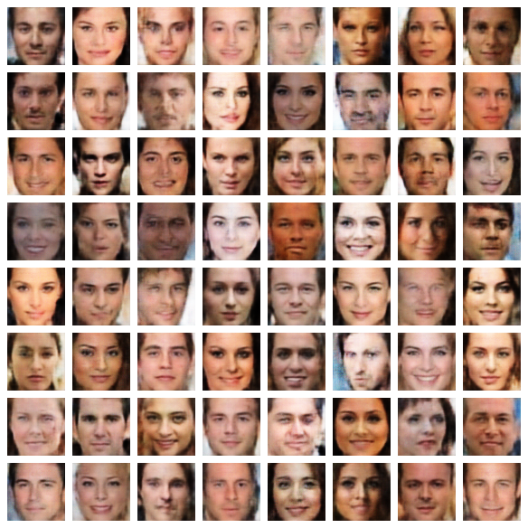


We compare the iWGAN, both visually and numerically, with the WGAN-GP, WAE, ALI, and CycleGAN. Figures 9(a)—9(e) display the random generated samples from the iWGAN, WGAN-GP, WAE, ALI, and CycleGAN, respectively. The generated faces by the iWGAN demonstrate higher qualities than other four methods. The top panel of Figure 10 shows the comparison between real images and reconstructed images among four methods, the iWGAN, WAE, ALI, and CycleGAN. Note that the WGAN-GP cannot provide reconstructed images since it does not produce the latent codes. The bottom panel of Figure 10 shows the interpolated images by the iWGAN, WAE, ALI, and CycleGAN.


We numerically compare these five methods, the iWGAN, ALI, WAE, CycleGAN, and WGAN-GP. Four performance measures are chosen, which are inception scores (IS), Fréchet inception distances (FID), reconstruction errors (RE), and maximum mean discrepancy (MMD) between encodings and standard normal random variables. The details of these comparison metrics are given in Appendix G. Proposed by Salimans et al. (2016), the IS involves using a pre-trained Inception v3 model to predict the class probabilities for each generated image. Higher scores are better, corresponding to a larger KL-divergence between the two distributions. The FID is proposed by Heusel et al. (2017) to improve the IS by actually comparing the statistics of generated samples to real samples. For the FID, the lower the better. However, as discussed in Barratt and Sharma (2018), IS is not a reliable metric for the wellness of generated samples. This is also consistent with our experiments. Although the WAE delivers the best inception scores among five methods, the WAE also has the worst FID scores. The generated samples (Figure 9(c)) show that the WAE is not the best generative model compared with other four methods. Furthermore, The reconstruction error (RE) is used to measure if the method has generated meaningful latent encodings. Smaller reconstruction errors indicate a more meaningful latent space which can be decoded into the original samples. The MMD is used to measure the difference between distribution of latent encodings and standard normal random variables. Smaller MMD indicates that the distribution of encodings is close to the standard normal distribution.
From Table 1, in terms of generative models, the iWGAN and ALI are better models, where the WGAN-GP and CycleGAN come after, but the WAE is suffering from generating clear pictures. In terms of RE and MMD, the iWGAN and WAE are better choices, where the ALI and CycleGAN cannot always reconstruct the sample to itself (see Figure 10(a)). In general, Table 1 shows that the iWGAN has successfully produced both meaningful encodings and reliable generator simultaneously.
| Methods | IS | FID | RE | MMD |
|---|---|---|---|---|
| True | 1.96(0.019) | 18.63 | – | – |
| iWGAN | 1.51(0.017) | 51.20 | 13.55(2.41) | |
| ALI | 1.50(0.014) | 51.12 | 34.49(8.23) | |
| WAE | 1.71(0.029) | 77.53 | 9.88(1.42) | |
| CycleGAN | 1.41(0.011) | 61.78 | 31.90(0.84) | |
| WGAN-GP | 1.54(0.016) | 61.39 | – | – |
6 Conclusion
We have developed a novel iWGAN model, which fuses auto-encoders and GANs in a principled way. We have established the generalization error bound for the iWGAN. We have provided a solid probabilistic interpretation on the iWGAN using the maximum likelihood principle. Our training algorithm with an iterative primal and dual optimization has demonstrated an efficient and stable learning. We have proposed a stopping criteria for our algorithm and a metric for individual sample quality checking. The empirical results on both synthetic and benchmark datasets are state-of-the-art.
We now mention several future directions for research on the iWGAN. First, in this paper, we assume the conditional distribution of given is modeled by a point mass . It is interesting to extend this to a more flexible inference model. In addition, it is desirable to make the latent distribution more flexible, and consider a more general latent distribution such as the energy-based model (Gao et al., 2020). Second, we have ignored approximation errors in our analysis by assuming the unknown mappings belong to the neural network spaces. It is interesting to incorporate the approximation errors to analyze the behavior of the iWGAN divergence. Third, one might be interested in applying the iWGAN into image-to-image translation, as the extension should be straightforward. A fourth direction is to develop a formal hypothesis testing procedure to test whether the samples generated from the iWAGN is the same as the data distribution. We are also working on incorporating the iWGAN into the recent GAN modules such as the BigGAN (Brock et al., 2019), which can produce high-resolution and high-fidelity images. As its name suggests, the BigGAN focuses on scaling up the GAN models including more model parameters, larger batch sizes, and architectural changes. Instead, the iWGAN is able to stabilize its training, and it is a promising idea to fuse these two frameworks together.
Appendix
A. Proof of Theorem 1
According to the Nash embedding theorem (Nash, 1956; Günther, 1991), every -dimensional smooth Riemannian manifold possesses a smooth isometric embedding into with . Therefore, there exists an injective mapping which preserves the metric in the sense that the manifold metric on is equal to the pullback of the usual Euclidean metric on by . The mapping is injective so that we can define the inverse mapping .
Let , and write . Let , , be the marginal cdfs. By applying the probability integral transformation to each component, the random vector
has uniformly distributed marginals. Let be the copula of , which is defined as the joint cdf of :
The copula contains all information on the dependence structure among the components of , while the marginal cumulative distribution functions contain all information on the marginal distributions. Therefore, the joint cdf of is
Denote the conditional distribution of , given , by
for .
We will construct as follows. First, we obtain by . Second, we transform into a random vector with uniformly distributed marginals by the marginal cdf . Then, define and
One can readily show that are independent uniform random variables. This is because
In fact, this transformation is the well-known Rosenblatt transform (Rosenblatt, 1952). Finally, let for , where is the inverse cdf of a standard normal random variable. This completes the transformation from to .
The above process can be inverted to obtain . First, we transform into independent uniform random variables by for . Next, let . Define
where is the inverse of and can be obtained by numerical root finding. Finally, let for and , where is the inverse mapping of . This completes the transformation from to .
B. Proof of Theorem 2
(a). By the iWGAN objective (3), (5) holds. Since is a distance between two probability measures, . If there exists a such that has the same distribution as , we have
Hence, .
(b). We observe that
By Theorem 1, we have when the encoder and the decoder have enough capacities. Therefore, the duality gap is larger than . It is easy to see that, if outputs the same distribution as and outputs the same distribution as , both the duality gap and are zeros and for .
C. Proof of Theorem 3
We first consider the difference between population and empirical given samples . Let and be their witness function respectively. Using the dual form of 1-Wassertein distance, we have
Given another sample set , it is clear that
where the second inequality is obtained since is 1-Lipschitz continuous function. Applying McDiamond’s Inequality, with probability at least for any , we have
| (19) |
By the standard technique of symmetrization in Mohri et al. (2018), we have
| (20) |
It has been proved in Mohri et al. (2018) that with probability at least for any ,
| (21) |
Combining Equation (19), Equation (20) and Equation (21), we have
By Theorem 2, we have . Thus,
D. Proof of Theorem 4
(b) Since as , we have . This implies is the MLE.
E. Experimental Results on MNIST
E.1. Latent Space
Figure 11 shows the latent space of MNIST, i.e. against for all .

E.2. Generated Samples
Figure 12 shows the comparison of random generated samples between the WGAN-GP and iWGAN. Figure 13 shows examples of interpolations of two random generated samples.


E.3. Reconstruction
Figure 14(b) shows, based on the samples from validation dataset, the distribution of reconstruction error. Figure 14(a) shows examples of reconstructed samples. Figure 15 shows the best and worst samples based on quality scores from the validation dataset.


F. Architectures
The codes and examples used for this paper is available at: https://drive.google.com/drive/folders/1-_vIrbOYwf2BH1lOrVEcEPJUxkyV5CiB?usp=sharing. In this section, we present the architectures used for each experiment.
Mixture of Guassians
For Mixture Guassians, the latent space , for each batch, the sample size is 256.
Encoder architecture:
Generator architecture:
Discriminator architecture:
MNIST
For MNIST, the latent space and batch size is 250.
Encoder architecture:
Generator architecture:
Discriminator architecture:
CelebA
For CelebA, the latent space and batch size is 64.
Encoder architecture:
Generator architecture:
Discriminator architecture:
G. Comparison Metrics
Four performance measures, such as inception scores (IS), Fréchet inception distances (FID), reconstruction errors (RE), and maximum mean discrepancy (MMD) between encodings and standard normal random variables, are used to compare different models.
Proposed by Salimans et al. (2016), the IS involves using a pre-trained Inception v3 model to predict the class probabilities for each generated image. These predictions are then summarized into the IS by the KL divergence as following,
| (22) |
where is the predicted probabilities conditioning on the generated images, and is the corresponding marginal distribution. Higher scores are better, corresponding to a larger KL-divergence between the two distributions. The FID is proposed by Heusel et al. (2017) to improve the IS by actually comparing the statistics of generated samples to real samples. It is defined as the Fréchet distance between two multivariate Gaussians,
| (23) |
where and are the 2048-dimensional activations of the Inception-v3 pool-3 layer for real and generated samples respectively. For the FID, the lower the better. Furthermore, the reconstruction error (RE) is defined as
| (24) |
where is the reconstructed sample for . RE is used to measure if the method has generated meaningful latent encodings. Smaller reconstruction errors indicate a more meaningful latent space which can be decoded into the original samples. The maximum mean discrepancy (MMD) is defined as
| (25) |
where is a positive-definite reproducing kernel, ’s are drawn from prior distribution , and are the latent encodings of real samples. MMD is used to measure the difference between distribution of latent encodings and standard normal random variables. Smaller MMD indicates that the distribution of encodings is close to the standard normal distribution.
References
- Arjovsky et al. (2017) Arjovsky, M., S. Chintala, and L. Bottou (2017). Wasserstein generative adversarial networks. In International conference on machine learning, pp. 214–223. PMLR.
- Arora et al. (2017) Arora, S., R. Ge, Y. Liang, T. Ma, and Y. Zhang (2017). Generalization and equilibrium in generative adversarial nets (gans). In Proceedings of the 34th International Conference on Machine Learning-Volume 70, pp. 224–232. JMLR. org.
- Barratt and Sharma (2018) Barratt, S. and R. Sharma (2018). A note on the inception score. arXiv preprint arXiv:1801.01973.
- Bartlett et al. (2017) Bartlett, P. L., D. J. Foster, and M. J. Telgarsky (2017). Spectrally-normalized margin bounds for neural networks. In Advances in Neural Information Processing Systems, pp. 6240–6249.
- Berthelot et al. (2017) Berthelot, D., T. Schumm, and L. Metz (2017). Began: Boundary equilibrium generative adversarial networks. arXiv preprint arXiv:1703.10717.
- Blei et al. (2017) Blei, D. M., A. Kucukelbir, and J. D. McAuliffe (2017). Variational inference: A review for statisticians. Journal of the American statistical Association 112(518), 859–877.
- Brock et al. (2019) Brock, A., J. Donahue, and K. Simonyan (2019). Large scale GAN training for high fidelity natural image synthesis. In International Conference on Learning Representations.
- Carreira-Perpinan and Hinton (2005) Carreira-Perpinan, M. A. and G. E. Hinton (2005). On contrastive divergence learning. In Aistats, Volume 10, pp. 33–40. Citeseer.
- Chen et al. (2018) Chen, X., J. Wang, and H. Ge (2018). Training generative adversarial networks via primal-dual subgradient methods: A lagrangian perspective on GAN. In International Conference on Learning Representations.
- Donahue et al. (2017) Donahue, J., P. Krähenbühl, and T. Darrell (2017). Adversarial feature learning. In International Conference on Learning Representations (ICLR).
- Dumoulin et al. (2017) Dumoulin, V., I. Belghazi, B. Poole, O. Mastropietro, A. Lamb, M. Arjovsky, and A. Courville (2017). Adversarially learned inference. In International Conference on Learning Representations (ICLR).
- Farnia and Tse (2018) Farnia, F. and D. Tse (2018). A convex duality framework for gans. In Advances in Neural Information Processing Systems, pp. 5248–5258.
- Fischer and Igel (2010) Fischer, A. and C. Igel (2010). Empirical analysis of the divergence of gibbs sampling based learning algorithms for restricted boltzmann machines. In International Conference on Artificial Neural Networks, pp. 208–217. Springer.
- Gao et al. (2020) Gao, R., R. Nijkamp, D. Kingma, Z. Xu, A. Dai, and Y. Wu (2020). Flow contrastive estimation of energy-based models. In 2020 IEEE/CVF Conference on Computer Vision and Pattern Recognition (CVPR), pp. 7515–7525.
- Goodfellow et al. (2014) Goodfellow, I., J. Pouget-Abadie, M. Mirza, B. Xu, D. Warde-Farley, S. Ozair, A. Courville, and Y. Bengio (2014). Generative adversarial nets. In Advances in neural information processing systems, pp. 2672–2680.
- Gretton et al. (2012) Gretton, A., K. M. Borgwardt, M. J. Rasch, B. Schölkopf, and A. Smola (2012). A kernel two-sample test. Journal of Machine Learning Research 13(Mar), 723–773.
- Grnarova et al. (2018) Grnarova, P., K. Y. Levy, A. Lucchi, N. Perraudin, T. Hofmann, and A. Krause (2018). Evaluating gans via duality. arXiv preprint arXiv:1811.05512.
- Gu and Zhu (2001) Gu, M. G. and H. Zhu (2001). Maximum likelihood estimation for spatial models by markov chain monte carlo stochastic approximation. Journal of the Royal Statistical Society B 63(2), 339–355.
- Gulrajani et al. (2017) Gulrajani, I., F. Ahmed, M. Arjovsky, V. Dumoulin, and A. C. Courville (2017). Improved training of wasserstein gans. In Advances in Neural Information Processing Systems, pp. 5767–5777.
- Günther (1991) Günther, M. (1991). Isometric embeddings of riemannian manifolds. In Proceedings of the International Congress of Mathematicians, pp. 1137–1143.
- Han et al. (2019) Han, T., E. Nijkamp, X. Fang, M. Hill, S.-C. Zhu, and Y. N. Wu (2019). Divergence triangle for joint training of generator model, energy-based model, and inferential model. In Proceedings of IEEE Conference on Computer Vision and Pattern Recognition (CVPR), pp. 8670–8679.
- Heusel et al. (2017) Heusel, M., H. Ramsauer, T. Unterthiner, B. Nessler, and S. Hochreiter (2017). Gans trained by a two time-scale update rule converge to a local nash equilibrium. In Advances in Neural Information Processing Systems, pp. 6626–6637.
- Hinton (2002) Hinton, G. E. (2002). Training products of experts by minimizing contrastive divergence. Neural computation 14(8), 1771–1800.
- Hornik (1991) Hornik, K. (1991). Approximation capabilities of multilayer feedforward networks. Neural networks 4(2), 251–257.
- Hu et al. (2018) Hu, Z., Z. Yang, R. Salakhutdinov, and E. P. Xing (2018). On unifying deep generative models. In International Conference on Learning Representations.
- Jiang et al. (2019) Jiang, H., Z. Chen, M. Chen, F. Liu, D. Wang, and T. Zhao (2019). On computation and generalization of generative adversarial networks under spectrum control. In International Conference on Learning Representations.
- Kingma and Ba (2015) Kingma, D. P. and J. Ba (2015). Adam: A method for stochastic optimization. In 3rd International Conference for Learning Representations, San Diego, 2015.
- Kingma and Welling (2014) Kingma, D. P. and M. Welling (2014). Auto-Encoding Variational Bayes. In 2nd International Conference on Learning Representations, ICLR 2014, Banff, AB, Canada, April 14-16, 2014, Conference Track Proceedings.
- Larsen et al. (2016) Larsen, A. B. L., S. K. Sønderby, H. Larochelle, and O. Winther (2016). Autoencoding beyond pixels using a learned similarity metric. In International Conference on Machine Learning, pp. 1558–1566.
- Li et al. (2019) Li, X., J. Lu, Z. Wang, J. Haupt, and T. Zhao (2019). On tighter generalization bounds for deep neural networks: CNNs, resnets, and beyond.
- Li et al. (2015) Li, Y., K. Swersky, and R. Zemel (2015). Generative moment matching networks. In International Conference on Machine Learning, pp. 1718–1727. PMLR.
- Mescheder et al. (2017) Mescheder, L., S. Nowozin, and A. Geiger (2017). Adversarial variational bayes: Unifying variational autoencoders and generative adversarial networks. In Proceedings of the 34th International Conference on Machine Learning-Volume 70, pp. 2391–2400. JMLR. org.
- Mohri et al. (2018) Mohri, M., A. Rostamizadeh, and A. Talwalkar (2018). Foundations of machine learning. MIT press.
- Nash (1956) Nash, J. (1956). The imbedding problem for riemannian manifolds. Annals of mathematics 63(1), 20–63.
- Nowozin et al. (2016) Nowozin, S., B. Cseke, and R. Tomioka (2016). f-gan: Training generative neural samplers using variational divergence minimization. In Advances in neural information processing systems, pp. 271–279.
- Qiu and Wang (2020) Qiu, Y. and X. Wang (2020). Almond: Adaptive latent modeling and optimization via neural networks and langevin diffusion. Journal of the American Statistical Association 0(0), 1–13.
- Qiu et al. (2020) Qiu, Y., L. Zhang, and X. Wang (2020). Unbiased contrastive divergence algorithm for training energy-based latent variable models. In International Conference on Learning Representations (ICLR).
- Rosca et al. (2017) Rosca, M., B. Lakshminarayanan, D. Warde-Farley, and S. Mohamed (2017). Variational approaches for auto-encoding generative adversarial networks. arXiv preprint arXiv:1706.04987.
- Rosenblatt (1952) Rosenblatt, M. (1952). Remarks on a multivariate transformation. Annals of Mathematical Statistics 23(3), 470–472.
- Salimans et al. (2016) Salimans, T., I. Goodfellow, W. Zaremba, V. Cheung, A. Radford, and X. Chen (2016). Improved techniques for training gans. In Advances in neural information processing systems, pp. 2234–2242.
- Schulz et al. (2010) Schulz, H., A. Müller, and S. Behnke (2010). Investigating convergence of restricted boltzmann machine learning. In NIPS 2010 Workshop on Deep Learning and Unsupervised Feature Learning.
- Tolstikhin et al. (2018) Tolstikhin, I., O. Bousquet, S. Gelly, and B. Schoelkopf (2018). Wasserstein auto-encoders. In International Conference on Learning Representations.
- Ulyanov et al. (2018) Ulyanov, D., A. Vedaldi, and V. Lempitsky (2018). It takes (only) two: Adversarial generator-encoder networks. In Thirty-Second AAAI Conference on Artificial Intelligence.
- Villani (2008) Villani, C. (2008). Optimal transport: old and new, Volume 338. Springer Science & Business Media.
- Zhao et al. (2017) Zhao, J., M. Mathieu, and Y. LeCun (2017). Energy-based generative adversarial network. In International Conference on Learning Representations (ICLR).
- Zhao et al. (2018) Zhao, S., J. Song, and S. Ermon (2018). The information-autoencoding family: A lagrangian perspective on latent variable generative modeling.
- Zhu et al. (2017) Zhu, J. Y., T. Park, P. Isola, and A. A. Efros (2017). Unpaired image-to-image translation using cycle-consistent adversarial networks. In Proceedings of the IEEE international conference on computer vision, pp. 2223–2232.