Influence maximization in multilayer networks based on adaptive coupling degree
Abstract
Influence Maximization(IM) aims to identify highly influential nodes to maximize influence spread in a network. Previous research on the IM problem has mainly concentrated on single-layer networks, disregarding the comprehension of the coupling structure that is inherent in multilayer networks. To solve the IM problem in multilayer networks, we first propose an independent cascade model (MIC) in a multilayer network where propagation occurs simultaneously across different layers. Consequently, a heuristic algorithm, i.e., Adaptive Coupling Degree (ACD), which selects seed nodes with high spread influence and a low degree of overlap of influence, is proposed to identify seed nodes for IM in a multilayer network. By conducting experiments based on MIC, we have demonstrated that our proposed method is superior to the baselines in terms of influence spread and time cost in 6 synthetic and 4 real-world multilayer networks.
keywords:
Multilayer Network, Influence Maximization , Independent Cascade Model , Adaptive Coupling Degree1 Introduction
The objective of the classical influence maximization (IM) problem is to strategically pick a limited number of nodes in order to maximize the propagation of influence in a network based on a particular spreading model [1]. Solving the problem of IM can be advantageous for a variety of purposes, including improving product promotion [2, 3], limiting the spread of contagious disease [4], and augmenting the dissemination of information on a social media platform [5]. To address more realistic issues, the traditional IM problem has been extended to a variety of practical situations by introducing additional restrictions [6, 7, 8, 9, 10, 11]. For example, the budgeted IM problem [12, 13] considers a limited budget to select seeds to maximize influence. The competitive IM problem [14, 15] assumes that there is more than one piece of information spread in a network, and thus algorithms are proposed for the IM problem under a competitive scenario. Furthermore, the targeted IM problem [16, 17, 18] aims to find seeds to maximize influence on a targeted set of users.
Most algorithms created to address the IM problem are intended for single-layer networks, which only consider information spread through one social platform. However, the reality is that a user can register on more than one social platform and have various connections on different platforms [19, 20]. Therefore, information may be transmitted through various platforms, and we need to consider the IM problem under the multilayer network scenario, which is used to represent connections between users on various social platforms [21, 22, 23, 24, 25]. Recently, many researchers have proposed different algorithms to solve the IM problem in multilayer networks, including greedy-based algorithms [26], heuristic algorithms [27, 28] and meta-heuristic algorithms [29, 30, 31]. For example, Kuhnle et al. proposed a KSN algorithm that selects seed nodes from each layer greedily [26]. Although KSN can find the optimal seeds, the complexity of KSN limits its capacity to be scaled to multilayer networks with large sizes. Consequently, Katukuri et al. designed CIM which is based on maximal cliques to efficiently find seeds for IM [27]. However, CIM is suitable for networks with clique structures, which makes it impossible to apply to most of the real-world multilayer networks that are sparse in nature. Furthermore, Rao et al. further proposed CBIM [28] which uses a community detection algorithm to partition a multilayer network into communities and calculates the edge weight sum (EWS) for nodes within each community to identify the most influential nodes.
Despite the efforts that have been made on the IM problem in multilayer networks, most researchers assume that information spreads independently on each layer, and thus the algorithms are designed to select seeds separately in different layers. That is to say, majority of the algorithms designed to find seeds in multilayer networks cannot solve the IM problem in reality, where information generally diffuses across layers. In view of this, we first propose a spreading model that allows information to spread across layers and propose a heuristic algorithm to solve the IM problem in multilayer networks.
For this purpose, our research has yielded the following contributions. First, we propose a heuristic algorithm named Adaptive Coupling Degree (ACD) for influence maximization in multilayer networks. ACD comprehensively evaluates nodes considering neighbor information across layers and then iteratively selects seed nodes with high spread influence and low overlap of influence with each other. Second, we design an independent cascade model in a multilayer network (MIC) to quantify the influence spread of different algorithms. Last but not least, experiments demonstrate that our proposed algorithm outperforms baseline algorithms in synthetic and real-world multilayer networks.
2 Preliminary definition
2.1 Influence Maximization in multilayer networks
We denote an undirected and unweighted multilayer network as , where layer of is given by . Therefore, in every layer of , we have the same node set, which is denoted as , but different edge sets. The set of edges in is represented as , where represents the number of edges in . The aim of Influence Maximization (IM) in a multilayer network is to find seed nodes that will cause the most spread of influence throughout the network under a particular spreading model. This can be expressed mathematically as:
| (1) |
where is the set of active nodes in layer , represents the set of seed nodes, and is the size of .
2.2 Independent cascade model in a multilayer network
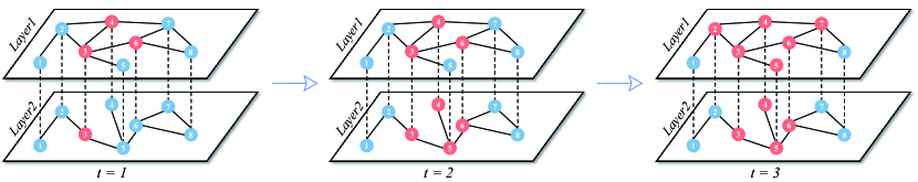
We propose an independent cascade model that is suitable to replicate the dynamics of propagation in a multilayer network (MIC), where propagation occurs simultaneously across different layers. In MIC, we classify nodes into two different categories, that is, active nodes and inactive nodes. Each node can infect its neighbors only once. When a node is infected at one layer of the network and turns to the active state, it will be active across all layers and will become infectious and can infect its neighbors at any layer. The details of MIC are given below.
-
1.
Initially, the seeds are assigned to the active state, and the remaining nodes are in the inactive state.
-
2.
At time step , assuming that the contagion process reaches layer , we first find the active nodes in this layer. For each active node , the inactive neighbors of in layer are denoted as . For each , it will be activated by with independent probability and will be in an active state if activated.
-
3.
At time step , the contagion process will occur in layer and performs similarly to those at time step . It should be noted that if , the propagation at will be in the first layer.
-
4.
The contagion process continues until no new nodes are activated.
We show an example of MIC in a two-layered network in Figure 1. We assign a seed node as . At time step , the inactive neighbors of node at the first layer are given by the set and each will be activated by with probability . As shown in the figure, nodes and are successfully activated. Subsequently, the activated nodes at the beginning of step are , , and , and will activate each of their inactive neighbors with probability in the second layer. As a consequence, node is successfully activated. At step , the propagation will return to layer 1 and the newly activated nodes are and .
2.3 Data description
In this section, we give a summary of four multilayer networks111https://manliodedomenico.com/data.php that exist in the real world, focusing on their fundamental topological characteristics. Detailed descriptions of the datasets are given below:
CKM Physicians Innovation Network (CKM) [32]. CKM dataset illustrates how physicians used the new drug tetracycline in four towns. The interactions of each layer between physicians are constructed according to the following three questions: i) If you need advice about therapy, who do you usually ask? ii) Which three or four physicians do you usually talk to about cases or treatments during a typical week, such as last week? iii) Can you tell me the first names of the three people you spend the most time with socially? The three layers are named shortly as Adv, Dis and Fri, respectively. We construct three two-layered networks using this data: Adv-Dis, Adv-Fri, and Dis-Fri.
London Multiplex Transport Network (Transport) [33]. This dataset was obtained from the official website of the London Transport Authority in 2013. It includes three separate layers: the underground (U), the overground (O), and the Docklands light railway (D) network. The nodes represent the transport stations in London, while the edges represent the existing routes between the stations while using different transportation tools. We construct three two-layer networks based on this dataset, i.e., U-O, U-D, and O-D.
Arxiv Netscience Multiplex (Arxiv) [34]. The Arxiv dataset includes co-authorship between authors in three distinct Arxiv categories: mathematical physics (MP), quantitative biology (QB), and quantitative biomolecules (QBM). In each layer of the network, node represents the authors and the edges represent the co-authorship between the authors. Consequently, we can construct three two-layered networks using this dataset, i.e., MP-QBM, MP-QB, and QBM-QB.
C.elegans Multiplex Gpi Network (C.elegans) [35]. The C.elegans dataset indicates the genetic-protein interaction (GPI) of C.elegans. Each layer of C.elegans represents one type of interaction within the organism, namely physical interactions (Phy), suppressive interactions (SI) or additive interactions (AI). In C.elegans, nodes correspond to proteins, while edges encode protein-protein interaction relationships. Based on this dataset, we construct three two-layered networks: Phy-AG, Phy-SG, and SG-AG.
Using the four multiplexes mentioned above, we can obtain two-layer networks, which are subsequently used to evaluate the performance of the algorithms to solve the IM problem. A comprehensive summary of the basic topological properties of the networks is presented in Table 1.
| Dataset | Two-layer | Layer | |||||
|---|---|---|---|---|---|---|---|
| Adv-Dis | Adv | 234 | 449 | 3.8376 | 0.2600 | 0.0165 | |
| Dis | 234 | 498 | 4.2600 | 0.2598 | 0.0183 | ||
| CKM | Adv-Fri | Adv | 238 | 449 | 3.7731 | 0.2600 | 0.0159 |
| Fri | 238 | 423 | 3.5500 | 0.2108 | 0.0150 | ||
| Dis-Fri | Dis | 241 | 498 | 4.1328 | 0.2598 | 0.0172 | |
| Fri | 241 | 423 | 3.5100 | 0.2108 | 0.0146 | ||
| U-O | U | 330 | 312 | 1.8909 | 0.0311 | 0.0057 | |
| O | 330 | 83 | 0.5000 | 0.0000 | 0.0015 | ||
| Transport | U-D | U | 311 | 312 | 2.0064 | 0.0311 | 0.0065 |
| D | 311 | 46 | 0.3000 | 0.0185 | 0.0010 | ||
| O-D | O | 126 | 83 | 1.3175 | 0.0000 | 0.0105 | |
| D | 126 | 46 | 0.7300 | 0.0185 | 0.0058 | ||
| MP-QBM | MP | 2152 | 592 | 0.5502 | 0.8579 | 0.0003 | |
| QBM | 2152 | 4423 | 4.1100 | 0.7670 | 0.0019 | ||
| Arxiv | MP-QB | MP | 1013 | 592 | 1.1688 | 0.8579 | 0.0012 |
| QB | 1013 | 868 | 1.7100 | 0.6908 | 0.0017 | ||
| QBM-QB | QBM | 2510 | 4423 | 3.5243 | 0.7670 | 0.0014 | |
| QB | 2510 | 868 | 0.6900 | 0.6908 | 0.0003 | ||
| Phy-AI | Phy | 1224 | 270 | 0.4412 | 0.1743 | 0.0004 | |
| AI | 1224 | 2115 | 3.4600 | 0.1338 | 0.0028 | ||
| Celegans | Phy-SI | Phy | 333 | 270 | 1.6216 | 0.1743 | 0.0049 |
| SI | 333 | 160 | 0.9600 | 0.0162 | 0.0029 | ||
| AI-SI | AI | 1121 | 2115 | 3.7734 | 0.1338 | 0.0034 | |
| SI | 1121 | 160 | 0.2900 | 0.0162 | 0.0003 |
3 Algorithms
3.1 Adaptive Coupling Degree
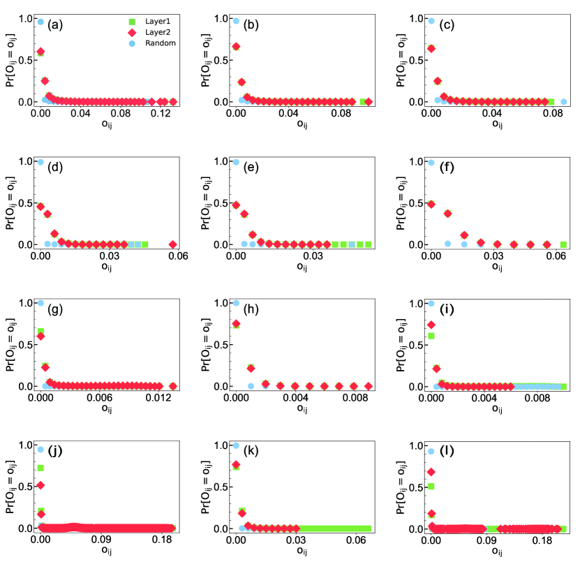
To solve the influence maximization problem, we not only need to choose nodes with a high influence but also need to consider influence overlap between nodes. If a node with high influence is chosen as the seed, the nodes that have a large influence overlap with should have a low chance of being chosen as the seeds, as they cannot help increase the influence margin. We demonstrate the distribution of the influence overlap of nodes in empirical multilayer networks in Figure 2. Particularly, the influence overlap between nodes and is denoted as , where denotes the spreading influence of node when is chosen as the seed. We compare the distribution of the influence overlap of the pairs of neighboring nodes in the first layer, in the second layer, and the pairs of randomly selected nodes. The results show that, compared to the random case, the influence overlap distribution of the neighboring nodes is more oriented to the right, indicating that neighboring nodes have a much larger influence overlap.
Motivated by the above analysis, we propose an adaptive coupling degree (ACD) algorithm for seed node selection in a multilayer network, which aims to find nodes with high spread influence and low influence overlap. To start, we define the coupling degree of a node as the number of non-repetitive neighbors across layers, the formula can be described as:
| (2) |
where represents the neighboring set of in the -th layer. Then we iteratively compute the adaptive coupling degree of each node and choose the nodes with the highest adaptive coupling degree as the seeds. The initialization of the adaptive coupling degree of each node is given by the value of its coupling degree, i.e., . We further define the number of seed nodes in the neighborhood of node as . Therefore, the initial number of seed nodes in the neighborhood of every node is 0, and thus we obtain a vector . Therefore, the procedures to iteratively select the seeds are given below.
-
1.
At the first step, node with the highest adaptive coupling degree () is chosen as the first seed node and added to the seed set . Then, we compute the number of seed nodes in the neighborhood of every node and get . The adaptive coupling degree of node is updated using the following equation:
(3) -
2.
At time step , we order the nodes according to their adaptive coupling degree, which is determined by the vector , and pick the one with the highest degree from and add it to . Similarly, we update the vector based on the number of seed nodes in the neighbors of each node and obtain . Therefore, the adaptive coupling degree of every node is updated based on and :
(4) -
3.
The algorithm terminates when seeds are selected.
In ACD, we use the adaptive coupling degree to quantify a node’s spread influence, the nonlinear penalty factor introduced by is used to filter nodes with low overlap influence, as shown in Eq. 3 and 4. The pseudocode of ACD is provided in Algorithm 1.
3.2 Baselines
To assess the effectiveness of our algorithm, we introduce three state-of-the-art previously proposed methods and extend five centrality-based methods as baselines. We show the details of each of them below.
CBIM [28] is a community-based influence maximization algorithm that considers both node degree and the distance between the nodes. CBIM first conducts community detection in each layer by computing the similarity between nodes. Concretely, the similarity between node and in layer is , where and denote neighboring sets of and , respectively. After obtaining the final communities, we define the edge weight sum (EWS) of each node in each community as , where is the number of paths from node to node of length , denotes the degree of node and is a decay factor (we choose ). The nodes with the largest value of EWS are chosen as the seeds in each layer. To obtain seed nodes, the number of seeds chosen from each community is positively correlated with the size of the community.
KSN [26] is a knapsack seeding algorithm that first uses the CELF++ algorithm [7] to obtain the expected influences of seed nodes of different sizes. The optimal seeds are determined by combining the solutions of each layer such that the sum of the expected influence spread of the selected seed sets is maximized and the size of the union of the selected seed sets is equal to .
CIM [27] is a clique-based heuristic algorithm that identifies seed nodes based on maximal clique222In a network, if a complete graph is not contained in any other complete graph then forms a maximal clique.. CIM finds all maximal cliques in the multilayer network and ranks these cliques in descending order according to their size. Then CIM selects nodes with the highest degree in each maximal clique as seeds. If the number of maximal cliques , the algorithm continues to select nodes with second largest degree from the maximal cliques following the descending order of their size. The selection process continues until the size of the seed node set reaches .
LAD measures the importance of a node by calculating the layered average degree (LAD) for each node, i.e., , is the degree of node in the -th layer, is the number of layers. LAD algorithm selects nodes with the highest LAD values in the network as seed nodes.
CD is a heuristic algorithm based on coupling degree. We calculate the coupling degree of each node and pick the nodes with the highest coupling degrees to be the seed nodes.
Eigenvector considers a node’s importance based on the importance of its neighboring nodes. The eigenvector first calculates the eigenvector centrality values of all nodes in each layer. The final eigenvector of each node is the average of its centrality values of eigenvectors from each layer. We choose the nodes with the highest eigenvector centrality values as seed nodes.
Pagerank first computes the PageRank values of each node in each layer. The final PageRank value of a node is the average of its PageRank values from each layer. The nodes with the highest final PageRank values are chosen as seeds.
Betweenness centrality first computes the betweenness of a node in each layer. The final betweenness value of a node is the average of the betweenness values over all the layers. The seed nodes with the highest Betweenness values are selected as seeds.
The experiments are conducted to compare the effectiveness and robustness of different algorithms. Using the MIC model, we count the number of activated nodes at the end of the spreading process as the spread influence of a set of seed nodes. In our experiments, the size of the seed set ranged from 1 to 50 and the spread influence is the average over 1000 Monte Carlo simulations. All algorithms were implemented in Python and executed independently on a server with a 2.20GHz Intel(R) Xeon(R) Silver 4114 CPU and 90GB of memory.
4 Performance evaluation
4.1 Experimental results on synthetic multilayer networks
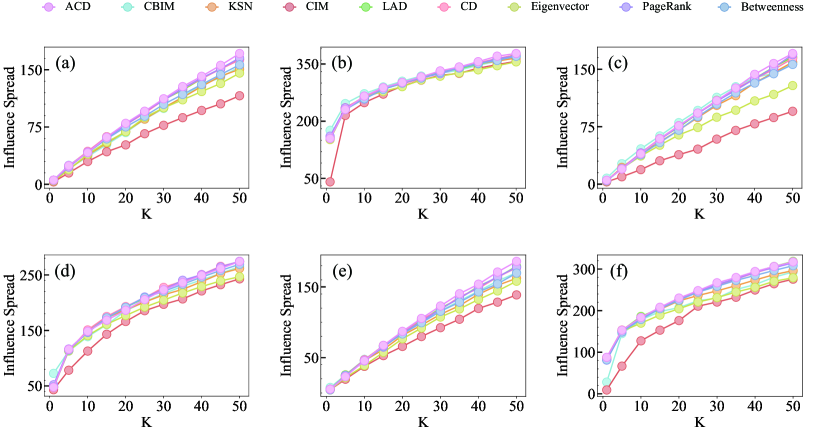
We evaluate the performance of our algorithm on synthetic multilayer networks created using the ER (Erdős-Rényi), BA (Barabási-Albert), and WS (Watts-Strogatz) models, with network size . Specifically, an ER network is generated by starting with an empty network containing nodes and traversing all pairs of nodes , the edge between node and node is added with a probability of . To construct a WS network, the process begins with a cyclic network of 1500 nodes. Each node is connected to its four closest neighbors. Then, each edge is randomly reconnected with a probability of 0.3, introducing randomness into the network. A BA network is established with an initial network that has three nodes and two edges. Whenever a new node is added to the network, it will be connected to two existing nodes through a preferential attachment mechanism. This means that nodes tend to link up with nodes that have a higher degree. Given the three networks obtained above, we combine each two of them to form two-layered networks, namely ER-ER, BA-BA, WS-WS, ER-BA, ER-WS, and BA-WS.
Furthermore, we conduct the MIC spreading model on the synthetic multilayer networks with spreading probability and use influence maximization algorithms to identify seeds. The results in Figure 3 demonstrate that the proposed ACD algorithm surpasses the other algorithms in terms of spreading capacity. On the other hand, the heuristic algorithms that disregard the interconnection between layers perform poorly, sometimes even worse than the centrality-based methods.
4.2 Experimental results on real-world multilayer networks
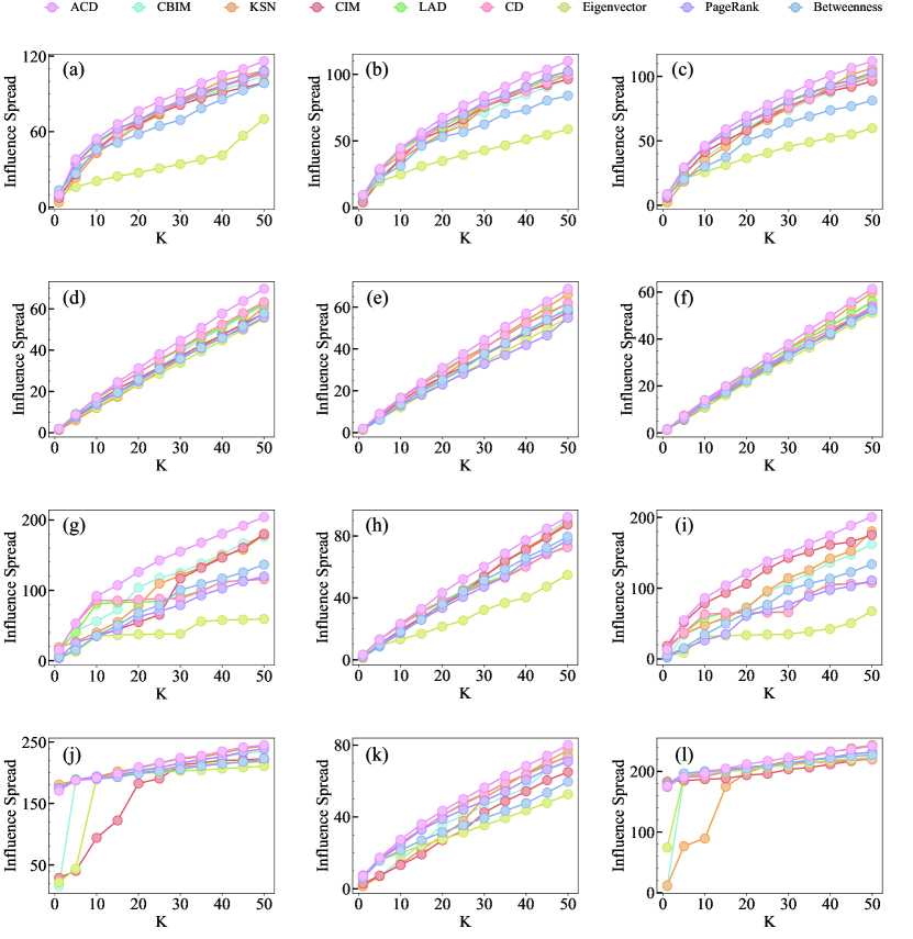
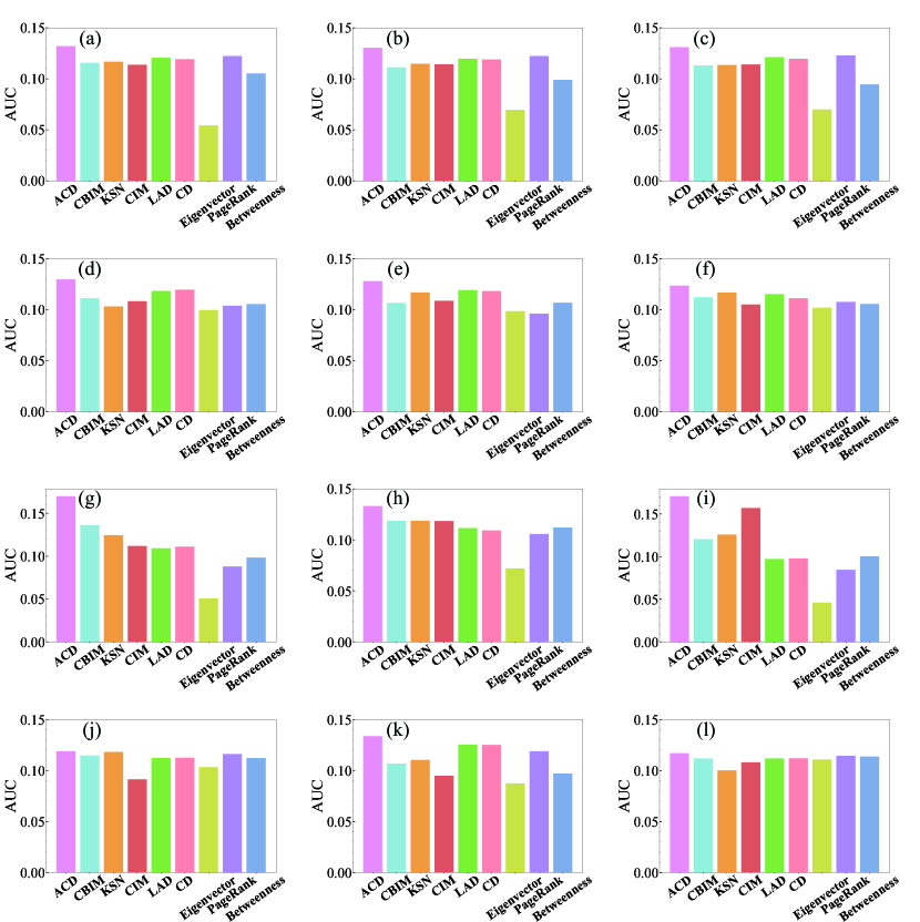
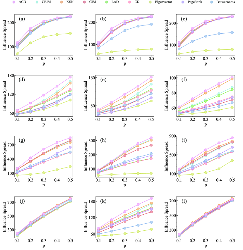
We further evaluate the performance of ACD on multilayer networks generated from four datasets, CKM, Transport, Arxiv, and C.elegans, using the MIC spreading model described in the Section of Preliminary definition. In the MIC model, the contagion probability is set to . We use the final number of infected, i.e., influence spread in the vertical coordinate shown in Figure 4, deduced by the seeds as a metric to evaluate the performance of ACD. The average performance of each algorithm is represented by the area under the influence spread curve, as seen in Figure 5. Combining the two figures, we observe that ACD performs the best across all multilayer networks. Remarkably, ACD, LAD, and CD are all degree-based methods, the gap between ACD and the other two indicates that selecting nodes with low influence overlap can dramatically improve the accuracy of seed node identification. Our algorithm is one of several heuristic approaches to address the influence maximization problem, which is the same as CBIM and CIM. KSN is a greedy algorithm that sacrifices speed for improved performance. Nevertheless, the three algorithms are not as effective as ACD, which could be due to their disregard for the coupling effect between layers when constructing the algorithms. Eigenvector, PageRank, and Betweenness, which are global centrality measures, do not work well on empirical multilayer networks, particularly Eigenvector. This could be due to the presence of isolated nodes in multilayer networks. The eigenvector is not ideal since isolated nodes lack connections from other nodes to affect their eigenvector values, leading to an overestimation of their importance.
The time cost of different algorithms is presented in Table 2 when the seed size is . We remark that the time cost is only for the seed node selection process without considering the MIC contagion process. ACD requires less time to complete than CBIM, KSN, and Betweenness. The difference could be attributed to additional operations, such as community detection and merging in CBIM as well as the greedy strategy in KSN for each layer of the network. Furthermore, for the betweenness centrality, it takes a lot of time to compute the shortest paths between each pair of nodes in the network. ACD is an iterative algorithm that considers both the influence of a node as well as the influence overlap between nodes, resulting in a slightly higher time cost compared to CIM, CD, Degree, Eigenvector, and PageRank. Overall speaking, ACD is more effective than baselines and requires an acceptable amount of time to identify seed nodes for IM in multilayer networks.
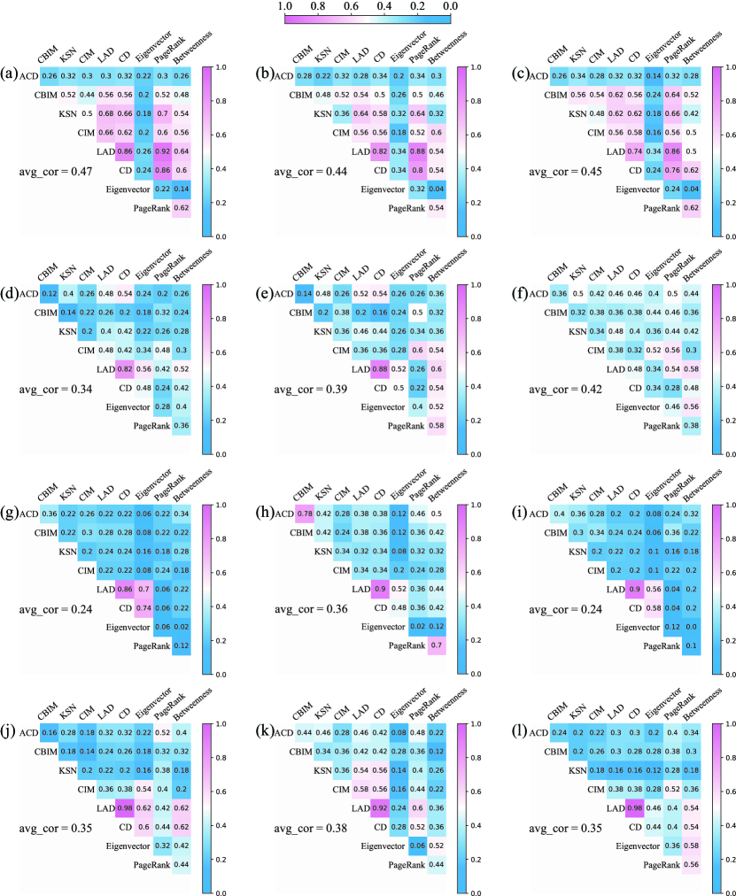
We show the correlation between ACD and the other baselines by computing the seed similarity between them for the seed size . Specifically, for two algorithms and , we suppose that the seed sets obtained by them are and . Therefore, the similarity of the seed sets is defined as . The illustration in Figure 6 displays the similarity between the seeds acquired by distinct algorithms in various multilayer networks. In addition, the average similarity value () is presented, which is the mean of all values in each of the upper triangular matrices. The results show that the seeds obtained by ACD are quite different from the baselines, with most of the similarity values lower than the average values.
| Dataset | multiplex | ACD | CBIM | KSN | CIM | LAD | CD | Eigenvector | PageRank | Betweenness |
|---|---|---|---|---|---|---|---|---|---|---|
| Ad-Dis | 0.0038 | 9.7406 | 33.1708 | 0.0070 | 0.0004 | 0.0021 | 0.3403 | 0.0026 | 0.0414 | |
| CKM | Ad-Fri | 0.0038 | 9.4953 | 30.4458 | 0.0071 | 0.0003 | 0.0023 | 0.3452 | 0.0027 | 0.0405 |
| Dis-Fri | 0.0036 | 10.2109 | 29.6869 | 0.0069 | 0.0003 | 0.0018 | 0.0665 | 0.0030 | 0.0430 | |
| U-O | 0.0050 | 0.3269 | 21.2453 | 0.0044 | 0.0010 | 0.0016 | 0.0153 | 0.0031 | 0.0764 | |
| Transport | U-D | 0.0051 | 0.3036 | 17.8422 | 0.0043 | 0.0010 | 0.0011 | 0.0125 | 0.0030 | 0.0700 |
| O-D | 0.0047 | 0.0382 | 18.1863 | 0.0032 | 0.0012 | 0.0006 | 0.0072 | 0.0028 | 0.0086 | |
| MP-QBM | 0.1971 | 16.4488 | 406.7342 | 0.0334 | 0.0610 | 0.0182 | 0.0725 | 0.0074 | 1.3757 | |
| Arxiv | MP-QB | 0.1859 | 2.4575 | 679.5698 | 0.0110 | 0.0590 | 0.0053 | 0.0396 | 0.0040 | 0.0463 |
| QBM-QB | 0.2004 | 17.4843 | 1699.3893 | 0.0295 | 0.0564 | 0.0189 | 0.0794 | 0.0080 | 1.3807 | |
| Phy-AI | 0.0523 | 563.6921 | 1345.1427 | 0.0172 | 0.0154 | 0.0073 | 0.0358 | 0.0173 | 1.4071 | |
| Celegans | Phy-SI | 0.0508 | 1.1359 | 266.7521 | 0.0053 | 0.0159 | 0.0013 | 0.0089 | 0.0041 | 0.0162 |
| SI-AI | 0.0516 | 547.2645 | 1283.2126 | 0.0133 | 0.0155 | 0.0062 | 0.0325 | 0.0060 | 1.3649 |
Robustness analysis
The robustness of ACD is evaluated by changing the contagion probability of MIC when the seed size is , as shown in Figure 7. We present the results of ranging from to with an interval of , as a value of that is too high could cause the propagation process to cover most nodes in the network regardless of the selected seeds. As increases, the spread of influence also increases, yet ACD usually performs best across different networks. Figure 7 j and l demonstrate two exceptions, where KSN has the highest performance when the spread probability is greater than , while ACD is still the second best. The results demonstrate the efficacy of the ACD algorithm in a variety of spread probabilities, particularly in terms of its superior performance in most cases.
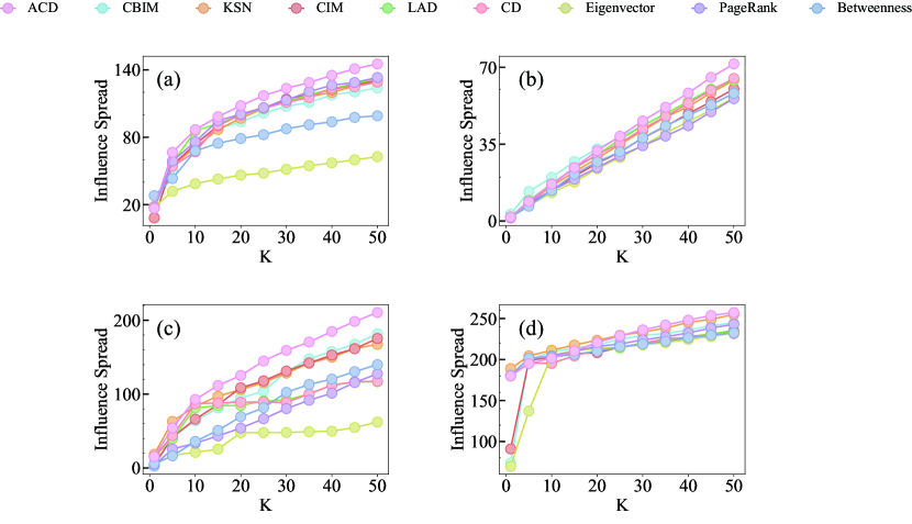
We further test the effectiveness of ACD in three-layer networks when the contagion probability . As shown in Figure 8, ACD performs almost optimally in all four three-layer networks, with some exceptions when is small. We observe that ACD performs better when is larger. The good performance of ACD in two- and three-layer empirical networks indicates its robustness across multilayer networks from different areas.
Conclusion
The main challenge of solving the IM problem on a multilayer network is how to combine topological information of one node upon different layers, especially incorporating the coupling effect between layers. In this work, we propose a method named Adaptive Coupling Degree (ACD), which iteratively selects seed nodes with low influence overlap between each other and a high coupling degree. Additionally, a spreading model, i.e., MIC, which considers a piece of information spreading through a multilayer network and enhances inter-layer spread interactions, is proposed to quantify the spread influence of the nodes selected by our method.
To validate the effectiveness of our algorithm, we conduct extensive experiments on four empirical multilayer networks, which are generated by complex systems from different scenarios, such as social networks, transportation networks, and biological networks. We compare the performance of ACD with eight baseline algorithms, and the experimental results demonstrate that ACD exhibits a significantly wider influence spread than the baseline algorithms. Moreover, we assess the robustness of ACD across various empirical and synthetical multilayer networks, highlighting its effectiveness in diverse network structures.
The limitation of our work is that we only consider the fundamental topological structure to design the algorithm for the IM problem. However, researchers have claimed that the dynamic process may also affect the effectiveness of the algorithms [36, 37]. In future work, the dynamic aspect of the nodes should also be considered and a general framework that can be adapted to different spreading models, such as as multilayer linear threshold models [38], multilayer susceptible-infected-susceptible (SIS) models [39], and other propagation mechanisms [40], should be designed. Additionally, more effort should be made to solve the extensive IM problems on multilayer networks, i.e., budgeted IM [12, 13], competitive IM [14, 15], and targeted IM [16, 17, 18].
5 Declaration of competing interest
The authors declare that they have no known competing financial interests or personal relationships that could have appeared to influence the work reported in this paper.
6 Data availability
Data will be available on request.
7 Acknowledgement
This work was supported by the Natural Science Foundation of Zhejiang Province (Grant No. LQ22F030008), the Natural Science Foundation of China (Grant No. 61873080) and the Scientific Research Foundation for Scholars of HZNU (2021QDL030).
References
- [1] Kempe D, Kleinberg J, Tardos É. Maximizing the spread of influence through a social network. In Proceedings of the ninth ACM SIGKDD international conference on Knowledge discovery and data mining. Association for Computing Machinery, pages 137–146. https://doi.org/10.1145/956750.956769.
- [2] Chen W, Wang C, Wang Y. Scalable influence maximization for prevalent viral marketing in large-scale social networks. In Proceedings of the 16th ACM SIGKDD international conference on Knowledge discovery and data mining. Association for Computing Machinery, pages 1029–1038. https://doi.org/10.1145/1835804.1835934.
- [3] Domingos P, Richardson M. Mining the network value of customers. In Proceedings of the seventh ACM SIGKDD international conference on Knowledge discovery and data mining. Association for Computing Machinery, pages 57–66. https://doi.org/10.1145/502512.502525.
- [4] Cheng C, Kuo Y, Zhou Z. Outbreak minimization vs influence maximization: an optimization framework. BMC Medical Inform Decis Mak 2020;20(1):1–13. https://doi.org/10.1186/s12911-020-01281-0.
- [5] Zhang H, Mishra S, Thai MT, Wu J, Wang Y. Recent advances in information diffusion and influence maximization in complex social networks. Opportunistic Mobile Social Networks 2014;37(1.1):37–70. https://books.google.co.jp/books?id=o3nSBQAAQBAJ.
- [6] Leskovec J, Krause A, Guestrin C, Faloutsos C, VanBriesen J, Glance N. Cost-effective outbreak detection in networks. In Proceedings of the 13th ACM SIGKDD international conference on Knowledge discovery and data mining. pages 420–429. https://doi.org/10.1145/1281192.1281239.
- [7] Goyal A, Lu W, Lakshmanan LV. Celf++ optimizing the greedy algorithm for influence maximization in social networks. In Proceedings of the 20th international conference companion on World wide web. pages 47–48. https://doi.org/10.1145/1963192.1963217 .
- [8] Xie M, Zhan X, Liu C, Zhang Z. An efficient adaptive degree-based heuristic algorithm for influence maximization in hypergraphs. Inf Process Manag 2023;60(2):103161. https://doi.org/10.1016/j.ipm.2022.103161.
- [9] Xie X, Zhan X, Zhang Z, Liu C. Vital node identification in hypergraphs via gravity model. Chaos 2023;33(1):013104. https://doi.org/10.1063/5.0127434.
- [10] Yang P, Zhao L, Lu Z, Zhou L, Meng F, Qian Y. A new community-based algorithm based on a “peak-slope-valley” structure for influence maximization on social networks. Chaos Solitons Fractals 2023;173:113720. https://doi.org/10.1016/j.chaos.2023.113720.
- [11] Li Q, Cheng L, Wang W, Li X, Li S, Zhu P. Influence maximization through exploring structural information. Appl Math Comput 2023;442:127721. https://doi.org/10.1016/j.amc.2022.127721.
- [12] Nguyen H, Zheng R. On budgeted influence maximization in social networks. IEEE J Sel Areas Commun 2013;31(6):1084–1094. https://doi.org/10.1109/JSAC.2013.130610.
- [13] Banerjee S, Jenamani M, Pratihar DK. ComBIM: A community-based solution approach for the Budgeted Influence Maximization Problem. Expert Syst Appl 2019;125:1–13. https://doi.org/10.1016/j.eswa.2019.01.070.
- [14] Bharathi S, Kempe D, Salek M. Competitive influence maximization in social networks. In Internet and Network Economics: Third International Workshop. Springer, pages 306–311. https://doi.org/10.1007/978-3-540-77105-0_31.
- [15] Bozorgi A, Samet S, Kwisthout J, Wareham T. Community-based influence maximization in social networks under a competitive linear threshold model. Knowl Based Syst 2017;134:149–158. https://doi.org/10.1016/j.knosys.2017.07.029.
- [16] Cai T, Li J, Mian A, Li R, Sellis T, Yu J. Target-aware holistic influence maximization in spatial social networks. IEEE Trans Knowl Data Eng 2020;34(4):1993–2007. https://doi.org/10.1109/TKDE.2020.3003047.
- [17] Caliò A, Tagarelli A. Attribute based diversification of seeds for targeted influence maximization. Inf Sci 2021;546:1273–1305. https://doi.org/10.1016/j.ins.2020.08.093.
- [18] Liang Z, He Q, Du H, Xu W. Targeted influence maximization in competitive social networks. Inf Sci 2023;619:390–405. https://doi.org/10.1016/j.ins.2022.11.041.
- [19] Kivelä M, Arenas A, Barthelemy M, Gleeson JP, Moreno Y, Porter MA. Multilayer networks. J Complex Netw 2014;2(3):203–271. https://doi.org/10.1093/comnet/cnu016J.
- [20] Watts DJ, Strogatz SH. Collective dynamics of ‘small-world’networks. Nature 1998;393(6684):440–442. https://doi.org/10.1038/30918.
- [21] Buccafurri F, Lax G, Nicolazzo S, Nocera A. A model to support multi-social-network applications. In On the Move to Meaningful Internet Systems: OTM 2014 Conferences. Springer, pages 639–656. https://doi.org/10.1007/978-3-662-45563-0_39.
- [22] Al-Garadi MA, Varathan KD, Ravana SD, Ahmed E, Chang V. Identifying the influential spreaders in multilayer interactions of online social networks. J Intell Fuzzy Syst 2016;31(5):2721–2735. https://doi.org/10.3233/JIFS-169112.
- [23] Kuzmanov U, Emili A. Protein-protein interaction networks: probing disease mechanisms using model systems. GENOME MED 2013;5(4):1–12. https://doi.org/10.1186/gm441.
- [24] Kenley EC, Cho YR. Detecting protein complexes and functional modules from protein interaction networks: A graph entropy approach. Proteomics 2011;11(19):3835–3844. https://doi.org/10.1002/pmic.201100193.
- [25] Gallotti R, Barthelemy M. The multilayer temporal network of public transport in Great Britain. Sci Data 2015;2(1):1–8. https://doi.org/10.1038/sdata.2014.56.
- [26] Kuhnle A, Alim MA, Li X, Zhang H, Thai MT. Multiplex influence maximization in online social networks with heterogeneous diffusion models. IEEE Trans Comput Soc Syst 2018;5(2):418–429. https://doi.org/10.1109/TCSS.2018.2813262.
- [27] Katukuri M, Jagarapu M. CIM: clique-based heuristic for finding influential nodes in multilayer networks. Appl Intell 2022;52(5):5173–5184. https://doi.org/10.1007/s10489-021-02656-0.
- [28] Rao KV, Chowdary CR. CBIM: Community-based influence maximization in multilayer networks. Inf Sci 2022;609:578–594. https://doi.org/10.1016/j.ins.2022.07.103.
- [29] Hu X, Zhao Y, Yang Z. Nodes Grouping Genetic Algorithm for Influence Maximization in Multiplex Social Networks. In 2023 26th International Conference on Computer Supported Cooperative Work in Design (CSCWD). IEEE, pages 1130–1135. https://doi.org/10.1109/CSCWD57460.2023.10152626.
- [30] Wang S, Liu J, Jin Y. Finding influential nodes in multiplex networks using a memetic algorithm. IEEE Trans Cybern 2019;51(2):900–912. https://doi.org/10.1109/TCYB.2019.2917059.
- [31] Li S, Li X. Influence maximization in hypergraphs: A self-optimizing algorithm based on electrostatic field. Chaos Solitons Fractals 2023;174:113888. https://doi.org/10.1016/j.chaos.2023.113888.
- [32] Coleman J, Katz E, Menzel H. The diffusion of an innovation among physicians. Sociometry 1957;20(4):253–270. https://doi.org/10.2307/2785979.
- [33] De Domenico M, Solé-Ribalta A, Gómez S, Arenas A. Navigability of interconnected networks under random failures. P NATL A SCI 2014;111(23):8351–8356. https://doi.org/10.1073/pnas.1318469111.
- [34] De Domenico M, Lancichinetti A, Arenas A, Rosvall M. Identifying modular flows on multilayer networks reveals highly overlapping organization in interconnected systems. Phys Rev X 2015;5(1):2160–2170. https://doi.org/10.1103/PhysRevX.5.011027.
- [35] De Domenico M, Nicosia V, Arenas A, Latora V. Structural reducibility of multilayer networks. Nat Commun 2015;6(1):6864. https://doi.org/10.1038/ncomms7864.
- [36] Gong M, Yan J, Shen B, Ma L, Cai Q. Influence maximization in social networks based on discrete particle swarm optimization. Inf Sci 2016;367:600–614. https://doi.org/10.1016/j.ins.2016.07.012.
- [37] Lu W, Zhou C, Wu J. Big social network influence maximization via recursively estimating influence spread. Knowl Based Syst 2016;113:143–154. https://doi.org/10.1016/j.knosys.2016.09.020.
- [38] Zhong Y, Srivastava V, Leonard NE. Influence spread in the heterogeneous multiplex linear threshold model. IEEE Trans Control Netw Syst 2021;9(3):1080–1091. https://doi.org/10.1109/TCNS.2021.3088782.
- [39] Paré PE, Janson A, Gracy S, Liu J, Sandberg H, Johansson KH. Multilayer SIS Model With an Infrastructure Network. IEEE Trans Control Netw Syst 2022;10(1):295–307. https://doi.org/10.1109/TCNS.2022.3203352.
- [40] Bródka P, Musial K, Jankowski J. Interacting Spreading Processes in Multilayer Networks: A Systematic Review. IEEE Access 2020;8:10316–10341. https://doi.org/10.1109/ACCESS.2020.2965547.