Influence of initial states on memory effects: A study of early-time superradiance
Abstract
The initial states of a quantum system can significantly influence its future dynamics, especially in non-Markovian quantum processes due to the environmental memory effects. Based on a previous work of ours, we propose a method to quantify the memory effects of a non-Markovian quantum process conditioned on a particular system initial state. With this method, we analytically study the early-time memory effects of a superradiance model consisting of atoms (the system) interacting with a single-mode vacuum cavity (the environment) with two types of initial states: the Dicke states and the factorized identical states. We find that the radiation intensity are closely related to the memory effects, and correspondingly, the enhancement of memory effects (from independent radiation to collective radiation) is important for the degree of superradiance, especially for the Dicke states. Furthermore, numerical results in other regimes show that the characteristics of memory effects and superradiance in longer-time dynamics can be reflected through its early-time dynamics.
I Introduction
The initial state of a quantum system can significantly influence its future dynamics [1, 2], especially in non-Markovian quantum processes due to the environmental memory effects. One trivial example is that if the system is initially in a steady state in a non-Markovian quantum process, it can hardly exhibit any non-Markovian features afterward, such as the nonmonotonic behaviors of energy and information flows [3, 4, 5, 6]. More intriguing phenomena may emerge when a system consists of a collection of subsystems, such that the properties of its initial state, such as entanglement and coherence, may significantly influence its future dynamics. A well-known example is the concept of superradiance [7, 9, 8, 10, 11, 12, 13, 14] introduced by Dicke in 1954, where the emission intensity from an ensemble of atoms interacting with a common electromagnetic field can be enhanced compared with that from independent atoms. It is also well-known that the superradiance behaviors are highly relevant to the initial states of the system. In recent years, superradiance has received a large amount of attention due to its theoretical significance and potential applications [16, 15, 17, 18, 19, 20, 21, 22, 23, 24, 25, 26, 27, 28, 29, 30, 31]. Under certain approximations, such as a coarse-grained timescale, the superradiance process could be regarded as Markovian [10, 11, 12, 13, 14], whereas, it is intrinsically non-Markovian. With the advances in theories and technologies, understanding the non-Markovian dynamics of superradiance becomes more demanding [28, 29, 30, 31]. In a recent work [31], the author shows that non-Markovian memory effects play an important role in superradiance beyond retardation, featuring the quadratic dynamics in the early-time (Zeno) regime, whereas, the memory effects are not quantitatively evaluated. In view of the significant influences of the system initial states on non-Markovian quantum processes, especially, a superradiance process, some interesting questions arise. For example, how to quantitatively evaluate the memory effects of a quantum process conditioned on a particular system initial state? Are there quantitative relations between the memory effects and the superradiance characteristics in the early-time regime? What is the role of the (very weak) memory effects in a superradiance process that could be well approximated as Markovian?
In recent years, a number of measures or manifestations of non-Markovianity were proposed to characterize the memory effects which are often connected to nonmonotonic behaviors [3, 4, 5, 6]. For example, the well-known BLP measure [32] and the RHP measure [33] use the increases of distinguishability and entanglement, respectively, to measure the non-Markovianity. The nonmonotonic behaviors originate from the noncomplete positivity of the intermediate dynamical maps in non-Markovian processes. These measures generally apply to quantum processes where the evolutions start at a fixed time (usually for simplicity). However, a key distinction of the non-Markovian process is the existence of in the generator of the system’s time-local equation, i.e., [34]. Thus some features of non-Markovianity might not be characterized with only evolutions starting from a fixed time . For example, in the early-time regime or a near-Markovian regime, the spontaneous radiation of an atom could be described by a time-local equation with a positive (time-dependent) damping rate, which looks like a time-dependent Markovian master equation (except in its generator) [35]. Thus the nonmonotonic behaviors do not occur in these regimes, implying weaker memory effects. Meanwhile, the non-Markovianity measures based on the noncomplete positivity may give zero memory effects. On the other hand, the previously proposed non-Markovianity measures generally do not depends on a particular system initial state, but deal with a quantum process where all the potential initial states are considered. Therefore, an initial-state-dependent measure which is able to characterize weak memory effects is demanding.
In this paper, we propose such a method developed from a previous work [35] of ours. The non-Markovianity measure in Ref. [35] is based on the inequality of completely positive dynamical maps and connected with the validity of the Markov approximation. By acting the inequality on a particular initial state , the evolutions starting at and have the same system states at but different histories before . Thus the memory effects (past-future dependence) could be understood by the difference between the final states and . Based on the above interpretation, we suggest measuring the memory effects conditioned on the initial state by the maximal difference of and in a time interval of interest. Using this method, we calculate the memory effects (as well as the radiation characteristics) of a superradiance model with two types of initial states: the Dicke states and factorized identical states in different regimes. The model describes two-level atoms interacting with a single-mode cavity initially in vacuum. We give analytic expressions of the characteristics of memory effects (and superradiance) in the early-time regime. Moreover, we extend our work to longer time intervals in the near-Markovian regime, and to the whole radiation lifetime in a strongly non-Markovian regime with numerical results.
The main findings are as follows. 1. The radiation intensity is closely related to the memory effects, and correspondingly, the degree of superradiance is closely related to the degree of memory-effect-enhancement (from independent radiation to collective radiation), especially for the Dicke states. 2. The entanglement in the Dicke states and the single-atom coherence in the factorized identical states are necessary for the superradiance and important for the memory-effect-enhancement. 3. The (change of) environmental photon number is a main physical source of memory effects for our model. 4. The characteristics of memory effects and superradiance in long-time dynamics (especially for the near-Markovian regime) can be reflected through its early-time dynamics.
The paper is organized as follows: In Sec. II, we propose our method to evaluate the initial-state-dependent memory effects in a quantum process. In Sec. III, we obtain the early-time solution of two-level atoms interacting with a vacuum cavity, with which we give analytic expressions for the value of memory effects, the cavity photon number, the degree of superradiance, and so on. In Sec. IV, the influences of two types of initial states on the memory effects as well as the superradiance are calculated and analyzed using the early-time results. Our work is extended to the near-Markovian regime and a strongly non-Markovian regime in Sec. V. At last, conclusions and discussions are presented in Sec. VI.
II Initial-state-dependent memory effects
In this section, we first review the measure of non-Markovianity in Ref. [35], which quantifies the memory effects (the past-future dependence) in a quantum process. Using its physical interpretations, we then propose a method to quantify the memory effects in a quantum process conditioned on a particular initial state of the system. The object of study in Ref. [35] is a quantum process of an open quantum system described by the total Hamiltonian
| (1) |
an arbitrary system initial state and a fixed initial state of the environment (independent of the system). Here is the initial time of an evolution which is also arbitrary. The initial condition of an evolution is
| (2) |
which means that the system is initially uncorrelated with the environment before the evolution. In general, is governed by [6]
| (3) |
Typically, one deals with a time-independent environment Hamiltonian and assumes a steady state of as the environmental initial state (e.g., a thermal state). Then, the initial condition of an evolution is
| (4) |
for any . Since and is arbitrary, the measure of non-Markovianity (memory effects) in Ref. [35] is determined by and and the time interval of interest.
In a non-Markovian quantum process, the meaning of a dynamical map given by is ambiguous unless , or from another perspective, the initial time is specified (). For clarity, we define as a memoryless dynamical map that transfers to , where is the initial time of the evolution () [35], i.e.,
| (5) | |||||
where is fixed, is arbitrary and in general. Particularly, when is time-independent and is a steady state of , Eq. (5) is simplified to
| (6) | |||||
such that [34]. The dynamical map is trace-preserving and completely positive and called a universal dynamical map (UDM) that is independent of the state it acts upon [36].
Let , a (time-dependent) quantum process is Markovian if the dynamical maps (denoted by ) satisfy the divisibility condition
| (7) |
where each dynamical map is uniquely defined and a UDM. Remark that the dynamical map is a UDM if and only if it is induced by
| (8) | |||||
where is fixed and is arbitrary [36]. In an open quantum system, the condition [ does not dependent on the system state] may not be satisfied exactly for . Thus the dynamics of an exact open quantum system is typically not Markovian [36]. However, can be a good approximation where the correlation between the system and the environment does not affect the system’s dynamics so much [36]. It is observed that the Markovian dynamical map is unique and does not depend on the initial time of an evolution, e.g., or . Therefore, according to the definition of the memoryless dynamical map . Then, the Markovian divisibility condition (7) can also be expressed in terms of the memoryless dynamical map by
| (9) |
whose violation is a sign of non-Markovianity. Unlike the dynamical maps used in some non-Markovianity measures [33, 37], all the dynamical maps are completely positive. The violation of Eq. (9) is manifested by the inequality
| (10) |
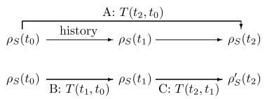
The physical meaning of Eq. (10) can be explained with Fig. 1. Let the left-hand and the right-hand sides of Eq. (10) act on a system initial state . On the left-hand side of Eq. (10), is mapped to by in evolution A. On the right-hand side, is first mapped to by in evolution B. Then, as the initial state of evolution C, is mapped to by , which means that the initial condition of evolution C is with fixed defined by Eq. (3) or a steady one . At moment , evolution A and C have the same system state but different histories: evolution A has a history in time interval , which is encoded in , while evolution C (starting at ) has no history before . Therefore, is an evidence that the future state (after ) of the system depends on its history (in ) in this quantum process. This is the physical meaning of the memory effects in this paper and [35]. Otherwise, if the divisibility (9) holds, the process is Markovian and for any .
On the other hand, the inequality could be understood by focusing on the change of the environment state between evolution B and C. At the end of evolution B, . Then, at the beginning of evolution C, the environment is initialized by such that , where is independent of the system. The information of the system’s history in is erased by . In contrast, such an initialization never happens in evolution A. Therefore, signifies that the environment (as well as the correlations between the system and environment [36]) remembers the system’s history and this memory can influence the future of the system.
In Ref. [35], we define the maximal difference of and as the non-Markovianity where and are optimized. Based on the dynamical maps , all the initial states are potentially considered, thus the measure of non-Markovianity in Ref. [35] does not depend on the initial state of the system. In this paper, our goal is to evaluate the influence of the system initial state on the memory effects in a quantum process. Using the physical interpretations discussed above, we define the value of memory effects conditioned on as the maximal trace distance between and :
| (11) |
Here is the trace norm of an operator . Assuming a fixed for convenience, could be calculated by optimizing and in a time interval of interest where . For example, the time interval might be or , where is finite (as done later in this paper). Similar to the measure in Ref. [35], is satisfied due to the properties of the trace distance.
Using Eq. (11), the influence of initial states on the memory effects of a quantum process could be quantitatively evaluated. Note that is a sufficient condition for the inequality Eq. (10), but not a necessary one. The theoretical calculation and experimental observation of Eq. (11) might be easier than those in Ref. [35] since the determination of the dynamical maps is not compulsory. Moreover, as discussed in Ref. [35], is a sufficient condition for , where is an operator of a physical quantity. Therefore, when the full information of the system state is not easily obtainable, () could be used as an evidence (manifestation) of the memory effects for simplicity and intuitiveness both theoretically and experimentally.
III Early-time superradiance
III.1 Theoretical model
We consider a fundamental model that describes two-level atoms (the system, denoted by “”) interacting with a cavity (the environment, denoted by “” ) initially in a vacuum state. The Hamiltonian is given by
| (12) | |||||
Here and represent noninteracting two-level atoms and a single-mode electromagnetic field in the cavity, respectively. describes the interactions between the atoms and the cavity with the rotating wave approximation, and the coupling strength is a real constant. The lowering and raising operators for the th atom is defined as and .
The initial condition of the model is assumed to be where is arbitrary and is the vacuum state of the cavity. For simplicity, we use in the remainder of this paper without loss of generality. The density matrix of the composite system is described by the master equation,
| (13) | |||||
where is the dissipation strength of the cavity. Assume the cavity is in resonance with the atoms (), then the density matrix in the interaction picture is described by
| (14) | |||||
The superradiance phenomenon could be understood as the enhancement of collective spontaneous radiation caused by a common environment (compared with independent environments). To understand the role of memory effects in the superradiance process, we are also interested in the dynamics where the atoms radiate independently, e.g., each atom radiates in its own cavity. This dynamics could be described by the Hamiltonians , and the environment initial state . Under the resonance condition, the master equation for the independently radiating atoms and the cavities in the interaction picture is given by
| (15) | |||||
III.2 Early-time solution
In this section, we focus on the early-time dynamics where due to the following reasons: First, non-Markovian characters are non-negligible on such a short timescale. Second, it stresses the influence of a particular initial state since the state hardly changes in this time interval. Furthermore, it is helpful for understanding the creation mechanism of the superradiance. In the early-time limit , one might ignore the influence of cavity dissipation , providing that is not infinitely large. In this case, evolves unitarily via
| (16) |
where and . The influence of ignoring on the early-time dynamics will be discussed at the end of this section.
The reduced dynamics of the atoms could be determined by tracing out the degrees of the environment:
| (17) | |||||
where are a set of basis in . With the help of the Baker-Campbell-Hausdorff formula
| (18) |
after the replacement , , and , we have
| (19) | |||||
where the terms with higher orders of have been omitted due to the early-time limit (). Using the number state basis of the cavity and the assumption , it is straightforward to derive the solution of the system evolution in the early-time limit ,
| (20) |
Here is the collective lowering operator and is the Lindblad superoperator. and have been used to obtain Eq. (20). Notice that the partial trace over the second term of Eq. (19) is zero, thus the change of is quadratic in in the early-time limit. Using similar procedures done above, we obtain the early-time solution for independently radiating atoms:
| (21) |
III.3 Memory effects
With the above results, we now calculate the initial-state-dependent memory effects defined in Sec.II. We consider the dynamics in a short time interval where . In “evolution A” (with a history from to ) as mentioned before, the initial state is and the final state is given by
| (22) |
Here and are used for convenience. The initial state of “evolution C” at is
| (23) |
In “evolution C” (without any history before ), the final state is given by
| (24) |
Substituting Eq. (23) into Eq. (24), we have
| (25) | |||||
where the high-order term has been omitted due to the early-time limit. The memory effects are manifested by the difference between Eq. (22) and Eq. (25):
| (26) | |||||
According to Eq. (11), the value of the memory effects for the initial state is
| (27) | |||||
Since is a constant for a given , Eq. (27) can be calculated simply by maximizing with the constraint . Let , then . Therefore, the maximum of is when . It is easy to see that the maximum of in the time interval happens when . Eventually, in the early-time limit is
| (28) | |||||
Equation (28) demonstrates that in a short time interval , grows quadratically with . To focus on the influence of initial states (rather than the time or the atom-cavity coupling ), it is convenient to discuss the normalized value of memory effects
| (29) |
It represents the strength of memory effects in the early-time limit as a function of only . Notice that is not bounded as . In principle, there is . Similarly, the normalized memory effects for independent cavities (denoted by ) can be derived from Eq. (21). The result can be expressed simply by replacing in Eq. (29) by , i.e.,
| (30) |
III.4 Cavity photon number
In a non-Markovian proceess, the relation does not hold in general. Particularly, for the superradiance problem, the change of photon number in the environment (the cavity) might be an important source of the memory effects so that . Thus it is desirable to know the cavity photon number (denoted by in this paper) in the early-time limit in order to understand the physics of the memory effects. The total excitation number of our model represented by is conserved since . Besides, there are no photon in the cavity initially. Therefore, the cavity photon number is equal to the loss of excitations of the atoms that represents the emission intensity of superradiance (in the early-time limit).
According to Eq. (20), the cavity photon number at for is given by,
| (31) | |||||
Using and , Eq. (31) can be simplified to a more concise form
| (32) |
It is observed that in the early-time limit, the cavity number increases quadratically with time. As mentioned in the last section, it is convenient to discuss the normalized cavity photon number
| (33) |
such that it does not depend on the evolution time and atom-cavity coupling . Equation (33) represents the emission intensity in the early-time limit as a function of only the initial state. When each atom radiates independently, e.g., each atom radiates in its own cavity, the normalized cavity photon number for the th atom is reduced to
| (34) |
where is the reduced density matrix of the th atom. Then the degree of superradiant in the early-time regime might be measured by the ratio [9, 15]
| (35) | |||||
for nonzero denominator. If is greater (less) than one, the state is superradiant (subradiant).
III.5 Other manifestations of memory effects
As discussed in Sec. II, the difference between and can be used as an evidence or a manifestation of the memory effects. For the superradiance problem, the atom excitation number operator serves as a nature choice. Following similar treatments in Eqs. (26)-(28), it is seen that the maximum of the atom excitation difference in the time interval also happens at and
| (36) | |||||
Using the results given by Eq. (31) and (32), the manifestation can be further simplified by
| (37) | |||||
It is seen that the maximal difference of the atom excitation numbers in is exactly half the cavity photon number at in the early-time limit. Therefore, the nonzero cavity photon number itself is also a manifestation of memory effects.
III.6 Early-time regime
Mathematically, Eq. (20) holds true as . One may wonder the validity of the early-time solution Eq. (20) in a longer time interval and how the cavity dissipation deteriorates the validity. In this section, we discuss this problem by comparing the systems dynamics by Eq. (20) with that by numerically solving the full dynamics in with Eq. (14) and tracing out the environment. A dynamics could be represented by the dynamical maps that turns all the possible initial states at to their final states at . Furthermore, the difference of two dynamical maps can be evaluated through their Choi-Jamiółkowski matrices [38, 39]. Here we evaluate the error of Eq. (20) at instant by the trace distance of and , i.e.,
| (38) |
where and are the Choi-Jamiółkowski matrices calculated by Eq. (20) and (14), respectively. The Choi-Jamiółkowski matrix is defined as with a maximally entangled state of the -atom system and an ancillary system of the same dimension.
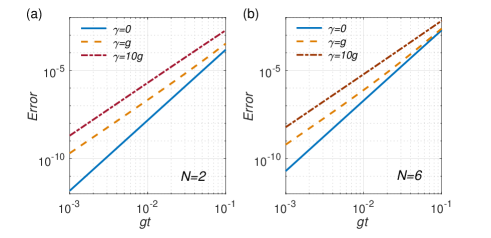
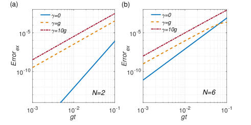
We numerically calculated the error of Eq. (20) for and . The results are illustrated in Fig. 2 in logarithmic scale. It is seen that the order of magnitude of error decreases linearly with that of . Although the cavity dissipation and the increasing of atom number can increase the error, there exists a time interval where Eq. (20) is a good approximation as long as and are finite. For example, in a time interval , the error is less than even when for both and , implying that Eq. (20) is a good approximation in this scenario. The above discussion implies that the early-time limit could be relaxed to an early-time regime, i.e., a time interval where the decay is quadratic. Here is linked to the Zeno time [40, 41, 42, 43]. We also illustrate the difference of the atom excitation numbers from Eqs. (20) and (14), i.e., , in Fig. 3 as another manifestation of the error. The initial states in Figs. 3(a) and 3(b) are 2 and 6 fully excited atoms, respectively. The result is similar to that in Fig. 2 but easier to be verified experimentally.
IV Influence of initial states
In this section, the results Eqs. (29), (30), (33) and (35) are applied to several types of -atom initial states. Our first aim is to study the influence of initial states on the memory effects. Another aim is to reveal the role of memory effect in creating superradiance. Conversely, it also helps to understand the physical source of memory effects in our model.
IV.1 Dicke states
The Dicke states, written as , are extensively studied in the field of superradiance. It is defined as the common eigenstate of the pseudospin operators and with . The eigenvalues are given by
| (39) | |||||
| (40) |
where the operators are defined by , , and . A Dicke state is symmetrical and invariant by atom permutation with excited atoms and ground-state atoms. It can be constructed by the following formula [10]:
| (41) |
For example, for 3 two-level atoms, there is .
A well-known result of the free-space spontaneous emission rate for two-level atoms is , where is the natural linewidth of a single atom. For the Dicke states, there is
| (42) | |||||
When (fully excited), . Then the emission rate is proportional to , or say, the -atom emission rate is equal to the summation of those from independent atoms. Thus there is no superradiance. When (half excited), , the emission rate increase with , or say, the -atom emission rate is greater than the summation of those from independent atoms (). The superradiance with the most intensive emission happens in this case. Note that the results holds under the Born-Markov approximation and on a coarse-grained timescale [10, 11, 12, 13, 14].
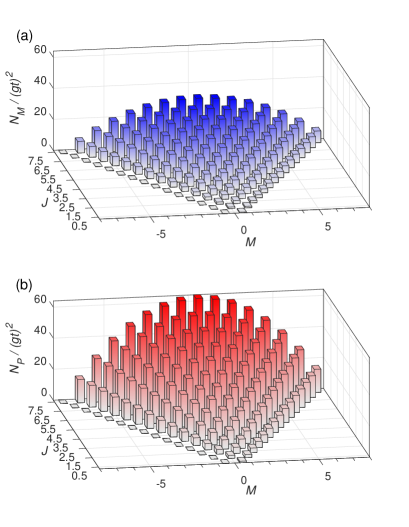
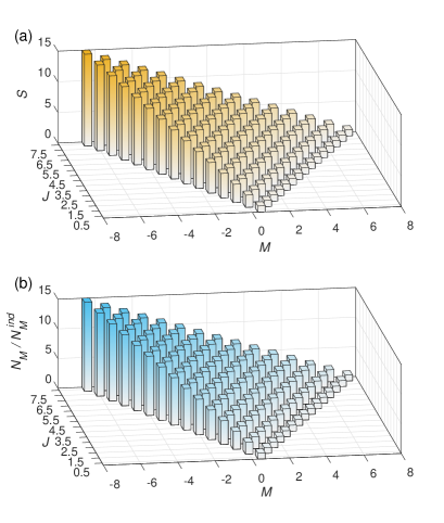
In the non-Markovian early-time regime, we calculated the normalized value of memory effects and cavity photon number with Eqs. (29) and (33) for the Dicke states of different . The results are shown in Fig. 4 where () and . It is observed that when the number of atoms is fixed, the strongest memory effects as well as photon emission happens when is 0 or next to 0, which is in agreement with Eq. (42). Interestingly, we find that the value of memory effects for the Dicke states can be fully determined by the cavity photon number in the early-time regime:
| (43) |
Considering the result in Eq. (37), there is also
| (44) |
Thus the value of memory effects can be directly measured through the atom excitation number difference or the cavity photon number. The relation Eq. (43) is proved in the following. Using the property , it is straightforward to see that
| (45) | |||||
where . Remind that the trace norm could be calculated by , where is the eigenvalue of operator . Meanwhile, the eigenvalues of is and whose absolute values sum up to 2. Therefore,
| (46) |
Considering that the normalized cavity photon number for the Dicke states is
| (47) | |||||
Eq. (43) is proved. The relation Eq. (43) demonstrates that the (change of) the cavity photon number is a fundamental reason of the memory effects in the early-time regime for the Dicke states.
We now discuss the degree of superadiance for the Dicke states in the early-time regime. The normalized cavity photon number for one independent atom in its excited state is given by by Eq. (34). Using Eq. (47), the degree of superradiance for the Dicke states could be calculated by
| (48) | |||||
for as shown in Fig. 5(a). Here the denominator represents the contribution of the emission from the independently excited atoms in . Note that the physical meaning of the denominator in Eq. (48) is different from that in Eq. (35), but their values are the same. In Fig. 5(a), for (no atom excited) are undefined and not shown. Another group of Dicke states without superradiance are (fully excited) corresponding to the right row in Fig. 5(a). Except for the two groups, other Dicke states are superradiant which could be examined by with Eq. (48). For example, for (one atom excited) represented by the left row in Fig. 5(a), there is . The single-photon superradiance is called “the greatest radiation anomaly” by Dicke. For the states in the right row in Fig. 5(a), there is for , showing a weaker degree of superradiance.
The degree of superradiance represents the magnification of the radiation intensity caused by a common environment (compared with independent environments). One interesting question is whether the memory effects are simultaneously enhanced by a common environment. To uncover the role of memory effects in the superradiance process, we next examine the degree of memory-effect-enhancement, i.e., , where is the value of memory effects with independent cavities calculated by Eq. (30). We find by mathematical induction that the value of memory effects for independently radiating atoms in a Dicke state is . Therefore, the degree of memory-effect-enhancement in the early-time regime is
| (49) |
as shown in Fig. 5(b). The enhancement of radiation intensity (caused by a common environment) is equal to the enhancement of memory effects for the Dicke states, implying that the memory effects of a common environment contribute to the establishment of superradiance.
IV.2 Factorized identical states
In this section, we investigate -atom initial states in a factorized from
| (50) |
with identical single-atom states
| (53) |
Such states are fully characterized by and and may also be superradiant. For example, states of this form are experimentally studied in Ref. [15] to realize the single-atom superradiance where a serious of atoms enter a cavity one by one. In Ref. [23], we show that such a model can be used to achieve the Heisenberg Limit in a quantum metrology scheme for measuring the atom-cavity coupling. The superradiance of two artificial atoms with initial state are experimentally observed in Ref. [17]. In the above works, the single-atom coherence () are crucial for creating superradiance. Thus it is desirable to know the influence of such states on the memory effects in superradiance, especially the role of the single-atom coherence.
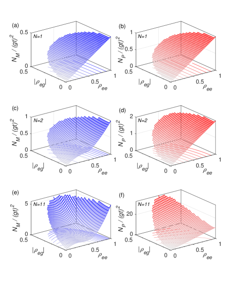
In the following, the normalized value of memory effects and the normalized cavity photon number for states described by Eq. (50) are calculated using Eqs. (29) and (33). When Eq. (53) is a pure state, i.e., , can be decomposed into the superpositions of different Dicke states [15]. Using the analytical result of in Ref. [15], we obtain the normalized cavity photon number for :
| (54) |
In contrast with Eq. (46), the analytical solution of Eq. (29) for the factorized initial states is more complicated in general. Therefore, Eq. (29) is solved numerically here. The results of the normalized and are depicted in Fig. 6 as functions of and with , 2 and . The condition are satisfied in Fig. 6 to guarantee the semipositivity of . The single-atom coherence are chosen to be real in the simulations for simplicity. Numerical results shows that the phase of does not affect the value of memory effects. Unlike the case for the Dicke states, is not proportional to in general. It is observed that the normalized value of memory effects can always be enhanced by for any . Similar situations happen for when as seen in Eq. (54) and Fig. 6 (right column). Besides, as increases, grows more and more fast with , so does . Thus we infer that for states with large , the cavity photon number are dominated by , and the memory effects are dominated by . In Fig. 6(c) and (e), it is found that the states around and tend to take lower values of memory effects compared with their neighboring states, especially when is large. This might be intuitively interpreted by the fact that and leads to a maximally mixed state of the -atom system. Besides, Fig. 6 shows that the (change of) the cavity photon number is not the only factor to determine the value of the memory effects. Other factors might include the (change of) coherence of the cavity state between the basis .
According to Eqs. (35) and (54), the degree of superradiance for is given by
| (55) | |||||
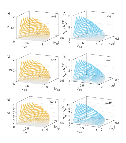
for state with . The state is superradiant when is nonzero and . Besides, the degree of superradiance grow quadratically with the single-atom coherence for . The maximum of is when and (its maximum under the semi-positivity constraint). We illustrate the degrees of superradiance for different atom numbers in Fig. 7 (left column). As done in last section, we also calculate the degree of memory-effect-enhancement in the early-time regime with Eqs. (29) and (30) for different atom numbers. These results are shown in Fig. 7 (right column). Unlike the case for the Dicke states, the dependence of on and is not the same as that of . But there are many similarities between them. When there are only one atom (), according to our definitions. For , and are slightly different, implying that the memory effects are not merely determined by the cavity photon numbers for the factorized identical states. As the atom number increases (for ), the surface shapes in the right-side figures become smoother and more similar to those in the left column, especially when is large. As shown in Fig. 7, strong memory-effect-enhancement happens for low-excitation states with high coherence (as does). Similar to Eq. (55), numerical simulations demonstrate that the maximum of is also when and . These results imply that for states with high degree of superradiance, the (enhancement of) memory effects are dominated by the cavity photon number. Besides, numerical simulations show that for initial states whose spontaneous radiation can be enhanced by a common environment (), their memory effects can always be enhanced simultaneously (). Therefore, we infer that the memory effects also contribute to the establishment of the superradiance for the factorized identical initial states.
IV.3 Other initial states
Entanglement and coherence of the initial states may play important roles in superradiance [44, 24, 25, 26, 27], especially for the Dicke states. Next, we examine the influence of the coherence (or the entanglement among the atoms) in the dephased Dicke states on the memory effects as well as the superradiance. The initial state we consider is given by
| (56) |
where . Here turns into a fully dephased state with vanishing off-diagonal elements in the basis . Meanwhile, is a mixed state of separable states whose entanglement is zero. Thus reflects the strength of entanglement or the value of coherence in . With the help of numerical solutions, we find by mathematical induction that and
| (57) | |||||
It is seen that the normalized value of memory effects increases linearly with when . The normalized cavity photon number can be calculated by Eq. (33). We obtain
| (58) | |||||
Similarly, is satisfied for the dephased Dicke states in the early-time regime.
The degree of superradiance for the dephased Dicke states can be calculated from Eq. (58) by
| (59) | |||||
for . It is observed that the entanglement or coherence (represented by ) in the depahsed Dicke state is necessary for superradiance. The degree of superradiance increases linearly with for superradiant Dicke states. Next we discuss the degree of memory-effect-enhancement caused by a common environment. When the initial state is (fully dephased), we find that . Moreover, for a partially dephased Dicke state described by Eq. (56), there is regardless of . Therefore, the degree of memory-effect-enhancement for is given by
| (60) |
as the case in Sec.IV A.
V Results in other regimes
V.1 Near-Markovian regime
In the previous sections, we investigate the superradiance and memory effect characteristics of our model in the early-time regime with quadratic expressions. The early-time dynamics can be understood by setting in Eq. (14) and consider the dynamics in a short time interval (). The definition of memory effects in Ref. [35] reflects the quality of Markovian approximation in a quantum process. Correspondingly, the initial-state-dependent memory effect in this paper reflects the quality of Markovian approximation conditioned on a particular initial state, which could be understood by . By our definition, is generally nonzero (although small) for nontrivial exact dynamics. Therefore, it could be used to investigate another interesting regime, i.e., the near-Markovian regime, by setting and considering the exact dynamics in or as least a longer time interval far beyond the environment memory time . In this section, for similar reasons, we consider the early-stage (far beyond ) dynamics in the near-Markovian regime where the system’s state does not change so much. In this way, we stress the influence of the initial states on the superradiance and the memory effects, and compare the results with those in the early-time regime. The specific scale of the early-stage time interval will be discussed in the following.
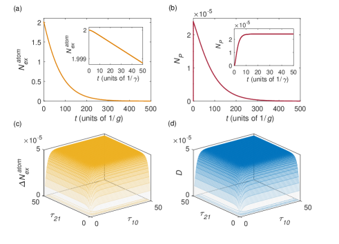
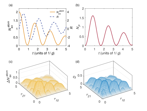
The near-Markovian dynamics of the atoms can be calculated by numerically solving Eqs. (14) or (15) and tracing out the environment under the condition . We first present a near-Markovian () example showing typical system and environment dynamics and the memory effect manifestations in Fig. 8, where 4 atoms initially in the Dicke state radiate in a common cavity. The system dynamics and environment dynamics are represented by the evolutions of the atom excitation number and the cavity photon number , respectively, as shown in Figs. 8(a) and 8((b). The memory effects are based on the trace distance of the final states in evolution A and C, i.e., which is shown in Fig. 8(d) as a function of and . Similarly, we also illustrate the difference of the atom excitation numbers denoted by as a manifestation of memory effects in Fig. 8(c).
| Characteristics | Early-time result | Characteristics | Early-stage Markovian result |
|---|---|---|---|
| Characteristics | Early-time result | Characteristics | Early-stage Markovian result |
|---|---|---|---|
As in Fig. 8, further numerical results shows that in a near-Markovian regime () with initially excited Dicke states or factorized identical states, the cavity photon number first experiences a rapid increase before and then reaches a plateau while the atom emission rate is almost constant as shown in the insets of Figs. 8(b) and 8(a). After the plateau, evolves on a larger timescale given by where may monotonically decay for a highly superradiant initial state, or first increase and then decay, for a less superradiant one. Thus the early stage of a near-Markovian dynamics in our work could be understood as a time interval where . Here is the lifetime of the radiation that is found to be proportional to and initial-state-dependent. In other words, in the early stage of a near-Markovian dynamics, the environment photon number and the atom emission rate becomes almost steady while the system does not change so much. Therefore, the almost-steady cavity photon number , as shown by the plateau in the inset of Fig. 8(b), represents the typical cavity photon number during the early stage of a near-Markovian process. In the near-Markovian regime, the memory effects can be calculated by Eq. (11) where . Numerical evidences imply that there exists only one local maximum of when and are optimized (at least) in the early stage of a near-Markovian dynamics. For example, in Fig. 8, the optimal and are about in . In contrast, the optimal and that maximizing might be beyond the early-stage time interval for a less superadiant initial state. However, in practice, the values of as well as in the early stage of a near-Markovian dynamics are nearly steady and robust against and after , especially when is large. This makes it easy to define and numerically calculate the near-steady value of the excitation number difference .
We now discuss quantitatively the characteristics of the superadiance and the memory effects of the early-stage dynamics in near-Markovian regime. In Fig. 8, there are and , where is the photon emission rate of the atoms. Meanwhile, the difference of cavity photon number in Fig. 8(c) and the trace distance in Fig. 8(d) are approximately the same. This implies that the difference of excitation numbers can be used to measure the memory effects for the Dicke states instead of the trace distance for simplicity. Further simulations imply that and as goes larger and larger (the Markovian limit). For example, for , there are and for the same time interval as in Fig. 8.
Inspired by the above results, we conducted a number of simulations in the near-Markovian regime (with different ) where the initial states included the (dephased) Dicke states with different , , and , and the factorized identical states with different , , and . As in former sections, we find that the characteristics of superradiance and memory effects in the early stage of a near-Markovian dynamics can be well approximated by analytic expressions. These characteristics include the steady cavity photon number of a common cavity () and independent cavities (), the value of memory effects for a common cavity () and independent cavities (), the degree of superradiance , and the degree of memory-effect-enhancement . Using instead of for formal correspondence, these early-stage characteristics of the superradiance and the memory effects in the near-Markovian regime are listed in Table 1 (dephased Dicke states) and 2 (factorized identical states) and compared with the early-time results. As shown in Table 1 and 2, the relations between the early-stage Markovian results and the early-time results can be summarized by
| (62) | |||||
| (63) |
for both collective and independent radiations and the two types of initial states. Therefore, the degree of superradiance in the early stage of a Markovian regime is consistent with that in the early-time regime, so does the degree of memory-effect-enhancement . Besides, for the Dicke states, there are and in the early stage of the near-Markovian dynamics. In comparison, for the factorized identical states, the following relations holds approximately in the early stage of the near-Markovian dynamics: and . The results in this section demonstrate that the characteristics of memory effects and superradiance in the early stage of a near-Markovian dynamics can be well reflected by its early-time dynamics.
V.2 Strongly non-Markovian regime
In this section, we continue to discuss the influence of the initial states on the superradiance and memory effects in a strongly non-Markovian regime where and is comparable and are considered. In this regime, typically there are backflows of photons from the cavity to the atoms and the values of memory effects are much higher than those in the early-time regime or the near-Markovian regime. It is worth noting that, in this regime, the superradiance characteristics, such as the atom emission rate and the cavity photon number , are neither quadratic nor steady in time. Therefore, we may discuss their maxima (denoted by and ) and use as the degree of superradiance. Moreover (unlike what happens in other regimes), the initial states usually have evolved dramatically when the atom emission rate or other quantities reach their maxima.
As in last section, we provide a typical example in Fig. 9 showing the dynamics of the atoms and one common cavity as well as the memory effect manifestations in a strongly non-Markovian regime with . The results are obtained by numerically solving Eqs. (14) and (15). The initial state is the same as that in Fig. 8. As shown in Fig. 9(a), there are backflows of photons from the cavity to the atoms and the maximal atoms emission rate happens during the first emission pulse. Besides, the maximal cavity photon number happens at the end of the first emission pulse as shown in Fig. 9(b). The trace distance as a function of and are shown in Fig. 9(d) where , implying that the dynamics is far from Markovian. Figure 9(d) also demonstrate that the optimal and for the global maximum of can be found in a limited time interval. The manifestation of memory effects by as a function of and is shown in Fig. 9(c). Although the surface shapes in Figs. 9(c) and 9(d) are similar, the value of are not bounded as is. Further simulations with other initially excited Dicke states and factorized identical states (with ) show similar results as shown in Fig. 9, e.g., there are backflows of photons and () happens during (after) the first emission pulse. Thus the degree of superradiance can be clearly defined in our simulations.
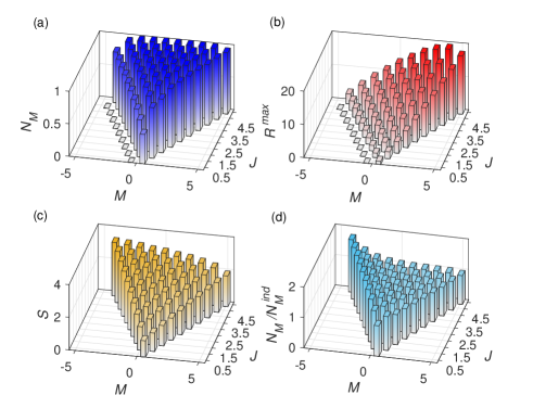
We numerically calculated the value of memory effects , the maximal atom emission rate , the degree of superradiance and the degree of memory-effect-enhancement for the Dicke states and the factorized identical states with . The results for the Dicke states are shown in Fig. 10 with no more than atoms. In the strongly non-Markovian regime, the values of memory effect are close to 1 for most of the Dicke states as shown in Fig. 10(a), implying that the Markovian approximation are invalid for their dynamics. Unlike the results in the early-time regime or in the near-Markovian regime, is not proportional to here. The first reason is that it tends to saturate () for highly non-Markovian dynamics. The second reason is as follows: on the timescale of the optimal () that maximizing , the initial states have evolved dramatically. Thus the connection between and is weaker compared with those in the other two regimes we discussed. However, the dependence of on and is still roughly similar to that in Fig. 4. For example, for a fixed , the strongest memory effects happens for or near 0. In the strongly non-Markovian regime, the radiation intensity is represented by the maximal emission rate as shown in Fig. 9(a) (dashed line). For , the state have the strongest emission intensity with a given . As increases, the states with the strongest emission intensity become as shown in Fig. 9(b). We infer that a large , the Dicke states with might be the most radiative ones. Compared with the results in Fig. 4, the Dicke states with small and large are more radiative than those with . The reason is as mentioned before, i.e., the states with large may have evolved to more superradiant ones when happens. Figures 10(c) and 10(d) show the degree of superradiance and the degree of memory-effect-enhancement. They are not proportional to as in Fig. 5 in this regime. However, the highest degree of superradiance as well as memory-effect-enhancement in Figs. 10(c) and 10(d) still happens for the state with the largest and . Other simulations show that, for the Dicke state (one excitation) in a common cavity, the memory effects for the dephased Dicke states satisfies , i.e., increases linearly with . For other Dicke states, this relation holds approximately at least for a few atoms.
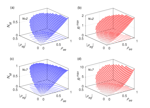
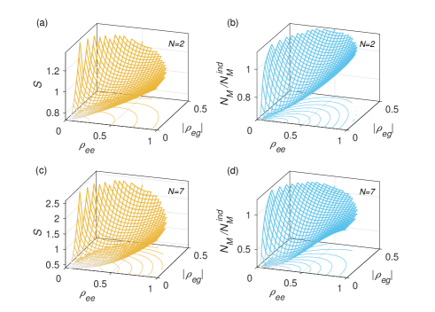
The value of memory effects and the maximal atom emission rate for the factorized identical states are shown in Fig. 11 with two and seven atoms as functions of and . In the strongly non-Markovian regime, the population , the coherence and the atom number can increase the memory effects as well as the maximal atom emission rate. The results show some resemblance to those in Fig. 6 but with stronger memory effects and emission intensities in general. When is small, the memory effects are still weak as the system almost stays in its ground state, which can be approximated by a Markovian dynamics in a trivial sense. The degree of superradiance and the degree of memory-effect-enhancement are shown in Fig. 12. In contrast with the results in Fig. 7, may be greater (less) than 1 for states with . Because when or happen, these initial states may evolve to more (less) superradiant ones. Similarly, may also be less than 1 in the strongly non-Markovian regime. However, as in Fig. 7, the coherence can still increase the degree of superradiance, and initial states with low-excitations and strong coherence have large values of and . Besides, the surface shapes in Fig. 12 (right column) are roughly similar to those in Fig. 12 (left column). Other calculations demonstrate that, for both and as initial states, the following relation holds roughly: in our simulations. Considering the weaker connection between the discussed characteristics and the initial states, we may say that the results in the strongly non-Markovian regime are consistent with those in the early-time regime.
VI Discussions and Conclusions
In this paper, we propose a method to evaluate the memory effects in a quantum process conditioned on a particular system initial state. The method is based on the physical interpretations of the inequality [35]. Some features of the non-Markovianity measure in Ref. [35] are inherited. For example, nonzero memory effects can be characterized even in regimes where nonmonotonic behaviors do not occur, or have not occurred yet. Besides, is satisfied without additional normalizations. This allows us to compare the memory effects of quantum systems with different dimensions (e.g., different numbers of atoms in our model). Using our method, we calculate the influence of two types of initial states on the memory effects as well as the superradiance in different regimes. The characteristics of the memory effects and the superradiance are compared to reveal the role of memory effects in superradiance, and conversely, to understand the physical sources of the memory effects.
In the early-time (Zeno) regime and the (early-stage) near-Markovian regime where the initial states do not change so much, the main observations and conclusions are as follows. The memory effects for the (dephased) Dicke states are fully determined by the cavity photon number (connected to the atom radiation intensity) and they are proportional to for quadratic dynamics, or in the Markovian limit. Meanwhile, the degree of superradiance is equal to the degree memory-effect-enhancement (from independent radiation to collective radiation) given by . For the factorized identical states, the memory effects, the radiation intensity and the degree of superradiance can all be enhanced by the single-atom coherence. The memory effects are closely related to the cavity photon number, meanwhile, the superradiance () of an initial state is accompanied by the enhancement of memory effects (by a common cavity). These results demonstrate that the memory effects are closely related to the radiation intensity. Correspondingly, the enhancement of memory effects by a common environment plays an important role on the establishment of superradiance, especially for the Dicke states. On the other hand, these results imply that the (change of) cavity photon number is one fundamental source of memory effects, especially for the Dicke states. Besides, the entanglement in the Dicke states and the single-atom coherence in the factorized identical state are necessary for the existence of superradiance and important for the memory-effect-enhancement.
For the whole dynamics in a strongly non-Markovian regime, an initial state may evolves dramatically during the radiation lifetime, making its influence weaker. However, simulations demonstrate that the relationships between the radiation intensity (degree of superradiance) and the memory effects (memory-effect-enhancement) are basically consistent with those in the other two regimes. The results in different regimes demonstrate that the characteristics of memory effects and superradiance in long-time dynamics can be reflected by its early-time behaviours. In addition, our work also provides other ways to measure the memory effects through the atom excitation number or the cavity photon number.
VII ACKNOWLEDGMENTS
The authors thank X. L. Huang, X. L. Zhao, J. Cheng and B. Cui for helpful discussions. The work is supported by the National Natural Science Foundation of China under Grant No. 11705026, the Fundamental Research Funds for the Central Universities in China under Grant No. 3132020178 and the Natural Science Foundation of Liaoning Province under Grant No. 2023-MS-333.
References
- [1] S. Cordero and G. García–Calderón, Analytical study of quadratic and nonquadratic short-time behavior of quantum decay, Phys. Rev. A 86, 062116 (2012).
- [2] S. Wenderoth, H.-P. Breuer, and M. Thoss, Quantifying the influence of the initial state on the dynamics of an open quantum system, Phys. Rev. A 107, 022211 (2023).
- [3] Á. Rivas, S. F. Huelga, and M. B. Plenio, Quantum non-Markovianity: Characterization, quantification and detection, Rep. Prog. Phys. 77, 094001 (2014).
- [4] H.-P. Breuer, E.-M. Laine, J. Piilo, and B. Vacchini, Colloquium: Non-Markovian dynamics in open quantum systems, Rev. Mod. Phys. 88, 021002 (2016).
- [5] I. de Vega and D. Alonso, Dynamics of non-Markovian open quantum systems, Rev. Mod. Phys. 89, 015001 (2017).
- [6] L. Li, M. J. W. Hall, and H. M. Wiseman, Concepts of quantum non-Markovianity: A hierarchy, Phys. Rep. 759, 1 (2018).
- [7] R. H. Dicke, Coherence in spontaneous radiation processes, Phys. Rev. 93, 99 (1954).
- [8] A. V. Andreev, V. I. Emel’yanov, and Y. A. Il’inskiĭ, Collective spontaneous emission (Dicke superradiance), Sov. Phys. Usp. 23, 493 (1980).
- [9] N. E. Rehler and J. H. Eberly, Superradiance, Phys. Rev. A 3, 1735 (1971).
- [10] M. Gross and S. Haroche, Superradiance: An essay on the theory of collective spontaneous emission, Phys. Rep. 93, 301 (1982).
- [11] G. S. Agarwal, Master-Equation Approach to Spontaneous Emission, Phys. Rev. A 2, 2038 (1970).
- [12] B. Bonifacio, P. Schwendimann, and F. Haake, Quantum statistical theory of superradiance. I, Phys. Rev. A 4, 302 (1971).
- [13] B. Bonifacio, P. Schwendimann, and F. Haake, Quantum statistical theory of superradiance. II, Phys. Rev. A 4, 854 (1971).
- [14] H. J. Carmichael, Statistical methods in quantum optics 1: master equations and Fokker-Planck equations (Springer, Berlin, 1999).
- [15] J. Kim, D. Yang, S. Oh, and K. An, Coherent single-atom superradiance, Science 359, 662 (2018).
- [16] M. O. Scully and A. A. Svidzinsky, The super of superradiance, Science 325, 1510 (2009).
- [17] J. A. Mlynek, A. A. Abdumalikov, C. Eichler, and A. Wallraff, Observation of Dicke superradiance for two artificial atoms in a cavity with high decay rate, Nat. Commun. 5, 5186 (2014).
- [18] A. Rastogi, E. Saglamyurek, T. Hrushevskyi, and L. J. LeBlanc, Superradiance-Mediated Photon Storage for Broadband Quantum Memory, Phys. Rev. Lett. 129, 120502 (2022).
- [19] F. Robicheaux, Theoretical study of early-time superradiance for atom clouds and arrays, Phys. Rev. A 104, 063706 (2021).
- [20] D. Mogilevtsev, E. Garusov, M. V. Korolkov, V. N. Shatokhin, and S. B. Cavalcanti, Restoring the Heisenberg limit via collective non-Markovian dephasing, Phys. Rev. A 98, 042116 (2018).
- [21] M. Bojer and J. von Zanthier, Dicke-like superradiance of distant noninteracting atoms, Phys. Rev. A 106, 053712 (2022).
- [22] V. Paulisch, M. Perarnau-Llobet, A. González-Tudela, and J. I. Cirac, Quantum metrology with one-dimensional superradiant photonic states, Phys. Rev. A 99, 043807 (2019).
- [23] W. Cheng, S. C. Hou, Z. Wang, and X. X. Yi, Phys. Rev. A 100, 053825 (2019).
- [24] K. C. Tan, S. Choi, H. Kwon, and H. Jeong, Coherence, quantum Fisher information, superradiance, and entanglement as interconvertible resources, Phys. Rev. A 97, 052304 (2018).
- [25] E. Wolfe and S. F. Yelin, Certifying Separability in Symmetric Mixed States of N Qubits, Phys. Rev. Lett. 112, 140402 (2014).
- [26] M. E. Tasgin, Many-Particle Entanglement Criterion for Superradiantlike States, Phys. Rev. Lett. 119, 033601 (2017).
- [27] F. Lohof, D. Schumayer, D. A. W. Hutchinson, and C. Gies, Signatures of Superradiance as a Witness to Multipartite Entanglement, Phys. Rev. Lett. 131, 063601 (2023).
- [28] F. Dinc and A. M. Brańczyk, Non-Markovian super-superradiance in a linear chain of up to 100 qubits, Phys. Rev. Research 1, 032042(R) (2019).
- [29] K. Sinha, P. Meystre, E. A. Goldschmidt, F. K. Fatemi, S. L. Rolston, and P. Solano, Non-Markovian collective emission from macroscopically separated emitters, Phys. Rev. Lett. 124, 043603 (2020).
- [30] Q-.Y. Qiu, Y. Wu, and X-.Y. Lü, Collective radiance of giant atoms in non-Markovian regime, Sci. China Phys. Mech. Astron. 66, 224212 (2023).
- [31] Y. X. Zhang, Zeno regime of collective emission: Non-Markovianity beyond retardation, Phys. Rev. Lett. 131, 193603 (2023).
- [32] H.-P. Breuer, E.-M. Laine, and J. Piilo, Measure for the Degree of Non-Markovian Behavior of Quantum Processes in Open Systems, Phys. Rev. Lett. 103, 210401 (2009).
- [33] Á. Rivas, S. F. Huelga, and M. B. Plenio, Entanglement and Non-Markovianity of Quantum Evolutions, Phys. Rev. Lett. 105, 050403 (2010).
- [34] D. Chruściński and A. Kossakowski, Non-Markovian Quantum Dynamics: Local versus Nonlocal, Phys. Rev. lett. 104, 070406 (2010).
- [35] S. C. Hou, S. L. Liang, and X. X. Yi, Non-Markovianity and memory effects in quantum open systems, Phys. Rev. A. 91, 012109 (2015).
- [36] Á. Rivas and S. F. Huelga, Open Quantum Systems An Introduction (Springer, Heidelberg, 2012).
- [37] S. C. Hou, X. X. Yi, S.X.Yu, and C.H.Oh, Alternative non-Markovianity measure by divisibility of dynamical maps, Phys. Rev. A 83, 062115 (2011).
- [38] M.-D. Choi, Completely positive linear maps on complex matrices, Lin. Alg. and Appl. 10, 285 (1975).
- [39] A. Jamiołkowski, Linear transformations which preserve trace and positive semidefiniteness of operators, Rep. Math. Phys. 3, 275 (1972).
- [40] P. Facchi, H. Nakazato, and S. Pascazio, From the quantum Zeno to the inverse quantum Zeno effect, Phys. Rev. Lett. 86, 2699 (2001).
- [41] L. S. Schulman, Observational line broadening and the duration of a quantum jump, J. Phys. A 30, L293 (1997);
- [42] A. Crespi, F.V. Pepe, P. Facchi, F. Sciarrino, P. Mataloni, H. Nakazato, S. Pascazio, and R. Osellame, Experimental investigation of quantum decay at short, intermediate and long times via integrated photonics, Phys. Rev. Lett. 122, 130401 (2019).
- [43] W. Wu and H.-Q. Lin, Quantum Zeno and anti-Zeno effects in quantum dissipative systems, Phys. Rev. A 95, 042132 (2017).
- [44] G. S. Agarwal, Quantum Optics (Cambridge University Press, Cambridge, 2013).