Influence of pulsatile blood flow on allometry of aortic wall shear stress

In the case of a Poiseuille flow, shear stress on the wall is worth:

$$\tau=2\mu\frac{u_{max}}{a}$$

(1)

Let us detail the allometric arguments of equation 1, applied to the aortic artery:

• •

  the aortic diameter $a$ is assumed to vary as $M^{0.375}$, both from theoretical ([5]) and experimental considerations ([3] and [4])

• •

  the dynamic viscosity of blood $\mu$ is assumed to be independent of the body mass

• •

  the aortic velocity $u_{max}$ can be seen as the cardiac flow rate divided the aortic cross-section $u_{max}=\frac{Q}{\pi a^{2}}$. The cardiac flow rate varies with $M^{0.75}$, as described in [5] and [6]. Therefore, $u_{max}$ is independent of $M$.

We can conclude that in the case of a Poiseuille flow, wall shear stress scales as:

$$\tau_{Poiseuille}\propto M^{-0.375}$$

(2)

Additionally, we can deduce the allometry of temporal gradient of wall shear stress. Since $\frac{\partial\tau}{\partial t}\sim\omega\tau$, $\omega\sim M^{-0.25}$ being the cardiac frequency, we get:

$$\frac{\partial\tau}{\partial t}_{Poiseuille}\sim M_{b}^{-0.625}$$

(3)

We obtain the following values for mice, rabbits and humans (tab. 1), as described in [2], relatively to the human value:

We consider a purely oscillating pressure gradient (eq. 5) in the same geometry, and derive the allometry of wall shear stress, temporal gradient of wall shear stress and peak velocity associated to this flow.

In reality, the pressure gradient is neither steady, nor purely oscillatory. It was shown ([13], [14]) that the pressure gradient $\nabla P$ could be reasonably approximated by the first six harmonics of its Fourier decomposition. In our case, six harmonics are not needed, as we are only looking at allometric variations. Along with the allomerty of the Womersley flow (first harmonic), we will present the sum of Poiseuille and Womersley flows (fundamental + first harmonic), which we denote PW flow from here on:

$$u_{PW}=u_{Poiseuille}+u_{Womersley}$$

(15)

Consequently, by linearity of differentiation, wall shear stress and its temporal gradient are obtained by: $\tau_{PW}=\tau_{Poiseuille}+\tau_{Womersley}$ and $\nabla\tau_{PW}=\nabla\tau_{Poiseuille}+\nabla\tau_{Womersley}$. Concerning peak velocity however, calculations are done using the total velocity field $u_{PW}$.

To evaluate the allometry of wall shear stress, we need to know the allometry of every variable present in its expression. Concerning $a$, $\alpha$ or $\omega$, the allometry is known from [2], as summed up in table 5. But the allometry of $G_{1}$ is unknown. To overcome this problem, we substitute the flow rate $Q$, which follows an experimentally determined allometry $Q\sim M^{0.75}$. This step can be discussed, since the Womersley flow model implies a zero average flow rate. Although $<Q>$, the time average value of Q, is always null, its effective value $<Q^{2}>$ is indeed an increasing function of body mass, which justifies the use of $Q\propto M^{0.75}$ in the Womersley model. Combining (12) and (14), we obtain

$$\underline{\tau}=\frac{\omega\rho J_{1}(x)}{\pi ai(xJ_{0}(x)-2J_{1}(x))}\underline{Q}$$

(16)

with $x=i^{\frac{3}{2}}\alpha$ and $\underline{Q}$, $\underline{\tau}$ the complex variables such that $Q=\Re(\underline{Q})$ and $\tau=\Re(\underline{\tau})$.
We introduce the following function $f$, such that $\underline{\tau}=\frac{\omega\rho}{\pi a}f(\alpha)\underline{Q}$:

$$f(\alpha)=\frac{iJ_{1}(x)}{(2J_{1}(x)-xJ_{0}(x))}$$

(17)

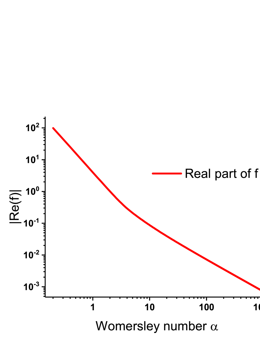
We plot $|\Re(f)|$ as a function of $\alpha$ in logarithmic scale on figure 1). Note that $\Re(f)$ is negative, ie $|\Re(f)|=-\Re(f)$.

• •

  for $\alpha<2$, $\Re(f)\sim\alpha^{-2}$ ($r^{2}=0.98$)

• •

  for $\alpha>5$, $\Re(f)\sim\alpha^{-1}$ ($r^{2}=0.99$)

We can confirm these regressions using Taylor and asymptotic developments of $J_{0}$ and $J_{1}$:

$$J_{0}(x)=1-x^{2}/4+O_{0}(x^{4})$$

(18)

and

$$J_{1}(x)=x/2-x^{3}/16+O_{0}(x^{5})$$

(19)

using big O notation ([16], p. 687).
Consequently, for $\alpha<<1$, $f(\alpha)\ \approx\ 4i/x^{2}\approx-4/\alpha^{2}$, which confirms $\Re(f)\sim\alpha^{-2}$ for $\alpha<<1$.
Conversely, for $|x|\rightarrow+\infty$:

$$J_{0}(x)\approx\sqrt{\frac{2}{\pi x}}cos(x-\pi/4)$$

(20)

and

$$J_{1}(x)\approx\sqrt{\frac{2}{\pi x}}sin(x-\pi/4)$$

(21)

introducing complex sine and cosine ([16], p. 723).
In our case, $x=i^{3/2}\alpha=\alpha\exp(3i\pi/4)$, therefore $f(\alpha)\approx-\frac{itan(x)}{x}=\frac{tanh(\alpha\sqrt{2}/2)}{\alpha}\exp(-3i\pi/4)$ and finally $\Re(f(\alpha))\approx\frac{\sqrt{2}}{2\alpha}$, which confirms $\Re(f)\sim\alpha^{-1}$ for $\alpha\rightarrow\infty$.
Knowing that $\alpha\sim M^{0.25}$, and that $\frac{\omega\rho Q}{\pi a}\sim M^{0.125}$ (see table 5 at the end of the document), we obtain:

$\tau_{womersley}\sim M^{-0.375}$ for $M<1\ kg$ and $\tau_{womersley}\sim M^{-0.125}$ for $M>10\ kg$

which differs notably from

$\tau_{poiseuille}\sim M^{-0.375}$ for all $M$

We can complete the previous chart of relative shear stress for different animals (tab. 2).

We also plot the compared shear stress induced by a Poiseuille, Womersley or physiological PW flows as a function of mass on figure 2.

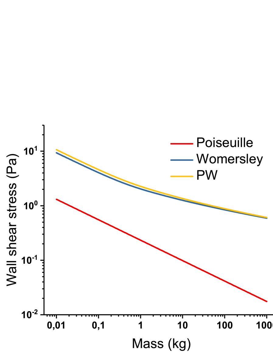
First of all, we can see that despite several allometric approximations (flow rate, heart rate, aortic radius, Womersley number), the absolute value of wall shear stress $\tau\in[0.1;10]\ Pa$ is within the range of measured values ([12], ch. , p.502). We observe that Poiseuille shear stress is, in absolute value, much lower than Womersley stress (10 to 20 times lower as mass increases). At low masses ($M<1\ kg$), both flows follow the same allometry: $\tau_{PW}\propto M^{-0.375}$. At higher masses however, ($M>10\ kg$), the Womersley stress accounts for the variations of total stress and thus $\tau_{PW}\propto M^{-0.125}$. In practice, it means that the difference in wall shear stress between mice and men is greatly reduced by the influence of pulsatile flow in larger arteries, and shows the necessity of the unsteady modeling of blood flow for correct body mass allometries.

Concerning the temporal gradient of shear stress, we get $\frac{\partial\tau}{\partial t}\sim\omega\tau$, with $\omega\sim M^{-0.25}$ [2], and therefore:

$\frac{\partial\tau}{\partial t}_{wom}\sim M_{b}^{-0.625}$ for $M<1\ kg$ and $\frac{\partial\tau}{\partial t}_{wom}\sim M_{b}^{-0.375}$ for $M>10\ kg$

Which should be compared to

$\frac{\partial\tau}{\partial t}_{poi}\sim M^{-0.625}$ for all $M$

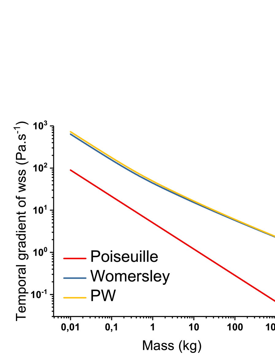
We compare the values of shear stress gradient between Womersley and Poiseuille in tab. 3. Poiseuille TGWSS is lower than Womersley TGWSS, and the allometric domination at high masses is also present. The graph of these functions (fig. 3) is very similar to the one on wall shear stress (fig. 2). At low masses ($M<1kg$), both flows result in $\frac{\partial\tau}{\partial t}_{PW}\propto M^{-0.625}$ allometry, and at higher masses ($M>10kg$), Womersley stresses dominate the allometry: $\frac{\partial\tau}{\partial t}_{PW}\propto M^{-0.375}$. Here again, we observe a reduced difference between men and mice due to the influence of unsteady flow at high Womersley numbers.

And finally, we can express the maximum velocity. First we inject the expression of the flow rate in the Womersley velocity to absorb the time dependence (again using $x=i^{3/2}\alpha$) :

$$u_{Wom}(r)=\frac{Q}{\pi a^{2}}\times\frac{J_{0}(xr/a)-J_{0}(x)}{xJ_{0}(x)-2J_{1}(x)}$$

(22)

We know that $\frac{Q}{\pi a^{2}}$ is independent of $\alpha$ (table 5), therefore

$$u^{Wom}_{max}(\alpha)\propto\max_{r\in[0,a]}\Re\Bigg{(}\frac{J_{0}(xr/a)-J_{0}(x)}{xJ_{0}(x)-2J_{1}(x)}\Bigg{)}=\max_{r\in[0,a]}(g_{wom}(\alpha))$$

(23)

Recalling equivalents of $J_{0}$ and $J_{1}$ (eq. 18 to 21), we can find equivalents of $g_{wom}(\alpha)$ at low and high $\alpha$:

• •

  for $M<<1$, $g_{wom}\ \sim\frac{\sqrt{2}}{2\alpha}\sim M^{-0.25}$, we observe a divergence:

  $$\lim_{M\to 0}u^{Wom}_{max}=+\infty$$

  .

• •

  for $M>>1$, we also obtain $g_{wom}\ \sim\frac{1}{\alpha}\sim M^{-0.25}$, and

  $$\lim_{M\to+\infty}u^{Wom}_{max}=0$$

  .

We plot $\max_{r}(g_{wom})$, which represents the Womersley peak velocity only, as a function of M on figure 4. We also add the Poiseuille peak velocity.
Concerning PW flow, calculations must be done considering the total velocity field: recalling the expression of $u_{Pois}$ as a function of $Q$ and $r$: $u_{Pois}=\frac{2Q}{\pi a^{2}}(1-\frac{r}{a})$, $u^{PW}_{max}$ is:

$$u^{PW}_{max}(\alpha)\propto\max_{r\in[0,a]}\Re\Bigg{(}2(1-\frac{r}{a})+\frac{J_{0}(xr/a)-J_{0}(x)}{xJ_{0}(x)-2J_{1}(x)}\Bigg{)}=\max_{r\in[0,a]}(g_{PW}(\alpha))$$

(24)

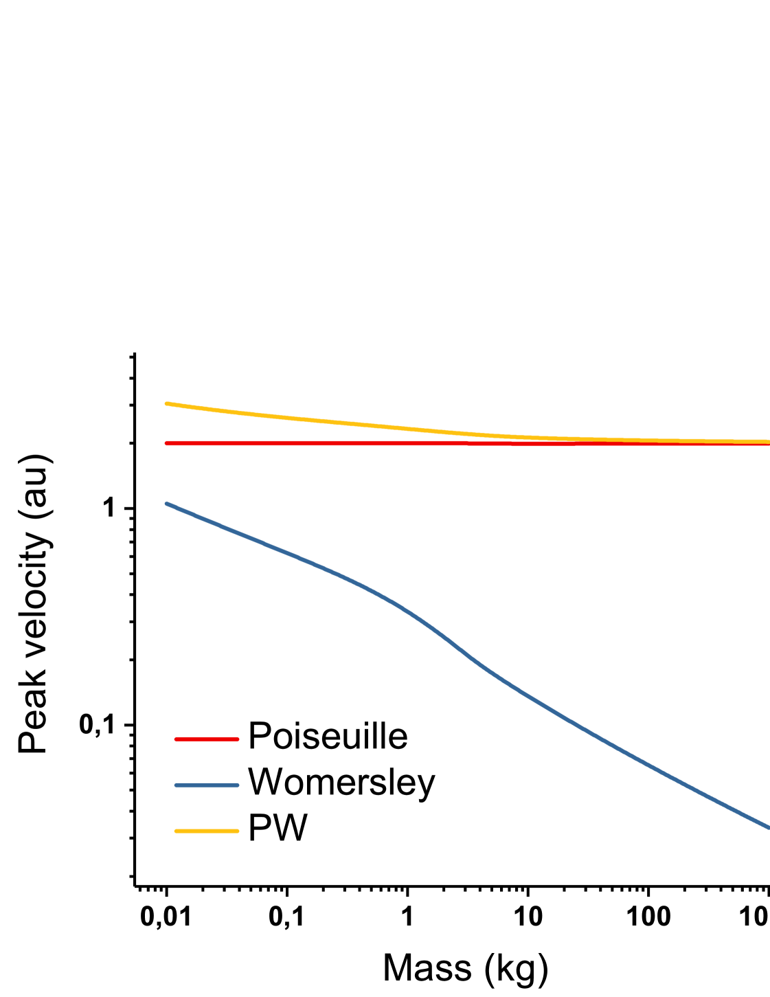
On figure 4, we can see that the Womersley flow alone gives rise to a peak velocity which vanishes with $M$ (blue curve), while the PW flow (yellow curve) shows a constant peak velocity for reasonably high $M$. This proves that the constant peak velocity measured experimentally [18] is due to the steady Poiseuille component of the flow, rather than to the Womersley unsteady component. We also observe that the maximum velocity is systematically reached in the center of the artery ($r=0$, data not shown), which is not the case for a pure Womersley flow at high Womersley number. This confirms the domination of the Poiseuille flow. Figure 4 further proves the necessity of a combined Poiseuille - Womersley flow to account for the variations of the different hemodynamic parameters.

We summarize the different allometries obtained throughout this work in table 4.

References

- [1] Cunningham KS., Gotlieb AI., The role of shear stress in the pathogenesis of atherosclerosis Lab Invest. 2005 Jul;85(7):942
- [2] P. Weinberg, C. Ethier, Twenty-fold difference in hemodynamic wall shear stress between murine and human aortas. Journal of Biomechanics 40, 2007
- [3] Clark, A.J., Comparative physiology of the heart MacMillan, New-York, 1927
- [4] Holt, J.P., Rhode, E.A., Holt, W.W., Kines, H. Geometric similarities of aortas, venae cavae and certain of their branches in mammals American Journal of Physiology Regulatory, Integrative and Comparative Physiology 241, 1981
- [5] West, G.B., Brown, J.H., Enquist, B.J.. A general model for the origin of allometric scaling laws in biology Science 276, 1997
- [6] Kleiber, M., Body size and metabolism Hilgardia 6, 315-353, 1932
- [7] Castier, Y., Brandes, R.P., Leseche, G., Tedgui, A., Lehoux, S. 2005 p47phox-dependent NADPH oxidase regulates flow-induced vascular remodeling Circulation Research 97, 533-540, 2005
- [8] Ibrahim, J., Miyashiro, J.K., Berk, B.C., Shear stress is differentially regulated among inbred rat strains Circulation Research 92, 1001–1009, 2003
- [9] Lacy, J.L., Nanavaty, T., Dai, D., Nayak, N., Haynes, N., Martin, C., Development and validation of a novel technique for murine first-pass radionuclide angiography with a fast multiwire camera and tantalum 178 Journal of Nuclear Cardiology 8, 171–181, 2001
- [10] Khir, A.W., Henein, M.Y., Koh, T., Das, S.K., Parker, K.H., Gibson, D.G., Arterial waves in humans during peripheral vascular surgery Clinical Science (London) 101, 749–757, 2001
- [11] J. Mestel Pulsatile flow in a long straight artery Lecture 14, Biofluid Mechanics, Imperial College, 2009
- [12] W. Nichols, M. O’Rourke, C. Vlachopoulos, A. Hoeks, R. Reneman - McDonald’s blod flow in arteries - Sixth edition - Chapter 10 - Contours of pressure and flow waves in arteries
- [13] Tracy Morland - Gravitational Effects On Blood Flow - Mathematical Biology group, University of Colorado at Boulder, available at mathbio.colorado.edu/index.php/MBW:Gravitational_Effects_on_Blood_Flow
- [14] J.R. Womersley - Method for the calculation of velocity, rate of flow and viscous drag in arteries when the pressure gradient is known - Journal of Physiology (I955) 127, p. 553-563
- [15] C. Cheng & al. - Review: Large variations in wall shear stress levels within one species and between species - Atherosclerosis, December 2007, Volume 195, Issue 2, Pages 225–235
- [16] G. Arfken, H. Weber - Mathematical methods for physicists, sixth edition - Elsevier Acedemic Press, 2005
- [17] J. Greve & al. - Allometric Scaling of Wall Shear Stress from Mouse to Man: Quantification Using Cine Phase-Contrast MRI and Computational Fluid Dynamics - American Journal of Physiology - Heart and Circulatroy Physiology, May 19, 2006
- [18] K. Schmidt-Nielsen - Scaling — Why is Animal Size so Important? - Cambridge University Press, Cambridge 1984
- [19] Greve et al. Allometric scaling of wall shear stress from mice to humans quantification using cine phase-contrast MRI and computational fluid dynamics Am. J. Physiol. Heart. Circ. Physiol. 291, 2006