Information bottleneck theory of high-dimensional regression: relevancy, efficiency and optimality
Abstract
Avoiding overfitting is a central challenge in machine learning, yet many large neural networks readily achieve zero training loss. This puzzling contradiction necessitates new approaches to the study of overfitting. Here we quantify overfitting via residual information, defined as the bits in fitted models that encode noise in training data. Information efficient learning algorithms minimize residual information while maximizing the relevant bits, which are predictive of the unknown generative models. We solve this optimization to obtain the information content of optimal algorithms for a linear regression problem and compare it to that of randomized ridge regression. Our results demonstrate the fundamental trade-off between residual and relevant information and characterize the relative information efficiency of randomized regression with respect to optimal algorithms. Finally, using results from random matrix theory, we reveal the information complexity of learning a linear map in high dimensions and unveil information-theoretic analogs of double and multiple descent phenomena.
1 Information bottleneck
Conventional wisdom identifies overfitting as being detrimental to generalization performance, yet modern machine learning is dominated by models that perfectly fit training data. Recent attempts to resolve this dilemma have offered much needed insight into the generalization properties of perfectly fitted models [1, 2]. However investigations of overfitting beyond generalization error have received less attention. In this work we present a quantitative analysis of overfitting based on information theory and, in particular, the information bottleneck (IB) method [3].
The essence of learning is the ability to find useful and generalizable representations of training data. An example of such a representation is a fitted model which may capture statistical correlations between two variables (regression and pattern recognition) or the relative likelihood of random variables (density estimation). While what makes a representation useful is problem specific, a good model generalizes well—that is, it is consistent with test data even though they are not used at training.
Achieving good generalization requires information about the unknown data generating process. Maximizing this information is an intuitive strategy, yet extracting too many bits from the training data hurts generalization [4, 5]. This fundamental trade-off underpins the IB principle, which formalizes the notion of a maximally efficient representation as an optimization problem [3]111Note that this minimization is identical to that of the original IB method since under the Markov constraint .
| (1) |
Here denotes the data generating process. The conditional distribution denotes a learning algorithm which defines a stochastic mapping from the training data to the hypothesis or fitted model (Fig 1a). The relevant information, , is the bits in that are informative of the generative model . On the other hand, the residual information, , is the bits in that are specific to each realization of the training data and thus are not informative of . In other words the residual bits measure the degree of overfitting. The parameter controls the trade-off between these two informations.
The IB method has found success in a diverse array of applications, from neural coding [6, 7], developmental biology [8] and statistical physics [9, 10, 11] to clustering [12], deep learning [13, 14, 15] and reinforcement learning [16].
Indeed the IB principle has emerged as a potential candidate for a unifying framework for understanding learning phenomena [17, 18, 15, 19] and a number of recent works have explored deep connections between information-theoretic quantities and generalization properties [4, 20, 5, 21, 22, 23, 24, 25, 26, 27, 28]. However a direct application of information theory to practical learning algorithms is often limited by the difficulty in estimating information, especially in high dimensions. While recent advances in characterizing variational bounds of mutual information have enabled a great deal of scalable, information-theory inspired learning methods [13, 29, 30], these bounds are generally loose and may not reflect the true behaviors of information.
To this end we consider a tractable problem of learning a linear map. We show that the level of overfitting, as measured by the encoded residual bits, is nonmonotonic in sample size, exhibiting a maximum near the crossover between under- and overparametrized regimes. We also demonstrate that additional maxima can develop under anisotropic covariates. As the residual information bounds the generalization gap [4, 5], its nonmonotonicity can be viewed as an information-theoretic analog of (sample-wise) multiple descent—the existence of disjoint regions in which more data hurt generalization (see, e.g., Refs [31, 32]). Using an IB optimal representation as a baseline, we show that the information efficiency of a randomized least squares regression estimator exhibits sample-wise nonmonotonicity with a minimum near the residual information peak. Finally we discuss how redundant coding of relevant information in the data gives rise to the nonmonotonicity of the encoded residual bits and how additional maxima emerge from covariate anisotropy (Sec 4).
1.1 Generative model
Linear map—We consider training data of iid samples, , each of which is a pair of dimensional input vector and scalar response for . We assume a linear relation between the input and response,
| (2) |
where denotes the unknown linear map and a scalar Gaussian noise with mean zero and variance . In other words the responses and the inputs are related via a Gaussian channel
| (3) |
where we define and .
Fixed design—We adopt the fixed design setting in which the inputs (design matrix) are deterministic and only the responses are random variables (see, e.g., Ref [33, Ch 3]). As a result, the mutual information between the training data and any random variable is given by . In the following analyses, we use and interchangeably.
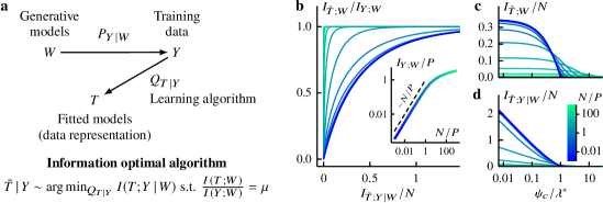
1.2 Information optimal algorithm
The data generating process above results in training data and true parameters that are Gaussian correlated (under the fixed design setting). In this case the IB optimization—minimizing residual information while maximizing relevant information —admits an exact solution [36], characterized by the eigenmodes of the normalized regression matrix,
| (5) |
where denotes the scaled noise-to-signal ratio. The relevant and residual informations of an optimal representation read [36]
| (6) | ||||
| (7) |
where denote the eigenvalues of and parametrizes the IB trade-off222The arguments of the logarithms in Eqs (6-7) are always nonnegative since the data processing inequality means that the IB problem is well-defined only for , and the eigenvalues of a normalized regression matrix always range from zero to one [36]. [see Eq (1)]. In our setting it is convenient to recast the summations above as integrals (see Appendix A for derivation),
| (8) | ||||
| (9) |
where and denote the empirical covariance and its cumulative spectral distribution, respectively.333Note that the eigenvalues of and are identical except for the number of zero modes. In addition we introduce the parameter which controls the number and the weights of eigenmodes used in constructing the optimal representation . In the limit , the residual information diverges logarithmically (Fig 1d) and the relevant information converges to the available relevant information in the data (Fig 1c),
| (10) |
Increasing from zero decreases both residual and relevant informations, tracing out the optimal frontier until the lower spectral cutoff reaches the upper spectral edge at which both informations vanish (Fig 1b) and beyond which no informative solution exists [36, 37, 38].
1.3 Information efficiency
The exact characterization of the IB frontier provides a useful benchmark for information-theoretic analyses of learning algorithms, not least because it allows a precise definition of information efficiency. That is, we can now ask how many more residual bits a given algorithm needs to encode, compared to the IB optimal algorithm, in order to achieve the same level of relevant information. Here we define the information efficiency as the ratio between the residual bits encoded in the outputs of the IB optimal algorithm and the algorithm of interest— and , respectively—at some fixed relevance level , i.e.,
| (11) |
Since the optimal representation minimizes residual bits at fixed (Fig 1a), the information efficiency ranges from zero to one, . In addition we have , resulting from the data processing inequality for the Markov constraint (see, e.g., Ref [39]).
2 Gibbs-posterior least squares regression
We consider one of the best-known learning algorithms: least squares linear regression. Not only is this algorithm widely used in practice, it has also proved a particularly well-suited setting for analyzing learning in the overparametrized regime [40, 41, 42, 43, 44, 45, 46, 47]. Indeed it exhibits some of the most intriguing features of overparametrized learning, including benign overfitting and double descent which describe the surprisingly good generalization performance of overparametrized models and its nonmonotonic dependence on model complexity and sample size [48, 42, 31].
Inferring a model from data generally requires an assumption on a class of models, which defines the hypothesis space, as well as a learning algorithm, which outputs a hypothesis according to some criteria that rank how well each hypothesis explains the data. Linear regression restricts the model class to a linear map, parametrized by , between an input and a predicted response ,
| (12) |
Minimizing the mean squared error yields a closed form solution for the estimated regressor, . However, this requires to be invertible and thus does not work in the overparametrized regime in which the sample covariance is not full rank and infinitely many models have vanishing mean squared error.
There are several approaches to break this degeneracy but perhaps the simplest and most studied is the ridge regularization which adds to the mean squared error the preference for model parameters with small norm, resulting in the regularized loss function
| (13) |
where controls the regularization strength. Minimizing this loss function leads to a unique solution even when .
Gibbs posterior—While ridge regression works in the overparametrized regime, it is a deterministic algorithm which does not readily lend itself to information-theoretic analyses because the mutual information between two deterministically related continuous random variables diverges. Instead we consider the Gibbs posterior (or Gibbs algorithm) which becomes a Gaussian channel when defined with the ridge regularized loss in Eq (13),
| (14) |
Here denotes the inverse temperature. In the zero temperature limit , this algorithm returns the usual ridge regression estimate (the mean of the above normal distribution) with probability approaching one. Whilst randomized ridge regression needs not take the form above, Gibbs posteriors are attractive, not least because they naturally emerge, for example, from information-regularized risk minimization [5] (see also Ref [27] for a recent discussion).
Markov constraint—The generative model , true parameter distribution and learning algorithm [Eqs (3-4) & (14)] completely describe the relationship between all random variables of interest through the Markov factorization of their joint distribution (Fig 1a),
| (15) |
Note that and in the fixed design setting (see Sec 1.1).
3 Information content of Gibbs regression
We now turn to the relevant and residual informations of the models that result from the Gibbs regression algorithm [Eq (14)]. Since all distributions appearing on the rhs of Eq (15) are Gaussian, the relevant and residual informations are given by
| (16) |
Here we use the fact that due to the Markov constraint [Eq (15)]. The covariance is defined by the learning algorithm in Eq (14). To obtain and , we marginalize out and in order from [Eqs (3-4) & (14-15)] and obtain
| (17) | ||||
| (18) |
Substituting the covariance matrices above into Eq (16) yields (see Appendix B for derivation)
| (19) | ||||
| (20) |
The integration domains are restricted to positive real numbers since the eigenvalues of a covariance matrix are non-negative and the integrands vanish at .
In the zero temperature limit , the residual information diverges (as expected from a deterministic algorithm [23, 24]; see also Fig 2c) whereas the relevant information approaches the mutual information between the data and the true parameter ,
| (21) |
Relevant and residual informations decrease with until they vanish as at which Gibbs posteriors become completely random (Fig 2a-c).

3.1 Zero temperature limit
At first sight it appears that our analyses are not applicable in the high-information limit since the residual information diverges for both the optimal algorithm and Gibbs regression (see Figs 1d & 2c). However the rates of divergence differ. Here we use this difference to characterize the efficiency of Gibbs regression in the zero temperature limit .
We first analyze the limiting behaviors of relevant information. From Eq (10), we see that the relevant information ratio of the IB solution approaches one at . Perturbing in Eq (8) away from zero results in a linear correction to the relevant information,
| (22) |
Keeping only the leading correction and recalling that [Eq (11)], we obtain
| (23) |
Similarly expanding the relevant information of Gibbs regression [Eq (19)] around yields
| (24) |
As a result, the correspondence between the low-temperature and high-information limits reads
| (25) |
We turn to the residual bits. Expanding Eq (9) around and Eq (20) around leads to
| (26) | ||||
| (27) |
From Eqs (23) & (25), we see that the residual informations above have the same logarithmic singularity, , at . Therefore their difference remains finite even as . Combining Eqs (23) & (25-27) and recalling our definition of information efficiency [Eq (11)] gives
| (28) |
Note that Jensen’s inequality guarantees that the terms in the parentheses sum to a non-negative value.
4 High dimensional limit
To place our results in the context of high dimensional learning, we specialize to the thermodynamic limit in which sample size and input dimension tend to infinity at a fixed ratio—that is, at . While it is easy to grow the dimension of the true parameter (Sec 1.1), we have so far not specified how the design matrix , and thus the training data , should scale in this limit.
To this end, we consider a setting in which the design matrix is generated from where is a matrix with iid entries drawn from a distribution with zero mean and unit variance, and is a covariance matrix.444This prescription includes the case where input vectors are drawn iid from for . If admits a limiting spectral density as , then the empirical spectral distribution becomes deterministic [49, 50].
To aid interpretation of our results, we frame all of the following discussions from the perspective that the input dimension is held fixed and a change in measurement density results only from a change in sample size .
4.1 Isotropic covariates
For , the empirical spectral distribution converges to to the standard Marchenko-Pastur law [49]
| (29) |
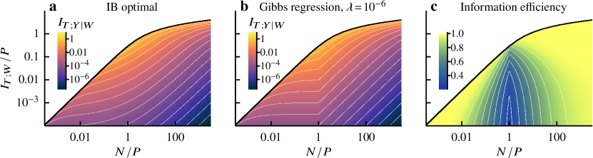
Optimal algorithm—In Fig 1b, the IB optimal frontiers illustrate the fundamental trade-off; optimal algorithms cannot encode fewer residual bits without becoming less relevant. Figure 1c-d shows that encoded relevant and residual bits go down as increases and fewer eigenmodes contribute to the IB optimal representation [Eqs (8-9)]. However relevant and residual informations exhibit different behaviors at high information; as , relevant information plateaus whereas residual information diverges logarithmically [see also Eq (26)].
Gibbs regression—Figure 2a depicts the information content of Gibbs regression at different regularization strengths [Eqs (19-20)] and illustrates the fundamental trade-off, similarly to the IB frontier (dotted) but at a lower relevance level. Here the information curves are parametrized by the inverse temperature which controls the algorithmic stochasticity; Gibbs posteriors become deterministic as and completely random at [Eq (14)]. In Fig 2b-c, we see that Gibbs regression encodes fewer relevant and residual bits as temperature goes up. Decreasing Gibbs temperature results in an increase in encoded information. In the zero-temperature limit, the relevant bits saturate while the residual bits grow logarithmically (cf. Fig 1c-d; see Sec 3.1 for a detailed analysis of this limit). The amount of encoded information depends also on the regularization strength . Figure 2b-c shows that, at a fixed temperature, an increase in leads to less information extracted. However this does not necessarily mean that a larger hurts information efficiency. Indeed a lower temperature can compensate for the decrease in information. In Fig 2a, we see that the information curves can be closer to the optimal frontier as increases. In general the maximum efficiency occurs at an intermediate regularization strength that depends on data structure and measurement density (see also Sec 4.2).
Efficiency—Figure 2d displays the information efficiency of Gibbs regression at different relevant information levels (see Sec 1.3). We see that the efficiency approaches optimality () in the limits and . Away from these limits, Gibbs regression requires more residual bits than the optimal algorithm to achieve the same level of relevance with an efficiency minimum around . We also see that the efficiency of Gibbs regression decreases with relevance level (see also Supplementary Figure in Appendix D).
Extensivity—Learning is qualitatively different in the over- and underparametrized regimes. In Fig 2e we see that both optimal algorithms and Gibbs regression exhibit nonmonotonic dependence on sample size. In the overparametrized regime , the residual information is extensive in sample size, i.e., it grows linearly with . This scaling behavior mirrors that of the relevant bits in the data (Fig 1b inset). But unlike the available relevant bits which continue to grow in the data-abundant regime, albeit sublinearly—the encoded residual bits decrease with sample size in this limit (see also Supplementary Figure in Appendix D). The resulting maximum is an information-theoretic analog of double descent—the decrease in overfitting level (test error) as the number of parameters exceeds sample size (decreasing ) [48, 31].
Redundancy—Indeed we could have anticipated the extensive behavior of the residual bits in the overparametrized regime (Fig 2e). In this limit, the extensivity of available relevant bits implies that the data encode relevant information with no redundancy. In other words, the relevant bits in one observation do not overlap with that in another. As a result, the dominant learning strategy is to treat each sample separately and extract the same amount of information from each of them, thus resulting in extensive residual information. In the data-abundant regime, on the other hand, the coding of relevant bits in the data becomes increasingly redundant (Fig 1b inset). Learning algorithms exploit this redundancy to better distinguish signals from noise, thereby encoding fewer residual bits.
4.2 Anisotropic covariates
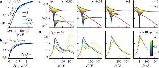
To explore the effects of anisotropy, we consider a two-scale model in which the population spectral distribution is an equal mixture of two point masses at and . We normalize the trace of the population covariance such that the signal variance, and thus the signal-to-noise ratio, does not depend on —i.e., we set such that . As a result the anisotropy in our two-scale model is parametrized completely by the eigenvalue ratio .
Unlike the isotropic case, the limiting empirical spectral distribution does not admit a closed form expression. We obtain by solving the Silverstein equation and inverting the resulting Stieltjes transform [51] (see Appendix C). Figure 3c depicts the spectral density at various anisotropy ratios and measurement densities. At high measurement densities , anisotropy splits the continuum part of the spectrum into two bands, corresponding to the two modes of the population covariance. These bands broaden as decreases and eventually merge into one in the overparametrized limit.
Available information—In Fig 3a, we see that anisotropy decreases the relevant information in the data, but does not affect its qualitative behaviors: the available relevant bits are extensive in the overparametrized regime and subextensive in the data-abundant regime. Although fewer relevant bits are available, learning needs not be less information efficient. Indeed the IB frontiers in Fig 3b illustrate that it takes fewer residual bits in the anisotropic case to reach the same level of relevance as in the isotropic case. This behavior is also apparent in Fig 3d (dotted) as we increase anisotropy levels (from right to left panels).
Anisotropy effects—Anisotropy affects optimal algorithms via the different scales in the population covariance. The signals along high-variance (easy) directions are stronger and, as a result, the coding of relevant bits in these directions becomes subextensive and redundant around (the proportion of easy directions) instead of at one (Fig 3a). This earlier onset of redundancy allows for more effective signal-noise discrimination in the anisotropic case (Fig 3b & d). In the data-abundant limit, however, low-variance (hard) directions become important as learning algorithms already encode most of the relevant bits along the easy directions. Indeed the hard directions are harder for more anisotropic inputs and thus the required residual bits increase with anisotropy in the limit (Fig 3d).
Triple descent—Perhaps the most striking effect of anisotropy is the emergence of an information-theoretic analog of (sample-wise) multiple descent, which describes disjoint regions where more data makes overfitting worse (larger test error) [32, 52]. In Fig 3d, we see that an additional residual information maximum emerges at large . This behavior is a consequence of the separation of scales. The first maximum at originates from easy directions and the other maximum at higher from hard directions. In fact the IB cutoff in Fig 3c demonstrates that the residual information maxima roughly coincide with the inclusion of all high-variance modes around and low-variance modes at higher .555Note that Fig 3c does not show the zero modes which are present at . The fact that the spectral continuum appears to be above the IB cutoff at small does not mean all eigenmodes are used in the IB solution. In addition we note that for optimal algorithms the first maximum shifts to a lower as the anisotropy level increases. This observation is consistent with the fact that the onset of redundancy of relevant bits in the data occurs at smaller in the anisotropic case (Fig 3a).
Gibbs regression—Anisotropy makes Gibbs regression depend more strongly on regularization strengths, see Fig 3. In particular the information efficiency decreases with near the first residual information minimum around but this dependence reverses near the second maximum and at larger . This behavior is expected. Inductive bias from strong regularization helps prevent noise from poisoning the models at small . But when the data become abundant, regularization is unnecessary.
5 Conclusion & Outlook
We use the information bottleneck theory to analyze linear regression problems and illustrate the fundamental trade-off between relevant bits, which are informative of the unknown generative processes, and residual bits, which measure overfitting. We derive the information content of optimal algorithms and Gibbs posterior regression, thus enabling a quantitative investigation of information efficiency. In addition our analytical results on the zero temperature limit of the Gibbs posterior offer a glimpse of a connection between information efficiency and optimally tuned ridge regression. Finally, using results from random matrix theory, we reveal the information complexity of learning a linear map in high dimensions and unveil an information-theoretic analog of multiple descent phenomena. Since residual information is an upper bound on the generalization gap [4, 5], we believe that this information nonmonotonicity could be connected to the original double descent phenomena. But it remains to be seen how deep this connection is.
Our work paves the way for a number of different avenues for future research. While we only focus on isotropic regularization here, it would be interesting to understand how structured regularization affects information extraction. Information-efficiency analyses of different algorithms, such as Bayesian regression, and other classes of learning problems, e.g., classification and density estimation, are also in order. An investigation of information efficiency based on other -divergence could lead to new insights into generalization. In particular an exact relationship exists between residual Jeffreys information and generalization error of Gibbs posteriors [27]. Finally exploring how coding redundancy in training data quantitatively affects learning phenomena in general would make for an exciting research direction (see, e.g., Refs [17, 19]).
Acknowledgments and Disclosure of Funding
This work was supported in part by the National Institutes of Health BRAIN initiative (R01EB026943), the National Science Foundation, through the Center for the Physics of Biological Function (PHY-1734030), the Simons Foundation and the Sloan Foundation.
References
References
- Belkin et al. [2018] M. Belkin, D. J. Hsu, and P. Mitra, Overfitting or perfect fitting? Risk bounds for classification and regression rules that interpolate, in Advances in Neural Information Processing Systems, Vol. 31, edited by S. Bengio, H. Wallach, H. Larochelle, K. Grauman, N. Cesa-Bianchi, and R. Garnett (Curran Associates, Inc., 2018).
- Belkin et al. [2019a] M. Belkin, A. Rakhlin, and A. B. Tsybakov, Does data interpolation contradict statistical optimality?, in Proceedings of the Twenty-Second International Conference on Artificial Intelligence and Statistics, Proceedings of Machine Learning Research, Vol. 89, edited by K. Chaudhuri and M. Sugiyama (PMLR, 2019) pp. 1611–1619.
- Tishby et al. [1999] N. Tishby, F. C. N. Pereira, and W. Bialek, The information bottleneck method, in 37th Allerton Conference on Communication, Control and Computing, edited by B. Hajek and R. S. Sreenivas (University of Illinois, 1999) pp. 368–377.
- Russo and Zou [2016] D. Russo and J. Zou, Controlling Bias in Adaptive Data Analysis Using Information Theory, in Proceedings of the 19th International Conference on Artificial Intelligence and Statistics, Vol. 51, edited by A. Gretton and C. C. Robert (PMLR, 2016) pp. 1232–1240.
- Xu and Raginsky [2017] A. Xu and M. Raginsky, Information-theoretic analysis of generalization capability of learning algorithms, in Advances in Neural Information Processing Systems, Vol. 30, edited by I. Guyon, U. V. Luxburg, S. Bengio, H. Wallach, R. Fergus, S. Vishwanathan, and R. Garnett (Curran Associates, Inc., 2017).
- Palmer et al. [2015] S. E. Palmer, O. Marre, M. J. Berry, and W. Bialek, Predictive information in a sensory population, Proceedings of the National Academy of Sciences 112, 6908 (2015).
- Wang et al. [2021] S. Wang, I. Segev, A. Borst, and S. Palmer, Maximally efficient prediction in the early fly visual system may support evasive flight maneuvers, PLOS Computational Biology 17, e1008965 (2021).
- Bauer et al. [2021] M. Bauer, M. D. Petkova, T. Gregor, E. F. Wieschaus, and W. Bialek, Trading bits in the readout from a genetic network, Proceedings of the National Academy of Sciences 118, e2109011118 (2021).
- Still et al. [2012] S. Still, D. A. Sivak, A. J. Bell, and G. E. Crooks, Thermodynamics of Prediction, Physical Review Letters 109, 120604 (2012).
- Gordon et al. [2021] A. Gordon, A. Banerjee, M. Koch-Janusz, and Z. Ringel, Relevance in the Renormalization Group and in Information Theory, Physical Review Letters 126, 240601 (2021).
- Kline and Palmer [2022] A. G. Kline and S. E. Palmer, Gaussian information bottleneck and the non-perturbative renormalization group, New Journal of Physics 24, 033007 (2022).
- Strouse and Schwab [2019] D. Strouse and D. J. Schwab, The Information Bottleneck and Geometric Clustering, Neural Computation 31, 596 (2019).
- Alemi et al. [2017] A. A. Alemi, I. Fischer, J. V. Dillon, and K. Murphy, Deep Variational Information Bottleneck, in International Conference on Learning Representations (2017).
- Achille and Soatto [2018] A. Achille and S. Soatto, Information Dropout: Learning Optimal Representations Through Noisy Computation, IEEE Transactions on Pattern Analysis and Machine Intelligence 40, 2897 (2018).
- Achille and Soatto [2018] A. Achille and S. Soatto, Emergence of Invariance and Disentanglement in Deep Representations, Journal of Machine Learning Research 19, 1 (2018).
- Goyal et al. [2019] A. Goyal, R. Islam, D. Strouse, Z. Ahmed, H. Larochelle, M. Botvinick, S. Levine, and Y. Bengio, Transfer and Exploration via the Information Bottleneck, in International Conference on Learning Representations (2019).
- Bialek et al. [2001] W. Bialek, I. Nemenman, and N. Tishby, Predictability, Complexity, and Learning, Neural Computation 13, 2409 (2001).
- Shamir et al. [2010] O. Shamir, S. Sabato, and N. Tishby, Learning and generalization with the information bottleneck, Theoretical Computer Science 411, 2696 (2010), Algorithmic Learning Theory (ALT 2008).
- Bialek et al. [2020] W. Bialek, S. E. Palmer, and D. J. Schwab, What makes it possible to learn probability distributions in the natural world? (2020).
- Alabdulmohsin [2017] I. Alabdulmohsin, An Information-Theoretic Route from Generalization in Expectation to Generalization in Probability, in Proceedings of the 20th International Conference on Artificial Intelligence and Statistics, Proceedings of Machine Learning Research, Vol. 54, edited by A. Singh and J. Zhu (PMLR, 2017) pp. 92–100.
- Nachum and Yehudayoff [2019] I. Nachum and A. Yehudayoff, Average-Case Information Complexity of Learning, in Proceedings of the 30th International Conference on Algorithmic Learning Theory, Proceedings of Machine Learning Research, Vol. 98, edited by A. Garivier and S. Kale (PMLR, 2019) pp. 633–646.
- Negrea et al. [2019] J. Negrea, M. Haghifam, G. K. Dziugaite, A. Khisti, and D. M. Roy, Information-Theoretic Generalization Bounds for SGLD via Data-Dependent Estimates, in Advances in Neural Information Processing Systems, Vol. 32, edited by H. Wallach, H. Larochelle, A. Beygelzimer, F. d'Alché-Buc, E. Fox, and R. Garnett (Curran Associates, Inc., 2019).
- Bu et al. [2020] Y. Bu, S. Zou, and V. V. Veeravalli, Tightening Mutual Information-Based Bounds on Generalization Error, IEEE Journal on Selected Areas in Information Theory 1, 121 (2020).
- Steinke and Zakynthinou [2020] T. Steinke and L. Zakynthinou, Reasoning About Generalization via Conditional Mutual Information, in Proceedings of Thirty Third Conference on Learning Theory, Proceedings of Machine Learning Research, Vol. 125, edited by J. Abernethy and S. Agarwal (PMLR, 2020) pp. 3437–3452.
- Haghifam et al. [2020] M. Haghifam, J. Negrea, A. Khisti, D. M. Roy, and G. K. Dziugaite, Sharpened Generalization Bounds based on Conditional Mutual Information and an Application to Noisy, Iterative Algorithms, in Advances in Neural Information Processing Systems, Vol. 33, edited by H. Larochelle, M. Ranzato, R. Hadsell, M. Balcan, and H. Lin (Curran Associates, Inc., 2020) pp. 9925–9935.
- Neu et al. [2021] G. Neu, G. K. Dziugaite, M. Haghifam, and D. M. Roy, Information-Theoretic Generalization Bounds for Stochastic Gradient Descent, in Proceedings of Thirty Fourth Conference on Learning Theory, Proceedings of Machine Learning Research, Vol. 134, edited by M. Belkin and S. Kpotufe (PMLR, 2021) pp. 3526–3545.
- Aminian et al. [2021] G. Aminian, Y. Bu, L. Toni, M. Rodrigues, and G. Wornell, An Exact Characterization of the Generalization Error for the Gibbs Algorithm, in Advances in Neural Information Processing Systems, Vol. 34, edited by M. Ranzato, A. Beygelzimer, Y. Dauphin, P. Liang, and J. W. Vaughan (Curran Associates, Inc., 2021) pp. 8106–8118.
- Chen et al. [2021a] Q. Chen, C. Shui, and M. Marchand, Generalization Bounds For Meta-Learning: An Information-Theoretic Analysis, in Advances in Neural Information Processing Systems, Vol. 34, edited by M. Ranzato, A. Beygelzimer, Y. Dauphin, P. Liang, and J. W. Vaughan (Curran Associates, Inc., 2021) pp. 25878–25890.
- Chalk et al. [2016] M. Chalk, O. Marre, and G. Tkacik, Relevant sparse codes with variational information bottleneck, in Advances in Neural Information Processing Systems, Vol. 29, edited by D. D. Lee, M. Sugiyama, U. V. Luxburg, I. Guyon, and R. Garnett (Curran Associates, Inc., 2016) pp. 1957–1965.
- Poole et al. [2019] B. Poole, S. Ozair, A. Van Den Oord, A. Alemi, and G. Tucker, On Variational Bounds of Mutual Information, in Proceedings of the 36th International Conference on Machine Learning, Proceedings of Machine Learning Research, Vol. 97, edited by K. Chaudhuri and R. Salakhutdinov (PMLR, 2019) pp. 5171–5180.
- Nakkiran et al. [2020] P. Nakkiran, G. Kaplun, Y. Bansal, T. Yang, B. Barak, and I. Sutskever, Deep Double Descent: Where Bigger Models and More Data Hurt, in International Conference on Learning Representations (2020).
- d'Ascoli et al. [2020] S. d'Ascoli, L. Sagun, and G. Biroli, Triple descent and the two kinds of overfitting: where & why do they appear?, in Advances in Neural Information Processing Systems, Vol. 33, edited by H. Larochelle, M. Ranzato, R. Hadsell, M. Balcan, and H. Lin (Curran Associates, Inc., 2020) pp. 3058–3069.
- Hastie et al. [2009] T. Hastie, R. Tibshirani, and J. Friedman, The Elements of Statistical Learning, 2nd ed. (Springer, 2009).
- Sheng and Dobriban [2020] Y. Sheng and E. Dobriban, One-shot Distributed Ridge Regression in High Dimensions, in Proceedings of the 37th International Conference on Machine Learning, Proceedings of Machine Learning Research, Vol. 119, edited by H. D. III and A. Singh (PMLR, 2020) pp. 8763–8772.
- Liu and Dobriban [2020] S. Liu and E. Dobriban, Ridge Regression: Structure, Cross-Validation, and Sketching, in International Conference on Learning Representations (2020).
- Chechik et al. [2005] G. Chechik, A. Globerson, N. Tishby, and Y. Weiss, Information bottleneck for Gaussian variables, Journal of Machine Learning Research 6, 165 (2005).
- Wu and Fischer [2020] T. Wu and I. Fischer, Phase Transitions for the Information Bottleneck in Representation Learning, in International Conference on Learning Representations (2020).
- Ngampruetikorn and Schwab [2021] V. Ngampruetikorn and D. J. Schwab, Perturbation Theory for the Information Bottleneck, in Advances in Neural Information Processing Systems, Vol. 34, edited by M. Ranzato, A. Beygelzimer, Y. Dauphin, P. Liang, and J. W. Vaughan (Curran Associates, Inc., 2021) pp. 21008–21018.
- Cover and Thomas [2006] T. M. Cover and J. A. Thomas, Elements of Information Theory, 2nd ed. (Wiley-Interscience, 2006).
- Dobriban and Wager [2018] E. Dobriban and S. Wager, High-dimensional asymptotics of prediction: Ridge regression and classification, The Annals of Statistics 46, 247 (2018).
- Hastie et al. [2022] T. Hastie, A. Montanari, S. Rosset, and R. J. Tibshirani, Surprises in high-dimensional ridgeless least squares interpolation, The Annals of Statistics 50, 949 (2022).
- Bartlett et al. [2020] P. L. Bartlett, P. M. Long, G. Lugosi, and A. Tsigler, Benign overfitting in linear regression, Proceedings of the National Academy of Sciences 117, 30063 (2020).
- Emami et al. [2020] M. Emami, M. Sahraee-Ardakan, P. Pandit, S. Rangan, and A. Fletcher, Generalization Error of Generalized Linear Models in High Dimensions, in Proceedings of the 37th International Conference on Machine Learning, Proceedings of Machine Learning Research, Vol. 119, edited by H. D. III and A. Singh (PMLR, 2020) pp. 2892–2901.
- Li et al. [2020] Z. Li, C. Xie, and Q. Wang, Provable More Data Hurt in High Dimensional Least Squares Estimator (2020).
- Wu and Xu [2020] D. Wu and J. Xu, On the Optimal Weighted Regularization in Overparameterized Linear Regression, in Advances in Neural Information Processing Systems, Vol. 33, edited by H. Larochelle, M. Ranzato, R. Hadsell, M. Balcan, and H. Lin (Curran Associates, Inc., 2020) pp. 10112–10123.
- Mel and Ganguli [2021] G. Mel and S. Ganguli, A theory of high dimensional regression with arbitrary correlations between input features and target functions: sample complexity, multiple descent curves and a hierarchy of phase transitions, in Proceedings of the 38th International Conference on Machine Learning, Proceedings of Machine Learning Research, Vol. 139, edited by M. Meila and T. Zhang (PMLR, 2021) pp. 7578–7587.
- Richards et al. [2021] D. Richards, J. Mourtada, and L. Rosasco, Asymptotics of Ridge(less) Regression under General Source Condition, in Proceedings of The 24th International Conference on Artificial Intelligence and Statistics, Proceedings of Machine Learning Research, Vol. 130, edited by A. Banerjee and K. Fukumizu (PMLR, 2021) pp. 3889–3897.
- Belkin et al. [2019b] M. Belkin, D. Hsu, S. Ma, and S. Mandal, Reconciling modern machine-learning practice and the classical bias-variance trade-off, Proceedings of the National Academy of Sciences 116, 15849 (2019b).
- Marčenko and Pastur [1967] V. A. Marčenko and L. A. Pastur, Distribution of eigenvalues for some sets of random matrices, Mathematics of the USSR–Sbornik 1, 457 (1967).
- Silverstein [1995] J. Silverstein, Strong Convergence of the Empirical Distribution of Eigenvalues of Large Dimensional Random Matrices, Journal of Multivariate Analysis 55, 331 (1995).
- Silverstein and Choi [1995] J. Silverstein and S. Choi, Analysis of the Limiting Spectral Distribution of Large Dimensional Random Matrices, Journal of Multivariate Analysis 54, 295 (1995).
- Chen et al. [2021b] L. Chen, Y. Min, M. Belkin, and A. Karbasi, Multiple Descent: Design Your Own Generalization Curve, in Advances in Neural Information Processing Systems, Vol. 34, edited by M. Ranzato, A. Beygelzimer, Y. Dauphin, P. Liang, and J. W. Vaughan (Curran Associates, Inc., 2021) pp. 8898–8912.
Appendix A Information content of maximally efficient algorithms
Consider an IB problem where we are interested in an information efficient representation of that is predictive of (Fig 1a). When and are Gaussian correlated, the central object in constructing an IB solution is the normalized regression matrix ; in particular, its eigenvalues completely characterize the information content of the IB optimal representation via (see Ref [36] for a derivation)
| (30) | ||||
| (31) |
where is the dimension of and parametrizes the IB trade-off [Eq (1)].
Our work focuses on the following generative model for and (see Sec 1.1)
| (32) |
Marginalizing out yields
| (33) |
As a result, the normalized regression matrix reads
| (34) |
Substituting Eq (34) into Eqs (30-31) gives
| (35) | ||||
| (36) |
where denote the eigenvalues of . Since the eigenvalues of and the sample covariance are identical except for the zero modes which do not contribute to information, we can recast the above equations as
| (37) | ||||
| (38) |
where are the eigenvalues of and the summation limits change to , the number of eigenvalues of . Introducing the cumulative spectral distribution and replacing the summations with integrals results in
| (39) | ||||
| (40) |
We see that the contributions to the integrals come from the logarithms but only when they are positive. This condition can be recast into integration limits (note that and )
| (41) | ||||
| (42) |
Finally we define the lower cutoff and use the above limits to rewrite the expressions for relevant and residual informations,
| (43) | ||||
| (44) |
These equations are identical to Eqs (8-9) in the main text.
Appendix B Information content of Gibbs-posterior regression
To compute the information content of Gibbs regression [Eq (14)], we first recall that the mutual information between two Gaussian correlated variables, and , is given by
| (45) |
where is the covariance of , and of .
We now write down the relevant information, using the covariances and from Eqs (17-18),
| (46) | ||||
| (47) | ||||
| (48) | ||||
| (49) | ||||
| (50) | ||||
| (51) |
where . In the above, we use the identity which holds for any positive-definite Hermitian matrix , let denote the eigenvalues of the sample covariance and introduce , the cumulative distribution of eigenvalues. We also assume that and are finite and positive. Note that the integral is limited to positive real numbers because the eigenvalues of a covariance matrix is non-negative and the integrand vanishes for .
Appendix C Marchenko-Pastur law
Consider where is a matrix with iid entries drawn from a distribution with zero mean and unit variance, and is a covariance matrix. In addition we take the asymptotic limit , and . If the population spectral distribution converges to a limiting distribution, the spectral distribution of the sample covariance becomes deterministic [49]. The density, , is related to its Stieltjes transform via
| (56) |
We can obtain by solving the Silverstein equation for the companion Stieltjes transform [51],
| (57) |
and using the relation
| (58) |
Here denotes the upper half of the complex plane.
Appendix D Supplementary figure