Information Geometry for Maximum Diversity Distributions

This paper examines the application of information geometry to biodiversity measurement. Various indices, including the Simpson-Gini index, Hill numbers, and Rao’s quadratic entropy, have been developed and utilized to assess the ecological states of biological communities. In particular, Rao’s quadratic entropy has become a cornerstone of biodiversity research , which incorporates both species abundance and functional or genetic dissimilarity, see Rao (1982a, b). By combining species abundance with functional or genetic differences, Rao’s quadratic entropy offers a comprehensive tool for ecological and population genetics studies, enabling ecologists to measure and interpret diversity in ways that were not possible before. By combining species abundance with functional and genetic differences across large datasets, it provides insights into ecosystem stability, resilience, and conservation needs. As computational power and data accessibility continue to grow, Rao’s quadratic entropy will likely remain at the forefront of biodiversity assessments, driving advances in ecological understanding and environmental stewardship. Rao’s groundbreaking contributions in statistical theory and information geometry have had a profound influence on the development of diversity measures, see Rao (1945). His introduction of the Fisher-Rao information metric laid the foundation for viewing statistical models as geometric entities, an approach that has become instrumental in machine learning, ecological modeling, and data science, see Rao (1961, 1987).

We present a comprehensive review of diversity indices through the lens of information geometry. This approach highlights the deep interconnections between Rao’s information-theoretic measures and ecological resilience, revealing how the geometric properties of diversity measures can enhance our understanding of community structure. Specifically, we discuss the maximum diversity distributions under linear constraints, examining how ecological factors, such as resource limitations or habitat suitability, can be represented as geometric constraints on species distributions. We reduce the problem of finding the maximal distribution to a mathematical optimization characterized by the Karush-Kuhn-Tucker (KKT) conditions to find an optimal solution. We demonstrate that the maximum Hill-number distributions can be characterized using $q$-geodesics, which generalize the concept of geodesic paths in the simplex and provide insightful connections between statistical estimation and ecological interpretations. This approach extends Rao’s vision of information geometry, providing ecologists and conservationists with a robust method for identifying optimal diversity configurations in response to environmental constraints. In addition, we propose practical applications for this framework, emphasizing how Rao’s contributions to information geometry continue to shape and advance biodiversity research, guiding conservation strategies and promoting a deeper understanding of ecosystem dynamics. From this information-geometric viewpoint, we offer valuable insights into ecosystem stability and resilience. Our approach not only advances theoretical understanding but also has practical implications for biodiversity conservation and environmental management.

The paper is organized as follows: Section 2 builds a mathematical framework for diversity measures, in which we overview the standard indices of diversity such as the Gini-Simpson index, the Hill number and Rao’s quadratic entropy. In Section 3 we present an idea of maximum divergence distributions under a linear constraint focusing on the Hill numbers. The approach is extended to a case of multiple constraints. The ecological interpretation is explored from the practical point of view. Section 4 gives information-geometric understanding for the maximum divergence distributions in a simplex, or a space of categorical distributions. Notably, we associate a foliation, a partitioning into submanifolds, of the simplex with the maximum divergence distribution under linear constraints. This geometric structure provides deeper insight into the behavior of diversity measures within the simplex of categorical distributions. In Section 5 we discuss the maximum divergence distribution in comprehensive perspectives.

We provide an overview of common measures used to quantify the diversity of a community, cf. May (1975). Consider a community with $S$ species, where $p_{i}$ represents the relative abundance of species $i$. The set of all possible relative abundance vectors is represented by the $(S-1)$-dimensional simplex:

$$\Delta_{S-1}=\Big{\{}\mbox{\boldmath$p$}=(p_{1},\ldots,p_{S}):\sum_{i=1}^{S}p_{i}=1,\,p_{i}\geq 0\,(i=1,\ldots,S)\Big{\}}.$$

Henceforth, we will identify $\Delta_{S-1}$ with the set of all $S$-variate categorical distributions. The following measures of diversity, applied in various ecological contexts, enable various views of biodiversity, emphasizing different aspects from species evenness and dominance. The Gini-Simpson index is given by

$$D_{\text{GS}}({\mbox{\boldmath$p$}})=1-\sum_{i=1}^{S}p_{i}^{2}$$

for ${\mbox{\boldmath$p$}}=(p_{i})$ of $\Delta_{S-1}$, see Simpson (1949). The Gini-Simpson index represents the probability that two randomly selected individuals from a community belong to different species. This index is sensitive to species evenness and increases as species abundances become more evenly distributed. The Hill Numbers provide a general framework for diversity that is sensitive to the order $q$, which adjusts the emphasis on species richness versus evenness. The Hill number of order $q$ is defined as:

$\displaystyle{}^{q}\!D({\mbox{\boldmath$p$}})=\left(\sum_{i=1}^{S}p_{i}{}^{q}\!\right)^{\frac{1}{1-q}}$

(1)

where $q$ is a controlling parameter that determines the sensitivity of the index to species abundances, see Hill (1973). When $q=0$, ${}^{0}\!D({\mbox{\boldmath$p$}})=S$, which is simply species richness (the count of species). When $q$ goes to $1$, the measure becomes Boltzmann-Shannon entropy, with ${}^{q}\!D({\mbox{\boldmath$p$}})$ calculated as ${}^{1}\!D({\mbox{\boldmath$p$}})=\exp\left(H({\mbox{\boldmath$p$}})\right),$ where

$$H({\mbox{\boldmath$p$}})=-\sum_{i=1}^{S}p_{i}\log(p_{i}).$$

This form uses the exponential of Boltzmann-Shannon entropy $H({\mbox{\boldmath$p$}})$ to remain in the Hill framework. This quantifies the uncertainty in predicting the species of a randomly chosen individual. It is maximized when all species are equally abundant, indicating high diversity, and decreases as dominance by fewer species increases. When $q=2$, The measure reduces to the inverse Simpson index

$${}^{2}\!D({\mbox{\boldmath$p$}})=\left(\sum_{i=1}^{S}p_{i}^{2}\right)^{-1}$$

which gives greater weight to common species and is particularly useful for measuring dominance. Thus, the parameter $q$ adjusts the sensitivity of the Hill number to species abundances, with higher $q$-values emphasizing dominant species and lower values favoring rare species. The Berger-Parker index focuses on dominance by measuring the proportional abundance of the most abundant species

$$D_{\text{BP}}({\mbox{\boldmath$p$}})=\max(p_{i})$$

where $p_{i}$ is the relative abundance of each species. The Berger-Parker index is useful for identifying communities dominated by a single or few species, with higher values indicating lower diversity and higher dominance by certain species. Alternatively, the inverse Berger-Parker index $1/D_{\text{B}P}({\mbox{\boldmath$p$}})$ can be used as a diversity measure, where higher values indicate greater diversity. When the order of the Hill number goes to infinity, it goes the inverse Berger-Parker index. This is because

$$\lim_{q\rightarrow\infty}{}^{q}\!D({\mbox{\boldmath$p$}})=\lim_{q\rightarrow\infty}\left[\max(p_{i})\left\{\sum_{i=1}^{S}\left(\frac{p_{i}}{\max(p_{i})}\right)^{q}\right\}^{\frac{1}{q}}\right]^{\frac{q}{1-q}}$$

which is nothing but $1/D_{\text{B}P}({\mbox{\boldmath$p$}})$. Alternatively, as $q\rightarrow-\infty$, the Hill number converges to the inverse of the smallest relative abundance: $\lim_{q\rightarrow-\infty}{}^{q}\!D({\mbox{\boldmath$p$}})=1/\min_{i}(p_{i})$.

Rao’ s quadratic entropy is a measure of diversity that accounts not only for species abundance but also for the dissimilarity between species, such as functional or genetic differences, see Rao (1982a, b). It is defined as

$${\mathrm{Q}}({\mbox{\boldmath$p$}})=\sum_{i=1}^{S}\sum_{j=1}^{S}p_{i}p_{j}{W}_{ij},$$

where $\mbox{\boldmath$p$}=(p_{1},...,p_{S})$ represents the relative abundances, and $W_{ij}$ is a measure of dissimilarity between species $i$ and $j$ satisfying $W_{ii}=0$ and $W_{ij}\geq 0$. For example, the dissimilarity matrix is often derived from a distance matrix calculated using measures such as Gower’s distance, Manhattan distance, and others, see Botta-Dukát (2005); Southwood and Henderson (2009). Rao’ s quadratic entropy increases with both the abundance of different species and their functional or genetic differences.

When $W_{ij}=1$ for all $i\neq j$, Rao’s quadratic entropy reduces to a form of the Gini-Simpson index. This measure is particularly useful for quantifying functional diversity in ecosystems where species differ in ecological roles or genetic traits. The Hill number ${}^{q}\!D({\mbox{\boldmath$p$}})$ is a family of diversity indices parameterized by $q$, which controls the sensitivity of the measure to species abundances. Hill numbers are ‘effective’ numbers, meaning they give an intuitively meaningful measure of the effective number of species in a community by reflecting both species abundances and the emphasis on common versus rare species through the parameter $q$. Rao’s quadratic entropy, on the other hand, incorporates both species abundances and a dissimilarity matrix that quantifies pairwise similarities between species, allowing it to account for the phylogenetic or functional differences between them. Mathematically, it is defined as the expected dissimilarity between two randomly chosen individuals from a community. In essence, Rao’s entropy provides a diversity measure that is sensitive not only to species abundances but also to their similarity, making it valuable for communities where species may vary significantly in terms of genetic, functional, or ecological traits. To integrate these two concepts the Leinster-Cobbold index is proposed by

$${}^{q}\!D_{\mbox{\scriptsize\boldmath$Z$}}({\mbox{\boldmath$p$}})=\left(\sum_{i=1}^{S}p_{i}({\mbox{\boldmath$Z$}}{\mbox{\boldmath$p$}})_{i}^{q-1}\right)^{\frac{1}{1-q}}$$

where $Z$ is the similarity matrix with entries $Z_{ij}$ representing the similarity between species $i$ and $j$ satisfying $Z_{ii}=1$ and $0\leq Z_{ij}\leq 1$, see Leinster and Cobbold (2012). The term $(\mbox{\boldmath$Z$}\mbox{\boldmath$p$})_{i}=\sum_{j=1}^{S}Z_{ij}p_{j}$ is the average similarity of species $i$ to all species in the community, weighted their relative abundances. This retains the effective number interpretation of Hill numbers while incorporating a similarity matrix like Rao’s quadratic entropy. For a given community, they define a generalized diversity measure that combines both relative abundances and similarities among species. The sensitivity parameter $q$ of the Hill number framework is retained, controlling the emphasis on rare versus common species, and a similarity matrix $Z$ quantifies species resemblance. Leinster and Cobbold’s index ${}^{2}\!D_{\mbox{\scriptsize\boldmath$Z$}}({\mbox{\boldmath$p$}})$ with $q=2$ simplifies

$${}^{2}\!D_{\mbox{\scriptsize\boldmath$Z$}}(\mbox{\boldmath$p$})=\frac{1}{\mbox{\boldmath$p$}^{\top}\mbox{\boldmath$Z$}\mbox{\boldmath$p$}},$$

which, under some conditions, aligns with the inverse of Rao’s quadratic entropy when $\mbox{\boldmath$Z$}={\bf I}-\mbox{\boldmath$W$}$ (i.e., the similarity matrix is derived from the dissimilarity matrx). This makes it a direct similarity-sensitive generalization of the Gini-Simpson index. By varying $q$, one obtains a diversity profile that reflects different levels of sensitivity to rare and common species, while the similarity matrix $Z$ ensures that closely related species contribute less to the overall diversity measure. This connection allows both Hill numbers and Rao’s entropy to be seen as part of a single framework, with ${}^{q}\!D_{\mbox{\scriptsize\boldmath$Z$}}({\mbox{\boldmath$p$}})$ converging to the traditional Hill numbers when species are maximally distinct (i.e., the similarity matrix $Z$ is an identity matrix). In this unified measure, the flexibility of Hill numbers in emphasizing different aspects of species abundance combines with Rao’s consideration of species dissimilarity, providing a comprehensive and adaptable biodiversity measure that bridges the strengths of both approaches.

This section explores the mathematical foundations of maximizing biodiversity measures, focusing on Hill numbers, Rao’s quadratic entropy, and the Leinster-Cobbold index. We present optimization results under realistic ecological constraints, such as linear resource limits, and examine their implications for understanding community dynamics. By integrating these mathematical insights with ecological interpretations, we aim to provide a robust framework for evaluating and managing biodiversity in both theoretical and applied contexts.

Hill numbers ${}^{q}\!D({\mbox{\boldmath$p$}})$are interpreted as effective species counts, emphasizing their bounded nature and ensuring that the do not exceed the actual species count $S$, see Hill (1973); Jost (2006). Here, we confirm the maximum of the Hill numbers within a mathematical framework.

Extending this result, over a $(K-1)$-dimensional simplex $\Delta_{K-1}$ (i.e., considering only $K$ out of $S$ species), the Hill number ${}^{q}\!D({\mbox{\boldmath$p$}})$ attains its maximum value $K$ when $p$ is the uniform distribution over those $K$ species, with $p_{i}=\frac{1}{K}$ for the $K$ species and $p_{i}=0$ for the remaining $S-K$ species. In this way, the Hill number satisfies $1\leq{}^{q}\!D({\mbox{\boldmath$p$}})\leq S$. When ${}^{q}\!D({\mbox{\boldmath$p$}})=1$, the community is entirely dominated by a single species, indicating. Conversely, when ${}^{q}\!D({\mbox{\boldmath$p$}})=S$, the community has maximum diversity with species occurring in equal abundances. Therefore, the Hill number ${}^{q}\!D({\mbox{\boldmath$p$}})$ represents the effective number of species, providing a meaningful measure of diversity that accounts for both species richness and evenness. It is helpful to compare values of the Hill number across different ecosystems or treatments, considering both the index value and how close it is to its theoretical maximum for that number of species, see Chao (1987) for ecological perspectives.

However, in real ecosystems, perfect evenness is rare, and the maximizing may not always be ecologically desirable or feasible, see Colwell and Coddington (1994). Maximizing the Hill number might conflict with other ecological goals or constraints. To address this, we introduce a linear constraint on species distribution to reflect real-world ecological limits like resource availability, climate tolerance, and habitat capacity. We fix a linear constraint

$$\sum_{i=1}^{S}a_{i}p_{i}=C,$$

where $a_{i}$’s and $C$ are fixed constants. Here, without losing generality, we assume $a_{i}$ is positive. The constant $C$ reflects a fixed ecological limit, which lies within the range $a_{\rm min}\leq C\leq a_{\rm max}$ to ensure the existence for feasible $\mbox{\boldmath$p$}=(p_{i})$, where $a_{\min}=\min_{i}a_{i}$ and $a_{\max}=\max_{i}a_{i}$. In practice, the value of $C$ is often set as $C=\sum_{i=1}^{S}a_{i}\hat{\pi}_{i},$ where $\hat{\pi}_{i}$ represents an initial estimate of species proportions based on preliminary field data or other relevant ecological information. This approach anchors $C$ in observed or estimated ecological conditions, providing a realistic basis for the constraint on species distribution. This can represent ecological factors such as resource preference, habitat suitability, or species-specific traits. For instance, in a desert ecosystem, $a_{i}$ might represent drought tolerance in plants, favoring species with high $a_{i}$ values as they better adapt to dry conditions. The distribution can reflect species’ access to shared resources under competition. Species with high $a_{i}$ values may beat others in resource acquisition, resulting in larger $p_{i}$ values.

In this context, the linear constraint model is particularly relevant for habitats where specific resources are scarce and heavily contested. Such constraints shape community structures by influencing which species thrive, based on factors such as resource efficiency or adaptability to environmental conditions. For a general value of $q$ in the Hill number framework, the maximum Hill number distribution under a linear constraint is characterized by a power-law form of $q$ as follows.

We note that, if $q=1$, then the equilibrium is well-known as the maximum entropy distribution:

$$\hat{p}_{\theta i}=\frac{\exp(\theta a_{i})}{\sum_{j=1}^{S}\exp(\theta a_{j})}\quad(i=1,...,S),$$

in which the equilibrium distribution can be defined for any $C$ of the fully feasible interval $(a_{\min},a_{\max})$. This is referred to as a softmax function that is widely utilized in the field of Machine Learning. It also closely related to MaxEnt model that is important as a species distribution model, see Phillips et al. (2004).

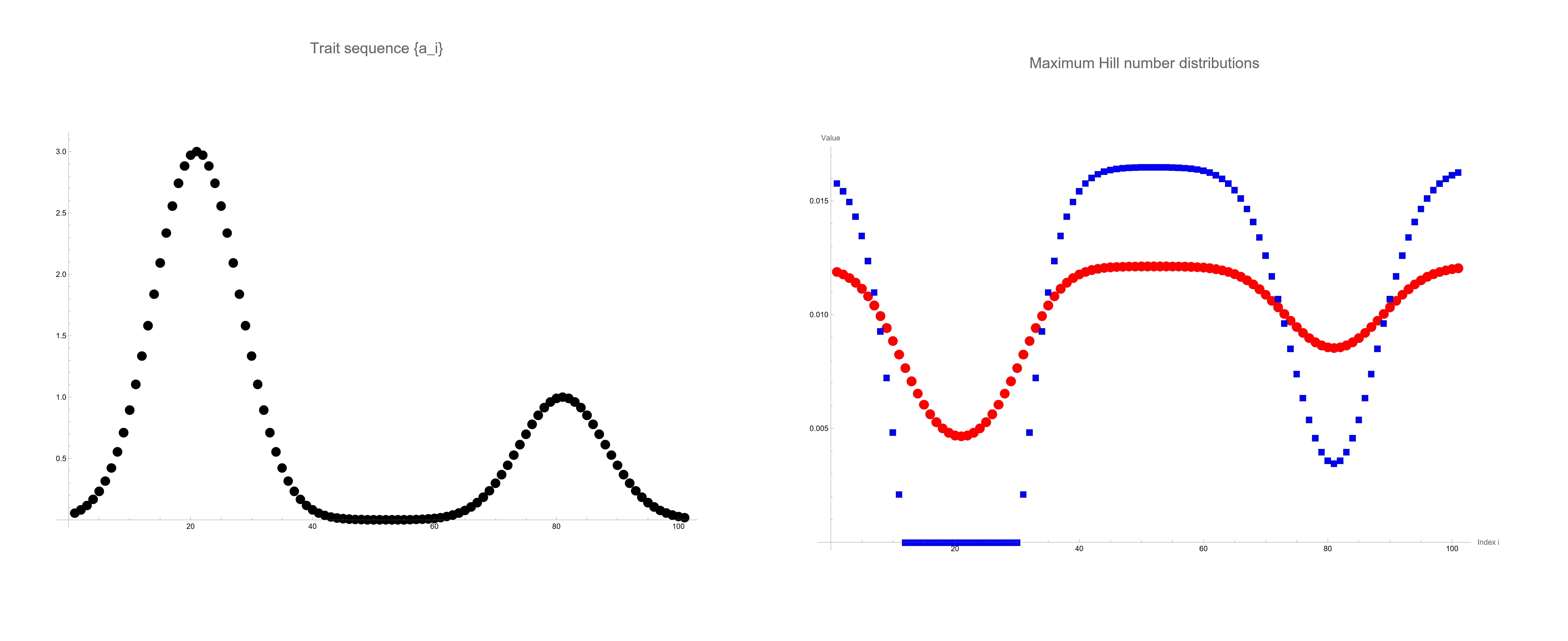
To illustrate the application of Proposition 2, we consider a community with $101$ species, where the trait $a_{i}$ for species $i$ is given by

$$a_{i}=3\exp\{-(i-20)^{2}/100\}+\exp\{-(i-80)^{2}/100\}\quad(i=1,...,101).$$

This trait distribution creates two peaks, representing species with higher ecological advantages. We compute the maximum ${}^{q}\!D$ distributions under this linear constraint $\sum_{i=1}^{101}a_{i}p_{i}=C$ with $C=0.2$ and $C=0.5$ for $q=2$ and $q=0.7$, respectively. The results are shown in Fig. 1. The left panel of Fig. 1displays the trait values $a_{i}$ against species $i$. The right panel shows the optimized species distribution for $q=2$ (squares) and $q=0.7$ (circles). For $q=2$, the distribution assigns zero probability to species with indices between $i=11$ and $i=30$, indicating that these species are excluded from the optimal distribution due to the emphasis on common species. For $q=0.7$, the distribution includes all species with non-zero probabilities, promoting evenness across the species. Indeed, for $q=0.7$, the Hill number is more sensitive to rare species, resulting in a more uniform distribution of probabilities among the species. We note that this numerical study can be conducted by solving only a one-parameter equation for $\theta$ to satisfy the linear constraint thanks to the result of Proposition 2. Thus, the optimization problem with 101 variables is drastically reduced to such a simplified one.

We discuss ecological meaning for $C_{\mbox{\scriptsize\boldmath$a$}}$, which represents a critical value in the linear constraint. If $C$ satisfy $C<C_{\mbox{\scriptsize\boldmath$a$}}$ for a case of $q<1$, then the optimal distribution becomes degenerate, meaning that it assigns zero probability to some species. This occurs because the resource constraint $C$ is too restrictive to allow for a distribution where all species have positive abundances. Ecologically, this reflects situations where only species with certain trait values $a_{i}$ can survive under the given constraints, leading to competitive exclusion and reduced diversity. Thus, the ecosystem cannot sustain all species at non-zero abundances without violating resource constraints. Fig. 2 gives a 3-D plot of the Hill number ${}^{q}\!D({\mbox{\boldmath$p$}})$ against $p$ of a $2$-dimensional simplex with $q=1$. In the surface, the curve $\{\hat{\mbox{\boldmath$p$}}_{\theta}\}_{\theta}$ has the centered point that attains the global maximum $3$ of ${}^{q}\!D({\mbox{\boldmath$p$}})$.

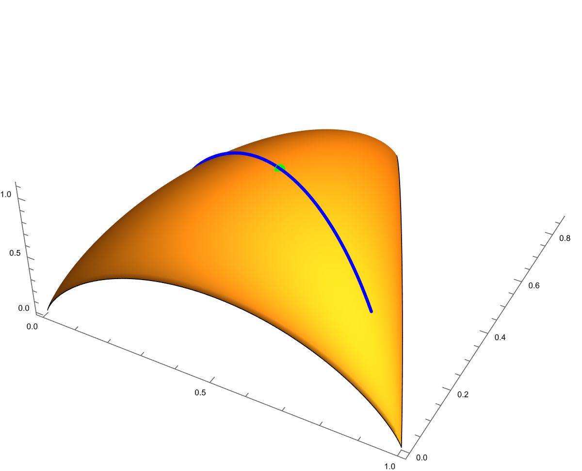
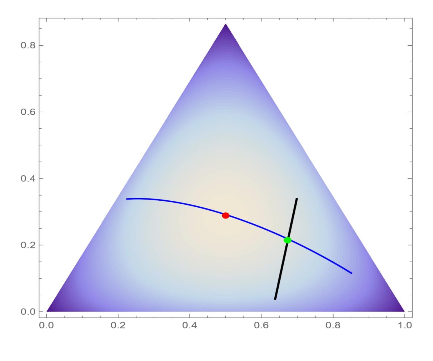
Fig. 3 gives a contour plot of the Hill number ${}^{q}\!D({\mbox{\boldmath$p$}})$ against $p$ of a $2$-dimensional simplex with $q=1$. In the simplex, the curve represents the model $\{{\mbox{\boldmath$p$}}_{\theta}\}_{\theta}$ intersects the line defined by the linear constrain at the point with the conditional maximum; the centered point attains the global maximum $3$ of ${}^{q}\!D({\mbox{\boldmath$p$}})$.

On the other hand, Rao’s quadratic entropy stands out for its ability to incorporate not only species abundance but also functional and genetic dissimilarities. Let us look into the distribution maximizing Rao’s quadratic entropy.

We discuss a case where entries of $\mbox{\boldmath$W$}^{-1}{\bf 1}$ have positive and negative signs. The optimal distribution would be in the boundary of $\Delta_{S-1}$, however any closed form is not solved here. For example, consider the following examples of a dissimilarity matrix:

$$\mbox{\boldmath$W$}_{1}=\begin{bmatrix}0&1&2&3\\ 1&0&3&2\\ 2&3&0&3\\ 3&2&2&0\end{bmatrix},\quad\mbox{\boldmath$W$}_{2}=\begin{bmatrix}0&1&2&3\\ 1&0&2&1\\ 2&2&0&1\\ 3&1&1&0\end{bmatrix}.$$

Then, we find $\mbox{\boldmath$W$}_{1}^{-1}{\bf 1}=(\frac{3}{23},\frac{3}{23},\frac{4}{23},\frac{4}{23})^{\top}$, which satisfies the assumption Proposition 3. The maximum of Rao’s entropy defined by $\mbox{\boldmath$W$}_{1}$ is $\frac{14}{23}$ at the optimal distribution $(\frac{3}{14},\frac{3}{14},\frac{2}{7},\frac{2}{7})^{\top}$. On the other hand, $\mbox{\boldmath$W$}_{2}^{-1}{\bf 1}=(-2,4,3,-3)^{\top}$, which violates the assumption Proposition 3. Indeed, the optimal distribution is given by $(\frac{1}{2},0,0,\frac{1}{2})^{\top}$ in the boundary, at which Roa’s entropy has a maximum $\frac{3}{2}$. These species with zero probabilities are effectively excluded from the ecosystem’s diversity under the entropy maximization principle, meaning they ”cannot survive” within the model’s framework.

If all species are equally dissimilar, then the global maximum distribution $\hat{p}_{0}^{(\rm Q)}$ equals the even distribution $e$. In effect, consider the case where ${\mbox{\boldmath$W$}}={\bf 1}{\bf 1}^{\top}-{\bf I}$, where $\bf I$ denotes the identity matrix. Then, ${\mbox{\boldmath$W$}}^{-1}=\frac{1}{S-1}{\bf 1}{\bf 1}^{\top}-{\bf I},$ and hence, $\hat{\mbox{\boldmath$p$}}_{0}^{\rm(Q)}$ equals the even distribution $e$. This is the same as the maximizer of ${}^{q}D({\mbox{\boldmath$p$}})$ noting that Rao’s quadratic entropy is reduced to the Gini-Simpson index. However, in most realistic scenarios, species differ in their functional or genetic traits, leading to variations in dissimilarities. Therefore, $\hat{\mbox{\boldmath$p$}}_{0}^{(\rm Q)}$ typically differs from $e$, giving higher probabilities to species more dissimilar to others. Next, consider another simple case where ${\mbox{\boldmath$W$}}_{\mbox{\scriptsize\boldmath$\pi$}}={\mbox{\boldmath$\pi$}}{\mbox{\boldmath$\pi$}}^{\top}-{\rm diag}({\mbox{\boldmath$\pi$}}^{2})$ for a fixed $\pi$ of $\Delta_{S-1}$, where $\rm diag$ denotes the diagonal matrix. Thus,

$${\mbox{\boldmath$W$}}_{\mbox{\scriptsize\boldmath$\pi$}}^{-1}=\frac{1}{S-1}{\mbox{\boldmath$\pi$}}^{-1}({\mbox{\boldmath$\pi$}}^{-1})^{\top}-{\rm diag}({\mbox{\boldmath$\pi$}}^{-2}),$$

and hence $({\mbox{\boldmath$W$}}_{\mbox{\scriptsize\boldmath$\pi$}}^{-1}{\bf 1})_{i}=\frac{{\bf 1}^{\top}\mbox{\scriptsize\boldmath$\pi$}^{-1}}{S-1}{\pi_{i}}^{-1}-{\pi_{i}}^{-2}$. This yields that, if $\pi_{i}>\frac{S-1}{{\bf 1}^{\top}\mbox{\scriptsize\boldmath$\pi$}^{-1}}$, then $({\mbox{\boldmath$W$}}_{\mbox{\scriptsize\boldmath$\pi$}}^{-1}{\bf 1})_{i}<0$, or the probability of species $i$ is a zero in the maximum distribution. Further, assume $\mbox{\boldmath$\pi$}=(\alpha\tilde{\bf 1},\beta\tilde{\bf 1})/m(\alpha+\beta)$, where $S=2m$ and $\tilde{\bf 1}$ is the one-copy vector of $m$ dimension. Then, a straightforward calculus yields that, if

$$\Big{|}\frac{\alpha}{\alpha+\beta}-\frac{1}{2}\Big{|}\leq\frac{1}{2(2m-1)},$$

then $\hat{\mbox{\boldmath$p$}}_{0}^{(\rm Q)}$ defined in (5) is in $\Delta_{S-1}$. This situation is quite near the case of $\alpha=\beta$, or the equally-dissimilar case $W$. In general, it is difficult to get a closed form of the maximum distribution without the assumption ${\mbox{\boldmath$W$}}^{-1}{\bf 1}>{\bf 0}$. However, we can use efficient algorithms to find numerically the maximizer, in which the optimization problem is reduced a a standard quadratic programming problem. Fast solvers like interior-point methods, active set methods, or alternating direction method of multipliers can handle this formulation. Tools such as quadprog in R and Python or specialized libraries like Gurobi or CVXPY provide robust implementations for high-dimensional problems. See Dostál (2009) for quadratic programming algorithms.

Next, consider a linear constraint: ${\mbox{\boldmath$a$}}^{\top}{\mbox{\boldmath$p$}}=C$, where ${\mbox{\boldmath$a$}}\geq\bf{0}$ and $C$ are fixed constants. Then, under the linear constraint, Similarly, we introduce the Lagrangian function:

$$\frac{1}{2}{\rm Q}({\mbox{\boldmath$p$}})+\mu\left({\mathbf{1}}^{\top}{\mbox{\boldmath$p$}}-1\right)+\lambda\left({\mbox{\boldmath$a$}}^{\top}{\mbox{\boldmath$p$}}-C\right).$$

The stationarity equation is given by ${\mbox{\boldmath$W$}}{\mbox{\boldmath$p$}}+\lambda{\mbox{\boldmath$a$}}+\mu{\mathbf{1}}={\bf 0},$ which yields the solution form:

$\displaystyle\hat{\mbox{\boldmath$p$}}_{\theta}^{({\rm Q})}=\frac{{\mbox{\boldmath$W$}}^{-1}({\bf 1}+\theta{\mbox{\boldmath$a$}})}{{\bf 1}^{\top}({\mbox{\boldmath$W$}}^{-1}({\bf 1}+\theta{\mbox{\boldmath$a$}}))}.$

(6)

Here $\theta$ is determined by the linear constraint, so that

$$\theta=\frac{(C{\bf 1}-\mbox{\boldmath$a$})^{\top}{\mbox{\boldmath$W$}}^{-1}{\bf 1}}{(C{\bf 1}-\mbox{\boldmath$a$})^{\top}{\mbox{\boldmath$W$}}^{-1}{\mbox{\boldmath$a$}}}.$$

If we assume ${\mbox{\boldmath$W$}}^{-1}({\bf 1}+\theta{\mbox{\boldmath$a$}})>0$, then $\hat{\mbox{\boldmath$p$}}_{\theta}^{({\rm Q})}$ is properly the distribution maximizing Rao’s entropy due to the discussion similar to the proof of Proposition 3.

Let us examine the maximum Leinster-Cobbold index distribution. This index is integrated the Hill number with Rao’s quadratic entropy, providing a unified framework for measuring biodiversity that accounts for both species abundances and similarities.. We can find the maximizing distribution by combining arguments in Propositions 2 and 3.

It is worthwhile to note that $\hat{\mbox{\boldmath$p$}}_{\rm LC}^{(q)}$ is independent of $q$, and is the same form as the maximum Rao’s entropy distribution $\hat{\mbox{\boldmath$p$}}_{0}^{\rm(Q)}$ defined in (5). The distribution maximizing under a linear constraint ${\mbox{\boldmath$a$}}^{\top}{\mbox{\boldmath$p$}}=C$ is given by

$\displaystyle\hat{\mbox{\boldmath$p$}}_{\theta}^{({\rm LC})}=\frac{{\mbox{\boldmath$Z$}}^{-1}\big{(}{\bf 1}+(q-1)\theta{\mbox{\boldmath$a$}}\big{)}^{\frac{1}{q-1}}}{{\bf 1}^{\top}{\mbox{\boldmath$Z$}}^{-1}\big{(}{\bf 1}+(q-1)\theta{\mbox{\boldmath$a$}}\big{)}^{\frac{1}{q-1}}},$

(8)

where $\theta$ is determined by $C$. We confirm that, if $q=2$, then $\hat{\mbox{\boldmath$p$}}_{\theta}^{({\rm LC})}$ is reduced to $\hat{\mbox{\boldmath$p$}}_{\theta}^{({\rm Q})}$ defined in (6) by a re-parameterized $\theta$; if ${\mbox{\boldmath$Z$}}={\bf I}$, then this is reduced to $\hat{\mbox{\boldmath$p$}}_{\theta}$ in (3). Thus, this effectively integrates both maximum distributions. Then, the stationarity condition is written by

$$q(\mbox{\boldmath$Zp$})^{q-1}+\lambda{\mbox{\boldmath$a$}}+\mu{\mathbf{1}}=0.$$

This gives $(\mbox{\boldmath$Zp$})^{q-1}\propto{\mathbf{1}}+(q-1)\theta{\mbox{\boldmath$a$}}$, which concludes the solution form (8).

The Leinster-Cobbold index serves as a unifying framework that encompasses both the Hill numbers and Rao’s quadratic entropy. The inverse similarity matrix ${\mbox{\boldmath$Z$}}^{-1}$ adjusts species abundances based on their functional or phylogenetic relationships. High $q$ values focus on dominant species or those with higher contributions to similarity; low $q$ values emphasize rare species or those with unique traits.

The maximum diversity distribution derived under the linear constraint ${\mbox{\boldmath$a$}}^{\top}{\mbox{\boldmath$p$}}=C$ has ecological interpretations that bridge mathematical optimization and real-world ecological dynamics. The coefficients $a_{i}$ represent species-specific traits or environmental tolerances that directly influence each species’ ability to thrive under certain ecological conditions. For instance, in ecosystems where a specific resource is limited, $a_{i}$ could represent each species’ efficiency in utilizing that resource. Species with higher $a_{i}$ values are more efficient and thus have a competitive advantage, leading to higher abundances $p_{i}$. Maximizing the Leinster-Cobbold index under this constraint does not lead to perfect evenness, which is rarely observed in natural ecosystems. Instead, it yields a distribution that balances diversity with ecological realism, reflecting the natural dominance of certain species due to their advantageous traits. This mathematical optimization highlights the trade-offs between achieving maximum diversity and adhering to ecological constraints, demonstrating that the most diverse community under a given constraint proportionally represents species according to their ecological roles and advantages. This approach offers a quantitative framework to model and analyze community structures under various ecological scenarios. By adjusting $a_{i}$ and $c$, ecologists can simulate different environmental conditions and assess their impact on diversity and species distributions.

In this section, we explore the general properties of a simplex within the framework of information geometry. Information geometry provides a powerful way to study statistical models by viewing them as Riemannian manifolds endowed with the Fisher-Rao metric Rao (1945). The Fisher-Rao metric provides the Cramér-Rao lower bound for unbiased estimators. This perspective allows us to examine geometric structures such as geodesics, divergence measures, and metric tensors, which have profound implications in statistical inference and diversity measurement.

We have a concise review of the information geometric natures on a simplex. Let $\Delta_{S-1}$ be a simplex of dimension $S-1$, or

$${\Delta_{S-1}}=\big{\{}{\mbox{\boldmath$p$}}\in\mathbb{R}^{S}:{\bf 1}^{\top}\mbox{\boldmath$p$}=1,\mbox{\boldmath$p$}\geq{\bf 0}\big{\}}.$$

Henceforth, we identify $\Delta_{S-1}$ with the space of all $S$-variate categorical distributions. The Fisher-Rao metric $g$ on $\Delta_{S-1}$ is given by the information matrix:

$\displaystyle\mbox{\boldmath$G$}_{\mbox{\scriptsize\boldmath$p$}}={\rm diag}({\mbox{\boldmath$p$}}^{-1})+\frac{1}{p_{S}}{\bf 1}{\bf 1}^{\top}$

(9)

where $p_{S}=1-\sum_{i=1}^{S-1}p_{i}$. The Fisher-Rao metric captures the intrinsic geometry of the probability simplex, reflecting the sensitivity of probability distributions to parameter changes. The metric $g$ induces geodesics that can be expressed using trigonometric functions, specifically the arcsine function. The Fisher-Rao distance between two points $\pi$ and $p$ on the simplex $\Delta_{S-1}$ is given by:

$$d({\mbox{\boldmath$\pi$}},{\mbox{\boldmath$p$}})=2\arccos\left(\sqrt{\mbox{\boldmath$\pi$}}^{\top}\sqrt{\mbox{\boldmath$p$}}\right).$$

The Riemannian geodesic connecting $\pi$ and $p$ under the Fisher-Rao metric can be expressed parametrically using trigonometric functions:

$$\mbox{\boldmath$p$}(t)=\left(\frac{\sin\left((1-t)\phi\right)}{\sin\phi}\sqrt{\mbox{\boldmath$\pi$}}+\frac{\sin\left(t\phi\right)}{\sin\phi}\sqrt{\mbox{\boldmath$p$}}\right)^{2}$$

for $t,0\leq t\leq 1$, where $\phi$ represents the angle between $\sqrt{\mbox{\boldmath$\pi$}}$ and $\sqrt{\mbox{\boldmath$p$}}$ on the sphere. This geodesic provides the shortest path between two probability distributions under the Fisher-Rao metric and is characterized by trigonometric functions arising from the geometry of the unit sphere.

In information geometry, two types of affine connections–the mixture and exponential connections–lead to dualistic interpretations between statistical models and inference, see Amari (1982); Amari and Nagaoka (2000), Nielsen (2021). These connections give rise to m-geodesics and e-geodesics: For any distinct points $\pi$ and $p$ of $\Delta_{S-1}$, the m-geodesic connecting $\pi$ and $p$ is given by

$$\mbox{\boldmath$p$}^{\rm(m)}(t)=(1-t)\mbox{\boldmath$\pi$}+t\mbox{\boldmath$p$},\quad t\in[0,1]$$

the e-geodesic connecting $\pi$ and $p$ is given by

$$\mbox{\boldmath$p$}^{\rm(e)}(t)=\frac{\exp((1-t)\log\mbox{\boldmath$\pi$}+t\log\mbox{\boldmath$p$})}{{\bf 1}^{\top}\exp((1-t)\log\mbox{\boldmath$\pi$}+t\log\mbox{\boldmath$p$})},\quad t\in[0,1],$$

where $\log\mbox{\boldmath$p$}$ denotes the vector of logarithms of $p_{i}$. The e-geodesic corresponds to linear interpolation in the natural parameter space of the exponential family. It is noted that the range of $t$ for $\mbox{\boldmath$p$}_{t}^{\rm(m)}$ can be extended to a closed interval including $[0,1]$; the range of $t$ for $\mbox{\boldmath$p$}_{t}^{\rm(e)}$ can be extended to as $(-\infty,\infty)$, see appendix for detailed discussion for the enlarged interval. We observe an important example of the mixture geodesic in Rao’s quadratic entropy. In effect, the maximum quadratic entropy distribution in (6) under the linear constraint is written as

$\displaystyle\hat{\mbox{\boldmath$p$}}_{t}^{({\rm Q})}=(1-t)\hat{\mbox{\boldmath$p$}}_{0}^{({\rm Q})}+t{\mbox{\boldmath$p$}}_{\mbox{\scriptsize\boldmath$a$}}.$

This is a mixture geodesic connecting ${\mbox{\boldmath$p$}}_{0}^{({\rm Q})}$ and ${\mbox{\boldmath$p$}}_{\mbox{\scriptsize\boldmath$a$}}$, where ${\mbox{\boldmath$p$}}_{\mbox{\scriptsize\boldmath$a$}}={{\mbox{\boldmath$W$}}^{-1}{\mbox{\boldmath$a$}}}/({{\mathbf{1}}^{\top}{\mbox{\boldmath$W$}}^{-1}{\mbox{\boldmath$a$}}})$. Thus, $\hat{\mbox{\boldmath$p$}}_{t}^{({\rm Q})}$ becomes a global maximum at $t=0$; it becomes a constrained maximum at $t$ determined by the linear constraint. If we take $K$ distinct points ${\mbox{\boldmath$p$}}_{(1)},...,{\mbox{\boldmath$p$}}_{(K)}$, then the e-geodesic family is given by

$$\mbox{\boldmath$p$}^{\rm(e)}_{\mbox{\scriptsize\boldmath$t$}}=Z_{\mbox{\scriptsize\boldmath$t$}}^{\rm(e)}{\exp\big{(}t_{1}\log\mbox{\boldmath$p$}_{(1)}\cdots+t_{K}\log\mbox{\boldmath$p$}_{(K)}\big{)}}$$

where ${\mbox{\boldmath$t$}}=(t_{i})$ is in a simplex $\Delta_{K-1}$. In general, such a family ${\mathcal{F}}^{\rm(e)}=\{{\mbox{\boldmath$p$}}^{(\rm e)}_{\mbox{\scriptsize\boldmath$t$}}:{\mbox{\boldmath$t$}}\in\Delta_{K-1}\}$ is referred to as an exponential family. By definition, the e-geodesic connecting any points $\pi$ and $p$ of ${\mathcal{F}}^{\rm(e)}$ is included in ${\mathcal{F}}^{\rm(e)}$. Under an assumption of an exponential family, the Cramer-Rao inequality provides insight into the efficiency of estimators, making it clear when estimators are at or near this lower bound. It is shown that MLEs within the exponential family have optimal properties, often achieving the Cramer-Rao lower bound under regularity conditions, see Rao (1961). Further, in a curved model in ${\mathcal{F}}_{\exp}$, Rao (1961) gives an insightful proof for the maximum likelihood estimator to be second-order efficient, see also Efron (1975); Eguchi (1983).

As a generalized geodesic, we consider the $q$-geodesic connecting $\pi$ with $p$ defined by

$$\mbox{\boldmath$p$}^{(q)}_{t}=Z_{t}^{(q)}{\{(1-t)\mbox{\boldmath$\pi$}^{q-1}+t\mbox{\boldmath$p$}^{q-1}\}^{\frac{1}{q-1}}},\quad t\in[0,1],$$

where $q$ is a fixed real number and $Z_{t}^{(q)}$ is the normalizing constant, cf. Eguchi et al. (2011). We will observe a close relation to the maximum Hill-number distributions discussed in Section 3. By definition, the family of the $q$-geodesics includes the mixture geodesic and the exponential geodesic as

$$\lim_{q\rightarrow 0}\mbox{\boldmath$p$}^{(q)}_{t}=\mbox{\boldmath$p$}^{\rm(m)}_{t},\quad\lim_{q\rightarrow 1}\mbox{\boldmath$p$}^{(q)}_{t}=\mbox{\boldmath$p$}^{\rm(e)}_{t}.$$

We note that the feasible range for $t$ can be extended from $[0,1]$ to a closed interval, see Appendix for the exact form.

Similarly, for $K$ distinct points ${\mbox{\boldmath$p$}}_{(1)},...,{\mbox{\boldmath$p$}}_{(K)}$, then the $q$-geodesic family is given by ${\mathcal{F}}^{(q)}=\{\mbox{\boldmath$p$}^{\rm(q)}_{\mbox{\scriptsize\boldmath$t$}}:\mbox{\boldmath$t$}\in\Delta_{K-1}\}$, where

$$\mbox{\boldmath$p$}^{\rm(q)}_{\mbox{\scriptsize\boldmath$t$}}=Z_{\mbox{\scriptsize\boldmath$t$}}^{(q)}\big{\{}t_{1}\mbox{\boldmath$p$}_{(1)}^{\ q-1}+\cdots+t_{K}\mbox{\boldmath$p$}_{(K)}^{\ q-1}\big{\}}^{\frac{1}{q-1}}.$$

The $q$-geodesic connecting between any points $\pi$ and $p$ of ${\mathcal{F}}^{\rm(q)}$ is included in the $q$-geodesic family.

Consider a linear constraint: $\mbox{\boldmath$a$}^{\top}\mbox{\boldmath$p$}=C$ in $\Delta_{S-1}$. Then, the maximum Hill-number distribution

$$\hat{\mbox{\boldmath$p$}}_{\theta}=\frac{({\bf 1}+(q-1)\theta\mbox{\boldmath$a$})^{\frac{1}{q-1}}}{{\bf 1}^{\top}({\bf 1}+(q-1)\theta\mbox{\boldmath$a$})^{\frac{1}{q-1}}}$$

with $q<1$ under the linear constraint lies along the $q$-geodesic connecting between $e$ and $\mbox{\boldmath$p$}_{\mbox{\scriptsize\boldmath$a$}}$, where $\mbox{\boldmath$e$}={\bf 1}/S$ and $\mbox{\boldmath$p$}_{\mbox{\scriptsize\boldmath$a$}}={\mbox{\boldmath$a$}^{\frac{1}{q-1}}}/{{\bf 1}^{\top}\mbox{\boldmath$a$}^{\frac{1}{q-1}}}.$ Indeed, by the definition of the $q$-geodesic,

$$\mbox{\boldmath$p$}^{(q)}_{t}=\frac{\big{(}(1-t)\mbox{\boldmath$e$}+t\mbox{\boldmath$p$}_{\mbox{\scriptsize\boldmath$a$}}^{q-1}\big{)}^{\frac{1}{q-1}}}{{\bf 1}^{\top}\big{(}(1-t)\mbox{\boldmath$e$}+t\mbox{\boldmath$p$}_{\mbox{\scriptsize\boldmath$a$}}^{q-1}\big{)}^{\frac{1}{q-1}}}$$

which can be written as

$$\mbox{\boldmath$p$}^{(q)}_{t}=\frac{\big{(}(1-t)T{\bf 1}+t\mbox{\boldmath$a$}\big{)}^{\frac{1}{q-1}}}{{\bf 1}^{\top}\big{(}(1-t)T{\bf 1}+t\mbox{\boldmath$a$}\big{)}^{\frac{1}{q-1}}}.$$

where $T={({\bf 1}^{\top}\mbox{\boldmath$a$}^{\frac{1}{q-1}})^{q-1}}/{S^{q-1}}$. Therefore, $\mbox{\boldmath$p$}^{(q)}_{t}=\hat{\mbox{\boldmath$p$}}_{\theta}$ if $\theta$ is defined by $t/\big{(}(1-t)T(q-1)\big{)}.$ The $q$-geodesic provides a path of distributions that transition smoothly from maximum evenness $e$ to a distribution that fully incorporates the constraint $\mbox{\boldmath$p$}_{\mbox{\scriptsize\boldmath$a$}}$.

Consider a one-parameter family of probability distributions defined as:

$\displaystyle{\mathcal{P}}_{\mbox{\scriptsize\boldmath$a$}}^{(q)}=\{\mbox{\boldmath$p$}_{\theta}^{(q)}=Z_{\theta}^{(q)}{({\bf 1}+(q-1)\theta\mbox{\boldmath$a$})^{\frac{1}{q-1}}}:\theta\in\Theta\}$

(10)

and a subset of of $\Delta_{S-1}$ constrained by a linear condition:

$${\mathcal{H}}_{\mbox{\scriptsize\boldmath$a$}}(C)=\big{\{}{\mbox{\boldmath$p$}}\in\Delta_{S-1}:\mbox{\boldmath$a$}^{\top}\mbox{\boldmath$p$}=C\big{\}}.$$

Geometrically, this implies that the simplex $\Delta_{S-1}$ can be foliated into a family of hyperplanes $\{{\mathcal{H}}_{\mbox{\scriptsize\boldmath$a$}}(C)\}$, where each hyperplane intersects the one-parameter family ${\mathcal{P}}_{\mbox{\scriptsize\boldmath$a$}}^{(q)}$ at a single point:

$${\mathcal{H}}_{\mbox{\scriptsize\boldmath$a$}}(C)\cap{\mathcal{P}}_{\mbox{\scriptsize\boldmath$a$}}^{(q)}=\{\mbox{\boldmath$p$}_{\theta^{*}}^{(q)}\},$$

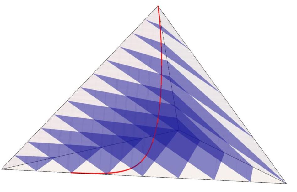
where $\theta^{*}$ satisfies the condition $\mbox{\boldmath$a$}^{\top}\mbox{\boldmath$p$}_{\theta^{*}}^{(q)}=C$. This foliation provides a geometric perspective on the simplex: each hyperplane ${\mathcal{H}}_{\mbox{\scriptsize\boldmath$a$}}(C)$ forms a ”leaf,” and the distribution of these leaves varies smoothly over $\Delta_{S-1}$. At every point within a leaf, the tangent space of the leaf aligns with a smoothly varying distribution over the simplex. Fig. 4 gives a 3D plot of the foliation in a $3$-dimensional simplex $\Delta_{3}$. We observe that the curve represents the ray ${\mathcal{P}}_{\mbox{\scriptsize\boldmath$a$}}$ that intersects the leaves ${\mathcal{H}}_{\mbox{\scriptsize\boldmath$a$}}(C)$’s at the conditional maximum points, in which the leaves are parallel to each other.

References

- Amari (1982) Amari, S. I. Differential geometry of curved exponential families: curvatures and information loss. The Annals of Statistics, 10(2):357–385, 1982.
- Amari and Nagaoka (2000) Amari, S. I., & Nagaoka, H. Methods of information geometry (Vol. 191). American Mathematical Soc., 2000.
- Basu et al. et al. (1998) Basu, A., Harris, I. R., Hjort, N. L. and Jones, M. C. Robust and efficient estimation by minimising a density power divergence. Biometrika, 85(3):549–559, 1998.
- Botta-Dukát (2005) Botta-Dukát, Z. Rao’s quadratic entropy as a measure of functional diversity based on multiple traits. Journal of vegetation science, 16(5), 533-540, 2005.
- Burbea and Rao (1982) Burbea, J. & Rao, C. R. On the convexity of some divergence measures based on entropy functions. IEEE Transactions on Information Theory, 28(3):489–495, 1982.
- Chao (1987) Chao, A. Estimating the population size for capture-recapture data with unequal matchability. Biometrics 43, 783-791, 1987.
- Colwell and Coddington (1994) Colwell, R. K. & Coddington, J. A. Estimating terrestrial biodiversity through extrapolation. Philosophical Transactions of the Royal Society of London. Series B: Biological Sciences, 345, 101-118, 1994.
- Dostál (2009) Dostál, Zdenek Optimal quadratic programming algorithms: with applications to variational inequalities,23, 2009, Springer Science & Business Media.
- Efron (1975) Efron, B. Defining the curvature of a statistical problem (with applications to second order efficiency). The Annals of Statistics, pages 1189–1242, 1975.
- Eguchi (1983) Eguchi, S. Second order efficiency of minimum contrast estimators in a curved exponential family. The Annals of Statistics, 793-803, 1983.
- Eguchi (1992) Eguchi, S. Geometry of minimum contrast. Hiroshima Mathematical Journal, 22(3):631–647, 1992.
- Eguchi and Copas (2006) Eguchi, S. and Copas, J. Interpreting Kullback–Leibler divergence with the Neyman–Pearson lemma. Journal of Multivariate Analysis, 97(9):2034–2040, 2006.
- Eguchi (2024) Eguchi, S. Minimum Gamma Divergence for Regression and Classification Problems. arXiv preprint arXiv:2408.01893, 2024.
- Eguchi and Komori (2022) Eguchi, S. and Komori, O. Minimum divergence methods in statistical machine learning: From an Information Geometric Viewpoint. Springer Japan KK, 2022.
- Eguchi et al. (2011) Eguchi, E., Komori, O. and Kato, S. Projective power entropy and maximum tsallis entropy distributions. Entropy, 13(10):1746–1764, 2011.
- Elith and Leathwick (2009) Elith, J. and Leathwick, J. R. Species distribution models: ecological explanation and prediction across space and time. Annual review of ecology, evolution, and systematics, 40(1):677–697, 2009.
- Fujisawa and Eguchi (2008) Fujisawa, H. and Eguchi, S. Robust parameter estimation with a small bias against heavy contamination. Journal of Multivariate Analysis, 99:2053–2081, 2008.
- Hill (1973) Hill, M. O. Diversity and evenness: a unifying notation and its consequences. Ecology 54, 427-432, 1973.
- Jost (2006) Jost, L. Entropy and diversity. Oikos, 113(2), 363-375, 2006.
- Komori and Eguchi (2019) Komori, O. and Eguchi, S. Statistical Methods for Imbalanced Data in Ecological and Biological Studies. Springer, Tokyo, 2019.
- Kusumoto et al. (2023) Kusumoto, B., Chao, A., Eiserhardt, W. L., Svenning, J. C., Shiono, T., & Kubota, Y. Occurrence-based diversity estimation reveals macroecological and conservation knowledge gaps for global woody plants. Science Advances, 9(40), eadh9719, 2023.
- May (1975) May, R. M. Patterns of species abundance and diversity. In Ecology and Evolution of Communities (ed. M. L. D. Cody, J. M.). Cambridge, Mass.: Harvard University Press, 1975.
- Leinster and Cobbold (2012) Leinster, T., & Cobbold, C. A. Measuring diversity: the importance of species similarity. Ecology, 93(3), 477-489, 2012.
- Nielsen (2021) Nielsen, F. On geodesic triangles with right angles in a dually flat space. In Progress in Information Geometry: Theory and Applications, pages 153–190. Springer, 2021.
- Phillips et al. (2004) Phillips, S. J., Dudík, M. and Schapire, R. E. A maximum entropy approach to species distribution modeling. In Proceedings of the twenty-first international conference on Machine learning, page 83, 2004.
- Rao (1945) Rao, C. R. Information and accuracy attainable in the estimation of statistical parameters. Bulletin of the Calcutta Mathematical Society, 37(3), 81-91, 1945.
- Rao (1961) Rao, C. R. Asymptotic efficiency and limiting information. In Proceedings of the Fourth Berkeley Symposium on Mathematical Statistics and Probability, Volume 1: Contributions to the Theory of Statistics, 4, 531-546, 1961. University of California Press.
- Rao (1982a) Rao, C. R. Diversity and dissimilarity coefficients: a unified approach. Theoretical population biology, 21(1), 24-43, 1982.
- Rao (1982b) Rao, C. R. Diversity: Its measurement, decomposition, apportionment and analysis. Sankhyā: The Indian Journal of Statistics, Series A, 1-22, 1982.
- Rao (1987) Rao, C. R. Differential metrics in probability spaces. Differential geometry in statistical inference, 10:217–240, 1987.
- Saigusa et al. (2024) Saigusa, Y., Eguchi, S. and Komori, O. Robust minimum divergence estimation in a spatial Poisson point process. Ecological Informatics, 81:102569, 2024.
- Simpson (1949) Simpson, E. H. Measurement of diversity. Nature 163, 688, 1949.
- Southwood and Henderson (2009) Southwood, T. R. E., & Henderson, P. A. Ecological methods. John Wiley & Sons, 2009.
Appendix
We explore the ranges of for defining a mixture geodesic and -geodesic in .
Proposition 6.
Consider a mixture geodesic connecting and in the interior of , where . The range of is enlarged to a closed interval
where
Proof.
By definition,