Information Thermodynamics of the Transition-Path Ensemble
Abstract
The reaction coordinate describing a transition between reactant and product is a fundamental concept in the theory of chemical reactions. Within transition-path theory, a quantitative definition of the reaction coordinate is found in the committor, which is the probability that a trajectory initiated from a given microstate first reaches the product before the reactant. Here we develop an information-theoretic origin for the committor and show how selecting transition paths from a long ergodic equilibrium trajectory induces entropy production which exactly equals the information that system dynamics provide about the reactivity of trajectories. This equality of entropy production and dynamical information generation also holds at the level of arbitrary individual coordinates, providing parallel measures of the coordinate’s relevance to the reaction, each of which is maximized by the committor.
Understanding the mechanism for a transition between metastable states of a system is of fundamental interest to the natural sciences. Reaction theories seek to derive the rate constant from underlying system dynamics and have led to increased insight into the reaction mechanism, the sequence of elementary steps by which a reaction occurs. A notable example is transition-state theory and its extensions Eyring (1935); Evans and Polanyi (1935); Kramers (1940), which conceptualize the activated complex (or transition-state species) as a key dynamical intermediate and makes use of its properties (e.g., free energy relative to the reactant) to derive an approximate rate constant for large classes of reactions. The transition state is one identifiable state along the reaction coordinate, a one-dimensional collective variable that preserves all quantitative and qualitative aspects of a reaction under projection of the multidimensional dynamics Peters (2016); Bolhuis and Dellago (2015).
Motivated by rare-event sampling methods Dellago et al. (1998), transition-path theory E and Vanden-Eijnden (2006) was developed to quantitatively describe the entire reaction and determine its rate constant, without assumptions of metastability for the reactant and product or any specific details of the reaction mechanism (e.g., the presence of a single transition state). This statistical description relies on the definition of the committor function (also called the commitment or splitting probability), the probability that a trajectory initiated from microstate reaches the product before returning to the reactant. The committor maps the state space onto the interval and has been called the “true” or “ideal” one-dimensional reaction coordinate Peters (2016); E and Vanden-Eijnden (2010); Li and Ma (2014); Peters et al. (2013); Banushkina and Krivov (2016). The committor allows calculation of the reaction rate from a one-dimensional description Berezhkovskii and Szabo (2013) and identifies the transition-state ensemble as states making up the isocommittor surface Berezhkovskii and Szabo (2005).
In this Letter, we derive a novel information-theoretic justification of the committor as the reaction coordinate. We show how selecting the transition-path ensemble (the set of trajectories from reactant to product) from a long ergodic equilibrium trajectory results in entropy production that precisely equals the information generated by system dynamics about the reactivity of trajectories.
The components of entropy production and information generation due to an arbitrary system coordinate are also equal; this reveals equivalent thermodynamic and information-theoretic measures of the suitability of low-dimensional collective variables that encode information relevant for describing reaction mechanisms. The committor is a single coordinate that preserves all system entropy production and distills all system information about reactivity, giving further support for its role as the reaction coordinate.
Information-theoretic formulation of the committor as reaction coordinate.—Consider a multidimensional system evolving according to Markovian dynamics governed by the master equation Zwanzig (2001), , where is the transition rate from state and is the probability of state . We assume the transition rates obey detailed balance Zwanzig (2001) and the system is in equilibrium with its environment so that , the equilibrium probability of . We study the transition-path ensemble (TPE), the set of trajectories that leave one subset of states and next visit a distinct subset before . In most applications, and are metastable states separated by a dynamical barrier; following Refs. Metzner et al. (2009); Vanden-Eijnden (2014), we only assume that and do not overlap and lack direct transitions, i.e., for and .
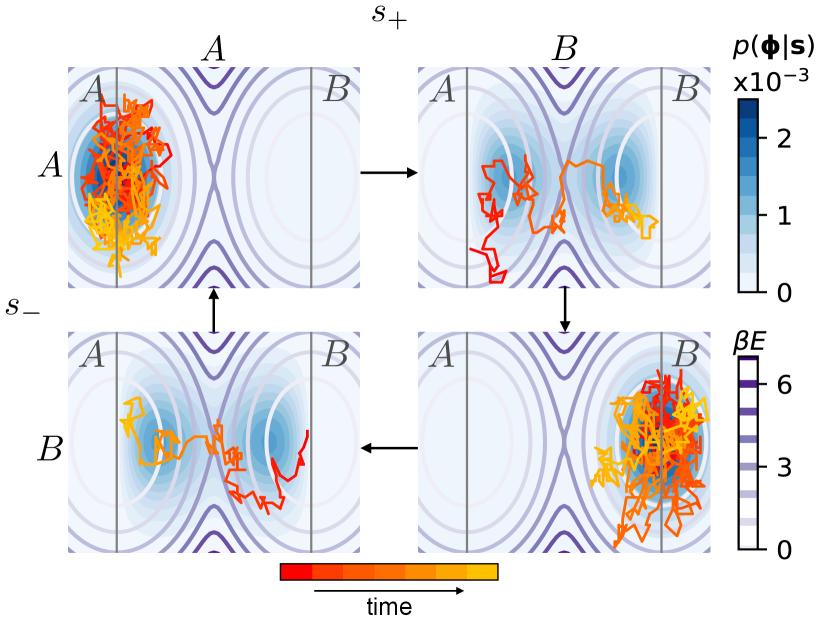
The TPE can be formed by selecting from a long ergodic equilibrium supertrajectory the trajectory segments that leave and reach before . Transition paths are therefore selected based on the trajectory outcome (the next mesostate ( or ) visited by the system) and origin (the mesostate most recently visited by the system). This partitions the supertrajectory into four trajectory subensembles, each with particular : The forward (reverse) transition-path ensemble is the set of trajectory segments with [], and the stationary subensemble from () has [], as depicted in Fig. 1. Every trajectory segment in the forward TPE has a corresponding equally probable time-reversed trajectory segment in the reverse TPE.
At any time during the equilibrium supertrajectory, we define random variables and , respectively, denoting the current system state and trajectory subensemble, with the joint distribution that the system is currently in state and is currently on a trajectory segment with respective origin and outcome . Since the system dynamics are Markovian, the trajectory outcome and origin are conditionally independent given current state , so the joint distribution can be factored as Metzner et al. (2009). The conditional probabilities of trajectory outcome and origin given current state are
| (1a) | ||||
| (1b) | ||||
Here is the forward committor, the probability that the system currently in state will next reach before , and is the backward committor, the probability that the system (currently in ) was more recently in mesostate than in . The committors obey boundary conditions and for , and and for . Since the system is in equilibrium and the transition rates obey detailed balance, Metzner et al. (2009), a single committor (without loss of generality, the forward committor ) provides information about both the outcome and origin of the trajectory segment, so we refer to as the reaction coordinate.
During the equilibrium supertrajectory, the system continually evolves from to and to , completing a unidirectional cycle through each subensemble with stochastic transition times depending on underlying microscopic dynamics. Transition-path theory Vanden-Eijnden (2014); Berezhkovskii and Szabo (2019); E and Vanden-Eijnden (2006) derives quantitative properties (reaction rate and free-energy difference) of the reaction from the equilibrium probability flux of subensemble transitions
| (2) |
and the respective marginal probabilities and :
| (3a) | |||||||||
| (3b) | |||||||||
| (3c) | |||||||||
where () is the rate constant for the () transition and is the free-energy difference. Mesoscopic reaction properties are therefore derived from information about the subensembles, specifically the proportion of time spent in each subensemble and how frequently the subensemble switches.
The reaction coordinate should be maximally informative about the current subensemble. This is precisely quantified by mutual information, a nonlinear statistical measure of the relationship between two random variables, specifically quantifying the reduction of uncertainty (given by Shannon entropy ) about one random variable from measuring another Cover and Thomas (2006):
| (4) |
where is the marginal probability that the system is currently on a trajectory segment with outcome and origin . Operationally, can be estimated from the proportion of time spent in subensemble during an equilibrium supertrajectory of length , . If the committor depends only on a one-dimensional coordinate (i.e. ), then is a sufficient statistic for the mutual information between trajectory subensemble and full system state, i.e., . In this sense, the committor is the “optimal” reaction coordinate, since it is maximally informative about the trajectory subensemble given a measurement of system state. This is our first major result.
Physically, the trajectory outcome and origin (and hence the committors) represent uncertainty in the state of the environment. Classical mechanics assumes a constant-energy universe (system plus environment ) governed by deterministic dynamics so that the outcome and origin of the trajectory initiated from a given state of system and environment are deterministic (and can be determined by integrating the state of the universe forward and backward in time until the system reaches or ), i.e., is either 0 or 1. This partitions the state space of the universe into four quadrants corresponding to each trajectory subensemble, with each state belonging to only one subensemble; thus the uncertainty about the trajectory subensemble given a state of the universe is zero, . In this case, the mutual information between the universe and trajectory subensemble is the uncertainty about the trajectory subensemble, ; the measurement of the state of the universe fully determines the trajectory outcome and origin.
However, we typically do not resolve the microstate of the environment, instead coarse-graining its interaction with the system into friction and fluctuations Zwanzig (2001). Measurement of the system state alone does not fully determine the trajectory outcome and origin, which become random variables with positive conditional Shannon entropy reflecting uncertainty in the state of the environment that is relevant to classification of the current subensemble.
Transition-path thermodynamics.—The joint dynamics of is given by the master equation
| (5) |
where the transition rate is (see Supplemental Material I SM )
| (6) |
The top transition does not change the subensemble, and biases transitions within subensemble toward states with higher probability of trajectory outcome . The middle four transitions switch subensembles and are unidirectional, contributing to the probability flux [Eq. (2) and Supplemental Material Eq. (S9)]. These joint dynamics are Markovian: Since the underlying system dynamics are Markovian, the transition rates (6) do not depend on the trajectory origin , and the outcome does not induce dependence on earlier system states. Considered alone, system dynamics are at equilibrium and microscopically reversible; adding the trajectory outcome and origin variables (that are not functions of system state and explicitly depend on the past and future) breaks time-reversal symmetry, producing absolutely irreversible trajectory-subensemble transitions and time-asymmetric system transitions within a given subensemble.
To quantify the time asymmetry for a particular transition in subensemble , we combine (6) Bayes’ rule, and the equilibrium detailed-balance relation to derive a local detailed-balance relation,
| (7) |
The (and analogously ) stationary subensemble has , and due to system detailed balance , so the rhs is unity and detailed balance holds for transitions within stationary subensembles. The reactive subensembles (forward or reverse TPE) have different trajectory outcome and origin so the rhs side differs from unity, leading to a detailed-balance-breaking flux (and hence entropy production) along particular transitions within these subensembles.
Within a fixed subensemble , the net trajectory flux is
| (8a) | ||||
| (8b) | ||||
The second equality follows from ; the conditional independence of and given state , i.e., ; and substitution for using (6). The stationary subensembles ( and ) have no net flux because each trajectory segment and its time-reversed counterpart occur at equal rates within the same subensemble. In contrast, the forward and reverse TPEs have net trajectory flux since each transition path and its time-reversed counterpart occur in different subensembles. (Our procedure of effectively replicating the state space and introducing opposing fluxes in the replicas by modification of the transition rates bears similarity to nonreversible Markov chains obeying skew detailed balance used to speed convergence to a stationary distribution Turitsyn et al. (2011).)
We decompose (see Supplemental Material II SM ) the change in joint entropy at steady state Busiello et al. (2020); Esposito (2012) into
| (9a) | ||||
| (9b) | ||||
where is the subensemble-weighted average of the irreversible entropy production rate conditioned on subensemble , which quantifies the time irreversibility of system dynamics within that subensemble. is the rate of change in mutual information between the trajectory outcome and system state due to system dynamics in a fixed subensemble Horowitz and Esposito (2014). Rearranging Eq. (9b) gives (see Supplemental Material III SM ):
| (10a) | ||||
| (10b) | ||||
where is the rate of change in mutual information between trajectory origin and system state due to dynamics in a fixed subensemble. These information rates reflect the dependence of the trajectory outcome and origin variables on the past and future states of the system: As the system evolves, uncertainty about the outcome diminishes, increasing the information the current system state carries about , while uncertainty (given current system state ) about the origin increases, decreasing information carries about the .
Since the stationary subensembles have no entropy production (), Eq. (10a) reduces to an equation for a single subensemble,
| (11) |
This equates the rate of generating information about the outcome with the product of the entropy production rate of a reactive subensemble and that subensemble’s marginal probability . Although the supertrajectory is at equilibrium with no entropy production, physically represents the dissipation that would be necessary in a system evolving according to the TPE’s detailed-balance-breaking transition rates (top line of (6) for ). Equation (11) is our second major result: The entropy production in a reactive subensemble equals the information generated about the reactivity of trajectories.
When the state space is continuous, we derive (see Supplemental Material IV SM ) a Fisher-information metric that imposes an information geometry on the state space Amari (2016); Nielsen (2020). The metric measures distance on the reaction coordinate (committor) as the system evolves and thereby defines a reaction-coordinate length . From this, the TPE entropy production is
| (12) |
where is the mean duration of a transition path. This relates the TPE entropy production to the squared length between and along the reaction coordinate.
Bipartite dynamics.—We now demonstrate how the TPE entropy production quantitatively measures the relevance of an arbitrary coordinate to the reaction. We assume bipartite dynamics Hartich et al. (2014); Barato et al. (2013), essentially that instantaneous transitions only happen in either a one-dimensional coordinate or in all other degrees of freedom making up the system state :
| (13) |
Dynamics that do not obey the bipartite assumption introduce further complications in unambiguously partitioning the entropy production between coordinates Chetrite et al. (2019).
Combining Eqs. (1), (8a), and (9b) gives the full TPE entropy production as a function of the forward committor,
| (14) |
which splits into contributions from the two transition types:
| (15a) | |||
| (15b) | |||
The same decomposition holds for the information rate Horowitz and Esposito (2014), so that TPE entropy production due to dynamics is equal to the information rate (due to dynamics) between and :
| (16) |
This is our third major result: The entropy production due to dynamics of coordinate equals the mutual information generated by dynamics, thereby quantifying the relevance of transitions to identifying the current subensemble and highlighting those transitions that are “correlated” with reactive trajectories and therefore important to the reaction mechanism.
In particular, for determining the committor and orthogonal degrees of freedom that are therefore not relevant to the reaction (), the entropy production rate due to dynamics is [simplifying Eq. (15b)]:
| (17a) | ||||
| (17b) | ||||
Therefore . This is additional confirmation that the committor is the reaction coordinate, in that it provides a thermodynamically complete coarse-grained representation of the transition-path ensemble, fully accounting for its entropy production Esposito (2012).
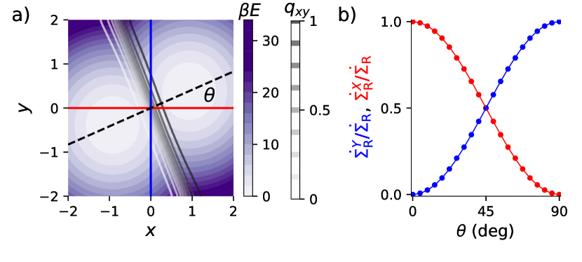
We illustrate with overdamped dynamics in a double-well energy landscape [Fig. 2(a), details in Supplemental Material V SM ]. To exemplify the typical situation where the reaction coordinate is not known a priori and coordinates are thus chosen based on convenience or intuition, fixed system coordinates lie at an angle to the correct reaction coordinate, the linear coordinate passing through both energy minima. For , is the reaction coordinate, is an orthogonal bath mode Li and Ma (2016), and dynamics fully capture the TPE entropy production without contribution. Figure 2(b) shows that as the underlying energy landscape is rotated relative to system coordinates, the -coordinate entropy production decreases and -coordinate entropy production increases, with equal contribution at . The entropy production for each coordinate is proportional to the squared Euclidean distance between and projected onto each coordinate, and .
Discussion.—We have derived the information thermodynamics of a system undergoing reactions between distinct state-space subsets and , making a fundamental connection between transition-path theory, information theory, and stochastic thermodynamics. Partitioning a long ergodic equilibrium trajectory into reactive and nonreactive subensembles results in entropy production for system dynamics in the reactive subensembles (physically representing the dissipation needed to implement the detailed-balance-breaking transition rates of the TPE), which in turn identifies transitions that are relevant to the overall reaction mechanism. This rigorous equality between TPE entropy production and informativeness of dynamics also holds for an arbitrary coordinate, revealing parallel stochastic-thermodynamic and information-theoretic measures of the relevance of collective variables to the system reaction, that are each maximized by the committor.
This work has implications for the identification of important collective variables and analysis of reaction mechanisms. While the committor provides a microscopically detailed reaction coordinate that maps each system microstate to a scalar value, it does not immediately identify physically meaningful collective variables (e.g., internal molecular coordinates) that are relevant to the reaction Bolhuis and Dellago (2015); Peters (2016); Johnson and Hummer (2012). Our results have indicated that relevant coordinates are identified by entropy production in the transition-path ensemble; thus partitioning the entropy production between multiple relevant collective variables for which one has physical intuition can provide a low-dimensional model that allows increased insight into the reaction mechanism.
More concretely, this connection we have established between transition-path theory and stochastic thermodynamics suggests a novel method for rigorously grounded inference of reaction coordinates: generate an ensemble of transition paths using transition-path sampling Dellago et al. (1998); Bolhuis et al. (2002) or related algorithms Van Erp et al. (2003); Allen et al. (2005); Faradjian and Elber (2004); estimate entropy production along chosen coordinates Seifert (2019); Li et al. (2019a); Skinner and Dunkel (2021) or identify linear combinations of coordinates producing the most entropy using dissipative components analysis Gnesotto et al. (2020); use these most dissipative coordinates to enhance sampling of transition paths; and through further iteration identify system coordinates producing the most entropy in the transition-path ensemble and hence of most relevance to the reaction.
Machine-learning approaches to solve for high-dimensional committor coordinates Khoo et al. (2019); Li et al. (2019b); Rotskoff et al. or find low-dimensional reaction models that retain predictive power Ma and Dinner (2005); Wang and Tiwary (2021) are active areas of research Wang et al. (2020). The information-theoretic and thermodynamic perspectives on reactive trajectories described in this Letter provide guidance to the development of data-intensive automated methods to infer these models and their corresponding reaction mechanisms.
This work was supported by Natural Sciences and Engineering Research Council of Canada (NSERC) Canada Graduate Scholarships Masters and Doctoral (MDL), an NSERC Discovery Grant (DAS), and a Tier-II Canada Research Chair (DAS). The authors thank Jannik Ehrich (SFU Physics) for enlightening feedback on the manuscript.
References
- Eyring (1935) H. Eyring, J. Chem. Phys. 3, 107 (1935).
- Evans and Polanyi (1935) M. G. Evans and M. Polanyi, Trans. Faraday Soc. 31, 875 (1935).
- Kramers (1940) H. A. Kramers, Physica 7, 284 (1940).
- Peters (2016) B. Peters, Annu. Rev. Phys. Chem 67, 669 (2016).
- Bolhuis and Dellago (2015) P. G. Bolhuis and C. Dellago, Eur. Phys. J. Spec. Top. 224, 2409 (2015).
- Dellago et al. (1998) C. Dellago, P. G. Bolhuis, F. S. Csajka, and D. Chandler, J. Chem. Phys. 108, 1964 (1998).
- E and Vanden-Eijnden (2006) W. E and E. Vanden-Eijnden, J. Stat. Phys. 123, 503 (2006).
- E and Vanden-Eijnden (2010) W. E and E. Vanden-Eijnden, Annu. Rev. Phys. Chem 61, 391 (2010).
- Li and Ma (2014) W. Li and A. Ma, Mol Simul. 40, 784 (2014).
- Peters et al. (2013) B. Peters, P. G. Bolhuis, R. G. Mullen, and J.-E. Shea, J. Chem. Phys. 138, 054106 (2013).
- Banushkina and Krivov (2016) P. V. Banushkina and S. V. Krivov, WIREs Comput Mol Sci 6, 748 (2016).
- Berezhkovskii and Szabo (2013) A. M. Berezhkovskii and A. Szabo, J. Phys. Chem. B 117, 13115 (2013).
- Berezhkovskii and Szabo (2005) A. Berezhkovskii and A. Szabo, J. Chem. Phys. 122, 014503 (2005).
- Zwanzig (2001) R. Zwanzig, Nonequilibrium statistical mechanics (Oxford University Press, New York, 2001).
- Metzner et al. (2009) P. Metzner, C. Schutte, and E. Vanden-Eijnden, SIAM Multiscale Model. Simul. 7, 1192 (2009).
- Vanden-Eijnden (2014) E. Vanden-Eijnden, in An introduction to Markov state models their application to long timescale molecular simulation, edited by G. R. Bowman, V. S. Pande, and F. Noe (Springer, 2014), chap. 7, pp. 91–100.
- Berezhkovskii and Szabo (2019) A. M. Berezhkovskii and A. Szabo, J. Chem. Phys 150, 054106 (2019).
- Cover and Thomas (2006) T. M. Cover and J. A. Thomas, Elements of information theory (John Wiley & Sons, Inc., Hoboken, New Jersey, 2006), 2nd ed.
- (19) See Supplemental Material at [URL will be inserted by publisher].
- Turitsyn et al. (2011) K. S. Turitsyn, M. Chertkov, and M. Vucelja, Physica D 240, 410 (2011).
- Busiello et al. (2020) D. M. Busiello, D. Gupta, and A. Maritan, Phys. Rev. Res. 2, 1 (2020).
- Esposito (2012) M. Esposito, Phys. Rev. E 85, 041125 (2012).
- Horowitz and Esposito (2014) J. M. Horowitz and M. Esposito, Phys. Rev. X 4, 031015 (2014).
- Amari (2016) S.-I. Amari, Information geometry and its applications (Springer, Tokyo, 2016), 1st ed.
- Nielsen (2020) F. Nielsen, Entropy 22, 1100 (2020).
- Hartich et al. (2014) D. Hartich, A. Barato, and U. Seifert, J. Stat. Mech Theory Exp. 2014, 02016 (2014).
- Barato et al. (2013) A. C. Barato, D. Hartich, and U. Seifert, J Stat Phys 153 (2013).
- Chetrite et al. (2019) R. Chetrite, M. L. Rosinberg, T. Sagawa, and G. Tarjus, J. Stat. Mech. 21, 114002 (2019).
- Li and Ma (2016) W. Li and A. Ma, J. Chem. Phys. 144, 114103 (2016).
- Johnson and Hummer (2012) M. E. Johnson and G. Hummer, J. Phys. Chem. B 116, 8573 (2012).
- Bolhuis et al. (2002) P. G. Bolhuis, D. Chandler, C. Dellago, and P. L. Geissler, Annu. Rev. Phys. Chem 53, 291 (2002).
- Van Erp et al. (2003) T. S. Van Erp, D. Moroni, and P. G. Bolhuis, J. Chem. Phys. 118, 6617 (2003).
- Allen et al. (2005) R. J. Allen, P. B. Warren, and P. R. Ten Wolde, Phys. Rev. Lett. 94, 018104 (2005).
- Faradjian and Elber (2004) A. K. Faradjian and R. Elber, J. Chem. Phys. 120, 10880 (2004).
- Seifert (2019) U. Seifert, Annu. Rev. Condens. Matter Phys. 10, 171 (2019).
- Li et al. (2019a) J. M. Li, Junang andHorowitz, T. R. Gingrich, and N. Fakhri, Nature Communications 10 (2019a).
- Skinner and Dunkel (2021) D. J. Skinner and J. Dunkel, PNAS 118 (2021).
- Gnesotto et al. (2020) F. S. Gnesotto, G. Gradziuk, P. Ronceray, and C. P. Broedersz, Nat. Commun. 11, 5378 (2020).
- Khoo et al. (2019) Y. Khoo, J. Lu, and L. Ying, Res. Math. Sci. 6, 1 (2019).
- Li et al. (2019b) Q. Li, B. Lin, and W. Ren, J. Chem. Phys. 151, 54112 (2019b).
- (41) G. M. Rotskoff, A. R. Mitchell, and E. Vanden-Eijnden, arXiv:2008.06334v2.
- Ma and Dinner (2005) A. Ma and A. R. Dinner, J. Phys. Chem. B 109, 6769 (2005).
- Wang and Tiwary (2021) Y. Wang and P. Tiwary, J. Chem. Phys. 154, 134111 (2021).
- Wang et al. (2020) Y. Wang, J. M. L. Ribeiro, and P. Tiwary, Curr. Opin. Struct. Biol. 61, 139 (2020).
- Ito (2018) S. Ito, Phys. Rev. Lett. 121, 30605 (2018).
- Ruppeiner (1979) G. Ruppeiner, Phys. Rev. A 20, 1608 (1979).
- Crooks (2007) G. E. Crooks, Phys. Rev. Lett. 99, 100602 (2007).
- Metropolis et al. (1953) N. Metropolis, A. W. Rosenbluth, M. N. Rosenbluth, A. H. Teller, and E. Teller, J. Chem. Phys. 21, 1087 (1953).
Supplemental Material for “Information Thermodynamics of the Transition-Path Ensemble”
I Joint transition rates
Following Vanden-Eijnden (2014), the transition probability over time for a transition given the trajectory remains in subensemble is
| (S1a) | ||||
| (S1b) | ||||
| (S1c) | ||||
| (S1d) | ||||
| (S1e) | ||||
| (S1f) | ||||
(S1b) splits the joint probability into conditional and marginal probabilities. In (S1c), we recognize that when the subensemble doesn’t change. In (S1d), we use the Markov property to eliminate the dependence of the next state on trajectory origin. In (S1e), we express the conditional probability as the ratio of joint and marginal probabilities. In (S1f), we recognize that the trajectory outcome depends only on the most recent state and drop the dependency on . Finally, we recall that for these transitions and re-express the transition probability as a transition rate,
| (S2) |
We similarly derive transition rates for the four sets of transitions that change subensemble, where either the trajectory origin or outcome changes while the other is constant. The transition probability in time for a transition out of where the subensemble changes from is:
| (S3a) | ||||
| (S3b) | ||||
| (S3c) | ||||
| (S3d) | ||||
(S3c) uses the fact that when . (S3d) uses the Markov property to simplify the conditional distributions. We then re-express the transition probability as a transition rate
| (S4) |
Similarly, the transition rate for a transition where the subensemble outcome changes from is
| (S5) |
The trajectory origin changes when the system finishes a transition path at the boundary of or . The probability for a transition into where the subensemble changes from is:
| (S6a) | ||||
| (S6b) | ||||
| (S6c) | ||||
| (S6d) | ||||
| (S6e) | ||||
| (S6f) | ||||
(S6c) recognizes that and for and uses the Markov property to eliminate dependence on in . (S6f) uses for . Finally, we re-express the transition probability as the transition rate
| (S7) |
and similarly derive the transition rate for a transition where the system enters and finishes a forward TPE () as
| (S8) |
These rates are explicitly written for each transition in (2), and when averaged over all such transitions yield the unidirectional probability flux between trajectory subensembles (3),
| (S9a) | ||||
| (S9b) | ||||
| (S9c) | ||||
| (S9d) | ||||
Note that each RHS of (S9) has an implicit conditional probability for the other element of the trajectory subsensemble, each of which equals unity on the relevant system subspace, e.g., for in (S9a).
II Entropy production for joint dynamics in
We decompose the change in joint entropy (9a) into three terms Busiello et al. (2020)
| (S10a) | ||||
where is the irreversible entropy production and the environmental entropy change for transitions that do not change the subensemble, and is the change in joint entropy due to transitions that change the subensemble.
The transitions that change the trajectory subensemble do not change joint entropy:
| (S11a) | ||||
| (S11b) | ||||
In (S11a), the first and second terms and the third and fourth terms cancel because of the equilibrium relationships , , and .
We express the irreversible entropy production in terms of the irreversible entropy production of dynamics given fixed subensemble , Esposito (2012):
| (S12a) | ||||
| (S12b) | ||||
| (S12c) | ||||
Finally, the environmental entropy change is
| (S13a) | ||||
| (S13b) | ||||
| (S13c) | ||||
where we get (S13b) by summing over the trajectory origin.
III Mutual information rates between system state and either trajectory outcome or trajectory origin have equal magnitude
The rate of change in mutual information between system state and trajectory outcome due to dynamics is of equal magnitude and opposite sign from the rate of change in mutual information between system state and trajectory origin due to dynamics:
| (S14a) | ||||
| (S14b) | ||||
| (S14c) | ||||
| (S14d) | ||||
| (S14e) | ||||
| (S14f) | ||||
In (S14b) we expand the joint transition rate using (6); (S14c) relates outcome and origin probabilities using equilibrium relations , ; and (S14d) uses detailed balance, .
IV Thermodynamic metric
Here we assume that the state space is continuous, and the master equation represents a discrete approximation of its dynamics. We rearrange the difference in mutual information rates (10b) to obtain the transition-weighted relative entropy between the conditional subensemble distributions and before and after the transition, respectively, then expand in small state changes :
| (S15a) | ||||
| (S15b) | ||||
| (S15c) | ||||
| (S15d) | ||||
| (S15e) | ||||
| (S15f) | ||||
In (S15c), we multiply each term by unity ( and respectively), then use detailed balance () to combine terms in (S15d). is the th component of the state-space vector and is the Fisher information of the trajectory outcome/origin distribution at state ,
| (S16a) | ||||
| (S16b) | ||||
| (S16c) | ||||
| (S16d) | ||||
| (S16e) | ||||
In (S16), we write out each term from (S16b) in terms of the forward committor . We use the chain rule to pull out a common factor in (S16d) and simplify in (S16e).
In information geometry Amari (2016); Nielsen (2020), Fisher information arises as a distance metric in the parameter space of a probability distribution. Here, we consider changes in conditional probability as the system evolves, where the system state parameterizes the conditional probability distribution through the committor . When the system is in (), there is no uncertainty about trajectory outcome and origin , so the conditional probability () is unity for () and zero for all other subensembles. As the system evolves, the distribution corresponding to the current system state changes, and the information-geometric distance between successive distributions is quantified by the Fisher information metric, with square line element Ito (2018)
| (S17) |
Equation (S15f) is then the rate of mean square distance accumulated by the system evolving at equilibrium,
| (S18) |
Multiplying by the mean round-trip time through the subensembles (the sum of mean first-passage times from to and to Berezhkovskii and Szabo (2019)), we obtain the squared reaction-coordinate length as the mean square metric distance for a round trip :
| (S19a) | ||||
| (S19b) | ||||
| (S19c) | ||||
| (S19d) | ||||
for mean transition-path duration . The reaction-coordinate length roughly quantifies the mean number of fluctuations Ruppeiner (1979); Crooks (2007) required for the system to complete a round trip.
V Computational details
The bistable energy potential is separable into terms only depending on the reaction coordinate and on the bath mode :
| (S20) |
where defines the locations of the energy minima. is the landscape curvature near those energy minima, chosen such that the energy barrier is .
We represent the system state with orthogonal coordinates , related to by rotational angle :
| (S21a) | ||||
| (S21b) | ||||
We discretize the state space so that , and dynamically evolve bipartite dynamics using the master equation. The transition rate is with diffusion prefactor and energy change Metropolis et al. (1953). We solve the committor on the discrete state space using the recursion relations Metzner et al. (2009)
| (S22a) | ||||
| (S22b) | ||||
Mesostates are defined by and , so that the committor is independent of . We calculate the TPE entropy production from (15).