Initial-Value Privacy of Linear Dynamical Systems
Abstract
This paper studies initial-value privacy problems of linear dynamical systems. We consider a standard linear time-invariant system with random process and measurement noises. For such a system, eavesdroppers having access to system output trajectories may infer the system initial states, leading to initial-value privacy risks. When a finite number of output trajectories are eavesdropped, we consider a requirement that any guess about the initial values can be plausibly denied. When an infinite number of output trajectories are eavesdropped, we consider a requirement that the initial values should not be uniquely recoverable. In view of these two privacy requirements, we define differential initial-value privacy and intrinsic initial-value privacy, respectively, for the system as metrics of privacy risks. First of all, we prove that the intrinsic initial-value privacy is equivalent to unobservability, while the differential initial-value privacy can be achieved for a privacy budget depending on an extended observability matrix of the system and the covariance of the noises. Next, the inherent network nature of the considered linear system is explored, where each individual state corresponds to a node and the state and output matrices induce interaction and sensing graphs, leading to a network system. Under this network system perspective, we allow the initial states at some nodes to be public, and investigate the resulting intrinsic initial-value privacy of each individual node. We establish necessary and sufficient conditions for such individual node initial-value privacy, and also prove that the intrinsic initial-value privacy of individual nodes is generically determined by the network structure. These results may be extended to linear systems with time-varying dynamics under the same analysis framework.
1 Introduction
The rapid developments in networked control systems [1], internet of things [2, 3], smart grids [4], intelligent transportation [5, 6] during the past decade shed lights on how future infrastructures of our society can be made smart via interconnected sensing, dynamics, and control over cyber-physical systems. The operation of such systems inherently relies on users and subsystems sharing signals such as measurements, dynamical states, control inputs in their local views, so that collective decisions become possible. The shared signals might directly contain sensitive information of a private nature, e.g., loads and currents in a grid reflect directly activities in a residence or productions in a company [7]; or they might indirectly encode physical parameters, user preferences, economic inclination, e.g., control inputs in economic model predictive control implicitly carry information about the system’s economic objective as it is used as the objective function [8].
Several privacy metrics have been developed to address privacy expectations of dynamical systems. A notable metric is differential privacy, which originated in computer science[9, 10, 11]. When a mechanism is applied taking the sensitive information as input and producing an output as the learning outcome, differential privacy guarantees plausible deniability of any inference about the private information by eavesdroppers having access to the output. Differential privacy has become the canonical solutions for privacy risk characterization in dataset processing, due to its quantitative nature and robustness to post-processing and side information [10, 11]. The differential privacy framework has also been generalized to dynamical systems for problems ranging from average consensus seeking [12] and distributed optimization [13, 14] to estimation and filtering [15, 7] and feedback control [16, 17]. Consistent with its root, differential privacy for a dynamical system provides the system with the ability to have plausible deniability facing eavesdroppers, e.g., recent surveys in [19, 18].
Besides differential privacy, another related but different privacy risk lies in the possibility that an eavesdropper makes an accurate enough estimation of the sensitive parameters or signals, perhaps from a number of repeated observations. In [20], the variance matrix of the maximum likelihood estimation was utilized to measure how accurate the initial node states in a consensus network maybe estimated from the trajectories of one or more malicious nodes. In [21], a measure of privacy was developed using the inverse of the trace of the Fisher information matrix, which is a lower bound of the variance of estimation error of unbiased estimators.
In particular, initial values of a dynamical system may carry sensitive private information, leading to privacy risks related to the initial values. For instance, when distributed load shedding in micro-grid systems is performed by employing an average consensus dynamics, initial values represent load demands of individual users [22]. In [12, 20], the initial-value privacy of the average consensus algorithm over dynamical networks was studied, and injecting exponentially decaying noises was used as a privacy-protection approach. The privacy of the initial value for a dynamical system is also of significant theoretical interest as the system trajectories or distributions of the system trajectories are fully parametrized by the initial value, in the presence of the plant knowledge. In [21], the initial-value privacy of a linear system was studied, and an optimal privacy-preserving policy was established for the probability density function of the additive noise such that the balance between the Fisher information-based privacy level and output performance is achieved.
In this paper, we study initial-value privacy problems of linear dynamical systems in the presence of random process and sensor noises. For such a system, eavesdroppers having access to system output trajectories may infer the system initial states. When a finite number of output trajectories are eavesdropped, we consider a requirement that any guess about the initial values can be plausibly denied. When an infinite number of output trajectories are eavesdropped, we consider a requirement that the initial values should not be uniquely recoverable. These requirements inspire us to define and investigate two initial-value privacy metrics for the considered linear system: differential initial-value privacy on the plausible deniability, and intrinsic initial-value privacy on the fundamental non-identifiability. Next, we turn to the inherent network nature of linear systems, where each dimension of the system state corresponds to a node, and the state and output matrices induce interaction and sensing graphs. In the presence of malicious users or additional observations, the initial states at a subset of the nodes may be known to the eavesdroppers as well. With such a public disclosure set, the intrinsic initial-value privacy of each individual node, and the structural privacy metric of the entire network, become interesting and challenging questions.
The main results of this paper are summarized in the following:
-
•
For general linear systems, we prove that intrinsic initial-value privacy is equivalent to unobservability; and that differential initial-value privacy can be achieved for a privacy budget depending on an extended observability matrix of the system and the covariance of the noises.
-
•
For networked linear systems, we establish necessary and sufficient conditions for intrinsic initial-value privacy of individual nodes, in the presence of a public disclosure set consisting of nodes with known initial states. We also show that the network structure plays a generic role in determining the privacy of each node’s initial value, and the maximally allowed number of arbitrary disclosed nodes under privacy guarantee as a network privacy index.
These results may be extended to linear (network) systems with time-varying dynamics under the same analysis framework. The network privacy as proven to be a generic structural property, is a generalization to the classical structural observability results.
A preliminary version of the results is presented in [23] where the technical proofs, illustrative examples, and many discussions were not included. The remainder of the paper is organized as follows. Section 2 formulates the problem of interest for linear dynamical systems. In Section 3, intrinsic initial-value privacy and differential privacy are explicitly defined and studied by regarding all initial values as a whole. Then regarding the system from the network system perspective, Section 4 analyzes the intrinsic initial-value privacy of individual nodes with a public disclosure set and studies a quantitative network privacy index, from exact and generic perspectives. Finally a brief conclusion is made in Section 5. All technical proofs are presented in the Appendix.
Notations. We denote by the real numbers and the real space of dimension for any positive integer . For a vector , the norm . For any , we denote as a vector , and as a matrix of which the -the column is , . For any square matrix , let denote the set of all eigenvalues of , and denote the maximum and minimum eigenvalues, respectively. For any matrix , the norm . For any set , we let be a characteristic function, satisfying for and for . The range of a matrix or a function is denoted as , and the span of a matrix is denoted as . We denote as the probability density function, and as a vector whose entries are all zero except the -th being one.
2 Problem Statement
2.1 Initial-Value Privacy for Linear Systems
We consider the following linear time-invariant (LTI) system
| (1) |
for , where is state, is output, is process noise, and is measurement noise. Throughout this paper, we assume that and are random variables according to some zero-mean distributions, and .
In this paper, we suppose that initial values are privacy-sensitive information for the system. Eavesdroppers having access to the output trajectory with attempt to infer the private initial values. To facilitate subsequent analysis, we denote the measurement vector , the noise vectors and , and let
Here is observability matrix, and denotes extended observability matrix for and is a lower block triangular Toeplitz matrix. Thus, the mapping from initial state to the output trajectory as can be described by
| (2) |
The system (1) may be implemented or run independently for multiple times with the same initial state . When all resulting output trajectories are eavesdropped, the eavesdropper may derive an estimate of by statistical inference methods such as maximum likelihood estimation (MLE). The resulting estimate accuracy may converge to zero as the number of eavesdropped output trajectories converges to infinity, leading to initial-value privacy risks. In view of this, we consider a requirement that
-
(R1)
the initial values should not be uniquely recoverable by an eavesdropper having an infinite number of output trajectories.
To address the requirement (R1), we define intrinsic initial-value privacy as below.
Definition 1
The system (1) preserves intrinsic initial-value privacy if the initial state is statistically non-identifiable from observing , i.e., for any , there exists a such that
| (3) |
In Definition 1, equality (3) indicates that there exist other values , yielding the same output trajectory distribution as that of the initial value . This in turn guarantees that the system preserving the intrinsic initial-value privacy satisfies the requirement (R1).
Remark 1
On the other hand, when a finite output trajectories are eavesdropped, the eavesdroppers may infer the initial values under which there is a probability of generating these output trajectories. In view of this, we consider a requirement that
-
(R2)
any inference about the true initial value from the eavesdroppers can be denied by supplying any value within a range to the inference with a similar probability of generating the eavesdropped output trajectories.
This property is referred to as plausible deniability in the literature [27]. With this in mind, we denote the eavesdropped output trajectories as . The mapping from initial state to is a concatenation of mappings , i.e.,
| (4) |
We then define differential initial-value privacy as below [9, 10].
Definition 2
We define two initial values as -adjacent if . The system (1) preserves -differential privacy of initial values for some privacy budgets under -adjacency if for all ,
| (5) |
holds for any two -adjacent initial values .
In Definition 2, inequality (5) indicates that the system can plausibly deny any guess from the eavesdroppers having output trajectories, using any value from its -adjacency. Namely, the system preserving the differential initial-value privacy satisfies the requirement (R2).
Remark 2
The requirement (R1) indeed can be understood from a perspective of denability. Namely,
-
(R1′)
[Deniability from non-identifiability] any inference about the true initial value from the eavesdroppers having an infinite number of output trajectories, can be denied by supplying any other value satisfying
(6)
Note that the derivation of such needs extra computation such that (6) is fulfilled and the resulting may be very close to or far away from the inference . In contrast, the used to deny in (R2) is arbitrarily selected within a range to . In view of this, the plausible deniability in (R2) provides the system with a more convenient denial mechanism. On the other hand, it can be seen that (6) indicates that (5) holds with , yielding that the eavesdroppers cannot distinguish between and with probability one. The above analysis thus demonstrates that intrinsic initial-value privacy and differential initial-value privacy are not inclusive mutually.
2.2 An Illustrative Example
In this subsection, an illustrative example is presented to demonstrate the relation and practical difference between the above two types of privacy metrics.
Example 1. Consider system (1) with and let and the private initial states . Let and .
-
(a)
Let output with , and . We then obtain that
For system with the output in Case (a), it is clear that for all satisfying . This indicates that intrinsic initial-value privacy is preserved.
Regarding the differential privacy of initial values, we observe that is deterministic. By choosing any from -adjacency of such that , the inequality (5) is not satisfied for any , which implies that the system does not preserve the differential privacy.
-
(b)
Let output with , and . We then obtain that
If an infinite number of output trajectories were eavesdropped, then the eavesdroppers could obtain the expectations of , denoted by . The initial values then can be uniquely recovered by and , leading to loss of intrinsic initial-value privacy. Though it is impossible to eavesdrop an infinite number of output trajectories, we note that the eavesdroppers may obtain a large number of output trajectories, by which the initial values can be accurately inferred. To address this issue, we realize the system for times and use the MLE method. The resulting estimate of is , leading to loss of the intrinsic initial-value privacy as well. In view of this, the privacy requirement (R1) and Definition 1 are of practical significance.
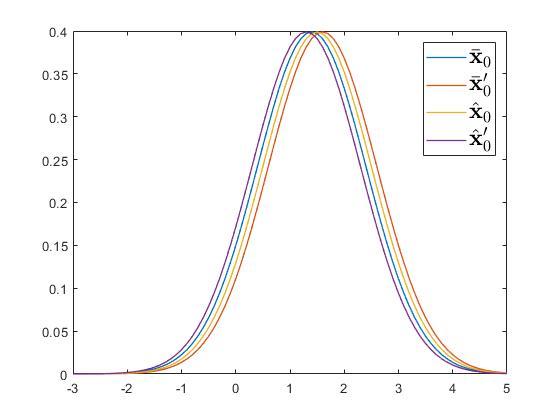
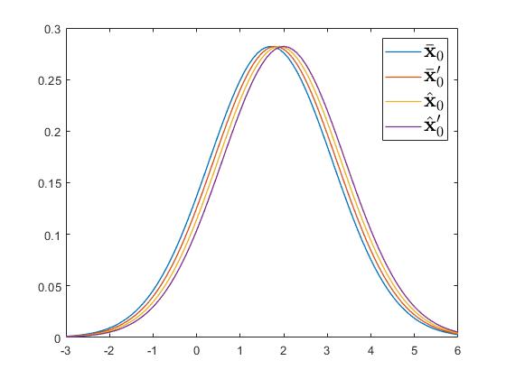
Regarding the differential privacy, we let be the eavesdropped output trajectory, and be a guess from the eavesdroppers. The system then denies this guess by stating that for example . To verify whether this deny is plausible, the eavesdroppers thus compute and with any value satisfying , and find . In this way, the system has gained plausible deniability measured by and . On the other hand, we randomly choose four adjacent initial values . The resulting distributions of under these initial values are presented in Figures 1 and 2. From Figures 1 and 2, it can be seen that the resulting probabilities of output trajectory at any set are similar. This thus can imply that the system in Case (b) preserves the differential privacy of initial values.
In view of the previous analysis for Cases (a) and (b), we can see that neither the intrinsic initial-value privacy implies the differential initial-value privacy, nor the differential initial-value privacy implies the intrinsic initial-value privacy. Therefore, both privacy metrics in Definitions 1 and 2 are mutually neither inclusive nor exclusive.
2.3 Related Works
Of relevance to our paper are recent works [15, 17, 16]. In [15], the considered linear dynamical systems take the form
where is a signal to be estimated, and the problem is to design a filter
| (7) |
with filter output , for the purpose of obtaining an optimal mean squared error between and , while preserving the differential privacy of system state trajectory , with the initial state considered in this paper as a particular case. Despite of this, we note that our framework can be extended to the scenario where are sensitive, which will be explicitly addressed in Remark 5. On the other hand, in [15], the eavesdropped information is a filter output trajectory , that is different from our paper where the eavesdroppers can directly measure system outputs. To address the desired privacy concerns, [15] studies the differential privacy of a composite mapping , the mapping and the mapping is defined over the filter dynamics (7). This is different mechanism compared to our mapping (4).
In [17] a cloud-based linear quadratic regulation problem is studied for systems of the form
where the outputs are transmitted to the cloud for an optimal control, having the form
The privacy issue of interest is to protect privacy of the state trajectory , against the eavesdroppers having access to the transmitted information consisting of by cyber attack. To address the state-trajectory privacy, [17] studies the differential privacy of the mapping . Therefore, again this is different mechanism compared to our mapping (4).
In [16], the authors consider a control system
where are injected input and measurement noise for privacy protection, and to achieve the desired control objective, the control input is designed as a form
| (8) |
The eavesdroppers having access to an output trajectory through cyber attack attempt to infer control inputs and initial values . In this setting, [16] studies the differential privacy of a mapping from to over the -dynamics. Compared to our mapping (4), the considered mapping in [16] is similar in the sense that both are established over the -dynamics, while is different in the sense that there are output trajectories and no control input in our mapping (4).
In addition to the previous distinctions, we note that this paper also studies privacy issues when an infinite number of output trajectories are eavesdropped, while it is absent in [15, 17, 16]. This extra study benefits us to understand whether the initial-value privacy can be preserved if the eavesdroppers have obtained a large number of output trajectories.
3 Initial-Value Privacy of General Linear Systems
In this section, both intrinsic and differential initial-value privacy of systems (1) are analyzed. We first present the following result on the equivalence of intrinsic initial-value privacy and unobservability.
Proposition 1
The system (1) preserves intrinsic initial-value privacy if and only if is not observable, i.e., .
Remark 3
Observability has been extensively studied in the fields of estimation [25] and feedback control [26]. In [16], for a linear control system the input observability is also explored to preserve differential privacy of control inputs and initial states. In Proposition 1, the intrinsic initial-value privacy and observability are bridged for linear systems (1).
Theorem 1
Suppose that are random variables according to . Then the dynamical system (1) preserves -differential privacy of initial state under -adjacency, with and , if
| (9) |
Remark 4
In Theorem 1, are assumed to admit Gaussian distributions. This renders the mapping (4) to be a Gaussian mechanism [15, 10], resulting in the -differential privacy. One may wonder if assuming Laplacian noise would lead to a stronger -differential privacy, as in [14]. However, we note that the resulting mapping (4) is not a Laplace mechanism, because there is no guarantee that is still Laplacian, even if are Laplacian variables.
Remark 5
Though only initial values of system (1) are treated as private information, we note that the results in Theorem 1 can be extended to the case that all states are sensitive. For dynamical systems (1), the outputs for all in contain the information of , rendering a mapping from and as
By combining all , together, one then can establish a mapping from the state trajectory to the output trajectory . For such a combined mapping, following the arguments in the proof of Theorem 1, one then can establish -differential privacy of the state trajectory with some and . In this way, our framework can be further applied to solve the problems in [15, 17], where the state trajectory is private information.
We note that given any covariance matrix , there always exist and , depending on the norm of extended observability matrix such that (9) is satisfied, yielding the -differential initial-value privacy. Thus, the -differential initial-value privacy and the intrinsic initial-value privacy are mutually independent, with the latter determined by the unobservability of systems (1), i.e., by Proposition 1. If the noise can be designed, then there always exists a sufficiently large covariance matrix such that (9) holds for any privacy budgets . To have a better view of this, we consider a particular case that and are i.i.d. random variables. The following corollary can be easily derived by verifying the condition (9).
Corollary 1
Suppose and , are i.i.d. random variables according to and . Then for any , , and all and , the dynamical system (1) preserves -differential privacy of initial state under -adjacency.
Remark 6
Though in Corollary 1 arbitrary -differential privacy can be achieved by choosing a sufficiently large , this doesn’t mean that the process noise does not contribute to the differential privacy. In fact, simple calculations following the proof of Theorem 1 can lead to a less restrictive condition as
from which it can be seen that also plays a role in achieving arbitrary differential privacy of initial values.
Remark 7
If the considered systems take a time-varying form
| (10) |
where the state and output matrices vary as evolves, it can be easily verified that the claims in Proposition 1 and Theorem 1 are still preserved by replacing the observability matrix and the extended observability matrix by their time-varying version .
4 Intrinsic Initial-Value Privacy of Networked Linear Systems
The system (1) can also be understood from a network system perspective, e.g.,[24]. Let be the -th entry of . If each is viewed as the dynamical state of a node, the matrix would indicate a graph of interactions among the nodes. If each entry of is viewed as the measurement of a sensor, then the matrix would indicate a graph of interactions between the nodes and the sensors.
In view of this, we consider a network consisting of network nodes and sensing nodes, leading to a network node set and a sensing node set 111To be distinguished with notations for nodes in the interaction graph , we use to denote the -th sensing node whose measurement is ., respectively. Define the interaction graph with edge set , and the sensing graph with edge set . Let and .
To this end, this section aims to study how topological effects affect the privacy analysis of the networked system (1) with being a configuration complying with the graphs , i.e., if for and for .
Remark 8
For the LTV systems (10), the corresponding network structure becomes time-varying, where matrix indicates a graph of interactions among the network nodes at time and matrix indicates a graph of interactions between the network and sensing nodes at time . Thus we define the time-varying interaction graph with edge set , and the sensing graph with edge set .
4.1 Intrinsic privacy of individual initial values
It is noted that in Definition 1 regarding intrinsic initial-value privacy, the initial state vector is considered as a whole, and we suppose that the eavesdroppers have no prior knowledge of any individual initial values. In the following, we present several definitions that refine the notion in Definition 1 to dynamical networked systems (1) by studying intrinsic privacy of individual initial values, i.e., , against eavesdroppers having knowledge of the whole sensor measurements (i.e., ) and initial values of some network nodes. For convenience, we term the set of nodes whose initial values are prior knowledge to eavesdroppers as a public disclosure set.
Definition 3
For any given configuration complying with graphs , take and let . The networked system (1) preserves intrinsic initial-value privacy of node w.r.t. public disclosure set if for any initial state , there exists an such that , for all , and
| (11) |
Remark 9
Remark 10
If the eavesdroppers have no prior knowledge of any node initial states, the above definition is also applicable with . In this case, according to Proposition 1, the notion of intrinsic initial-value privacy of node is related to state variable unobservability of state , that is a dual notion of state variable uncontrollability in [29].
Let and . Define . For convenience, we further let and , and be the -the column of matrix .
Theorem 2
Remark 11
Recalling (2), it can be seen that each initial state is multiplied by the -th column of the (extended) observability matrix. We term each -th column of the observability matrix as a “feature” vector of the corresponding node , and the columns corresponding to nodes in public set and unpublic set as public and unpublic “feature” vectors, respectively. Then, the equivalence of statements and demonstrates that the intrinsic initial-value privacy of node is preserved if and only if its “feature” vector can be expressed by a linear combination of the remainder unpublic “feature” vectors, i.e., the -th “feature” vector is encrypted by the remainder unpublic ones.
Remark 12
In Theorem 2, the equivalence of statements and demonstrates that the intrinsic initial-value privacy of node is preserved if and only if does not belong to the -extended observable subspace, denoted by .
Remark 13
It is worth noting that the verification of statement can be simplified as
-
c′).
.
This can be easily verified by using the following facts that
In view of this, we occasionally use c′) to replace c) in Theorem 2 in the sequel.
In Theorem 2, explicit rank conditions are proposed to determine whether the intrinsic initial-value privacy of individual nodes is preserved, with respect to any given public disclosure set . On the other hand, for a networked system, one may naturally ask what is the maximum allowable disclosure such that there always exists at least one node whose initial-value privacy is preserved. To address this issue, the network privacy index is introduced below.
Definition 4
The networked system (1) achieves level- network privacy, if for any public disclosure set with , there exists a node whose intrinsic initial-value privacy is preserved w.r.t. . The network privacy index of (1), denoted as , is defined as the maximal value of such that level- relative privacy is achieved.
Proposition 2
The network privacy index of networked system (1) is .
Remark 14
By Definition 4, the full initial value is not disclosed irrespective of which nodes are public. It is clear that a larger means a stronger privacy-preservation ability of the networked system (1). According to Proposition 2, this further implies that a networked system possesses a better privacy-preservation ability, if the dimension of its unobservable subspace (i.e., ) is higher.
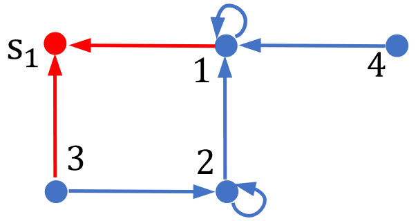
Example 2. We present an example to illustrate Theorem 2 and Proposition 2. Consider a networked system (1) with complying with the graphs in Fig. 3, consisting of 20 network nodes and 2 sensing nodes. Each edge of is assigned with the same weight 1.
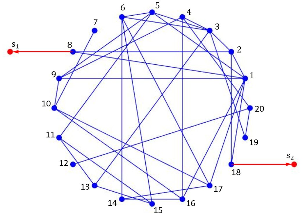
Firstly, suppose the eavesdroppers have no prior knowledge of initial values of any nodes, i.e., . We observe that . According to Proposition 2, this indicates that the network privacy index . Moreover, for all , there holds
According to Theorem 2, this indicates that the networked system preserves intrinsic initial-value privacy of all .
Let the public disclosure set . Taking into account the intrinsic initial-value privacy of individual nodes, we note that
for all . This verifies statement and thus indicates that the networked system preserves intrinsic initial-value privacy of all nodes , even if the initial states of nodes are public.
4.2 Generic intrinsic initial-value privacy
In the previous subsection, the intrinsic initial-value privacy of individual nodes w.r.t. the public disclosure set of networked systems (1) is studied, and a network privacy index is proposed to quantify the privacy of networked system (1). In the following, we turn to study the effect of network structure to the intrinsic privacy and the network privacy index. To be precise, we demonstrate that these properties are indeed generic, i.e., are fulfilled for almost all edge weights under any network structure .
Theorem 3
Let and . Then the intrinsic initial-value privacy of node w.r.t. is generically determined by the network topology. To be precise, exactly one of the following statements holds for any non-trivial network structure .
-
(i)
The intrinsic initial-value privacy of node is preserved generically, i.e., for almost all configurations complying with the network structure .
-
(ii)
The intrinsic initial-value privacy of node is lost generically, i.e., for almost all configurations complying with the network structure .
Theorem 3 demonstrates that given any network structure and , the intrinsic initial-value privacy of node is either preserved or lost generically. We note that if there exists a configuration complying with such that the intrinsic initial-value privacy of node is preserved (or lost), there is no guarantee that such property is preserved (or lost) generically. This is different from other common generic properties like structural controllability [34], for which if there exists a configuration such that a linear system is controllable, then it must be controllable for almost all configurations, i.e., structurally controllable. To have a better view of this, the following examples are formulated.
Example 3. Consider the intrinsic initial-value privacy of node 1 with complying with the network structure in Fig. 4. Let , and the system output trajectory is given by (2) with
It is clear that is full-rank for almost all configurations complying with Fig. 4. Thus, for any with , and thus hold for almost all configurations complying with Fig. 4. According to Definition 3, this indicates that the intrinsic initial-value privacy of node 1 is lost generically.
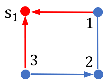
However, by letting the configuration be such that , simple calculations show that holds for any with and . According to Definition 3, this indicates that the intrinsic initial-value privacy of node 1 is preserved under the configuration satisfying .
Thus, even if there exists a configuration such that the intrinsic initial-value privacy of node is preserved, this property may still be lost generically. This validates the statement (i) of Theorem 3.
Example 4. Consider the intrinsic initial-value privacy of node 4 under the network structure in Fig. 5. Let , and the output trajectory is given by (2) with
with and . Simple calculations then can show that holds for any with and for , where ’s satisfy
| (12) |
It is clear that the above matrix equations (12) have a solution for almost all configurations complying with Fig. 5, which, by Definition 3, indicates that the intrinsic initial-value privacy of node 4 is preserved generically.
However, by letting the configuration be such that and , it can be seen that there exists no ’s such that the matrix equations (12) holds for any , and
with being some function of noise vectors . This immediately yields for all with . By Definition 3, this indicates that the intrinsic initial-value privacy of node 4 is lost under the configuration satisfying and .
Thus, even if there exists a configuration such that the intrinsic initial-value privacy of node is lost, such property may still be preserved generically. This is consistent with the statement (ii) of Theorem 3.
Denote the maximal rank of over the matrix pairs that comply with the network structure as . By Lemma 2 in Appendix E, it is noted that holds for almost all configurations complying with the network structure . We now present a practical verification approach of the intrinsic initial-value privacy of a node over the network structure .
Let the entries of and be generated independently and randomly according to the uniform distribution over the interval , and complying with the structure . We introduce the following three conditions:
-
()
.
-
()
with .
-
()
Denote as one realized sample from this randomization, from which we define the following event
We present the following result.
Theorem 4
The following statements hold.
-
(i)
If the event occurs, then we know with certainty (in the deterministic sense) that intrinsic initial-value privacy of node is preserved generically over the network structure .
-
(ii)
If intrinsic initial-value privacy of node is preserved generically, then must occur with probability one.
Theorem 4 indeed indicates a two-step approach to verify whether the intrinsic initial-value privacy of individual nodes is preserved generically. Given any set and node , the first step is to compute the maximal rank of . In practice, since holds for almost all configurations complying with the network structure , the value can be obtained by computing the maximal under a few independently and randomly generated configurations . The second step is to verify whether the event occurs under the independently and randomly generated configurations. If the event occurs, one then conclude that the intrinsic initial-value privacy of node is preserved generically. Otherwise, if the event does not occur, the intrinsic initial-value privacy of node is lost generically by Theorem 3.
Remark 15
When , according to Theorem 2, the generic intrinsic initial-value privacy of node indicates that the node state is unobservable for almost all configurations complying with , i.e., structurally unobservable, that is an extension of the dual notion to structural state variable controllability [29], and structural observability [30, 32].
Similar to Theorem 3, the network privacy index is also generically determined by the network structure .
Theorem 5
The network privacy index is generically determined by the network topology. Namely, for almost all configurations complying with the network structure , the network privacy index with given by the maximal rank of the observability matrix .
Remark 16
Remark 17
Example 5. Now an example is presented to illustrate Theorems 4-5. We consider a networked system (1) with complying with the graphs in Fig. 6, consisting of 12 network nodes and 2 sensing nodes.
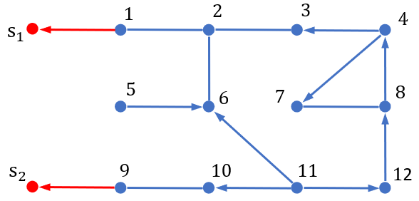
We choose five configurations with the entries generated independently and randomly according to the uniform distribution over the interval , and complying with the graph in Fig. 6. Under these configurations, we check the corresponding ranks of matrix , and find that the maximal rank is . According to Theorem 5, the network privacy index is , for almost all configurations complying with the graph in Fig. 6. Then, for each by fixing all edge weights as 1, it can be verified that
Using Theorem 4, this indicates that the network system preserves the intrinsic initial-value privacy of nodes for almost all configurations complying with the graph in Fig. 6.
Let the public disclosure set . Under the previously generated five configurations , we check the corresponding ranks of matrix , and find that the maximal rank is . Then fix all edge weights as 1 in Fig. 6, and we can obtain
By Theorem 4, this indicates that the network system preserves the intrinsic initial-value privacy of nodes for almost all configurations complying with the graph in Fig. 6, under the the public disclosure set .
Furthermore, let . Similarly, we check the corresponding ranks of matrix under the previously generated five configurations , and can find that , i.e., is full-column-rank for almost all configurations complying with the graph in Fig. 6. This implies that for all , there is no configuration such that
Thus, by Theorem 4 the intrinsic initial-value privacy of all nodes is generically lost.
Remark 18
We remark that for a large-scale system (1), it is generally difficult to determine the generic intrinsic initial-value privacy of individual nodes, due to the high computational complexity to compute the maximal rank of and verify the rank conditions in (C1)-(C3). A possible solution is to find topological conditions as in [34, 33]. However, the extension of ideas in [34, 33] to our settings is nontrivial, particularly in the presence of a public disclosure set . This will be further explored in future works.
5 Conclusions
In this paper, we have studied the intrinsic initial-value privacy and differential initial-value privacy of linear dynamical systems with random process and measurement noises. We proved that the intrinsic initial-value privacy is equivalent to unobservability, while the differential initial-value privacy can be achieved for a privacy budget depending on an extended observability matrix of the system and the covariance of the noises. Next, by regarding the considered linear system as a network system, we proposed necessary and sufficient conditions on the intrinsic initial-value privacy of individual nodes, in the presence of some nodes whose initial-value privacy is public. A quantitative network privacy index was also proposed using the largest number of arbitrary public nodes such that the whole initial values are not fully exposed. In addition, we showed that both the intrinsic initial-value privacy and the network privacy index are generically determined by the network structure. In future works, topological conditions (see e.g. [33, 34]) will be explored for generic intrinsic initial-value privacy of individual nodes, and the considered privacy metrics will be utilized to develop privacy-preservation approaches for linear dynamical systems.
Appendix A Proof of Proposition 1
Sufficiency. If , then and for all , we have
| (13) |
This, according to Definition 1, completes the sufficiency.
Necessity. To show the necessity part, the contradiction method is used. With the system (1) preserving intrinsic initial-value privacy, we suppose that . This implies that the mapping is invertible, i.e.,
It is clear that is identifiable from , i.e., the initial value of the system (1) is not private. This contradicts with the fact that the system (1) preserves intrinsic initial-value privacy. Therefore, it can be concluded that . This completes the proof.
Appendix B Proof of Theorem 1
Let be the process and measurement noise vectors, respectively for the -th implementation. Define and . Hence, with
As in [15], with the mapping defined in (4), for any and , we have
where is obtained by setting , is obtained by adding and subtracting the term , and setting , is obtained by choosing and setting with , and d) is derived by using the fact that . It is noted that
with .
Appendix C Proof of Theorem 2
Let be the -the column of matrix . Fundamental to the proof is the following technical lemma.
Lemma 1
Statement b) and c) in Theorem 2 are respectively equivalent to the following b†) and c†).
-
b†).
with .
-
c†).
.
Proof. We observe that with being full-column-rank, which yields
| (15) |
Namely,
Similarly, it can be verified that . Therefore, the statements b) and b†) are equivalent.
To show the equivalence between statements c) and c†), we observe that
This thus establishes the equivalence between statements and c†).
With the above lemma in mind, we now proceed to show and , which in turn will complete the proof.
. Given any node , we now proceed to show, if the initial-value privacy of node is preserved w.r.t. , . The contradiction method is used by supposing there exists no vector such that . This, in turn, implies there exists a vector such that and for all . Thus, given any initial condition , we have
which implies
It is clear that the initial condition of node is identifiable for system (1) w.r.t. , which contradicts with the fact that is private. Therefore, we conclude that , i.e., implies .
. Clearly, if
then there exists a vector such that . Given any and with , for , and , satisfying
we can obtain
Thus, given any nonzero , we let for all and for all , we have
| (16) |
with . This, according to Definition 3, proves .
. The equivalence between and can be easily inferred by using the facts that
Appendix D Proof of Proposition 2
The proof is completed if the following two statements are proved.
-
(i)
Given any with , there exists a node whose initial value is private.
-
(ii)
There exists a set with such that initial values of all nodes are identifiable.
Proof of part (i). Given any with , it is clear that the matrix is not full-column-rank, which indicates there exits an such that
According to Theorem 2, this yields that the initial value of node is private.
Proof of part (ii). Let and . Then, select , such that . Thus let . According to Theorem 2, it can be concluded that the initial values of all nodes are identifiable.
In summary of the previous analysis, we conclude that for system (1).
Appendix E Proof of Theorem 3
To ease the subsequent analysis, we collect all edge weights in a configuration vector with being the total number of edges in . In this way, all matrices are indeed functions of , and so is the resulting observability matrix .
Instrumental to the proof is the following lemma.
Lemma 2
There exists a such that
| (17) |
| (18) |
Proof. The proof of this lemma is to find the maximal value of with . Let , be such that
We run the following recursive algorithm from until is found.
Step : Check whether there exists such that . If so, using the fact that analytic functions that are not identically zero vanish only on a zero-measure set, we can conclude that holds for almost all . This, together with the fact that for all and all , indicates that (17) and (18) hold with . Otherwise, if for all , , we then proceed to Step .
If at the -th recursion of the above algorithm, we still cannot find a such that , we then can conclude that .
With this lemma, we now proceed to prove the theorem. Let be a set of configuration vector such that the intrinsic initial-value privacy of node is preserved for all and lost for all . It is clear that the proof is done if we show that either or is zero-measure. To prove it, we use the contradiction method, and assume that there exists a nonzero-measure set of configuration vector such that
-
()
the set is nonzero-measure, and
-
()
the intrinsic initial-value privacy of node is preserved only for under , and
-
()
the intrinsic initial-value privacy of node is lost for under .
Then, according to Theorem 2 and Remark 13, it can be inferred that
Let , be such that
By Lemma 2, there exists a nonzero-measure set such that the set is zero-measure, and for all , . Besides, it is clear that, for all
| (19) |
Since is nonzero-measure and is zero-measure, we have . Thus letting yields that and
This then implies with . Note that analytic functions that are not identically zero vanish only on a zero-measure set. This indicates that there is a nonzero-measure set of configuration vector such that
-
()
the set is zero-measure, and
-
()
the inequality holds for all .
Thus, for all , we have
which, together with (19), yields
for all . According to Theorem 2 and Remark 13, this implies that the intrinsic initial-value privacy of node is preserved for all configuration vector . Then by () and (), it immediately follows that , where the set is zero-measure. This indicates that is zero-measure, which contradicts with (), and thus completes the proof.
Appendix F Proof of Theorem 4
Recalling Theorem 2 and Remark 13, we can easily see that and are equivalent. Thus, the proof is done if the following two statements are proved.
-
()
If the condition () holds, then the intrinsic initial-value privacy of node is preserved generically.
-
()
If the intrinsic initial-value privacy of node is preserved generically, then the condition () holds for almost all configurations complying with .
Proof of (). By the condition (C1), there exists a such that
Following the notations in section E, we can obtain
with . Therefore, according to the standard arguments, there exists a nonzero-measure set such that the set is zero-measure, and the inequality holds for all . This yields
Therefore, with (18) we have
| (20) |
for all . Since for all with being zero-measure by Lemma 2, we thus obtain
| (21) |
for all . By Theorem 2 and Remark 13, this implies that the intrinsic initial-value privacy of node is preserved for all configurations . Note that is zero-measure, which proves ().
Proof of (). Suppose the intrinsic initial-value privacy of node is preserved generically. By Theorem 2 and Remark 13, this implies there exists a nonzero-measure set such that the set is zero-measure, and for all , (21) holds.
Recalling the fact that for all , we have
| (22) |
for all , where is zero-measure. This thus proves ().
Appendix G Proof of Theorem 5
Let , be such that
Since the maximal rank of is , it immediately follows that there exists a such that , and for all and . Note that analytic functions that are not identically zero vanish only on a zero-measure set. This indicates that there is a nonzero-measure set of configuration vector such that the set is zero-measure, and the inequality holds for all . Thus, we have holds for all . Recalling that is zero-measure, this indeed proves that holds for almost all .
With this in mind, we further combine with Proposition 2 and find that for all configuration , the resulting network privacy index . Recalling that is zero-measure, one then can conclude that the network privacy index holds for almost all configurations . This completes the proof.
References
- [1] J. P. Hespanha, P. Naghshtabrizi, Y. Xu, “A survey of recent results in networked control systems,” Proceedings of the IEEE, vol. 95, no. 1, pp. 138-162, 2007.
- [2] L. Atzori, A. Iera, and G. Morabito, “The internet of things: A survey,” Computer Networks, vol. 54, no. 15, pp. 2787-2805, 2010.
- [3] J. Gubbi, R. Buyya, S. Marusic, and M. Palaniswami, “Internet of Things (IoT): A vision, architectural elements, and future directions,” Future Generation Computer Systems, vol. 29, no. 7, pp. 1645-1660, 2013.
- [4] M. Kolhe, “Smart grid: Charting a new energy future: Research, development and demonstration,” The Electricity Journal, vol. 25, pp. 88–93, 2012.
- [5] P. Papadimitratos, A. D. La Fortelle, K. Evenssen, R. Brignolo and S. Cosenza, “Vehicular communication systems: Enabling technologies, applications, and future outlook on intelligent transportation,” IEEE Communications Magazine, vol. 47, no. 11, pp. 84-95, 2009.
- [6] J. Zhang, F. Wang, K. Wang, W. Lin, X. Xu and C. Chen, “Data-Driven Intelligent Transportation Systems: A Survey,” IEEE Transactions on Intelligent Transportation Systems, vol. 12, no. 4, pp. 1624-1639, 2011.
- [7] H. Sandberg, G. Dan, and R. Thobaben, “Differentially private state estimation in distribution networks with smart meters,” in Proc. 54th IEEE Conference on Decision and Control, pp. 4492-4498, 2015.
- [8] J. Ma, J. Qin, T. Salsbury, and P. Xu, “Demand reduction in building energy systems based on economic model predictive control,” Chemical Engineering Science, vol. 67, no.1, pp. 92-100, 2012.
- [9] C. Dwork, F. McSherry, K. Nissim, and A. Smith, “Calibrating noise to sensitivity in private data analysis,” in Proc. 3rd Theory of Cryptography Conference, pp. 265-284, 2006.
- [10] C. Dwork, K. Kenthapadi, F. McSherry, I. Mironov, and M. Naor, “Our data, ourselves: Privacy via distributed noise generation,” Annual International Conference on the Theory and Applications of Cryptographic Techniques, pp. 486-503, 2006.
- [11] A. Roth, “New algorithms for preserving differential privacy,” Ph.D., Carnegie Mellon Univ., Pittsburgh, PA, USA, 2010.
- [12] Z. Huang, S. Mitra, and G. Dullerud, “Differentially private iterative synchronous consensus,” in Pro. 2012 ACM Workshop on Privacy in the Electronic Society, pp. 81–90, ACM, 2012.
- [13] S. Han, U. Topcu, and G. J. Pappas, “Differentially private distributed constrained optimization,” IEEE Transactions on Automatic Control, vol. 62, no. 1, pp. 50–64, 2017.
- [14] E. Nozari, P. Tallapragada, and J. Cortes, “Differentially private distributed convex optimization via functional perturbation,” IEEE Transactions on Control of Network Systems, vol. 5, no. 1, pp. 395-408, 2018.
- [15] J. Le Ny and G. J. Pappas, “Differentially private filtering,” IEEE Transactions on Automatic Control, vol. 59, no. 2, pp. 341–354, 2014.
- [16] Y. Kawano and M. Cao, “Design of privacy-preserving dynamic controllers,” IEEE Transactions on Automatic Control, DOI:10.1109/TAC.2020.2994030.
- [17] M. Hale, A. Jones, K.Leahy, “Privacy in feedback: The differentially private LQG,” in Pro. IEEE American Control Conference, pp. 3386-3391, 2018.
- [18] S. Han and G. J. Pappas, “Privacy in control and dynamical systems,” Annual Review of Control, Robotics, and Autonomous Systems, vol.1, pp. 309-332, 2018.
- [19] J. Cortes, G. E. Dullerud, S. Han, J. Le Ny, S. Mitra, and G. J. Pappas, “Differential Privacy in control and network systems,” in Pro. 55th IEEE Conference on Decision and Control, pp. 4252-4272, 2016.
- [20] Y. Mo and R. M. Murray, “Privacy preserving average consensus,” IEEE Transactions on Automatic Control, vol. 62, no. 2, pp. 753-765, 2017.
- [21] F. Farokhi, and H. Sandberg, “Ensuring privacy with constrained additive noise by minimizing Fisher information,” Automatica, vol. 99, pp.275-288, 2019.
- [22] Y. Xu, W. Liu, and J. Gong, “Stable multi-agent-based load shedding algorithm for power systems,” IEEE Transactions on Power Systems, vol. 26, no. 4, pp. 2006-2014, 2011.
- [23] L. Wang, I. Manchester, J. Trumpf, and G. Shi, “Differential Observability for Initial-Value Privacy of Linear Dynamical Systems,” in Proc. 59th IEEE Conference on Decision and Control (CDC), 2020.
- [24] M. Mesbahi, M. Egerstedt. Graph Theoretic Methods in Multiagent Networks. Princeton University Press, 2010.
- [25] K. A. Clanents, G. R. Krutnpholz, P. W. Davis, “Power system state estimation with measurement deficiency: An observability/measurement placement algorithm,” IEEE Transactions on Power Apparatus and Systems, vol.7, pp. 2012-2020, 1983.
- [26] E. D. Sontag, Mathematical Control Theory, Texts in Applied Mathematics, 1998.
- [27] C. Dwork, A. Roth. The Algorithmic Foundations of Differential Privacy. Foundations and Trends in Theoretical Computer Science, 2014.
- [28] F. Pasqualetti, F. Dorfler, and F. Bullo, “Control-theoretic methods for cyberphysical security: Geometric principles for optimal cross-layer resilient control systems” IEEE Control Systems Magazin, vol. 35, no. 1, pp. 110-127, 2015
- [29] L. Blackhall, and D. Hill, “On the structural controllability of networks of linear systems,” in Proc. 2nd IFAC Workshop on Distributed Estimation and Control in Networked Systems, pp.245-250, 2010.
- [30] J. L. Willems, “Structural controllability and observability,” Systems & Control Letters, vol.8, pp.5-12, 1986.
- [31] S. Hosoe, “Determination of generic dimensions of controllable subspaces and its application,” IEEE Transactions on Automatic Control, vol.25, no.6, pp.1192-1196, 1981.
- [32] B. Y. Chang, R. D. Shachter, “Structural controllability and observability in influence diagrams,” in Proc. 8th Conference on Uncertaity in Artificial Intelligence, Standford University, pp. 25-32, 1992.
- [33] J. M. Hendrickx, M. Gevers, and A. S. Bazanella, “Identifiability of dynamical networks with partial node measurements,” IEEE Transactions on Automatic Control, vol. 64, no. 6, pp. 2240–2253, 2019.
- [34] C. T. Lin, “Structural controllability,” IEEE Transactions on Automatic Control, vol. 19, no. 3, pp. 201-208, 1974.