Initial Value Problem of the Whitham Equations for the Camassa-Holm Equation

Tamara Grava grava@sissa.it V. U. Pierce virgilpierce@gmail.com Fei-Ran Tian tian@math.ohio-state.edu SISSA, Via Beirut 2-4, 34014 Trieste, Italy Department of Mathematics, Ohio State University, 231 W. 18th Avenue, Columbus, OH 43210

Abstract

We study the Whitham equations for the Camassa-Holm equation. The equations are neither strictly hyperbolic nor genuinely nonlinear. We are interested in the initial value problem of the Whitham equations. When the initial values are given by a step function, the Whitham solution is self-similar. When the initial values are given by a smooth function, the Whitham solution exists within a cusp in the $x$ - $t$ plane. On the boundary of the cusp, the Whitham solution matches the Burgers solution, which exists outside the cusp.

keywords:

Camassa-Holm equation , Whitham equations , Non-strictly hyperbolic , Hodograph transform

PACS:

02.30.Ik , 02.30.Jr

, , and

1 Introduction

The Camassa-Holm equation

u_{t}+(3u+2\nu)u_{x}-\epsilon^{2}(u_{xxt}+2u_{x}u_{xx}+uu_{xxx})=0\ ,\quad u(x,0;\epsilon)=u_{0}(x)

(1)

describes waves in shallow water when surface tension is present [2]. Here, $\nu$ is a constant parameter. The solution of the initial value problem (1) will develop singularities in a finite time if and only if some portion of the positive part of the initial “momentum” density $u_{0}(x)-\epsilon^{2}u_{0}^{\prime\prime}(x)+\nu$ lies to the left of some portion of its negative part [10]. In particular, a unique global solution is guarenteed if $u_{0}(x)-\epsilon^{2}u_{0}^{\prime\prime}(x)+\nu$ does not change its sign. These are the non-breaking initial data that we are interested in throughout this paper.

Although the zero dispersion limit of equation (1) has not been established, some of its modulation equations (i.e., Whitham equations) have been derived. The zero phase Whitham equation is

u_{t}+(3u+2\nu)u_{x}=0\ ,\quad u(x,0)=u_{0}(x)\ ,

(2)

which can be obtained from (1) by formally setting $\epsilon=0$ .

The single phase Whitham equations have been found in [1] and they can be written in the Riemann invariant form

u_{ix}+\lambda_{i}(u_{1},u_{2},u_{3})u_{ix}=0\quad\mbox{for}-\nu<u_{3}<u_{2}<u_{1}\ ,

(3)

where

\lambda_{i}(u_{1},u_{2},u_{3})=u_{1}+u_{2}+u_{3}+2\nu-{I\over\partial_{u_{i}}I}\ ,

(4)

and

I(u_{1},u_{2},u_{3})=\int_{u_{3}}^{u_{2}}{\eta+\nu\over\sqrt{(\eta+\nu)(u_{1}-\eta)(u_{2}-\eta)(\eta-u_{3})}}\ d\eta\ .

The constraint $-\nu<u_{3}<u_{2}<u_{1}$ is consistent with the non-breaking initial data mentioned in the first paragraph of this section. The integral $I$ can be rewritten as a contour integral. Hence, it satisfies the Euler-Poisson-Darboux equations

2(u_{i}-u_{j}){\partial^{2}I\over\partial u_{i}\partial u_{j}}={\partial I\over\partial u_{i}}-{\partial I\over\partial u_{j}}\ ,\quad i,j=1,2,3

(5)

since the integrand does so for each $\eta\neq u_{i}$ . The Hamiltonian structure of the single phase Whitham equations for the Camassa-Holm equation was also obtained in [1] in terms of Abelian integrals. The higher phase Whitham equations can also be derived using this structure.

In this paper we will study the evolution of the Whitham solution from the zero phase to the single phase.

This problem is similar to that of the zero dispersion limit of the KdV equation [7, 8, 17]

u_{t}+6uu_{x}+\epsilon^{2}u_{xxx}=0\ ,\quad u(x,0;\epsilon)=u_{0}(x)\ .

(6)

It is known that the zero phase Whitham equation for the KdV equation is

u_{t}+6uu_{x}=0\ ,

(7)

which is equivalent to (2) for the Camassa-Holm equation. The single phase Whitham equations for the KdV equation are [3, 4, 18]

u_{ix}+\mu_{i}(u_{1},u_{2},u_{3})u_{ix}=0\ ,\quad\mbox{for}\quad u_{3}<u_{2}<u_{1}\ ,

(8)

where

\mu_{i}(u_{1},u_{2},u_{3})=2[u_{1}+u_{2}+u_{3}-{\tilde{I}\over\partial_{u_{i}}\tilde{I}}]\ ,

and

\tilde{I}(u_{1},u_{2},u_{3})=\int_{u_{3}}^{u_{2}}{1\over\sqrt{(u_{1}-\eta)(u_{2}-\eta)(\eta-u_{3})}}\ d\eta\ .

These equations are also similar to (3) and (4) for the Camassa-Holm equation.

In the KdV case, the evolution from the zero phase to the single phase has been studied in [14]. There, the Euler-Poisson-Darboux equations (5) have played an important role. The same equations have also played a crucial role in the study of the transition from the single phase to the double phase in [5].

Although both the Camassa-Holm equation (1) and the KdV equation (6) are dispersive approximations to the Burgers equation (2) or (7), there are significant differences in the limiting dynamics. The biggest difference is that the Whitham equations (3) for the former equation are non-strictly hyperbolic (cf. (36)) while the Whitham equations (8) for the latter equation are strictly hyperbolic [9]. Non-Strictly hyperbolic Whitham equations have also been found in the higher order KdV flows [11, 12, 13] and the higher order defocusing NLS flows [6]. Self-similar solutions of these Whitham equations have been constructed. They are remarkably different from the self-similar solutions of the KdV-Whitham equations [11, 12] or the NLS-Whitham equations [6], both of which are strictly hyperbolic.

In this paper, we will modify the method of paper [14] so that it can be used to solve the non-strictly hyperbolic Whitham equations (3) when the initial function is a smooth function. We will then study the evolution from the zero phase to the single phase for smooth initial data. When the initial function is a step-like function, we will use the method of paper [6, 11, 12] to study the same evolution.

The organization of the paper is as follows. In Section 2, we will introduce an initial value problem which describes the evolution of phases. We will also discuss how to use the hodograph transform to solve non-strictly hyperbolic Whitham equations. In Section 3, we will study the properties of the eigenspeeds of the single phase Whitham equations. We will study the initial value problem when the initial function $u_{0}(x)$ is a step-like function in Section 4 and when $u_{0}(x)$ is a smooth decreasing function in Section 5.

2 An Initial Value Problem

We describe the initial value problem for the Burgers equation (2) and Whitham equations (3) as follows (see Figure 1.). Consider a horizontal motion of the initial curve $u=u_{0}(x)$ . At the beginning, the curve evolves according to the Burgers equation (2). The Burgers solution breaks down in a finite time. Immediately after the breaking, the curve develops three branches. Denote these three branches by $u_{1}$ , $u_{2}$ , and $u_{3}$ . Their motion is governed by the Whitham equations (3). As time goes on, the Whitham solution may develop singularities and more branches are created. However, our focus is on the evolution of the solution of the Whitham equations from the one branch regime to the three branch regime.

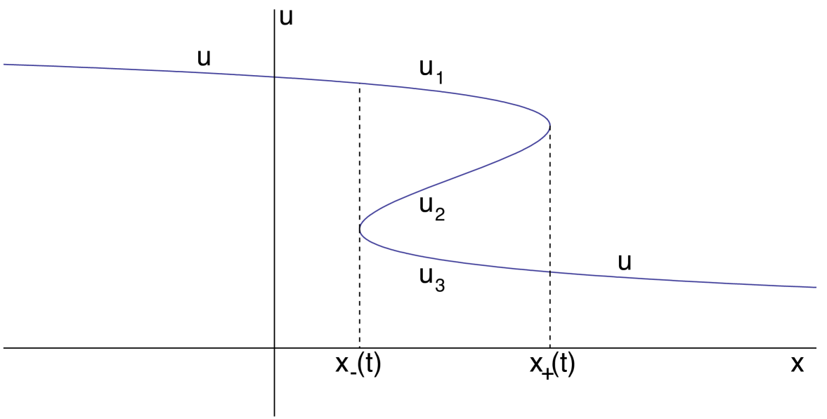
Refer to caption — Figure 1: Profile of the Burgers and Whitham solutions. The Burgers solution $u$ of (2) lives in the single value regions while the Whitham solution $u_{1}$ , $u_{2}$ and $u_{3}$ of (3) reside in the multiple value region.

The Burgers solution $u$ of (2) and the Whitham solution $u_{1}$ , $u_{2}$ , $u_{3}$ of (3) must match on the trailing edge $x=x_{-}(t)$ and leading edge $x=x_{+}(t)$ . We see from Figure 1 that

\displaystyle\left\{\begin{array}[]{c}u_{1}=u\\ u_{2}=u_{3}\end{array}\right.

(11)

must be imposed on the trailing edge, and that

\displaystyle\left\{\begin{array}[]{c}u_{1}=u_{2}\\ u_{3}=u\end{array}\right.

(14)

must be satisfied on the leading edge.

In this paper, we consider the initial function $u_{0}(x)$ that is monotone. Since the Burgers solution will not develop any shock if $u_{0}(x)$ is an increasing function, we will focus on decreasing initial functions. Denoting the inverse function of $u_{0}(x)$ by $f(u)$ , the Burger equation (2) can be solved using the method of characteristics; its solution is given implicitly by a hodograph transform,

x=(3u+2\nu)t+f(u)\ .

(15)

The solution method (15) has been generalized to solve the first order quasilinear hyperbolic equations which can be written in Riemann invariant form and which are strictly hyperbolic

{\partial u_{i}\over\partial t}+s_{i}(u_{1},\cdots,u_{n}){\partial u_{i}\over\partial x}=0\ ,\quad i=1,2,\cdots,n.

(16)

The strict hyperbolicity means that the wave propagation speeds $s_{i}$ ’s do not coincide.

We include Tsarev’s theorem for completeness [14, 16].

Theorem 1

If $w_{i}(u_{1},u_{2},\cdots,u_{n})$ ’s solve the linear equations

{\partial w_{i}\over\partial u_{j}}=A_{ij}(w_{i}-w_{j})

(17)

with

A_{ij}={{\partial s_{j}\over\partial u_{j}}\over s_{i}-s_{j}}

(18)

for $i,j=1,2,\cdots,n$ and $i\neq j$ , then the solution $(u_{1}(x,t),\cdots,u_{n}(x,t))$ of the hodograph transform,

x=s_{i}(u_{1},u_{2},\cdots,u_{n})t+w_{i}(u_{1},u_{2},\cdots,u_{n})

(19)

satisfies equations (16). Conversely, any solution $(u_{1}(x,t),\cdots,u_{n}(x,t))$ of equations (16) can be obtained in this way in the neighborhood of $(x_{0},t_{0})$ at which $u_{ix}$ are not all vanishing.

The strict hyperbolicity, i.e., $s_{i}\neq s_{j}$ for $i\neq j$ , of (16) is assumed to ensure that $A_{ij}$ ’s of (18) are not singular.

The result is classical when $n=2$ .

The validity of this theorem hinges on two factors. First, the linear equations (17) must have solutions. Secondly, the hodograph transform (19) must not be degenerate, i.e., it can be solved for $u_{i}$ ’s as functions of $x$ and $t$ . One interesting observation is that the Jacobian matrix of (19) is always diagonal on the solution $(u_{1}(x,t),\cdots,u_{n}(x,t))$ .

Corollary 2

At the solution $(u_{1}(x,t),\cdots,u_{n}(x,t))$ of $x=s_{i}(u_{1},u_{2},\cdot,u_{n})t+w_{i}(u_{1},u_{2},\cdots,u_{n})$ , $i=1,2,\cdots,n$ , the partial derivatives

\frac{\partial(s_{i}t+w_{i})}{\partial u_{j}}=0

for $i\neq j$ .

Proof.

$\displaystyle\frac{\partial(s_{i}t+w_{i})}{\partial u_{j}}$	$\displaystyle=$	$\displaystyle\frac{\partial s_{i}}{\partial u_{j}}t+\frac{\partial w_{i}}{\partial u_{j}}$
	$\displaystyle=$	$\displaystyle A_{ij}[(s_{i}t+w_{i})-(s_{j}t+w_{j})]$
	$\displaystyle=$	$\displaystyle 0\ .$

∎

Another aspect of Theorem 1 is that it is a local result. Solutions produced by the hodograph transform are, in general, local in nature. However, global solutions can still be obtained if the conditions of the theorem are satisfied globally [5, 14].

The Whitham equations (3) will be shown to be non-strictly hyperbolic, i.e., $\lambda_{i}$ ’s coincide at some points $(u_{1},u_{2},u_{3})$ where $0<u_{3}+\nu<u_{2}+\nu<u_{1}+\nu$ . However, Theorem 1 can still be applied to equations (3) since the functions $A_{ij}$ ’s of (18) are still non-singular for the Whitham equations (3), even at the points of non-strict hyperbolicity.

Lemma 3

B_{ij}:={{\partial\lambda_{i}\over\partial u_{j}}\over\lambda_{i}-\lambda_{j}}={1\over 2}{(\lambda_{i}-\gamma)-2(u_{i}-u_{j})\over(\lambda_{j}-\gamma)(u_{i}-u_{j})}\ ,\quad i\neq j\,,

where $\gamma=u_{1}+u_{2}+u_{3}+2\nu$ .

Proof.

By (4), we calculate

	$\displaystyle\lambda_{i}-\lambda_{j}$	$\displaystyle=$	$\displaystyle I{\partial_{u_{i}}I-\partial_{u_{j}}I\over(\partial_{u_{i}}I)(\partial_{u_{j}}I)}=2I{(u_{i}-u_{j})\partial_{u_{i}u_{j}}^{2}I\over(\partial_{u_{i}}I)(\partial_{u_{j}}I)}\ ,$
	$\displaystyle{\partial\lambda_{i}\over\partial u_{j}}$	$\displaystyle=$	$\displaystyle{2(u_{i}-u_{j})\partial_{u_{i}u_{j}}^{2}I\over\partial_{u_{i}}I}+{I\partial_{u_{i}u_{j}}^{2}I\over(\partial_{u_{i}}I)^{2}}\ ,$

where we have used (5). Hence, we get

	$\displaystyle B_{ij}$	$\displaystyle=$	$\displaystyle{2(u_{i}-u_{j})+{I\over\partial_{u_{i}}I}\over{2I\over\partial_{u_{j}}I}(u_{i}-u_{j})}$
		$\displaystyle=$	$\displaystyle{1\over 2}{(\lambda_{i}-\gamma)-2(u_{i}-u_{j})\over(\lambda_{j}-\gamma)(u_{i}-u_{j})}\ ,$

where we have used (4) to express $I/\partial_{u_{i}}I$ . ∎

3 The Single Phase Whitham Equations

In this section, we will summarize some of the properties of the speeds $\lambda_{i}$ ’s of (4) for later use.

Function $I$ of (4) is a complete elliptic integral; indeed,

I(u_{1},u_{2},u_{3})={2(u_{3}+\nu)\Pi(\rho,s)\over\sqrt{(u_{1}-u_{3})(u_{2}+\nu)}}\ ,

(20)

where $\Pi(\rho,s)$ is the complete integral of third kind, and

\rho={u_{2}-u_{3}\over u_{2}+\nu}\ ,\quad s=\frac{(u_{2}-u_{3})(u_{1}+\nu)}{(u_{1}-u_{3})(u_{2}+\nu)}\ .

(21)

Properties of complete elliptic integrals of the first, second and third kind are listed in Appendix A.

Using the well known derivative formulae (99) and (100), one is able to rewrite $\lambda_{i}$ of (4) as [1]

$\displaystyle\lambda_{1}(u_{1},u_{2},u_{3})$	$\displaystyle=$	$\displaystyle u_{1}+u_{2}+u_{3}+2\nu+2(u_{1}-u_{2})\frac{(u_{3}+\nu)\Pi(\rho,s)}{(u_{2}+\nu)E(s)}\ ,$
$\displaystyle\lambda_{2}(u_{1},u_{2},u_{3})$	$\displaystyle=$	$\displaystyle u_{1}+u_{2}+u_{3}+2\nu+2(u_{3}-u_{2})\frac{(1-s)\Pi(\rho,s)}{E(s)-(1-s)K(s)}\ ,$	(22)
$\displaystyle\lambda_{3}(u_{1},u_{2},u_{3})$	$\displaystyle=$	$\displaystyle u_{1}+u_{2}+u_{3}+2\nu+2(u_{2}-u_{3})\frac{(u_{3}+\nu)\Pi(\rho,s)}{(u_{2}+\nu)[E(s)-K(s)]}\ .$

Here $K(s)$ and $E(s)$ are complete elliptic integrals of the first and second kind.

Using inequalities (105), we obtain

$\displaystyle\lambda_{1}-(u_{1}+u_{2}+u_{3}+2\nu)$	$\displaystyle>$	$\displaystyle 0\ ,$	(23)
$\displaystyle\lambda_{2}-(u_{1}+u_{2}+u_{3}+2\nu)$	$\displaystyle<$	$\displaystyle 0\ ,$	(24)
$\displaystyle\lambda_{3}-(u_{1}+u_{2}+u_{3}+2\nu)$	$\displaystyle<$	$\displaystyle 0\ ,$	(25)

for $u_{1}>u_{2}>u_{3}>-\nu$ . In view of (101-104) and (106-107), we find that $\lambda_{1}$ , $\lambda_{2}$ and $\lambda_{3}$ have behavior

(1) At $u_{2}$ = $u_{3}$ ,

\begin{array}[]{ll}\lambda_{1}(u_{1},u_{2},u_{3})=3u_{1}+2\nu\ ,\\ \lambda_{2}(u_{1},u_{2},u_{3})=\lambda_{3}(u_{1},u_{2},u_{3})=u_{1}+2u_{3}+2\nu-{4(u_{3}+\nu)(u_{1}-u_{3})\over u_{1}+\nu}\ .\end{array}

(26)

(2) At $u_{1}$ = $u_{2}$ ,

\begin{array}[]{ll}\lambda_{1}(u_{1},u_{2},u_{3})=\lambda_{2}(u_{1},u_{2},u_{3})=2u_{1}+u_{3}+2\nu\ ,\\ \lambda_{3}(u_{1},u_{2},u_{3})=3u_{3}+2\nu\ .\end{array}

(27)

Lemma 4

\frac{\partial\lambda_{3}}{\partial u_{3}}<\frac{3}{2}\frac{\lambda_{2}-\lambda_{3}}{u_{2}-u_{3}}<\frac{\partial\lambda_{2}}{\partial u_{2}}

for $0<u_{3}+\nu<u_{2}+\nu<u_{1}+\nu$ .

Proof.

Comparing formulae (4) and (22), we use (20) to obtain

{\partial I\over\partial u_{2}}={\sqrt{(u_{1}-u_{3})(u_{2}+\nu)}\over(u_{2}-u_{3})(u_{1}-u_{2})}\ [E-(1-s)K]\ .

(28)

Differentiating (4) for $\lambda_{2}$ and using (28) yields

$\displaystyle{\partial\lambda_{2}\over\partial u_{2}}$	$\displaystyle=$	$\displaystyle{I\partial^{2}_{u_{2}u_{2}}I\over(\partial_{u_{2}}I)^{2}}$	(29)
	$\displaystyle=$	$\displaystyle{(u_{3}+\nu)\Pi\over(u_{2}+\nu)[E-(1-s)K]^{2}}\times$
		$\displaystyle\times\left\{[s+{u_{2}-u_{3}\over u_{1}-u_{3}}-2{u_{1}-u_{2}\over u_{1}-u_{3}}][E-(1-s)K]+s(1-s)K\right\}\ .$

Using formulae (22) for $\lambda_{2}$ and $\lambda_{3}$ , we obtain

\lambda_{2}(u_{1},u_{2},u_{3})-\lambda_{3}(u_{1},u_{2},u_{3})={2(u_{2}-u_{3})(u_{3}+\nu)\Pi M(u_{1},u_{2},u_{3})\over(u_{2}+\nu)(K-E)[E-(1-s)K]}\ ,

(30)

where

M(u_{1},u_{2},u_{3})=[1+{u_{1}-u_{2}\over u_{1}-u_{3}}]E-[{u_{1}-u_{2}\over u_{1}-u_{3}}+(1-s)]K\ .

(31)

We then obtain from (29) and (30) that

	$\displaystyle{\partial\lambda_{2}\over\partial u_{2}}-{3\over 2}\ {\lambda_{2}-\lambda_{3}\over u_{2}-u_{3}}$	$\displaystyle=-{(u_{3}+\nu)(4-3s)\Pi E^{2}\over(u_{2}+\nu)[K-E][E-(1-s)K]^{2}}\left\{(1-s)({K\over E})^{2}\right.$
		$\displaystyle\phantom{=}\left.\quad-2({K\over E})+{4+s\over 4-3s}\right\}>0\ ,$

where the inequality follows from the negativity of the function in the bracket (c.f. (4.18) of [14]). This proves part of the lemma. The other part can be shown in the same way.

∎

We conclude this section with a few calculations. We use (97) and (98) to calculate the derivative of (31)

$\displaystyle{\partial M(u_{1},u_{2},u_{3})\over\partial u_{2}}$	$\displaystyle=$	$\displaystyle{1\over 2(u_{1}-u_{3})}\ \{[2+{(u_{1}+\nu)(u_{3}+\nu)\over(u_{2}+\nu)^{2}}]K$	(32)
		$\displaystyle\phantom{{1\over 2(u_{1}-u_{3})}\ \{}-[2+{u_{1}+\nu\over u_{2}+\nu}]E\}\ ,$	(32)
$\displaystyle{\partial^{2}M(u_{1},u_{2},u_{3})\over\partial u_{2}^{2}}$	$\displaystyle=$	$\displaystyle{(u_{1}+\nu)[4(u_{1}+\nu)-2(u_{2}+\nu)+(u_{3}+\nu)]E\over 4(u_{1}-u_{3})(u_{1}-u_{2})(u_{2}+\nu)^{2}}\ .$	(33)

Finally, we use the expansions (101-102) for $K$ and $E$ to obtain

$\displaystyle M(u_{1},u_{2},u_{3})$	$\displaystyle=$	$\displaystyle{\pi\over 2}\left\{{(u_{2}-u_{3})s\over 2(u_{1}-u_{3})}+{1\over 16}\ (1-{3(u_{1}-u_{2})\over u_{1}-u_{3}})s^{2}\right.$	(34)
		$\displaystyle\phantom{{\pi\over 2}}\left.\quad+{3\over 128}(1-{5(u_{1}-u_{2})\over u_{1}-u_{3}})s^{3}+O(s^{4})\right\}$
	$\displaystyle=$	$\displaystyle{\pi\over 2}\left\{[{u_{2}+\nu\over 2(u_{1}+\nu)}+{1\over 16}\ (1-{3(u_{1}-u_{2})\over u_{1}-u_{3}})]s^{2}\right.$
		$\displaystyle\phantom{{\pi\over 2}}\left.\quad+{3\over 128}(1-{5(u_{1}-u_{2})\over u_{1}-u_{3}})s^{3}+O(s^{4})\right\}\,,$

where we have used formula (21) for $s$ in the last equality.

4 Step-like Initial Data

In this section, we will consider the step-like initial data

u_{0}(x)=\left\{\begin{matrix}a&\quad x<0\\ b&\quad x>0\end{matrix}\right.\ ,\ \quad a\neq b

(35)

for equation (1). Since the solution of (2) will never develop a shock when $a\leq b$ , we will be interested only in the case $a>b$ . We classify the initial data (35) into two types:

•

(I) $a+\nu>4(b+\nu)$ ,
•

(II) $a+\nu\leq 4(b+\nu)\,.$

We will solve the initial value problem for the Whitham equations for these two types of initial data.

4.1 Type I: $a+\nu>4(b+\nu)$

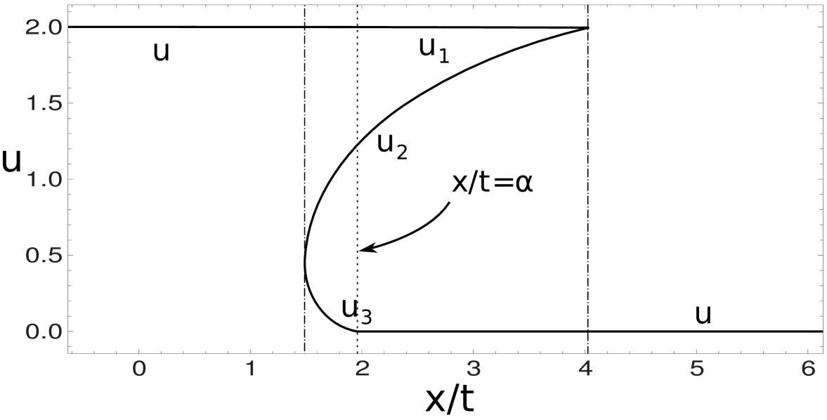
Theorem 5

(see Figure 2.) For the step-like initial data $u_{0}(x)$ of (35) with $0<b+\nu<(a+\nu)/4$ , the solution of the Whitham equations (3) is given by

u_{1}=a\ ,\quad x=\lambda_{2}(a,u_{2},u_{3})\ t\ ,\quad x=\lambda_{3}(a,u_{2},u_{3})\ t

(36)

for $(3a-\nu)/4<x/t\leq\alpha$ and by

u_{1}=a\ ,\quad x=\lambda_{2}(a,u_{2},b)\ t\ ,\quad u_{3}=b

(37)

for $\alpha t\leq x<(2a+b+2\nu)t$ , where $\alpha=\lambda_{2}(a,u^{*},b)$ and $u^{*}$ is the unique solution $u_{2}$ of $\lambda_{2}(a,u_{2},b)=\lambda_{3}(a,u_{2},b)$ in the interval $b<u_{2}<a$ . Outside the region $(3a-\nu)/4<x/t<2a+b+2\nu$ , the solution of the Burgers equation (2) is given by

u\equiv a\quad\mbox{$x/t\leq(3a-\nu)/4$}

(38)

and

u\equiv b\quad\mbox{$x/t\geq 2a+b+2\nu$}\ .

(39)

The boundaries $x/t=(3a-\nu)/4$ and $x/t=2a+b+2\nu$ are the trailing and leading edges, respectively, of the dispersive shock. They separate the solution into the region governed by the single phase Whitham equations and the region governed by the Burgers equation.

The proof of Theorem 5 is based on a series of lemmas.

We first show that the solutions defined by formulae (36) and (37) indeed satisfy the Whitham equations (3) [16].

Lemma 6

(i)

The functions $u_{1}$ , $u_{2}$ and $u_{3}$ determined by equations (36) give a solution of the Whitham equations (3) as long as $u_{2}$ and $u_{3}$ can be solved from (36) as functions of $x$ and $t$ .
(ii)

The functions $u_{1}$ , $u_{2}$ and $u_{3}$ determined by equations (37) give a solution of the Whitham equations (3) as long as $u_{2}$ can be solved from (37) as a function of $x$ and $t$ .

Proof.

(i) $u_{1}$ obviously satisfies the first equation of (3). To verify the second and third equations, we observe that

\frac{\partial\lambda_{2}}{\partial u_{3}}=\frac{\partial\lambda_{3}}{\partial u_{2}}=0

(40)

on the solution of (36). This follows from Lemma 3.

We then calculate the partial derivatives of the second equation of (36) with respect to $x$ and $t$ .

1=\frac{\partial\lambda_{2}}{\partial u_{2}}\ t(u_{2})_{x}\ ,\quad 0=\frac{\partial\lambda_{2}}{\partial u_{2}}\ t(u_{2})_{t}+\lambda_{2}\ ,

which give the second equation of (3).

The third equation of (3) can be verified in the same way.

(ii) The second part of Lemma 6 can easily be proved in a similar manner.

∎

We now determine the trailing edge. Eliminating $x$ and $t$ from the last two equations of (36) yields

\lambda_{2}(a,u_{2},u_{3})-\lambda_{3}(a,u_{2},u_{3})=0\ .

(41)

In view of formula (30), we replace (41) by

{M(a,u_{2},u_{3})\over s^{2}}=0\ .

(42)

Therefore, at the trailing edge where $u_{2}=u_{3}$ , i.e., $s=0$ , equation (42), in view of the expansion (34), becomes

{u_{3}+\nu\over 2(a+\nu)}+{1\over 16}\ [1-{3(a-u_{3})\over a-u_{3}}]=0\ ,

which gives $u_{2}=u_{3}=(a-3\nu)/4$ .

Lemma 7

Equation (42) has a unique solution satisfying $u_{2}=u_{3}$ . The solution is $u_{2}=u_{3}=(a-3\nu)/4$ . The rest of equations (36) at the trailing edge are $u_{1}=a$ and $x/t=\lambda_{2}(a,(a-3\nu)/4,(a-3\nu)/4)=(3a-\nu)/4$ .

Having located the trailing edge, we now solve equations (36) in the neighborhood of the trailing edge. We first consider equation (42). We use (34) to differentiate $M/s^{2}$ at the trailing edge $u_{1}=a$ , $u_{2}=u_{3}=(a-3\nu)/4$ , to find

{\partial\over\partial u_{2}}[{M\over s^{2}}]={\partial\over\partial u_{3}}[{M\over s^{2}}]={\pi\over 8(a+\nu)}\ ,

which shows that equation (42) or equivalently (41) can be inverted to give $u_{3}$ as a decreasing function of $u_{2}$

u_{3}=A(u_{2})

(43)

in a neighborhood of $u_{2}=u_{3}=(a-3\nu)/4$ .

We now extend the solution (43) of equation (41) in the region $a>u_{2}>(a-3\nu)/4>u_{3}>b$ as far as possible. We deduce from Lemma 4 that

{\partial\lambda_{2}\over\partial u_{2}}>0\ ,\quad{\partial\lambda_{3}\over\partial u_{3}}<0

(44)

on the solution of (41). Because of (40) and (44), solution (43) of equation (41) can be extended as long as $a>u_{2}>(a-3\nu)/4>u_{3}>0$ .

There are two possibilities: (i) $u_{2}$ touches $a$ before or simultaneously as $u_{3}$ reaches $b$ and (ii) $u_{3}$ touches $b$ before $u_{2}$ reaches $a$ .

It follows from (27) that

\lambda_{2}(a,a,u_{3})>\lambda_{3}(a,a,u_{3})\quad\mbox{for $b\leq u_{3}<a$}\ .

This shows that (i) is impossible. Hence, $u_{3}$ will touch $b$ before $u_{2}$ reaches $a$ . When this happens, equation (41) becomes

\lambda_{2}(a,u_{2},b)-\lambda_{3}(a,u_{2},b)=0\ .

(45)

Lemma 8

Equation (45) has a simple zero in the region $b<u_{2}<a$ , counting multiplicities. Denoting the zero by $u^{*}$ , then $\lambda_{2}(a,u_{2},b)-\lambda_{3}(a,u_{2},b)$ is positive for $u_{2}>u^{*}$ and negative for $u_{2}<u^{*}$ .

Proof. We use (30) and (33) to prove the lemma. In equation (30), $K-E$ and $E-(1-s)K$ are all positive for $0<s<1$ in view of (105). We claim that

M(a,u_{2},b)=0\quad\mbox{for $u_{2}=b$}\ ,\quad M(a,u_{2},b)<0\quad\mbox{for $u_{2}$ near $b$}\ ,

and

\quad M(a,u_{2},b)>0\quad\mbox{for $u_{2}=a$}\ .

The equality and the first inequality follow from expansion (34) and $a+\nu>4(b+\nu)$ . The second inequality is obtained by applying (103) and (104) to (31).

We conclude from the two inequalities that $M(a,u_{2},b)$ has a zero in $b<u_{2}<a$ . This zero is unique because $M(a,u_{2},b)$ , in view of (33), is a convex function of $u_{2}$ . This zero is exactly $u^{*}$ and the rest of the theorem is proven easily. ∎

Having solved equation (41) for $u_{3}$ as a decreasing function of $u_{2}$ for $(a-3\nu)/4\leq u_{2}\leq u^{*}$ , we turn to equations (36). Because of (40) and (44), the second equation of (36) gives $u_{2}$ as an increasing function of $x/t$ , for $(3a-\nu)/4\leq x/t\leq\alpha$ , where

\alpha=\lambda_{2}(a,u^{*},b).

Consequently, $u_{3}$ is a decreasing function of $x/t$ in the same interval.

Lemma 9

The last two equations of (36) can be inverted to give $u_{2}$ and $u_{3}$ as increasing and decreasing functions, respectively, of the self-similarity variable $x/t$ in the interval $(3a-\nu)\leq x/t\leq\alpha$ , where $\alpha=\lambda_{2}(a,u^{*},b)$ and $u^{*}$ is given in Lemma 8.

We now turn to equations (37). We want to solve the second equation when $x/t>\alpha$ or equivalently when $u_{2}>u^{*}$ . According to Lemma 8, $\lambda_{2}(a,u_{2},b)-\lambda_{3}(a,u_{2},b)>0$ for $u^{*}<u_{2}<a$ , which, by Lemma 4, shows that

{\partial\lambda_{2}(a,u_{2},b)\over\partial u_{2}}>0\ .

Hence, the second equation of (37) can be solved for $u_{2}$ as an increasing function of $x/t$ as long as $u^{*}<u_{2}<a$ . When $u_{2}$ reaches $a$ , we have

x/t=\lambda_{2}(a,a,b)=2a+b+2\nu\ ,

where we have used (27) in the last equality. We have therefore proved the following result.

Lemma 10

The second equation of (37) can be inverted to give $u_{2}$ as an increasing function of $x/t$ in the interval $\alpha\leq x/t\leq 2a+b+2\nu$ .

We are ready to conclude the proof of Theorem 5.

The Burgers solutions (38) and (39) are trivial.

According to Lemma 9, the last two equations of (36) determine $u_{2}$ and $u_{3}$ as functions of $x/t$ in the region $(3a-v)/4\leq x/t\leq\alpha$ . By the first part of Lemma 6, the resulting $u_{1}$ , $u_{2}$ and $u_{3}$ satisfy the Whitham equations (3). Furthermore, the boundary condition (11) is satisfied at the trailing edge $x/t=(3a-v)/4$ .

Similarly, by Lemma 10, the second equation of (37) determines $u_{2}$ as a function of $x/t$ in the region $\alpha\leq x/t\leq 2a+b+2\nu$ . It then follows from the second part of Lemma 6 that $u_{1}$ , $u_{2}$ and $u_{3}$ of (37) satisfy the Whitham equations (3). They also satisfy the boundary condition (14) at the leading edge $x=(2a+b+2\nu)t$ .

We have therefore completed the proof of Theorem 5.

A graph of the Whitham solution for the initial data (35) of type I is given in Figure 2. It is obtained by plotting the exact solutions of (36) and (37).

4.2 Type II: $a+\nu\leq 4(b+\nu)$

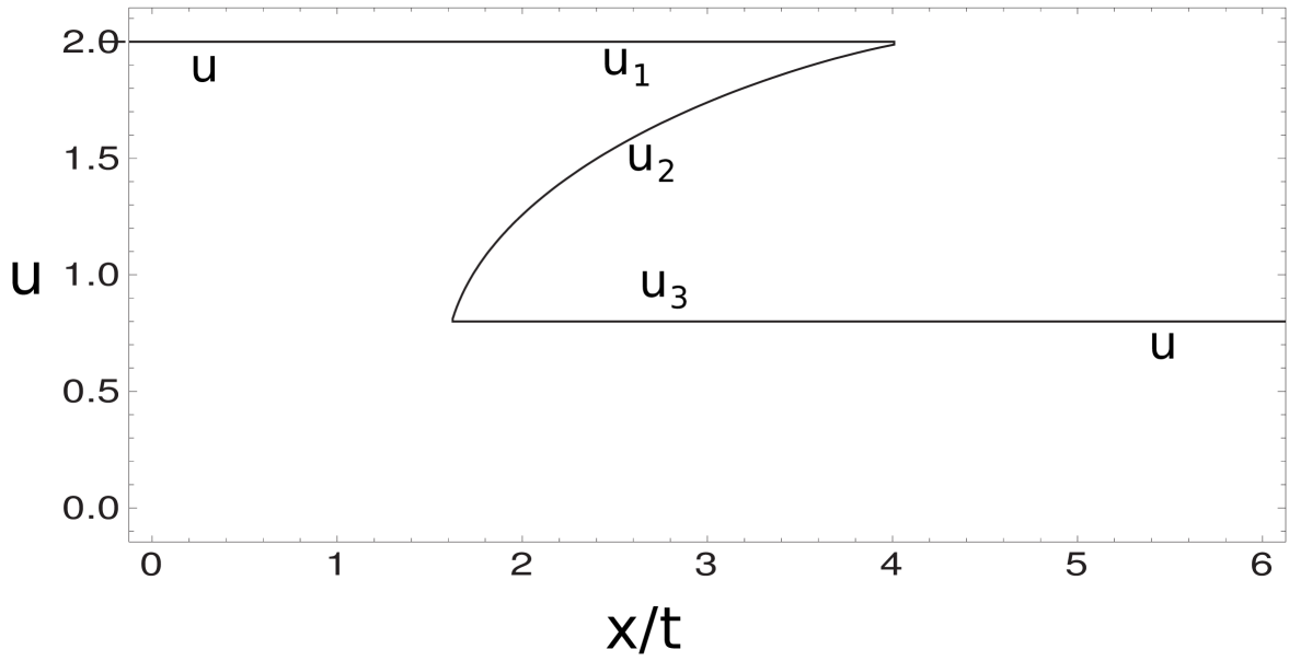
Theorem 11

(see Figure 3.) For the step-like initial data (35) with $0<(a+\nu)/4\leq b+\nu<a+\nu$ , the solution of the Whitham equations (3) is given by

u_{1}=a\ ,\quad x=\lambda_{2}(a,u_{2},b)\ t\ ,\quad u_{3}=b

(46)

for $\lambda_{2}(a,b,b)<x/t<\lambda_{2}(a,a,b)$ , where $\lambda_{2}(a,b,b)=a+2b+2\nu-4(a-b)(b+\nu)/(a+\nu)$ and $\lambda_{2}(a,a,b)=2a+b+2\nu$ . Outside this interval, the solution of (2) is given by

u\equiv a\quad\mbox{$x/t\leq\lambda_{2}(a,b,b)$}

and

u\equiv b\quad\mbox{$x/t\geq\lambda_{2}(a,a,b)$}\ .

Proof.

We will give a brief proof, since the arguments are, more or less, similar to those in the proof of Theorem 5.

It suffices to show that $\lambda_{2}(a,u_{2},b)$ is an increasing function of $u_{2}$ for $b<u_{2}<a$ . Using the inequality (105) to estimate the right hand side of (32), we obtain

	$\displaystyle{dM(a,u_{2},b)\over du_{2}}$	$\displaystyle>{(a+\nu)(u_{2}-b)E(s)\over 2(2-s)(a-b)^{2}(u_{2}+\nu)^{2}}\left\{2(u_{2}+\nu)+2(b+\nu)-\right.$
		$\displaystyle\phantom{>{(a+\nu)(u_{2}-b)E(s)\over 2(2-s)(a-b)^{2}(u_{2}+\nu)^{2}}}\left.-(a+\nu)\right\}>0$

for $b<u_{2}<a$ , where we have used $(a+\nu)/4\leq b+\nu$ in the second inequality. Since $M(a,u_{2},b)=0$ at $u_{2}=b$ in view of (34), this implies that $M(a,u_{2},b)>0$ for $b<u_{2}<a$ . It then follows from (30) that $\lambda_{2}(a,u_{2},b)-\lambda_{3}(a,u_{2},b)>0$ . By Lemma 4, we conclude that

{d\lambda_{2}(a,u_{2},b)\over du_{2}}>0

for $b<u_{2}<a$ .

∎

A graph of the Whitham solution for initial data (35) of type II is given in Figure 3. It is obtained by plotting the exact solution of (46).

5 Smooth Initial Data

In this section, we will study the initial value problem of the Whitham equations when the initial values are given by a smooth monotone function $u_{0}(x)$ . Since the Burgers solution of (2) will never develop a shock when $u_{0}(x)$ is an increasing function, we will be interested only in the case that $u_{0}(x)$ is a decreasing function.

We consider the initial function $u_{0}(x)$ which is a decreasing function and is bounded at $x=\pm\infty$

\lim_{x\rightarrow-\infty}u_{0}(x)=a\ ,\quad\lim_{x\rightarrow+\infty}u_{0}(x)=b\ .

(47)

By Theorem 1 and Lemma 3, we can use the hodograph transform,

x=\lambda_{i}(u_{1},u_{2},u_{3})t+w_{i}(u_{1},u_{2},u_{3})\ ,\quad i=1,2,3,

(48)

to solve the Whitham equations (3). Here, $w_{i}$ ’s satisfy a linear over-determined system of type (17)

\displaystyle{\partial w_{i}\over\partial u_{j}}=B_{ij}(w_{i}-w_{j})\ ,

(49)

where $B_{ij}$ ’s are given in Lemma 3.

The boundary conditions on $w_{i}$ ’s are obtained by observing that the hodograph solution (48) of the Whitham equations (3) must match the characteristic solution (15) of the Burgers equation (2) at the trailing and leading edges in the fashion of (11-14). By (26-27), $w_{i}$ ’s must satisfy the boundary conditions,

	$\displaystyle\left\{\begin{array}[]{l}w_{1}(u_{1},u_{1},u_{3})=w_{2}(u_{1},u_{1},u_{3}),\\ w_{3}(u_{1},u_{1},u_{3})=f(u_{3}),\end{array}\right.$		(52)
	$\displaystyle\left\{\begin{array}[]{l}w_{1}(u_{1},u_{3},u_{3})=f(u_{1}),\\ w_{2}(u_{1},u_{3},u_{3})=w_{3}(u_{1},u_{3},u_{3}),\end{array}\right.$		(55)

where $f(u)$ is the inverse of the initial function $u_{0}(x)$ .

Analogous to the KdV case [14, 15], equations (49) subject to boundary conditions (52-55) are related to a boundary value problem of a linear over-determined system of Euler-Poisson-Darboux type (cf. (5))

	$\displaystyle 2(u_{i}-u_{j})\frac{\partial^{2}q}{\partial{u_{i}}\partial{u_{j}}}$	$\displaystyle=$	$\displaystyle\frac{\partial q}{\partial u_{i}}-\frac{\partial q}{\partial u_{j}}\ ,\quad i,j=1,2,3,$		(56)
	$\displaystyle q(u,u,u)$	$\displaystyle=$	$\displaystyle f(u)\ ,$		(57)

for $i,j=1,2,3$ . The solution is unique and symmetric in $u_{1}$ , $u_{2},u_{3}$ . It is given explicitly by [14]

\displaystyle q(u_{1},u_{2},u_{3})=\frac{1}{2\sqrt{2}\pi}\int_{-1}^{1}\int_{-1}^{1}\frac{f({1+u\over 2}{1+v\over 2}u_{1}+{1+u\over 2}{1-v\over 2}u_{2}+{1-u\over 2}u_{3})}{\sqrt{(1-u)(1-v^{2})}}dudv\ .

(58)

Theorem 12

If $q(u_{1},u_{2},u_{3})$ is a solution of (56) and (57), then $w_{i}(u_{1},u_{2},u_{3})$ ’s given by

\displaystyle w_{i}\

\displaystyle=[\lambda_{i}(u_{1},u_{2},u_{3})-\gamma]\ {\partial q(u_{1},u_{2},u_{3})\over\partial u_{i}}+q(u_{1},u_{2},u_{3})\ ,

(59)

where $\gamma=u_{1}+u_{2}+u_{3}+2\nu$ , solve equations (49) and satisfy boundary conditions (52-55).

Proof.

By Lemma 3 and (56), we obtain

\displaystyle[\lambda_{j}-\gamma]\left[{\partial q\over\partial u_{i}}-{\partial q\over\partial u_{j}}\right]B_{ij}=\left({\partial q\over\partial u_{j}}-{\partial q\over\partial u_{i}}\right)+[\lambda_{i}-\gamma]{\partial^{2}q\over\partial u_{i}\partial u_{j}}\ .

(60)

Using (59), we calculate

	$\displaystyle{\partial w_{i}\over\partial u_{j}}$	$\displaystyle=$	$\displaystyle{\partial\lambda_{i}\over\partial u_{j}}{\partial q\over\partial u_{i}}+\left[\lambda_{i}-\gamma\right]{\partial^{2}q\over\partial u_{i}\partial u_{j}}+{\partial q\over\partial u_{j}}-{\partial q\over\partial u_{i}}\ ,$
	$\displaystyle w_{i}-w_{j}$	$\displaystyle=$	$\displaystyle\left[\lambda_{i}-\gamma\right][{\partial q\over\partial u_{i}}-{\partial q\over\partial u_{j}}]+\left[\lambda_{i}-\lambda_{j}\right]{\partial q\over\partial u_{i}}\ .$

Substituting these into (60), we find that $w_{i}$ ’s satisfy (49).

Finally, we shall check the boundary conditions (52-55). We only consider the leading edge, and the trailing edge can be handled in the same way.

Since $q(u_{1},u_{2},u_{3})$ is symmetric in $u_{1}$ , $u_{2}$ and $u_{3}$ , the first condition of (52) follows from (59) and (27).

For the second condition, it follows from (27) and (59) again that

w_{3}(u_{1},u_{1},u_{3})=2(u_{3}-u_{1}){\partial q\over\partial u_{3}}+q\ .

(61)

Differentiating this with respect to $u_{1}$ yields,

\displaystyle{\partial w_{3}\over\partial u_{1}}=-2{\partial q\over\partial u_{3}}+2(u_{3}-u_{1})[{\partial^{2}q\over\partial u_{1}\partial u_{3}}+{\partial^{2}q\over\partial u_{2}\partial u_{3}}]+{\partial q\over\partial u_{1}}+{\partial q\over\partial u_{2}}=0\ ,

where we have used (56) in the last equality. Since $w_{3}(u_{1},u_{1},u_{3})$ is independent of $u_{1}$ , we replace $u_{1}$ by $u_{3}$ in (61) and use (57) to obtain the second condition of (52).

∎

Theorem 12 has been reported in [1] in the case of $\nu=0$ .

In the rest of this section, we study the hodograph transform (48) with $w_{i}$ ’s given by (58) and (59). We shall show that the transform can be solved for $u_{1}$ , $u_{2}$ and $u_{3}$ as functions of $(x,t)$ within a cusp in the $x$ - $t$ plane.

Since $t_{b}=-[3\min\left(u^{\prime}_{0}(x)\right)]^{-1}$ is the breaking time of the Burgers solution of (2), the breaking is caused by an inflection point in the initial data. If $x_{0}$ is this inflection point, then $(x_{b},t_{b})$ is the breaking point on the evolving curve where $x_{b}=x_{0}+[3u_{0}(x_{0})+2\nu]t_{b}$ , and $t_{b}$ is the breaking time. Without loss of generality, we may assume $x_{b}=0$ , $t_{b}=0$ and denote $u_{0}(0)$ by $\hat{u}$ . The effect of these choices is that we are starting at the breaking time, and the evolving curve is about to turn over at the point $(0,\hat{u})$ in the $x$ - $u$ plane. It immediately follows that

f(\hat{u})=f^{\prime}(\hat{u})=f^{\prime\prime}(\hat{u})=0\ ,

(62)

where $x=f(u)$ is the inverse function of the decreasing initial data $u=u_{0}(x)$ . On the assumption that $x=f(u)$ has only one inflection point, it follows from the monotonicity of the function $f(u)$ that

f^{\prime\prime}(u)=\left\{\begin{array}[]{ll}<0&\quad u>\hat{u}\\ =0&\quad u=\hat{u}\\ >0&\quad u<\hat{u}\end{array}\right..

(63)

Under a little bit stronger condition than (63), we will be able to show that hodograph transform (48) can be inverted to give $u_{1}$ , $u_{2}$ and $u_{3}$ as functions of $(x,t)$ in some domain of the $x$ - $t$ plane.

Theorem 13

Suppose $u_{0}(x)$ is a decreasing function satisfying (47) with $a+\nu>b+\nu>0$ . If, in addition to (62), the inverse function $f(u)$ satisfies $f^{\prime\prime\prime}(u)$ $<$ 0 for $b<u<a$ , then transform (48) with $w_{i}$ ’s given by (58) and (59) can be solved for $u_{1}$ , $u_{2}$ and $u_{3}$ as functions of $(x,t)$ within a cusp in the $x$ - $t$ plane for all $t>0$ . Furthermore, these $u_{1}$ , $u_{2}$ and $u_{3}$ satisfy boundary conditions (52-55) on the boundary of the cusp.

The proof is based on a series of lemmas. The organization is as follows: we eliminate $x$ from transform (48) to obtain two equations involving $u_{1}$ , $u_{2}$ , $u_{3}$ , and $t$ . These two equations can be shown, for each fixed time after the breaking, to determine $u_{1}$ and $u_{3}$ as decreasing functions of $u_{2}$ within an interval whose end points depend on $t$ . Substituting $u_{1}$ and $u_{3}$ as functions of $u_{2}$ into the hodograph transform, we find that, within a cusp in the $x$ - $t$ plane, $u_{2}$ is a function of $(x,t)$ , and so, therefore, are $u_{1}$ and $u_{3}$ .

First, we conclude from formula (58)

Lemma 14

If $f(u)$ satisfies the conditions of Theorem 13, then $q(u_{1},u_{2},u_{3})$ given by (58) satisfies

\frac{\partial^{3}q}{\partial u_{i}\partial u_{j}\partial u_{k}}<0\ ,\hskip 14.45377pti,j,k=1,2,3\ .

Eliminating $x$ from (48) yields

	$\displaystyle(\lambda_{1}t+w_{1})-(\lambda_{2}t+w_{2})$	$\displaystyle=$	$\displaystyle 0\ ,$		(64)
	$\displaystyle(\lambda_{2}t+w_{2})-(\lambda_{3}t+w_{3})$	$\displaystyle=$	$\displaystyle 0\ .$		(65)

Using (59) for $w_{1}$ and $w_{2}$ , and (22) for $\lambda_{1}$ and $\lambda_{2}$ , we write

	$\displaystyle(\lambda_{1}t+w_{1})-(\lambda_{2}t+w_{2})$	$\displaystyle=$	$\displaystyle(\lambda_{1}-\gamma)[t+{\partial q\over\partial u_{1}}]-(\lambda_{2}-\gamma)[t+{\partial q\over\partial u_{2}}]$
		$\displaystyle=$	$\displaystyle{2(u_{1}-u_{2})(u_{3}+\nu)\Pi\over(u_{2}+\nu)E}\ F(u_{1},u_{2},u_{3})\ ,$

where

F=(t+{\partial q\over\partial u_{1}})+{sE\over E-(1-s)K}\ {u_{2}+\nu\over u_{1}+\nu}\ [t+{\partial q\over\partial u_{2}}]\ .

(66)

Similarly, we use (59) for $w_{2}$ and $w_{3}$ to write

	$\displaystyle(\lambda_{2}t+w_{2})-(\lambda_{3}t+w_{3})$	$\displaystyle=$	$\displaystyle(\lambda_{2}-\lambda_{3})(t+{\partial q\over\partial u_{2}})+(\lambda_{3}-\gamma)({\partial q\over\partial u_{2}}-{\partial q\over\partial u_{3}})$
		$\displaystyle=$	$\displaystyle{2(u_{2}-u_{3})(u_{3}+\nu)\Pi\over(u_{2}+\nu)[K-E][E-(1-s)K]}\ G(u_{1},u_{2},u_{3})\ ,$

where

G=M(u_{1},u_{2},u_{3})(t+{\partial q\over\partial u_{2}})-2(u_{2}-u_{3})[E-(1-s)K]{\partial^{2}q\over\partial u_{2}\partial u_{3}}\ .

(67)

In the derivation, we have used formula (30) for $\lambda_{2}-\lambda_{3}$ , formula (22) for $\lambda_{3}$ and equation (56).

Since (105) implies that $K(s)-E(s)>0$ and $E(s)-(1-s)K(s)>0$ , equations (64) and (65) are equivalent to

F(u_{1},u_{2},u_{3})=0\ ,\quad G(u_{1},u_{2},u_{3})=0

(68)

for $0<s<1$ .

5.1 The trailing edge

We first study the trailing edge. We use (101), (102), and (34) to expand

	$\displaystyle F$	$\displaystyle=$	$\displaystyle t+{\partial q\over\partial u_{1}}+{2(u_{2}+\nu)\over(u_{1}+\nu)}\ (t+{\partial q\over\partial u_{2}})-{3(u_{2}+\nu)\over 4(u_{1}+\nu)}\ (t+{\partial q\over\partial u_{2}})\ s$		(69)
			$\displaystyle-\ {3(u_{2}+\nu)\over 32(u_{1}+\nu)}(t+{\partial q\over\partial u_{2}})\ s^{2}+O(s^{3})\ ,$		(69)

and

$\displaystyle G$	$\displaystyle=$	$\displaystyle{\pi\over 2}\left\{[{u_{2}+\nu\over 2(u_{1}+\nu)}+{1\over 16}\ (1-{3(u_{1}-u_{2})\over u_{1}-u_{3}})](t+{\partial q\over\partial u_{2}})-\right.$	(70)
		$\displaystyle\phantom{{\pi\over 2}}\left.-{(u_{1}-u_{3})(u_{2}+\nu)\over u_{1}+\nu}\ {\partial^{2}q\over\partial u_{2}\partial u_{3}}\right\}s^{2}$
		$\displaystyle+{\pi\over 2}\left\{{3\over 128}(1-5{u_{1}-u_{2}\over u_{1}-u_{3}})(t+{\partial q\over\partial u_{2}})-\right.$
		$\displaystyle\phantom{{\pi\over 2}}\left.-{(u_{1}-u_{3})(u_{2}+\nu)\over 8(u_{1}+\nu)}{\partial^{2}q\over\partial u_{2}\partial u_{3}}\right\}s^{3}+O(s^{4})\ .$

Taking the limits of $F=0$ and $G/s^{2}=0$ as $s\rightarrow 0$ and simplifying the results a bit, we obtain the equations governing the trailing edge

U(u_{1},u_{3}):=(u_{1}+\nu)(t+{\partial q(u_{1},u_{3},u_{3})\over\partial u_{1}})+2(u_{3}+\nu)(t+{\partial q(u_{1},u_{3},u_{3})\over\partial u_{2}})=0\,,

(71)

and

V(u_{1},u_{3}):=[(u_{3}+\nu)-{1\over 4}(u_{1}+\nu)](t+{\partial q\over\partial u_{2}})-2(u_{1}-u_{3})(u_{3}+\nu)\ {\partial^{2}q\over\partial u_{2}\partial u_{3}}=0\,.

(72)

Solving for $t$ from (71) and substituting it into (72), we use (56) to simplify the result and get

	$\displaystyle W(u_{1},u_{3})$	$\displaystyle:=[(u_{3}+\nu)-{1\over 4}(u_{1}+\nu)](u_{1}+\nu){\partial^{2}q\over\partial u_{1}\partial u_{3}}$
		$\displaystyle\phantom{:=}\quad+[(u_{1}+\nu)+2(u_{3}+\nu)](u_{3}+\nu){\partial^{2}q\over\partial u_{2}\partial u_{3}}=0\ .$		(73)

Obviously, equations (71) and (72) are equivalent to equations (71) and (73).

We now solve equation (73) for $u_{3}$ as a function of $u_{1}$ in the neighborhood of $u_{1}=u_{3}=\hat{u}$ . We use formula (58) and the symmetry of $q$ to write

	$\displaystyle{\partial^{2}q(u_{1},u_{3},u_{3})\over\partial u_{1}\partial u_{3}}$	$\displaystyle=$	$\displaystyle{1\over 16\sqrt{2}\pi}\int_{-1}^{1}f^{\prime\prime}({1+\mu\over 2}u_{3}+{1-\mu\over 2}u_{1}){(1-\mu^{2})\over\sqrt{1-\mu}}\ d\mu\ ,$		(74)
	$\displaystyle{\partial^{2}q(u_{1},u_{3},u_{3})\over\partial u_{2}\partial u_{3}}$	$\displaystyle=$	$\displaystyle{1\over 64\sqrt{2}\pi}\int_{-1}^{1}f^{\prime\prime}({1+\mu\over 2}u_{3}+{1-\mu\over 2}u_{1}){(1+\mu)^{2}\over\sqrt{1-\mu}}\ d\mu\ .$		(75)

For $u_{1}=\hat{u}$ , it follows from (63), (74) and (75) that equation (73) has only the solution $u_{3}=\hat{u}$ in the neighborhood of $u_{1}=u_{3}=\hat{u}$ .

For $u_{1}$ which is a little bigger than $\hat{u}$ , we will show that there is a unique $u_{3}$ such that equation (73) holds. By (63), (74) and (75), we have

W(\hat{u},\tilde{u}_{3})>0\quad\mbox{for some $\tilde{u}_{3}<\hat{u}$}\ .

Hence,

W(u_{1},\tilde{u}_{3})>0\quad\mbox{for $u_{1}$ a bit larger than $\hat{u}$}\ .

For each of such $u_{1}$ ’s, we deduct from (63) and (73) again that

W(u_{1},\hat{u})<0\ .

By the mean value theorem, we show that, for each $u_{1}$ that is slightly larger than $\hat{u}$ , there exists a $u_{3}<\hat{u}$ such that (73) holds. It is easy to check the uniqueness of $u_{3}$ .

Therefore, (73) determines $u_{3}$ as a function of $u_{1}$ , $u_{3}$ $=$ $A(u_{1})$ , for small non-positive $u_{1}$ with $A(\hat{u})$ $=$ $\hat{u}$ . The smoothness of the function $f(u)$ and Lemma 14 imply that $A(u_{1})$ is a smooth decreasing function of $u_{1}$ .

Next, substituting $u_{3}$ $=$ $A(u_{1})$ into (71), it is not hard to show that (71) determines $u_{1}$ as a function of $t$ . We have therefore proved the short time version of the following lemma.

Lemma 15

Under the conditions of Theorem 13, equations (71) and (72) have a unique solution ( $u_{1}^{-}(t)$ , $u_{2}^{-}(t)$ , $u_{3}^{-}(t)$ ) with $u_{2}^{-}(t)=u_{3}^{-}(t)$ for all t $\geq$ 0. The solution has the property that $u_{1}^{-}(t)$ $>$ $u_{2}^{-}(t)$ = $u_{3}^{-}(t)$ for $t$ $>$ $0$ and that $u_{1}^{-}(0)$ = $u_{2}^{-}(0)=u_{3}^{-}(0)=\hat{u}$ .

Proof. We will now extend the solution ( $u_{1}^{-}(t)$ , $u_{2}^{-}(t)$ , $u_{3}^{-}(t)$ ) of equations (71) and (72) for all $t>0$ . Before doing this, we need a lemma.

Lemma 16

Under conditions of Theorem 13, the following hold:

\displaystyle\frac{\partial^{2}q}{\partial u_{1}\partial u_{2}}=\frac{\partial^{2}q}{\partial u_{1}\partial u_{3}}<0\ ,\quad\frac{\partial^{2}q}{\partial u_{1}^{2}}<0\ ,\quad t+{\partial q\over\partial u_{1}}<0\ ,

and

\quad t+{\partial q\over\partial u_{2}}=t+{\partial q\over\partial u_{3}}>0\,,

at the solution $(u_{1},u_{3},u_{3})$ of (73) where $u_{1}>u_{3}$ .

Proof. By (56) and Lemma 14,

\displaystyle\frac{\partial^{2}q}{\partial u_{1}\partial u_{3}}-\frac{\partial^{2}q}{\partial u_{2}\partial u_{3}}=\frac{\partial}{\partial u_{3}}[\frac{\partial q}{\partial u_{1}}-\frac{\partial q}{\partial u_{2}}]=2(u_{1}-u_{2})\frac{\partial^{3}q}{\partial u_{1}\partial u_{2}\partial u_{3}}<0\,,

(76)

which when combined with (73) gives

\frac{\partial^{2}q}{\partial u_{1}\partial u_{3}}<0

as long as $4(u_{3}+\nu)-(u_{1}+\nu)>0$ . This inequality holds even when $4(u_{3}+\nu)-(u_{1}+\nu)\leq 0$ . To see this, suppose the inequality fails at some point, at which $\partial^{2}_{u_{2}u_{3}}q$ must vanish because of (73). This would violate (76).

The other inequalities of Lemma 16 are shown in the same way.

∎

We now calculate the partial derivatives of $U$ and $V$ at the solution $(u_{1},u_{3},u_{3})$ of (71) and (72),

$\displaystyle{\partial U\over\partial u_{1}}$	$\displaystyle=$	$\displaystyle t+{\partial q\over\partial u_{1}}+(u_{1}+\nu){\partial^{2}q\over\partial u_{1}^{2}}+2(u_{3}+\nu){\partial^{2}q\over\partial u_{1}\partial u_{3}}<0\,,$
$\displaystyle{\partial U\over\partial u_{3}}$	$\displaystyle=$	$\displaystyle 2(t+{\partial q\over\partial u_{3}})+2(u_{1}+\nu){\partial^{2}q\over\partial u_{1}\partial u_{3}}+8(u_{3}+\nu){\partial^{2}q\over\partial u_{2}\partial u_{3}}$
	$\displaystyle=$	$\displaystyle{1\over u_{1}-u_{3}}\left[(u_{1}+\nu)(t+{\partial q\over\partial u_{1}})+2(u_{3}+\nu)(t+{\partial q\over\partial u_{3}})\right]=0\,,$
$\displaystyle{\partial V\over\partial u_{3}}$	$\displaystyle=$	$\displaystyle t+{\partial q\over\partial u_{2}}+[(8(u_{3}+\nu)-3(u_{1}+\nu)]{\partial^{2}q\over\partial u_{2}\partial u_{3}}$
		$\displaystyle\phantom{t+}\quad-2(u_{1}-u_{3})(u_{3}+\nu)({\partial^{3}q\over\partial u_{2}^{2}\partial u_{3}}+{\partial^{3}q\over\partial u_{2}\partial u_{3}^{2}})$
	$\displaystyle=$	$\displaystyle{3(u_{1}+\nu)^{2}-12(u_{1}+\nu)(u_{3}+\nu)+24(u_{3}+\nu)^{2}\over 8(u_{1}-u_{3})(u_{3}+\nu)}\ (t+{\partial q\over\partial u_{2}})$
		$\displaystyle-\ 2(u_{1}-u_{3})(u_{3}+\nu)({\partial^{3}q\over\partial u_{2}^{2}\partial u_{3}}+{\partial^{3}q\over\partial u_{2}\partial u_{3}^{2}})>0\,,$

where we have used Lemmas 14 and 16 to determine the signs of the derivatives. These show that the Jacobian

\frac{\partial(U,V)}{\partial(u_{1},u_{3})}\neq 0

on the solution $(u_{1},u_{3},u_{3})$ of equations (71) and (72) where $u_{1}>u_{3}$ .

Therefore, by the Implicit Function Theorem, equations (71) and (72) can be solved for $u_{1}^{-}(t)$ , $u_{2}^{-}(t)$ = $u_{3}^{-}(t)$ for all $t\geq 0$ . Furthermore, it is easy to check that $u_{1}^{-}(t)$ is an increasing function of $t$ . ∎

5.2 The leading edge

At the leading edge, $u_{1}=u_{2}$ , i.e., $s=1$ , it follows from (103), (104), (66), and (67) that equations (68) turn out to be

t+{\partial q\over\partial u_{1}}(u_{1},u_{1},u_{3})=0\ ,\quad t+{\partial q\over\partial u_{3}}(u_{1},u_{1},u_{3})=0\ .

In the same way as we handle Lemma 15, we can solve the above equations for $u_{1}$ and $u_{3}$ as functions of $t$ , leading to the lemma.

Lemma 17

Under the conditions of Theorem 13, system (68) has a unique solution ( $u_{1}^{+}(t)$ , $u_{2}^{+}(t)$ , $u_{3}^{+}(t)$ ) with $u_{1}^{+}(t)=u_{2}^{+}(t)$ for all $t\geq 0$ . The solution has the property that $u_{1}^{+}(t)=u_{2}^{+}(t)>u_{3}^{+}(t)$ for $t>0$ and that $u_{1}^{+}(0)=u_{2}^{+}(0)=u_{3}^{+}(0)=\hat{u}$ .

5.3 Near the trailing edge

By Lemma 15, ( $u_{1}^{-}(t)$ , $u_{2}^{-}(t)$ , $u_{3}^{-}(t)$ ) satisfies equations (71) and (72). For each fixed t $>$ 0, we need to solve equations (68) for $u_{1}$ and $u_{3}$ as functions of $u_{2}$ in the neighborhood of $u_{2}^{-}(t)$ . This is carried out in

Lemma 18

For each t $>$ 0, equations (68) can be solved for $u_{1}$ and $u_{3}$ in terms of $u_{2}$ in the neighborhood of ( $u_{1}^{-}(t)$ , $u_{2}^{-}(t)$ , $u_{3}^{-}(t)$ )

\left\{\begin{array}[]{ll}u_{1}=M(u_{2})\\ u_{3}=N(u_{2})\end{array}\right.

(77)

such that $u_{1}^{-}(t)=M(u_{2}^{-}(t))$ and $u_{3}^{-}(t)=N(u_{2}^{-}(t))$ , Moreover, for $u_{2}>u_{2}^{-}(t)$ ,

N(u_{2})<u_{2}<M(u_{2})\,.

(78)

Proof. Calculating the first partial derivatives of $F$ and $G/s^{2}$ of (69) and (70) at ( $u_{1}^{-}(t)$ , $u_{2}^{-}(t)$ , $u_{3}^{-}(t)$ ), where $u_{2}^{-}(t)=u_{3}^{-}(t)$ , and using (56), we find

$\displaystyle{\partial F\over\partial u_{1}}$	$\displaystyle=$	$\displaystyle{\partial^{2}q\over\partial u_{1}^{2}}-{2(u_{2}+\nu)\over(u_{1}+\nu)^{2}}(t+{\partial q\over\partial u_{2}})+{2(u_{2}+\nu)\over u_{1}+\nu}{\partial^{2}q\over\partial u_{1}\partial u_{2}}<0\ ,$
$\displaystyle{\partial F\over\partial u_{2}}$	$\displaystyle=$	$\displaystyle{\partial^{2}q\over\partial u_{1}\partial u_{2}}+[{2\over u_{1}+\nu}-{3\over 4}{1\over u_{1}-u_{3}}](t+{\partial q\over\partial u_{2}})+$
		$\displaystyle\phantom{{\partial^{2}q\over\partial u_{1}^{2}}}+{6(u_{2}+\nu)\over u_{1}+\nu}{\partial^{2}q\over\partial u_{2}\partial u_{3}}=0\ ,$
$\displaystyle{\partial F\over\partial u_{3}}$	$\displaystyle=$	$\displaystyle{\partial^{2}q\over\partial u_{1}\partial u_{3}}+{3\over 4}{1\over u_{1}-u_{3}}(t+{\partial q\over\partial u_{2}})+{2(u_{2}+\nu)\over u_{1}+\nu}{\partial^{2}q\over\partial u_{2}\partial u_{3}}=0\ ,$
$\displaystyle{\partial(G/s^{2})\over\partial u_{2}}$	$\displaystyle=$	$\displaystyle{\pi\over 2}\left\{{19(u_{1}+\nu)-16(u_{3}+\nu)\over 32(u_{1}-u_{3})(u_{1}+\nu)}(t+{\partial q\over\partial u_{2}})-{u_{1}-u_{2}\over 2(u_{1}+\nu)}{\partial^{2}q\over\partial u_{2}\partial u_{3}}\right\}$
	$\displaystyle=$	$\displaystyle{2(u_{1}+\nu)^{2}+9(u_{1}+\nu)(u_{3}+\nu)-8(u_{3}+\nu)^{2}\over 64(u_{1}-u_{3})(u_{1}+\nu)(u_{2}+\nu)}\ \pi(t+{\partial q\over\partial u_{2}})>0\ ,$
$\displaystyle{\partial(G/s^{2})\over\partial u_{3}}$	$\displaystyle=$	$\displaystyle{\pi\over 2}\left\{[-{3\over 16(u_{1}-u_{3})}+{3(u_{1}+\nu)\over 32(u_{1}-u_{3})(u_{2}+\nu)}](t+{\partial q\over\partial u_{2}})+\right.$
		$\displaystyle\phantom{{\pi\over 2}}\left.+{3(u_{2}+\nu)\over 2(u_{1}+\nu)}{\partial^{2}q\over\partial u_{2}\partial u_{3}}-{(u_{1}-u_{3})(u_{2}+\nu)\over u_{1}+\nu}{\partial^{3}q\over\partial u_{2}\partial u_{3}^{2}}\right\}$
	$\displaystyle=$	$\displaystyle{\pi\over 2}\left\{{3[(u_{1}+\nu)^{2}-4(u_{1}+\nu)(u_{3}+\nu)+8(u_{3}+\nu)^{2}]\over 32(u_{1}-u_{3})(u_{1}+\nu)(u_{2}+\nu)}\ (t+{\partial q\over\partial u_{2}})\right.$
		$\displaystyle\left.\phantom{\pi/2\{}-{(u_{1}-u_{3})(u_{2}+\nu)\over u_{1}+\nu}{\partial^{3}q\over\partial u_{2}\partial u_{3}^{2}}\right\}>0\ ,$

where we have used (71) and (72) to simplify the results, and Lemmas 14 and 16 to determine the signs of the derivatives.

These prove the non-vanishing of the Jacobian

\frac{\partial(F,G/s^{2})}{\partial(u_{1},u_{3})}

at ( $u_{1}^{-}(t)$ , $u_{2}^{-}(t)$ , $u_{3}^{-}(t)$ ). Hence, equations (68) can be solved for

\left\{\begin{matrix}u_{1}=M(u_{2})\\ u_{3}=N(u_{2})\end{matrix}\right.

in a neighborhood of $u_{2}^{-}(t)$ such that $u_{1}^{-}(t)$ = $M(u_{2}^{-}(t))$ and $u_{3}^{-}(t)$ = $N(u_{2}^{-}(t))$ . Furthermore, $N(u_{2})$ is a decreasing function of $u_{2}$ and so (78) holds. ∎

5.4 The passage from the trailing edge to the leading edge

We shall show that, for each fixed t $>$ 0, solutions (77) of equations (68) can be further extended as long as $N(u_{2})$ $<$ $u_{2}$ $<$ $M(u_{2})$ . The Jacobian of system (64) and (65) with respect to $(u_{1},u_{3})$ has to be estimated along the extension.

Lemma 19

Under the conditions of Theorem 13, the following inequalities hold for each $t>0$ .

\frac{\partial(\lambda_{1}t+w_{1})}{\partial u_{1}}<0,\quad\frac{\partial(\lambda_{2}t+w_{2})}{\partial u_{2}}>0,\quad\frac{\partial(\lambda_{3}t+w_{3})}{\partial u_{3}}<0

(79)

on the solution ( $u_{1}$ , $u_{2}$ , $u_{3}$ ) of (64) and (65) (or equivalently (68)) in the region $0<u_{3}+\nu$ $<$ $u_{2}+\nu$ $<$ $u_{1}+\nu$ .

Proof. Using formulae (59) for $w_{1}$ , $w_{2}$ , and $w_{3}$ , we see that (64) and (65) are equivalent to

[\lambda_{1}-(u_{1}+u_{2}+u_{3}+2\nu)](t+\frac{\partial q}{\partial u_{1}})=[\lambda_{2}-(u_{1}+u_{2}+u_{3}+2\nu)](t+\frac{\partial q}{\partial u_{2}})\,,

(80)

[\lambda_{2}-2(u_{1}+u_{2}+u_{3}+2\nu)](t+\frac{\partial q}{\partial u_{2}})=[\lambda_{3}-(u_{1}+u_{2}+u_{3}+2\nu)](t+\frac{\partial q}{\partial u_{3}})\,.

(81)

By Lemma 16,

\frac{\partial^{2}q(u_{1},u_{2},u_{3})}{\partial u_{1}\partial u_{2}}<0,\quad\frac{\partial^{2}q(u_{1},u_{2},u_{3})}{\partial u_{1}\partial u_{3}}<0

(82)

at the trailing edge.

We claim that inequalities (82) hold on the solution $(u_{1},u_{2},u_{3})$ of (64) and (65) as long as $0<u_{3}+\nu$ $<$ $u_{2}+\nu$ $<$ $u_{1}+\nu$ .

We justify the claim by contradiction. Suppose otherwise, for instance at some point $(\bar{u}_{1},\bar{u}_{2},\bar{u}_{3})$ on the solution of (64) and (65), with $0<\bar{u}_{3}+\nu<\bar{u}_{2}+\nu<\bar{u}_{1}+\nu$ ,

\frac{\partial^{2}q}{\partial u_{1}\partial u_{2}}=0\ .

In view of (56), this gives

\frac{\partial q}{\partial u_{1}}=\frac{\partial q}{\partial u_{2}}\quad\mbox{at $(\bar{u}_{1},\bar{u}_{2},\bar{u}_{3})$}\ ,

which together with (23), (24), and (80) imply

t+\frac{1}{2}\frac{\partial q}{\partial u_{1}}=t+\frac{1}{2}\frac{\partial q}{\partial u_{2}}=0\ .

(83)

By (24), (25), (81), and (83), we obtain

t+\frac{\partial q}{\partial u_{3}}=0\,,

which together with (56) gives

\frac{\partial^{2}q}{\partial u_{1}\partial u_{2}}=\frac{\partial^{2}q}{\partial u_{1}\partial u_{3}}=0

(84)

at $(\bar{u}_{1},\bar{u}_{2},\bar{u}_{3})$ .

On the other hand, by (56) and Lemma 14,

\frac{\partial^{2}q}{\partial u_{1}\partial u_{2}}-\frac{\partial^{2}q}{\partial u_{1}\partial u_{3}}=2(u_{2}-u_{3})\frac{\partial^{3}q}{\partial u_{1}\partial u_{2}\partial u_{3}}<0

at $(\bar{u}_{1},\bar{u}_{2},\bar{u}_{3})$ . This contradicts (84) and the claim has been justified.

By (56), we have

2(u_{1}-u_{3})\frac{\partial^{2}q}{\partial u_{1}\partial u_{3}}=\frac{\partial q}{\partial u_{1}}-\frac{\partial q}{\partial u_{3}}\,.

Differentiating this with respect to $u_{1}$ yields

\displaystyle\frac{\partial^{2}q}{\partial u_{1}^{2}}=3\frac{\partial^{2}q}{\partial u_{1}\partial u_{3}}+2(u_{1}-u_{3})\frac{\partial^{3}q}{\partial u_{1}^{2}\partial u_{3}}<0\ ,

(85)

where we have used (82) and Lemma 14 in the last step.

It follows from (82) and (56) that

\frac{\partial q}{\partial u_{1}}<\frac{\partial q}{\partial u_{2}}\ ,\quad\frac{\partial q}{\partial u_{1}}<\frac{\partial q}{\partial u_{3}}\,,

which when combined with (23), (24), (25), (80) and (81) gives

t+\frac{1}{2}\frac{\partial q}{\partial u_{1}}<0,\quad t+\frac{1}{2}\frac{\partial q}{\partial u_{2}}>0,\quad t+\frac{1}{2}\frac{\partial q}{\partial u_{3}}>0

(86)

on the solution ( $u_{1}$ , $u_{2}$ , $u_{3}$ ) of (64) and (65) in the region $0<u_{3}+\nu<u_{2}+\nu<u_{1}+\nu$ .

Therefore, by (59),

\displaystyle\frac{\partial(\lambda_{1}t+w_{1})}{\partial u_{1}}

\displaystyle=

\displaystyle\frac{\partial\lambda_{1}}{\partial u_{1}}(t+\frac{\partial q}{\partial u_{1}})+[\lambda_{1}-(u_{1}+u_{2}+u_{3}+2\nu)]\frac{\partial^{2}q}{\partial u_{1}^{2}}<0\ ,

where in the last inequality we have used (23), (85), (86), and

\frac{\partial\lambda_{1}}{\partial u_{1}}={I\partial^{2}_{u_{i}u_{i}}I\over(\partial_{ui}I)^{2}}>0\ .

This proves the first inequality of (79).

Next we shall prove the rest of Lemma 19. By (56), we have

2(u_{2}-u_{3})\frac{\partial^{2}q}{\partial u_{2}\partial u_{3}}=\frac{\partial q}{\partial u_{2}}-\frac{\partial q}{\partial u_{3}}\,.

Differentiating this with respect to $u_{2}$ yields

\frac{\partial^{2}q}{\partial u_{2}^{2}}=3\frac{\partial^{2}q}{\partial u_{2}\partial u_{3}}+2(u_{2}-u_{3})\frac{\partial^{3}q}{\partial u_{2}^{2}\partial u_{3}}\,.

(87)

Using (56) to rewrite (81), we obtain

(\lambda_{2}-\lambda_{3})[t+\frac{\partial q}{\partial u_{3}}]+2[\lambda_{3}-(u_{1}+u_{2}+u_{3}+2\nu)]\frac{\partial^{2}q}{\partial u_{2}\partial u_{3}}(u_{2}-u_{3})=0

(88)

which together with (87) gives

	$\displaystyle 3\frac{\lambda_{2}-\lambda_{3}}{u_{2}-u_{3}}(t+\frac{\partial q}{\partial u_{3}})+2[\lambda_{2}-(u_{1}+u_{2}+u_{3}+2\nu)]\frac{\partial^{2}q}{\partial u_{2}^{2}}$
	$\displaystyle=4[\lambda_{2}-(u_{1}+u_{2}+u_{3}+2\nu)](u_{2}-u_{3})\frac{\partial^{3}q}{\partial u_{2}^{2}\partial u_{3}}>0\ ,$		(89)

where we have used (25) and Lemma 14 in the last inequality.

It follows from (59) that

$\displaystyle\frac{\partial(\lambda_{2}t+w_{2})}{\partial u_{2}}$	$\displaystyle=$	$\displaystyle\frac{\partial\lambda_{2}}{\partial u_{2}}(t+\frac{\partial q}{\partial u_{2}})+[\lambda_{2}-(u_{1}+u_{2}+u_{3}+2\nu)]\frac{\partial^{2}q}{\partial u_{2}^{2}}$
	$\displaystyle>$	$\displaystyle\frac{3}{2}\frac{\lambda_{2}-\lambda_{3}}{u_{2}-u_{3}}(t+\frac{\partial q}{\partial u_{2}})+[\lambda_{2}-(u_{1}+u_{2}+u_{3}+2\nu)]\frac{\partial^{2}q}{\partial u_{2}^{2}}$
	$\displaystyle=$	$\displaystyle\frac{3}{2}\frac{\lambda_{2}-\lambda_{3}}{u_{2}-u_{3}}(t+\frac{\partial q}{\partial u_{3}})+[\lambda_{2}-(u_{1}+u_{2}+u_{3}+2\nu)]\frac{\partial^{2}q}{\partial u_{2}^{2}}$
		$\displaystyle\phantom{\frac{3}{2}}+3(\lambda_{2}-\lambda_{3})\frac{\partial^{2}q}{\partial u_{2}\partial u_{3}}$
	$\displaystyle>$	$\displaystyle 3(\lambda_{2}-\lambda_{3})\frac{\partial^{2}q}{\partial u_{2}\partial u_{3}}\geq 0\ ,$

where we have used Lemma 4, (86) in the first inequality, and (89) in the second one. The last inequality is due to the fact that $\lambda_{2}-\lambda_{3}$ and $\partial^{2}_{u_{2}u_{3}}q$ have the same sign because of (88).

This proves the second inequality of (79). In the same way, we can prove the last one. ∎

We are ready to conclude the proof of Theorem 13.

Proof of Theorem 13: By Lemma 18, equations (68) can be solved for

\left\{\begin{array}[]{ll}u_{1}=M(u_{2})\\ u_{3}=N(u_{2})\end{array}\right.

in the neighborhood of ( $u_{1}^{-}(t)$ , $u_{2}^{-}(t)$ , $u_{3}^{-}(t)$ ). Furthermore, (78) holds if $u_{2}$ $>$ $u_{2}^{-}(t)$ . We shall extend the solution in the positive $u_{2}$ direction as far as possible. It follows from Corollary 2 and Lemma 19 that, along the extension of (77) in the region $u_{1}+\nu>u_{2}+\nu>u_{3}+\nu>0$ , the Jacobian matrix of (64) and (65) is diagonal and therefore is nonsingular. Furthermore, equations (64) and (65) determines (77) as two decreasing functions of $u_{2}$ .

This immediately guarantees that (77) can be extended as far as necessary in the region $u_{1}+\nu>u_{2}+\nu>u_{3}+\nu>0$ . Since $M(u_{2})$ is decreasing, (77) stops at some point $u_{2}^{+}(t)$ where, obviously, $M(u_{2}^{+}(t))$ = $u_{2}^{+}(t)$ . Therefore, we have shown that (64) and (65) determine $u_{1}$ and $u_{3}$ as decreasing functions of $u_{2}$ over the interval $[u_{2}^{-}(t),u_{2}^{+}(t)]$ .

Let

\left\{\begin{matrix}u_{1}^{+}(t)=M(u_{2}^{+}(t))\\ u_{3}^{+}(t)=N(u_{2}^{+}(t))\,.\end{matrix}\right.\,

Clearly, $(u_{1}^{+}(t),u_{2}^{+}(t),u_{3}^{+}(t))$ solves system (68) at the leading edge $u_{1}=u_{2}$ . Hence, these $u_{1}^{+}(t)$ , $u_{2}^{+}(t)$ and $u_{3}^{+}(t)$ are exactly the ones appearing in Lemma 17.

Substituting (77) into (48), we obtain

x=\lambda_{2}(M(u_{2}),u_{2},N(u_{2}))t+w_{2}(M(u_{2}),u_{2},N(u_{2}))

which by Corollary 2 and Lemma 19 clearly determines $x$ as an increasing function of $u_{2}$ over interval $[u_{2}^{-}(t),u_{2}^{+}(t)]$ . It follows that, for each fixed $t>0$ , $u_{2}$ is a function of $x$ over the interval [ $x^{-}(t)$ , $x^{+}(t)$ ], and that therefore so are $u_{1}$ and $u_{3}$ , where

\displaystyle x^{\pm}(t)=\lambda_{2}(u_{1}^{\pm}(t),u_{2}^{\pm}(t),u_{3}^{\pm}(t))t+w_{2}(u_{1}^{\pm}(t),u_{2}^{\pm}(t),u_{2}^{\pm}(t))\,.

(90)

Thus, (48) can be solved for

\displaystyle u_{1}=u_{1}(x,t)\ ,\quad u_{2}=u_{2}(x,t)\ ,\quad u_{3}=u_{3}(x,t)

within a wedge

\begin{array}[]{ll}x^{-}(t)<x<x^{+}(t)\hskip 36.135ptfor~t>0\ ,\\ x^{-}(0)=x^{+}(0)=0\ ,\end{array}

(91)

where we have used (90), Lemma 15, and Lemma 17 in the last equations.

Boundary conditions (11) and (14) can be checked easily. The proof of Theorem 13 would be completed if we can verify that the wedge is indeed a cusp. First we need a lemma.

Lemma 20

At $(u_{1}^{-}(t)$ , $u_{2}^{-}(t)$ , $u_{3}^{-}(t))$ ,

\frac{\partial(\lambda_{2}t+w_{2})}{\partial u_{2}}=\frac{\partial(\lambda_{3}t+w_{3})}{\partial u_{3}}=0\,,

(92)

while at $(u_{1}^{+}(t)$ , $u_{2}^{+}(t)$ , $u_{3}^{+}(t))$ ,

\frac{\partial(\lambda_{1}t+w_{1})}{\partial u_{1}}=\frac{\partial(\lambda_{2}t+w_{2})}{\partial u_{2}}=0\,.

(93)

Proof.

Using expansions (101) and (102), we obtain from (29) that

\frac{\partial\lambda_{2}}{\partial u_{2}}={6[(u_{3}+\nu)-{1\over 4}(u_{1}+\nu)]\over u_{1}+\nu}

at ( $u_{1}^{-}(t)$ , $u_{2}^{-}(t)$ , $u_{3}^{-}(t)$ ).

By (59), we have

	$\displaystyle\frac{\partial(\lambda_{2}t+w_{2})}{\partial u_{2}}$	$\displaystyle=$	$\displaystyle{6[(u_{3}+\nu)-{1\over 4}(u_{1}+\nu)]\over(u_{1}+\nu)}(t+\frac{\partial q}{\partial u_{2}})$
			$\displaystyle\ -{4(u_{1}-u_{3})(u_{3}+\nu)\over u_{1}+\nu}\ \frac{\partial^{2}q}{\partial u_{2}^{2}}=0\ ,$

where we have used (26) in the first equality, and (72) and (87) in the last equality. The proof also applies to the other equation of (92).

To prove (93), we proceed as follows. By (22), (103), and (104), we find

\frac{\partial\lambda_{2}}{\partial u_{1}}=O(K(s))\quad\mbox{as $s\rightarrow 1$ \ .}

(94)

By Corollary 2 and formula (59), we calculate the derivative on the solution of (64) and (65)

	$\displaystyle 0$	$\displaystyle=$	$\displaystyle\frac{\partial(\lambda_{2}t+w_{2})}{\partial u_{1}}$
		$\displaystyle=$	$\displaystyle\frac{\partial\lambda_{2}}{\partial u_{1}}(t+\frac{\partial q}{\partial u_{2}})+\frac{1}{2}[\lambda_{2}-(u_{1}+u_{2}+u_{3}+2\nu)]\frac{\partial^{2}q}{\partial u_{1}\partial u_{2}}+\frac{\partial q}{\partial u_{1}}-\frac{\partial q}{\partial u_{2}}\,,$

which when combined with (27) and (94) gives

\lim_{s\rightarrow 1}[t+\frac{\partial q}{\partial u_{2}}]\ K(s)=0\,.

(95)

On the other hand, as in (94), we have

\frac{\partial\lambda_{2}}{\partial u_{2}}=O(K(s))\quad\mbox{as $s\rightarrow 1$ \ .}

(96)

Therefore, by (59) we see that at $(u_{1}^{+}$ , $u_{2}^{+}$ , $u_{3}^{+})$

\displaystyle\frac{\partial(\lambda_{2}t+w_{2})}{\partial u_{2}}=\frac{\partial\lambda_{2}}{\partial u_{2}}(t+\frac{1}{2}\frac{\partial q}{\partial u_{2}})+[\lambda_{2}-(u_{1}+u_{2}+u_{3}+2\nu)]\frac{\partial^{2}q}{\partial u_{2}^{2}}=0\ ,

where, by (95) and (96), the first term vanishes, while the second term vanishes because of (27). This proves the second equality of (93). In the same way, we can check the other equality of (93). ∎

Now we continue to finish the proof of Theorem 13. Differentiating (90) with respect to $t$ , by Corollary 2 and Lemma 20 we obtain

	$\displaystyle\frac{dx^{\underline{+}}(t)}{dt}$	$\displaystyle=$	$\displaystyle\frac{\partial(\lambda_{2}t+w_{2})}{\partial u_{2}}\frac{du_{2}^{\pm}}{dt}+\lambda_{2}(u_{1}^{\pm},u_{2}^{\pm},u_{3}^{\pm})$
		$\displaystyle=$	$\displaystyle\lambda_{2}(u_{1}^{\pm},u_{2}^{\pm},u_{3}^{\pm})\,,$

which when combined with (26), (27), Lemma 15, and Lemma 17 gives

\frac{dx^{\pm}(t)}{dt}=3\hat{u}+2\nu\quad\mbox{at $t=0$}\ .

Therefore, wedge (91) is a cusp. This completes the proof of Theorem 13.

We immediately conclude from Theorem 1 and Theorem 13 the following result on the initial value problem of the Whitham equations.

Theorem 21

For a decreasing initial function $u_{0}(x)$ whose inverse function $f(u)$ satisfying the conditions of Theorem 13, the Whitham equations (3) have a solution $(u_{1}(x,t),u_{2}(x,t),u_{3}(x,t))$ within a cusp for all positive time. The Burgers solution of (2) exists outside the cusp. The Whitham solution matches the Burgers solution on the boundary of the cusp in the fashion of (11) and (14).

We close this paper with two observations. First, it is obvious from the proof of Theorem 21 that one should expect local (in time) results if local conditions are assumed. Namely, if the global condition $f^{\prime\prime\prime}(u)<0$ for all $b<u<a$ in Theorem 21 is replaced by a local condition $f^{\prime\prime\prime}(u)<0$ in the neighborhood of the breaking point $\hat{u}$ , the results of Theorem 21 are only true for a short time after the breaking time.

Second, a hump-like initial function can be decomposed into a decreasing and an increasing parts. It is known that the decreasing part causes the Burgers solution of (2) to develop finite time singularities while the increasing part does not. These two pieces of data would not interact with each other for a short time after the breaking of the Burgers solution. As a consequence, a short time result also holds for a hump-like initial function.

Appendix A Complete Elliptic Integrals

In this Appendix, we list some of the well-known properties of the complete elliptic integrals of the first, second and third kind.

These are the derivative formulae

$\displaystyle\frac{dK(s)}{ds}$	$\displaystyle=$	$\displaystyle\frac{E(s)-(1-s)K(s)}{2s(1-s)}\ ,$	(97)
$\displaystyle\frac{dE(s)}{ds}$	$\displaystyle=$	$\displaystyle\frac{E(s)-K(s)}{2s}\ ,$	(98)
$\displaystyle\frac{d\Pi(\rho,s)}{d\rho}$	$\displaystyle=$	$\displaystyle\frac{\rho E(s)+(s-\rho)K(s)+(\rho^{2}-s)\Pi(\rho,s)}{2\rho(1-\rho)(\rho-s)}\ ,$	(99)
$\displaystyle\frac{d\Pi(\rho,s)}{ds}$	$\displaystyle=$	$\displaystyle\frac{E(s)-(1-s)\Pi(\rho,s)}{2(1-s)(s-\rho)}\ .$	(100)

$K(s)$ and $E(s)$ have the expansions

	$\displaystyle K(s)$	$\displaystyle=$	$\displaystyle\frac{\pi}{2}[1+\frac{s}{4}+\frac{9}{64}s^{2}+\cdots+(\frac{1\cdot 3\cdots(2n-1)}{2\cdot 4\cdots 2n})^{2}s^{n}+\cdots]\ ,$		(101)
	$\displaystyle E(s)$	$\displaystyle=$	$\displaystyle\frac{\pi}{2}[1-\frac{s}{4}-\frac{3}{64}s^{2}-\cdots-\frac{1}{2n-1}(\frac{1\cdot 3\cdots(2n-1)}{2\cdot 4\cdots 2n})^{2}s^{n}-\cdots]$		(102)

for $|s|<1$ . They also have the asymptotics

	$\displaystyle K(s)$	$\displaystyle\approx$	$\displaystyle\frac{1}{2}\log\frac{16}{1-s}\ ,$		(103)
	$\displaystyle E(s)$	$\displaystyle\approx$	$\displaystyle 1+\frac{1}{4}(1-s)[\log\frac{16}{1-s}-1]$		(104)

when $s$ is close to $1$ . They satisfy the inequalities [14]

\frac{1}{1-\frac{s}{2}}<\frac{K(s)}{E(s)}<\frac{1-\frac{s}{2}}{1-s}\hskip 36.135ptfor~0<s<1\ .

(105)

The complete elliptic integral of the third kind has the following behavior

	$\displaystyle\Pi(\rho,s)$	$\displaystyle=$	$\displaystyle{\pi\over 2}\quad\mbox{when $\rho=0$, $s=0$}\ ,$		(106)
	$\displaystyle{\Pi(\rho,s)\over K(s)}$	$\displaystyle\approx$	$\displaystyle{1\over 1-\rho}\quad\mbox{when $s$ is close to $1$}\ .$		(107)

Acknowledgments. T.G. was supported in part by the MISGAM program of the European Science Foundation, and by the RTN ENIGMA and Italian COFIN 2006 “Geometric methods in the theory of nonlinear waves and their applications.” V.P. was supported in part by NSF Grant DMS-0135308. F.-R. T. was supported in part by NSF Grant DMS-0404931.

References

[1] S. Abenda and T. Grava, “Modulation of Camassa-Holm equation and Reciprocal Transformations”, Annales de L’Institut Fourier, (55), 2005, 1803-1834.
[2] R. Camassa and D.D. Holm, “An Integrable Shallow Water Equation with Peaked Soliton”, Phys. Rev. Lett., 71(1993), 1661-1664.
[3] B.A. Dubrovin and S.P. Novikov, “Hydrodynamics of Weakly Deformed Soliton Lattices. Differential Geometry and Hamiltonian Theory”, Russian Math. Surveys 44:6 (1989), 35-124.
[4] H. Flaschka, M.G. Forest and D.W. McLaughlin, “Multiphase Averaging and the Inverse Spectral Solution of the Korteweg-de Vries Equation”, Comm. Pure Appl. Math. 33 (1980), 739-784.
[5] T. Grava and F.R. Tian, “The Generation, Propagation and Extinction of Multiphases in the KdV Zero Dispersion Limit”, Comm. Pure Appl. Math. 55 (2002), 1569-1639.
[6] Y. Kodama V. Pierce and F.R. Tian, “On the Whitham Equations for the Defocusing Complex Modified KdV Equation”, preprint, 2007.
[7] P.D. Lax and C.D. Levermore, “The Small Dispersion Limit for the Korteweg-de Vries Equation I, II, and III”, Comm. Pure Appl. Math. 36 (1983), 253-290, 571-593, 809-830.
[8] P.D. Lax, C.D. Levermore and S. Venakides, “The Generation and Propagation of Oscillations in Dispersive IVPs and Their Limiting Behavior” in Important Developments in Soliton Theory 1980-1990, T. Fokas and V.E. Zakharov eds., Springer-Verlag, Berlin (1992).
[9] C.D. Levermore, “The Hyperbolic Nature of the Zero Dispersion KdV Limit”, Comm. P.D.E. 13 (1988), 495-514.
[10] H.P. McKean, “Breakdown of the Camassa-Holm Equation”, Comm. Pure Appl. Math. 57 (2004), 416-418.
[11] V. Pierce and F.R. Tian, “Self-Similar Solutions of the Non-Strictly Hyperbolic Whitham Equations”, Comm. Math. Sci. 4 (2006), 799-822.
[12] V. Pierce and F.R. Tian, “Large Time Behavior of the Zero Dispersion Limit of the Fifth Order KdV Equation”, Dynamics of PDE 4 (2007), 87-109.
[13] V. Pierce and F.R. Tian, “Self-Similar Solutions of the Non-Strictly Hyperbolic Whitham Equations for the KdV Hierarchy”, Dynamics of PDE 4 (2007), 263-282.
[14] F.R. Tian, “Oscillations of the Zero Dispersion Limit of the Korteweg-de Vries Equation”, Comm. Pure Appl. Math. 46 (1993), 1093-1129.
[15] F.R. Tian, “The Whitham Type Equations and Linear Overdetermined Systems of Euler-Poisson-Darboux Type”, Duke Math. Jour. 74 (1994), 203-221.
[16] S.P. Tsarev, “Poisson Brackets and One-dimensional Hamiltonian Systems of Hydrodynamic Type”, Soviet Math. Dokl. 31 (1985), 488-491.
[17] S. Venakides, “The Zero Dispersion Limit of the KdV Equation with Nontrivial Reflection Coefficient”, Comm. Pure Appl. Math. 38 (1985), 125-155.
[18] G.B. Whitham, “Non-linear Dispersive Waves”, Proc. Royal Soc. London Ser. A 139 (1965), 283-291.

Initial Value Problem of the Whitham Equations for the Camassa-Holm Equation

Abstract

keywords:

PACS:

1 Introduction

2 An Initial Value Problem

Theorem 1

Corollary 2

Lemma 3

3 The Single Phase Whitham Equations

Lemma 4

4 Step-like Initial Data

4.1 Type I: a+ν>4​(b+ν)a+\nu>4(b+\nu)

Theorem 5

Lemma 6

Lemma 7

Lemma 8

Lemma 9

Lemma 10

4.2 Type II: a+ν≤4​(b+ν)a+\nu\leq 4(b+\nu)

Theorem 11

5 Smooth Initial Data

Theorem 12

Theorem 13

Lemma 14

5.1 The trailing edge

Lemma 15

Lemma 16

5.2 The leading edge

Lemma 17

5.3 Near the trailing edge

Lemma 18

5.4 The passage from the trailing edge to the leading edge

Lemma 19

Lemma 20

Theorem 21

Appendix A Complete Elliptic Integrals

References

4.1 Type I: $a+\nu>4(b+\nu)$

4.2 Type II: $a+\nu\leq 4(b+\nu)$