Insights from exact exchange-correlation kernels
Abstract
The exact exchange-correlation (xc) kernel of linear response time-dependent density functional theory is computed over a wide range of frequencies, for three canonical one-dimensional finite systems. Methods used to ensure the numerical robustness of are set out. The frequency dependence of is found to be due largely to its analytic structure, i.e. its singularities at certain frequencies, which are required in order to capture particular transitions, including those of double excitation character. However, within the frequency range of the first few interacting excitations, is approximately -independent, meaning the exact adiabatic approximation remedies the failings of the local density approximation and random phase approximation for these lowest transitions. The key differences between the exact and its common approximations are analyzed, and cannot be eliminated by exploiting the limited gauge freedom in . The optical spectrum benefits from using as accurate as possible an and ground-state xc potential, while maintaining exact compatibility between the two is of less importance.
I Introduction
The density-density linear response function of a many-body quantum system can be used to extract a great deal of excited-state information about the system, for example, its optical transition probabilities and transition energies when subject to incident light [1]. Linear response time-dependent density functional theory (DFT) constitutes an exact methodology, in principle, for recovering an interacting response function from the response function of a corresponding Kohn-Sham system [2, 3, 4, 5, 6, 7, 8]. The interacting density-density response function describes the first-order change in the density due to a perturbation in the external potential [2, 3]:
| (1) |
The Kohn-Sham response function is specified with the ground-state exchange-correlation (xc) potential , and then a map from the Kohn-Sham response function to the interacting response function is established using the xc kernel,
| (2) |
i.e. the first-order change in the xc potential due to a perturbation in the density. The uniqueness of this map is guaranteed by the Runge-Gross theorem of time-dependent DFT [9, 10], and the definition of in Eq. (2) demonstrates that, like the ground-state xc potential, is a functional of the ground-state density . The principal aim of this work is to elucidate the structure and features of the exact numerical , that is, including the full extent of its spatial and temporal character.
The map from the Kohn-Sham response function to the interacting response function is identified with the requirement that density perturbations in the Kohn-Sham system match those in the interacting system. This map is often referred to as the Dyson equation of linear response time-dependent DFT,
where is the Hartree kernel (the electron-electron interaction) and all objects are now expressed in the frequency domain , the Fourier transform of the time domain . An approximate Kohn-Sham response function in conjunction with an approximate provides an approximation to the exact interacting response function, from which a host of properties can be calculated, such as the optical absorption spectrum [11] and the ground-state correlation energy [12, 13]. The optical absorption spectrum [2],
| (3) |
is the main focus of this work, and provides the transition energies and transition rates of a sample subject to classical light within the dipole approximation 111Hartree atomic units are used throughout.. Linear response time-dependent DFT is now a prominent method used to excited- and ground-state aspects of finite and extended systems.
The development and understanding of approximate xc kernels has been the subject of intense interest over the past decades, see, for example, [15, 7, 2, 16, 11] and references therein. In most cases, these approximations can be sorted hierarchically depending on the level of theory involved in the approximation. The lowest orders of this hierarchy contain the random phase approximation (RPA) and the adiabatic local density approximation (LDA). The former ignores exchange and correlation at the level of the xc kernel entirely by setting [17], and the latter includes exchange and correlation within the framework of an LDA, leading to an adiabatic, spatially local [18, 19].
The xc kernel itself, however, is known to possess a range of pathological features that depart significantly from these approximations. In particular, certain circumstances demand a spatial ultra-non-locality in [2]. Furthermore, a non-adiabatic temporal structure is known to be essential to capture excitations of a multi-particle character [20, 21, 22, 23]. These are two manifestations of the fact that the exact contains all correlated many-body effects. More sophisticated approximations to seek to include these effects in some form or another, such as those that utilize the approximation and the Bethe-Salpeter equation [24, 25, 26, 16], exact-exchange kernels [27, 28, 29, 30, 31], and long-range corrected kernels [32, 33].
The use of model systems has been effective in developing understanding of . In particular, the frequency dependence of has been the subject of model analytic studies [34, 21, 35, 36], numerical studies using model Hamiltonians, e.g. the Hubbard model [37, 38, 39, 40], and numerical studies of exact one-dimensional Hamiltonians in a truncated Hilbert space [41, 42, 43]. This work continues along the lines of the last approach, and seeks to address the spatial and frequency dependence of for energies far beyond the first few excitations. The observed features of are examined in relation to matters of practical interest, such as optical properties.
II Methodology
II.1 Background
The iDEA code [44] is used in order to obtain the interacting and Kohn-Sham response functions. This software implements quantum mechanics for finite systems in one dimension interacting with a softened Coulomb electron-electron interaction
| (4) |
where is the extent of the softening; we use a.u. A delta function basis set, i.e. real-space grid, of dimension is used to discretize the spatial domain of length subject to Dirichlet boundary conditions.
Our three prototype systems each consist of two spinless electrons in the external potentials described below. (The use of spinless fermions delivers a richer ground state and excitation spectrum for a given number of electrons.)
For some input external potential , the full set of eigenvectors of the interacting Hamiltonian is found using exact diagonalization. The corresponding exact Kohn-Sham potential is then reverse-engineered by applying preconditioned root-finding techniques to an appropriate fixed-point map [45]. The full set of Kohn-Sham eigenvectors is also obtained using exact diagonalization. The causal response functions are computed in the frequency domain directly using the Lehmann representation; the interacting response function, for example, is given by
where is the excitation energy of the interacting Hamiltonian, and the response function is zero for times . Construction of the interacting response function in this fashion is an accurate but demanding procedure, whereas the methods outlined in [42] to construct the response functions are amenable to larger systems, but more prone to error; either method will suffice here. On a finite spatial grid, the response functions at a given become response matrices, denoted and . The Dyson equation gives an alternate definition of the xc kernel,
| (5) |
where -1 is to be understood as the matrix inverse, and the Hartree kernel becomes softened due to Eq. (4). This expression is used as the definition of in the present context, where the matrix inverses require the careful treatment described in the next section.
II.2 Challenges in computing exact exchange-correlation kernels
Numerical difficulties arise when attempting to construct as an object in itself using Eq. (5), which is one of a few reasons that has prevented or hindered studies of the exact along these lines [41, 42, 43]. The xc kernel represents the solution to an inverse problem, i.e. find the that produces a given , and inverse problems are notoriously sensitive to small error [46], such as those introduced by finite-precision arithmetic. As discussed, in Eq. (5) requires the matrix inverse of the response matrices at a given , and hence a naive inversion procedure introduces numerical error at a given in proportion to the condition of the response matrices, that is, the ratio of the maximum to minimum eigenvalue.
Physical eigenvalues that are close to, or below, machine precision manifest in the response matrices from various sources [47]. One such source is related to the linear response -representability problem. That is to say, there exist density perturbations that oscillate with some non-resonant frequency that cannot be produced by a perturbing potential at linear order [48, 47, 27]. Therefore, at such a frequency, the response function has an eigenvector whose eigenvalue is zero, indicating that the density perturbation does not correspond to some finite , as the response function is non-invertible 222For example, the constant perturbation oscillating with frequency produces no response in the density at all orders, including at first order.. This can happen in both the interacting and Kohn-Sham response functions at distinct frequencies. These eigenvalues are of importance for the work to follow, and are discussed in more depth in Section III.2.
Another source of low eigenvalues is due to extended regions of nearly vanishing ground-state density. Since the aim of this work is, in part, to study the optical response of confined systems far beyond the first excitation, an appropriately large spatial domain is required in order to accommodate the more extended excited states without introducing spurious features due to the boundary conditions. Within such a system, a perturbing potential localized toward the edge of the domain yields a negligible ground-state density response, the effect of which is to introduce near-zero eigenvalues into the response functions. Therefore, ill-conditioning is unavoidable if we are to study the response functions, and thus , at high frequencies. The extent of this ill-conditioning depends on the maximum frequency up to which one wishes to examine matters.
Note that these near-machine-precision eigenvalues of the response functions are problematic only if this difference accounts for some particular physical phenomenon, such as charge transfer, whereby in order to capture excitations of charge-transfer character an that is divergent in proportion to the increasing separation between the subsystems involved is required 333We observed this situation in a double-well system that we explored as background to the present study. [51]. In such cases the construction of numerical xc kernels will be challenging. However, the systems studied in this work do not suffer this issue: the ill-conditioning of the interacting and Kohn-Sham response functions can be assumed to cancel in the definition of , Eq. (5), thus producing a regular . This procedure can be viewed as a form of basis set truncation, i.e. assign within some subset of the basis responsible for ill-conditioning and proceed to compute under this assumption. We now describe two such approaches: a truncation in real space, and a truncation in eigenspace.
II.2.1 Real-space truncation
In finite systems with a confining potential, the response functions tend toward zero outside of the confined region, and this so-called long-range behavior is known to be relatively unimportant in the present context – this is not the case in periodic systems [16, 15, 52, 53]. Therefore, as we demonstrate in this work, forcing the interacting response function to equal the non-interacting response function within some yet undefined outer region does not much alter the derived properties of the interacting response function, such as its optical spectrum.
To this end, a partition of the spatial domain is made such that an inner region is defined where takes values ; the numerical parameter defines the extent of the truncation. The outer region constitutes the remaining space between the inner region and the edges of the domain, and . This partition of the space, as it applies to the response functions, can be seen in Fig. 1. The assumption is then made that
where is the truncated response function.
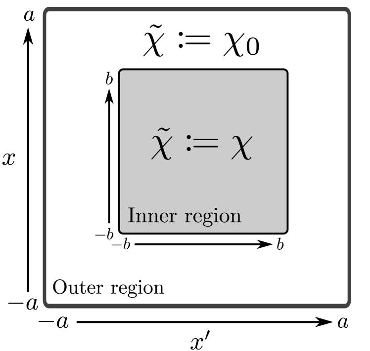
The xc kernel is now defined as the object that returns the truncated response function , rather than the interacting response function , upon solution of the Dyson equation. This leads to the following piecewise form for ,
The regularizing effect of the method presented above can be understood by examining the role of the truncation parameter . In particular, two extremes are considered, first, setting means the inversion of the response matrix at a given is performed over the whole domain, and hence is dominated by error due to excessive regions of nearly vanishing ground-state density; this error is hereafter referred to as the numerical error. Setting turns the truncated response function into the Kohn-Sham response function over the entire domain – an evidently unsatisfactory state of affairs – and error of this kind is referred to as method error. Whilst this need not be the case in principle, it is the case for the systems studied here that it is possible to choose such that an acceptable balance is struck between method error and numerical error. In other words, the truncated response function is able to retain all the physical properties of the interacting response function and ensure the computation of the resulting piecewise is well-conditioned. A discussion on the notion of error in the present context, including an elaboration of the method error and numerical error, is given in the supplemental material 444URL to be inserted.
One might take issue that the above piecewise expression for is spuriously discontinuous at the boundary of the inner and outer region, where the extent of this discontinuity depends on the long-range behavior of . However, we shall be concerned with the behavior of inside the inner region, i.e. the region where departure of the Hxc kernel from zero produces meaningful features in the output of the Dyson equation.
II.2.2 Eigenspace truncation
A second, related, method used in this work in order to regularize the computation of is to truncate the interacting response matrix in the eigenspace of the Kohn-Sham response matrix. This method is much more accurate than the real-space truncation, but is limited to Hermitian response matrices, i.e. response matrices constructed without an artificial broadening .
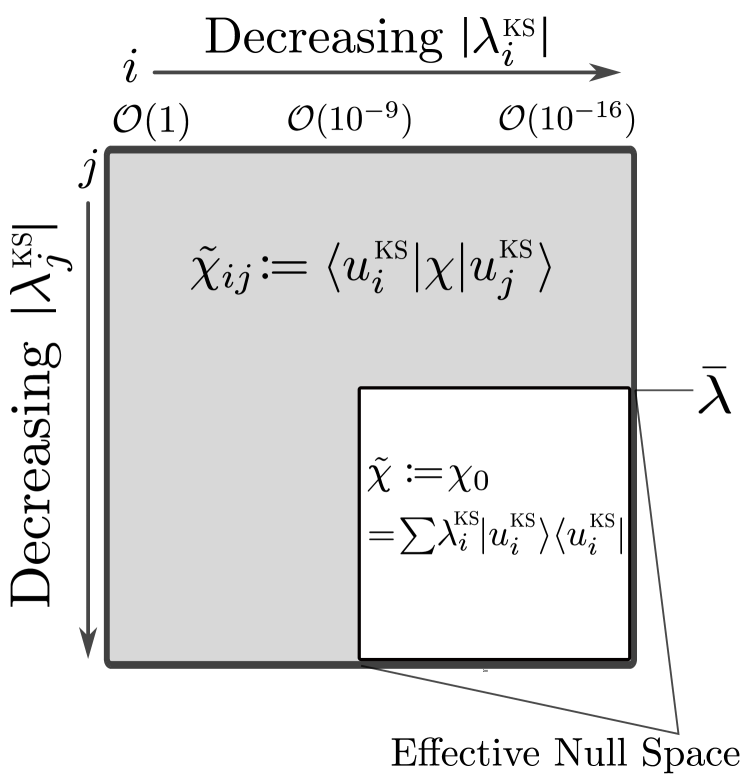
Consider the eigendecomposition of the interacting and Kohn-Sham response matrices at a given , where the eigenpairs are denoted and respectively. Consider further some value such that the effective null space, , is defined as the subspace spanned by eigenvectors whose eigenvalue has modulus below 555The formal definition of the effective null space is .. The assumption is now made that the truncated response matrix operates on vectors that are elements of the effective null space as the Kohn-Sham response matrix,
| (6) |
see Fig. 2. Given as the projection operator onto the effective null space, the expression in Eq. (6) is established as follows,
| (7) |
the first term on the right-hand side removes the effective null space from , and the second term ensures operates as intended on elements of the effective null space. Another view of this manipulation is that the truncated and Kohn-Sham response functions are required to share eigenvectors and eigenvalues inside the effective null space,
| (8) |
and the truncated response function is otherwise equal to the interacting response function, this is also depicted in Fig. 2.
The pseudoinverse [56] with cutoff , i.e. the eigendecomposition with eigenpairs below discarded, is now an exact procedure to obtain that recovers after solution of the Dyson equation,
| (9) |
where + denotes the pseudoinverse.
In direct analogy with the previous method, the parameter assumes the job of , namely, it parameterizes the extent of the truncation. The difference between the truncated response function Eq. (6) and the exact interacting response function is again given the name method error. Note that this approach is quite distinct from applying the pseudoinverse to the response functions in Eq. (5) – doing so would introduce much more error and the source of this error is not clear. On the contrary, the error inherent in the method presented here is identified as the extent to which the effective null space of the interacting and Kohn-Sham response functions do not overlap, and this error can be tracked without reference to using the method error.
Since the eigenspace truncation method is much more accurate than the real-space truncation method, results are given using the eigenspace truncation where possible. Although, visualization of the optical spectrum relies on evaluating the response functions slightly above the real axis in the frequency domain, along . This leads to response matrices that are complex-symmetric, and thus (weakly) non-Hermitian, in which case the real-space truncation method is used.
II.3 Gauge freedom
As noted in Refs. [28, 27, 57, 37], the following transformation
leaves the output of the Dyson equation unchanged, and thus we are, in principle, free to choose the arbitrary complex-valued functions and . All three transformations are a direct manifestation of the invariance of quantum Hamiltonian systems under a constant time-dependent shift of the potential. From the point of view of approximations, two xc kernels are equivalent if they exist within this family of functions 666Note that the quantities , where label indices of single-particle wavefunctions, are unique [27], and it is these quantities that form the input to the Casida equation [72], for example..
A preferred gauge is defined by Eq. (5), since the objects and are themselves invariant to a shift in the potential. The unique , modulo a constant shift (see below), defined in Eq. (5) can be considered the physical , and it is this definition of that is assumed in discussions on its various properties and limits [16, 15, 52, 53, 59]. To modify this using its gauge freedom changes its underlying structure; for example, setting gives spurious long-range behavior, and setting produces an that is not symmetric under interchange of . In this work, we illustrate as it is defined in Eq. (5), which also defines . The constant shift has special meaning, as it is itself an eigenvector of and with eigenvalue zero, i.e. the response functions are non-invertible in this direction. Since the Dyson equation is therefore silent regarding the value of , we anchor by requiring that, in the long-range limit, far outside the confined density, , and find that this limit is reliably achieved.
Having decided upon a preferred gauge, one can consider the possible consequences of this gauge freedom on matters of practical interest. An approximate that differs in relevant structure from the exact largely due to a change of gauge provides at least a partial explanation for the performance of a given approximate ; in Section III.4 we consider this line of inquiry.
III Results and discussion
III.1 Atom
Our first system consists of two interacting electrons confined in the atom-like potential, , within the domain a.u. An illustration of this system, and its associated numerical parameters, are given in the supplemental material. The purpose of the atom demonstration is two-fold. First, it constitutes a proof-of-concept, and defines a standard of accuracy to which the remainder of the calculations are held unless stated otherwise. Second, the optical spectrum of the atom is calculated in the range a.u., which includes many excitations beyond the first, and the efficacy of various approximations to are examined in relation to the optical spectrum.
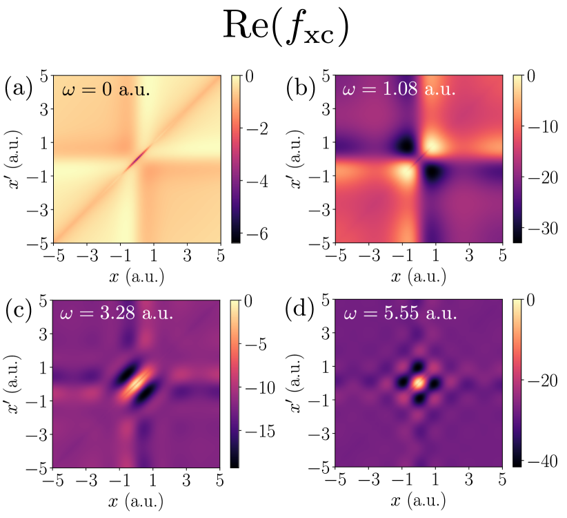
The exact , constructed using the real-space truncation method, is shown for the first three visible interacting excitations in the optical spectrum, and at a.u., in Fig. 3. The last is sometimes termed the exact adiabatic , and it correctly describes any system in which the response to a perturbation is essentially instantaneous, .
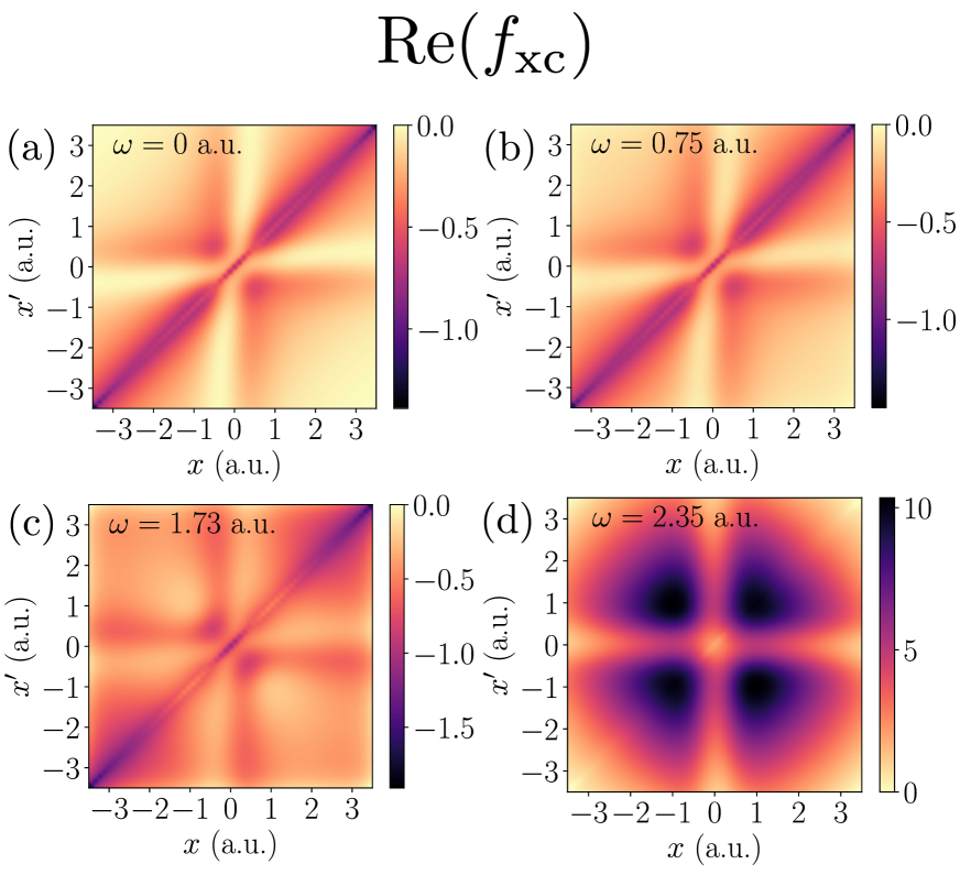
The real-space truncation parameter is chosen as a.u., meaning the inner region is defined as . It is important to stress that this choice of is not unique, and there exists some feasible range of within which itself is insensitive to changes. Moreover, within this feasible range, both the method error and numerical error are acceptable – a discussion on the precise quantification of error here is given in the supplemental material. The mean absolute error between the output of the Dyson equation, which is hereafter defined as
| (10) |
and the interacting response function is over the entire grid. The zero-force sum rule [2, 60] is used to further validate the numerics, which is discussed and illustrated in the supplemental material.
In order to extract the optical transition energies and transition rates, given a single-particle response function and xc kernel , one can construct the entire optical absorption spectrum Eq. (3) using the corresponding output of the Dyson equation, denoted , where is specified with some , see Fig. 4.
As established in [61, 62, 63], the exact Kohn-Sham single-particle transitions are in excellent agreement with the interacting transitions, but this agreement becomes increasingly poor at higher energies. An approach to understanding this is to consider the overlap between the final states involved in a given interacting and Kohn-Sham transition, where denotes the Slater determinant constructed from and Kohn-Sham single-particle states.
The overlap of the ground-state is , and the overlap of the final states involved in the first transition at a.u. is . The static correlation in the interacting state here is modest, meaning the interacting state has strong single-particle character, which leads to agreement between the low-energy transitions in the optical spectrum. At higher energies, the overlap decays by multiple orders of magnitude, however this is not the predominant source of error in higher energy transitions. Rather, interacting excitations that correspond to Kohn-Sham single-particle excitations out of the highest occupied state (the second) are much more accurate than single-particle excitations out of the first state. For example, the interacting excitation at a.u. in Fig. 4 is captured well with the Kohn-Sham excitation , whereas this is not true of the preceding interacting excitation. This is not surprising, as the highest occupied Kohn-Sham state has energy equal to minus the exact electron removal energy [64], and thus at least one energy involved in the transition is correct. This might often be the case, and to comment further would require additional many-body calculations.
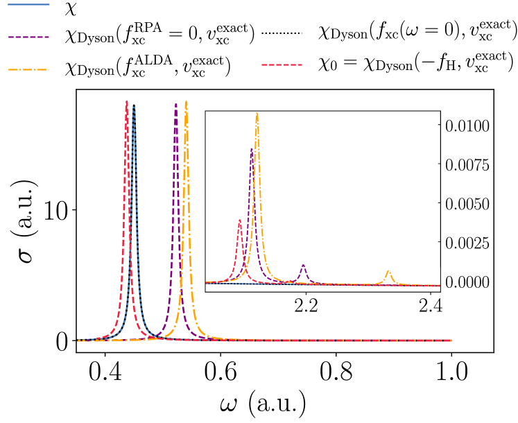
The following approximations are now considered: the RPA , an adiabatic LDA parameterized with reference to the homogeneous electron gas in [65], and the exact adiabatic xc kernel , Fig. 3(a). These approximations are used to solve the Dyson equation in conjunction with the exact Kohn-Sham response function. The atomic optical spectrum, using the aforementioned series of approximations, is shown in Fig. 5 for the first transition and a chosen higher energy transition.
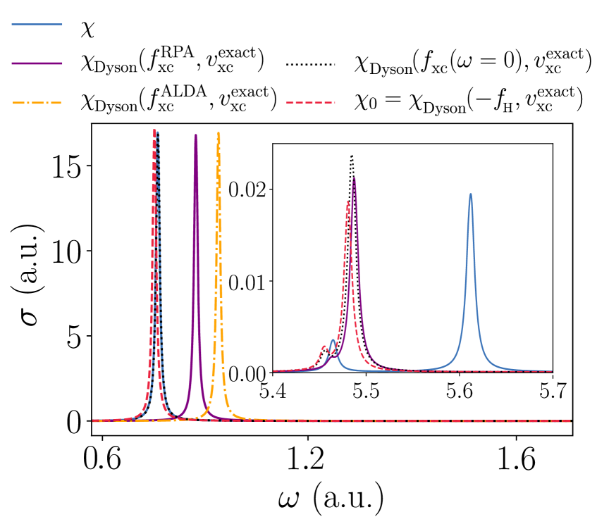
The exact adiabatic reproduces the first peak well, which reflects the fact that at the first excitation, Fig. 3(b), is visually indistinguishable from the exact adiabatic . This agreement demonstrates that, not only is the adiabatic approximation valid for low-energy transitions, but also the non-local spatial structure in the exact adiabatic is required in order to reproduce the low-energy peaks in the optical spectrum – in lacking this structure, both the RPA and adiabatic LDA significantly over-correct the underestimation of the non-interacting transition energy. At higher energies, i.e. beyond the third peak in the optical spectrum (not shown), all three approximations perform similarly, and do not improve matters significantly beyond the corresponding non-interacting peak. This behavior appears to be generic for all peaks observed up to a.u., namely, the transition energies output from the Dyson equation with these approximate xc kernels are bound to the quality of the non-interacting transition energies. Furthermore, the inset of Fig. 5 demonstrates that the exact adiabatic approximation gives an excitation energy that is worse than the other adiabatic approximations. This suggests that, in order to capture higher energy transitions, a frequency dependence is required, and in particular ‘improving’ the spatial structure of adiabatic approximations toward the exact adiabatic structure does not assist matters here.
As alluded to above, the exact adiabatic approximation ceases to out-perform the adiabatic LDA and RPA beyond the third transition in the optical spectrum, i.e. the same transition for which the corresponding exact departs from its adiabatic structure in a serious manner, Fig. 3. In fact, as the subsection to follow demonstrates, this violent departure from adiabaticity has a particular and fairly simple form, and its origin is understood in the context of eigenvalues of or that cross zero. The eigenvector corresponding to the eigenvalue that touches zero is a non--representable density perturbation at linear order.
III.2 Infinite potential well
The infinite potential well is defined with the external potential inside the domain a.u. (See supplemental material for the corresponding Kohn-Sham potential, density, and numerical parameters.) The numerical response functions for this system are well-conditioned and valid up to arbitrary , there are no regions of nearly vanishing density, and thus there is no significant numerical error present here.
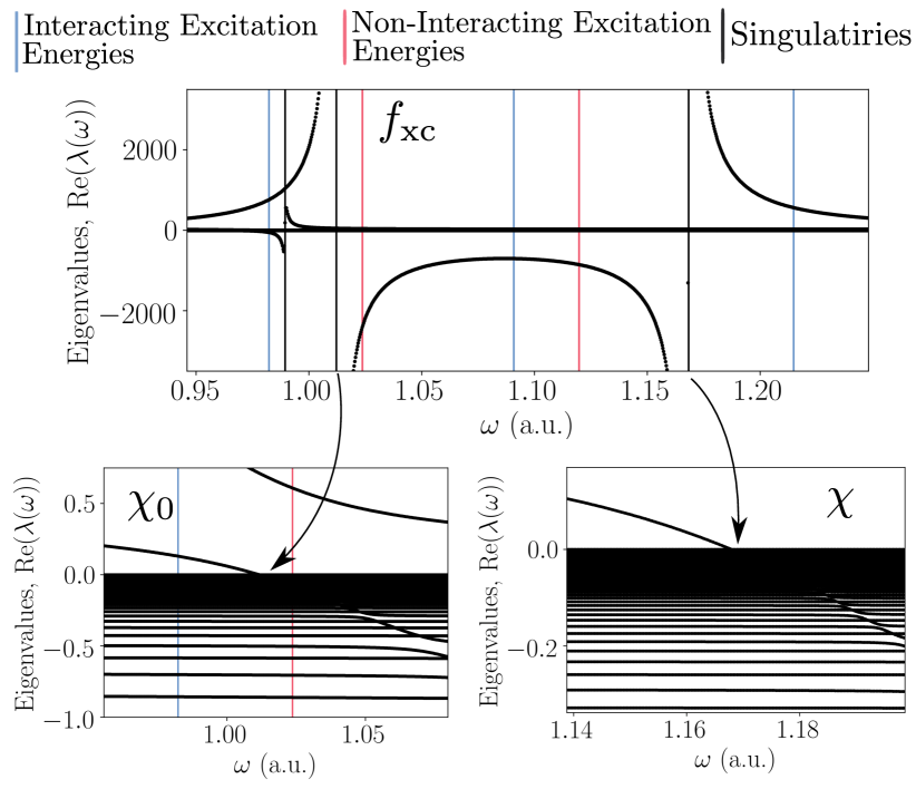
The non-adiabatic character of is illustrated up to a.u. in Fig. 6. As in the atom, exhibits little frequency dependence, until after the second transition. This behavior is related to the poles that occur in infinitesimally below the -axis [47, 27]. The eigenvalues of as a function of frequency are given in Fig. 7, and in particular, three divergences are shown (the singularities are tempered slightly by evaluating the response functions just above the real -axis). The lower panels of Fig. 7 demonstrate that these singularities coincide with a single eigenvalue of either the interacting or non-interacting response function crossing zero. Thus, the visual character of is dominated by the outer product of the eigenvector whose eigenvalue is either beginning to diverge, or recovering from a divergence. Moreover, nothing in principle is preventing these singularities in coming arbitrarily close to an interacting excitation – either can cross zero close to an interacting excitation, or itself can cross zero close to an interacting excitation 777The interacting response function diverges at an interacting excitation, but this does not, in a finite basis, prevent an eigenvalue from crossing zero at this energy under certain circumstances that are set out in the supplemental material.. Since most approximations lack these divergences, one can question the importance of these divergences in relation to optical properties.
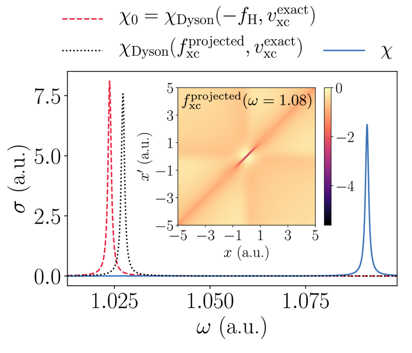
In order to determine the impact of the divergences in on the optical spectrum, we examine how the optical spectrum is affected after projecting out the divergent eigendirection in , but otherwise keeping identical (the details of this procedure are given in the supplemental material). This is tantamount to setting for some vector within the Hilbert space that is associated with the divergence.
The interacting excitation at a.u., see Fig. 7, is visible in the optical spectrum, and furthermore the character of at this energy, see Fig. 6, is dominated by the outer product of an eigenvector whose eigenvalue is much larger in magnitude than the rest, and between the two divergences at a.u. The removal of these divergences from across the energy range of interest, and subsequently solving the Dyson equation with the projected xc kernel , shifts the interacting optical peak back toward the non-interacting peak, Fig. 8. Conversely, the much weaker divergence at a.u., as seen in Fig. 7, has a tail that also yields an eigenvalue much larger in magnitude than the rest at the interacting excitation, and removal of this divergence produces no change in the optical spectrum, i.e. this eigenvector is not relevant for capturing the transition in question. In the inset of Fig. 8, the visual character of is shown at the interacting excitation a.u. after the divergences visible in Fig. 7 have been removed. Underneath these divergences, is indistinguishable from the adiabatic , meaning the frequency dependence of in this system is largely due to its pole structure. These results suggest that functional approximations that do not capture the non-adiabatic pole structure of will struggle to improve matters beyond the non-interacting peaks for certain transitions.
A further point of note is that there are many more zeros in the interacting response function than the non-interacting response function, as a simple counting argument is sufficient to demonstrate. All eigenvalues of the response functions begin negative [47], and each excitation brings a negative eigenvalue to a positive eigenvalue across a divergence, which otherwise evolves as a continuous function of . For two electrons discretized with a basis set of dimension , there are interacting excitations, and non-interacting excitations, the difference being made up of double (triple, etc. with more than two electrons) excitations that are notoriously not present in the Kohn-Sham response function [21]. Therefore, there are a great deal more eigenvalues that must pass through zero in the interacting response function, and moreover, these eigenvalues that cross zero are connected to the excitations that require them to do so – an account of the precise conditions under which this occurs is given in the supplemental material using a two-state model, see also [65].
In Fig. 7, there are three divergences, two of which are paired at a.u., meaning the zero in the non-interacting response function is a shifted version of the zero in the interacting response function; such behavior can be related to single excitations. There also exists an unpaired divergence at a.u. related to the excitation at a.u. which has double excitation character. That is, the overlap between the final state involved in this transition and the Slater determinant is .
It is perhaps, then, no surprise that removal of the eigenvector and eigenvalue whose source is the unpaired divergence did not alter the visible (single excitation) transition in Fig. 8. In fact, the pole in the interacting response function relating to the double excitation disappears with removal of the unpaired divergence, and so this divergence, and its surrounding character, is important in order to capture the transition for which it is relevant. The xc kernel exhibits unpaired divergences after all double excitations up to a.u. at frequencies slightly higher than the interacting double excitation energy. Refs. [21, 23] derive, under certain assumptions, the necessarily divergent character of around a double excitation. The above analysis reveals that divergences in are, in fact, common and associated with the neighborhood containing multiple and single excitations alike.
III.3 Quantum harmonic oscillator
The quantum harmonic oscillator is defined in the domain a.u. with the potential where a.u. (See supplemental material for the corresponding exact Kohn-Sham potential, the interacting ground-state density, and the numerical parameters.)
First, the spatial structure, and in particular the long-range behavior [16], of the exact is examined. The delicate nature of the numerics involved in computing the exact is brought to the fore when attempting to capture its long-range limit. The ill-conditioning in the response matrices can be identified with regions of nearly vanishing ground-state density, see Section II.2, and it is precisely in these regions that we expect to observe the long-range character of . However, , when evaluated outside some central region where we can be confident there is little-to-no numerical error, diverges in a manner that is not consistent with the known long-range limit of . This spurious divergence in does not much affect the accuracy of the output of the Dyson equation, , because the Dyson equation Eq. (10) involves the matrix product , and the divergent regions of operate on the nearly vanishing regions of .
If we are to observe the long-range limit of in the present context, the region where the numerical error is low must overlap with the region where the long-range limit is observed. This is the case for the exact adiabatic , which is shown, together with slices of along a particular axis, in Fig. 9 and Fig. 10.
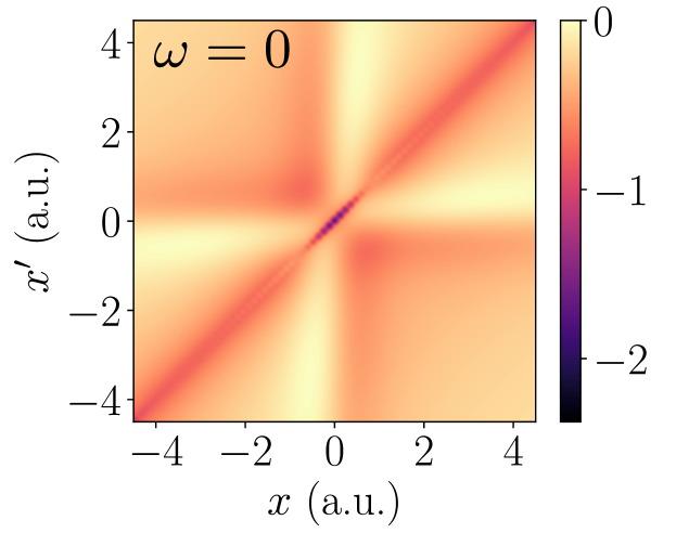
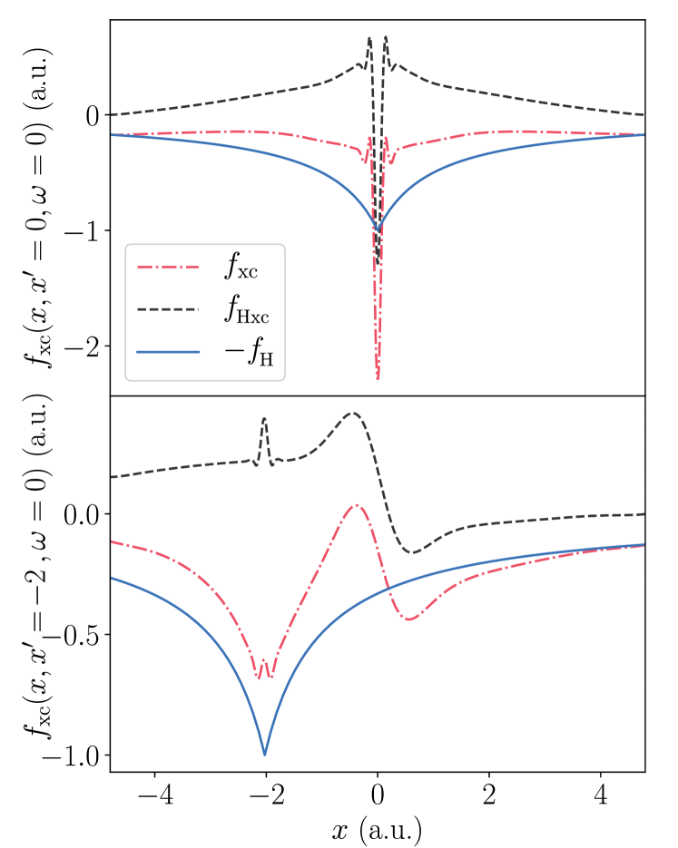
The center-most region of the domain is where exchange and correlation effects are most important, and in this region exhibits a strong local response that quickly decays as . Since this region can be interpreted as the most crucial for recovering accurate observable properties from the Dyson equation, this observation supports, at least in part, local approximations to , such as the adiabatic LDA.
The non-local structure of at a.u. can be seen most clearly in the lower panel of Fig. 10, where perturbations in the density outside the center-most region cause a significant change in the exchange-correlation potential inside the center-most region. The failure of the adiabatic LDA to capture this non-local response leads to fairly poor agreement between the exact and approximate transition energies, which is seen for the atom in Fig. 5, and illustrated for the quantum harmonic oscillator below 888It is possible that the particular form of the non-local functionals considered in [73, 13], in which , can capture certain features of the adiabatic non-local response depicted in Fig. 9 and Fig. 10..
The long-range limit is explored in Fig. 10 along both a.u. and a.u. Due to the rapid decay of the ground-state density in the quantum harmonic oscillator, convergence of toward along a.u. is not directly observed in the limit – the atom, whose ground-state density does not decay as quickly, converges toward in both the positive and negative limits (see supplemental material). It is known that the long-range limit of , in both finite and periodic systems, satisfies [16, 15, 52, 53], where is a frequency-dependent constant that reflects dielectric screening in the system. Therefore, one expects in finite systems, and at lower frequencies, where the numerical methodology provides a robust long-range limit, our observations are consistent with this, see Fig. 10.
To conclude matters for the quantum harmonic oscillator, we examine its optical absorption spectrum, and in particular highlight a failing of the approximations considered in this work when compared to the exact and exact adiabatic xc kernels. The optical absorption spectrum, using the same range of approximations discussed in the case of the atom, is shown in Fig. 11. In the non-interacting quantum harmonic oscillator, all transitions but the first are disallowed, otherwise known as its selection rules. The inclusion of the Coulomb interaction lifts these special symmetries of the non-interacting quantum harmonic oscillator, but not enough for the previously disallowed transitions to be observed in the optical spectrum – the dipole matrix elements for these allowed transitions are . On the other hand, the exact Kohn-Sham potential differs significantly from the harmonic form, which creates a series of visible peaks beyond the first in the optical spectrum; the transition rates for these transitions are vastly overestimated.
In this situation, the RPA and adiabatic LDA do not achieve the required strong suppression of the optical peaks. Interestingly, the exact adiabatic kernel, as seen in Fig. 9, is able to reproduce the exact optical spectrum across the entire frequency range considered a.u., presumably due to the correct oscillator strengths used in its construction. This suggests that, in cases where the exact system possesses heavily suppressed transitions, perhaps due to symmetries that are not shared by the Kohn-Sham system, the typical approximations are insufficient to recover the exact state of affairs, but improvement of their non-local spatial structure toward the exact adiabatic kernel can assist matters.
III.4 Gauge freedom
Two xc kernels that differ in structure that is predominantly captured with the gauge transform defined in Section II.3 provides an explanation for the approximate agreement between the derived properties of the two xc kernels in question. This possibility is now considered, and in fact we shall demonstrate that the gauge freedom of is not sufficient to explain the similarity observed between, for example, the optical properties calculated using the adiabatic LDA and RPA in Section III. Moreover, the particular form of the non-local spatial structure within the exact is in general not possible to capture with this gauge freedom, and it is unlikely that this line of reasoning is able to explain the efficacy of approximations of any kind.
In order to demonstrate this, an optimal gauge is defined that transforms, in as much as is possible, one xc kernel into another using the gauge freedom, i.e. it brings one toward another in a particular matrix norm. The definition and derivation of the optimal gauge is given in the relevant section of the supplemental material. Furthermore, an illustration of the optimal gauge transform for each of the examples to follow is also provided in the supplemental material. The atom of Section III is considered, and in particular the optimal gauge is found in order to match the RPA, , with the adiabatic LDA used in this work, [65]. As discussed in Section II.3, the vectors and introduce an unavoidable degree of non-locality, and the local spatial structure of the adiabatic LDA simply cannot be reproduced with a gauge transform of this kind applied to the RPA.
The story remains much the same when an attempt is made to match the adiabatic LDA xc kernel to the exact adiabatic xc kernel for the atom, . The particular form of the spatial non-locality in the exact adiabatic xc kernel does not lend itself to the fairly inflexible structural freedom afforded by the functions and . This conclusion holds true for almost all the xc kernels examined in this work, namely, the spatial profile of the exact at any is not possible to reproduce with a gauge transform applied to the adiabatic LDA or RPA, despite, at high frequencies, the similarity of the derived optical spectra from these approximations.
A final remark is given in relation to the divergences in studied in the previous section. The xc kernel around a divergence is approximately of the form of an outer product , where is the eigenvector of that is diverging. The xc kernel is therefore mostly composed of degrees of freedom, a state of affairs that is a priori much more amenable to the gauge freedom. In fact, the first pole in the of the atom, i.e. the beginning of the non-adiabatic behavior, see panel (d) of Fig. 3, is non-divergent after the optimal gauge is applied. This divergence therefore does not affect observable properties such as its associated optical peak, and indeed the exact adiabatic kernel is able to capture this peak, despite it existing squarely within the divergence. However, such a situation is not detected again for the remainder of the divergences.
III.5 Exchange-correlation potential versus exchange-correlation kernel
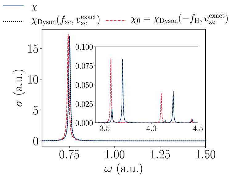
In finite systems, it is the conventional wisdom that an accurate ground-state xc potential is more important for capturing the interacting excitation spectrum than a sophisticated [16, 15, 68, 69, 70]. The effect of an improved treatment of exchange and correlation in the ground state is shown in Fig. 12, which demonstrates the optical spectrum for the atomic system calculated from the non-interacting response function at various levels of approximation. The transition energies and rates calculated from the exact Kohn-Sham system are considerably closer to the exact transitions than, for example, Hartree theory, which is increasingly poor at higher energies.
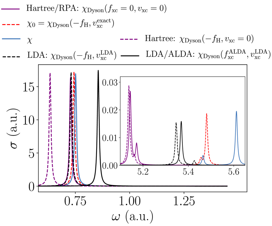
These non-interacting response functions can be used, in conjunction with their corresponding , to solve the Dyson equation, thus shifting the position and weight of the peaks. An xc kernel functional corresponds to an xc potential functional if it is the second functional derivative of the xc potential with respect to the density. Thus, the RPA xc kernel corresponds to Hartree theory, and the adiabatic LDA xc kernel corresponds to the ground-state LDA from which it came. To use an xc kernel that does not correspond to the ground-state xc potential can violate various exact conditions [71] – this is evidently the case here for the zero-force sum rule.
The aforementioned conventional wisdom is exhibited clearly in Fig. 12, namely, use of a corresponding is only able to improve matters slightly beyond the non-interacting peaks, which is most visible at higher frequencies. For this reason, even when using an incompatible , the calculation benefits from an improved treatment of ground-state exchange and correlation. This is evidenced in the case of the atom in Section III, where using the RPA and adiabatic LDA xc kernels in conjunction with the exact Kohn-Sham ground-state yields a more accurate optical spectrum than if one were to attempt to keep the xc potential and xc kernel compatible.
IV Conclusions
We have calculated and analyzed the spatial and frequency dependence of the exact xc kernel of time-dependent DFT for three one-dimensional model systems: an atom, an infinite potential well, and a quantum harmonic oscillator. A set of numerical methods is designed to ensure numerical robustness.
The xc kernel exhibits a significant non-local spatial structure at all frequencies, including at , i.e. the exact adiabatic . In lacking this structure, local approximations to are found to be insufficient for recovering the lowest energy excitations, whereas the exact adiabatic xc kernel performs well. However, beyond the lowest few excitations, all the approximations considered here – the exact adiabatic xc kernel, the RPA, and the adiabatic LDA – are equally poor, and do not generally improve the optical spectrum obtained directly from the non-interacting Kohn-Sham response function (that is, setting to zero everywhere). A notable exception is the quantum harmonic oscillator, whose optical transitions beyond the first are heavily suppressed, a feature that the exact adiabatic xc kernel is able to capture. In general, improvement of the spatial structure of adiabatic xc kernel approximations toward the exact adiabatic xc kernel is expected to assist matters for the lowest energy transitions, but beyond these transitions the lack of frequency dependence hinders all adiabatic xc kernels. In addition, the long-range limit of for finite systems is confirmed, although the long-range character of is demonstrated to be unimportant in the present context, in contrast to its character within and around the region of high density.
Drastic non-adiabatic behavior is observed in for all systems studied in this work, and is, to a considerable extent, attributable to specific aspects of its analytic structure as a function of . (Simple) poles in , related to certain interacting or non-interacting transitions that necessitate them, can in practice appear close to interacting excitations, for example, between two nearly degenerate charge-transfer excitations in a double-well system [50]. It is possible that a gauge transform can remove the divergence in specific cases without affecting the optical spectrum, but this is the exception rather than the rule. If is kept identical apart from removal of the diverging eigenvalue and its associated eigenvector, then can be rendered unable to capture the relevant transition. This suggests that an approximation that does not attempt to exhibit the non-adiabatic pole structure of the exact cannot reproduce transitions with energies higher than the first few excitations. This is the case for single, double, triple, and so on, excitations alike. The fact that these divergences can be related to certain excitations that necessitate them provides a new perspective on the divergent character of that is known to exist around double excitations [21, 36].
In general, the subtle spatial structure of the exact cannot be captured by applying a gauge transformation to one of the usual kernel approximations. However, the divergent -dependence discussed in the previous paragraph is more amenable to the gauge freedom. Indeed, in the case of the atom, the first divergence (around the third peak in the optical spectrum) turns out to be related to the exact adiabatic with a gauge transform. Hence, the exact adiabatic approximation is able to describe the third peak in the optical spectrum, despite the significant frequency dependence of around this peak.
As noted earlier in this section, the simple non-interacting kernel often yields surprisingly good spectra, provided that the exact Kohn-Sham potential, or a good approximation to it, is used to calculate . This is in part due to the fact that the exact Kohn-Sham transitions are, in certain circumstances, good approximations to the interacting transitions [70]. By extension, in practical calculations, effort may be usefully devoted to improving approximations used for and individually, without an overriding need to maintain one as the functional derivative of the other. The quality of is of particular importance, as previous authors have observed in specific cases [16, 15, 68, 69, 70].
In systems where predictive spectral accuracy beyond that provided by the simplest kernels is required, note should be taken of the intricate spatial non-locality and analytic structure as a function of exhibited by the exact kernels calculated in this paper. Approximate kernels that are spatially local (whether local-density or not), and/or exhibit no more than a gentle variation with , are unlikely to prove adequate for calculating optical spectra and other aspects of the density response function. A fruitful direction appears to be kernels that are obtained by making a connection between the time-dependent DFT description and some level of many-body perturbation theory, such as the kernel obtained from the Bethe-Salpeter equation presented in [26], since non-locality and frequency dependence emerge automatically from even the simplest level of many-body perturbation theory.
Acknowledgements.
The authors thank Michael Hutcheon and Matt Smith for helpful discussions. N.D.W is supported by the EPSRC Centre for Doctoral Training in Computational Methods for Materials Science for funding under grant number EP/L015552/1.References
- Martin et al. [2016] R. M. Martin, L. Reining, and D. M. Ceperley, Interacting Electrons Theory and Computational Approaches (Cambridge University Press, 2016).
- Ullrich [2012] C. A. Ullrich, Time-dependent density-functional theory : concepts and applications (Oxford University Press, 2012) p. 526.
- Marques et al. [2006] M. A. Marques, C. A. Ullrich, F. Nogueira, A. Rubio, K. Burke, and E. K. U. Gross, eds., Time-Dependent Density Functional Theory, Lecture Notes in Physics, Vol. 706 (Springer Berlin Heidelberg, Berlin, Heidelberg, 2006).
- Ullrich and Hui Yang [2014] C. A. Ullrich and Z. Hui Yang, Brazilian Journal of Physics 44, 154 (2014).
- Burke et al. [2005] K. Burke, J. Werschnik, and E. K. Gross, Journal of Chemical Physics 123, 062206 (2005).
- Casida and Huix-Rotllant [2012] M. Casida and M. Huix-Rotllant, Annual Review of Physical Chemistry 63, 287 (2012).
- Marques and Gross [2004] M. Marques and E. Gross, Annual Review of Physical Chemistry 55, 427 (2004).
- Gross and Kohn [1990] E. Gross and W. Kohn, in Density Functional Theory of Many-Fermion Systems, Advances in Quantum Chemistry, Vol. 21, edited by P.-O. Löwdin (Academic Press, 1990) pp. 255 – 291.
- Runge and Gross [1984] E. Runge and E. K. Gross, Physical Review Letters 52, 997 (1984).
- van Leeuwen [1999] R. van Leeuwen, Physical Review Letters 82, 3863 (1999).
- Onida et al. [2002] G. Onida, L. Reining, and A. Rubio, Reviews of Modern Physics 74, 601 (2002).
- Görling [2019] A. Görling, Physical Review B 99, 235120 (2019).
- Olsen et al. [2019] T. Olsen, C. E. Patrick, J. E. Bates, A. Ruzsinszky, and K. S. Thygesen, npj Computational Materials 5, 2057 (2019).
- Note [1] Hartree atomic units are used throughout.
- Botti et al. [2007] S. Botti, A. Schindlmayr, R. Del Sole, and L. Reining, Reports on Progress in Physics 70, 357 (2007).
- Ullrich and Yang [2016] C. A. Ullrich and Z. H. Yang, Topics in Current Chemistry 368, 185 (2016).
- Gavrilenko and Bechstedt [1997] V. I. Gavrilenko and F. Bechstedt, Phys. Rev. B 55, 4343 (1997).
- Corradini et al. [1998] M. Corradini, R. Del Sole, G. Onida, and M. Palummo, Phys. Rev. B 57, 14569 (1998).
- Moroni et al. [1995] S. Moroni, D. M. Ceperley, and G. Senatore, Phys. Rev. Lett. 75, 689 (1995).
- Maitra et al. [2002] N. T. Maitra, K. Burke, and C. Woodward, Phys. Rev. Lett. 89, 023002 (2002).
- Maitra et al. [2004] N. T. Maitra, F. Zhang, R. J. Cave, and K. Burke, The Journal of Chemical Physics 120, 5932 (2004).
- Elliott et al. [2011] P. Elliott, S. Goldson, C. Canahui, and N. T. Maitra, Chemical Physics 391, 110 (2011), arXiv:1101.3379 .
- Cave et al. [2004] R. J. Cave, F. Zhang, N. T. Maitra, and K. Burke, Chemical Physics Letters 389, 39 (2004).
- Reining et al. [2002] L. Reining, V. Olevano, A. Rubio, A. Rubio, and G. Onida, Physical Review Letters 88, 4 (2002).
- Marini et al. [2003] A. Marini, R. Del Sole, and A. Rubio, Physical Review Letters 91, 256402 (2003), arXiv:0310495 [cond-mat] .
- Romaniello et al. [2009] P. Romaniello, D. Sangalli, J. A. Berger, F. Sottile, L. G. Molinari, L. Reining, and G. Onida, Journal of Chemical Physics 130, 044108 (2009).
- Hellgren and Von Barth [2009] M. Hellgren and U. Von Barth, Journal of Chemical Physics 131, 044110 (2009).
- Hellgren and von Barth [2008] M. Hellgren and U. von Barth, Phys. Rev. B 78, 115107 (2008).
- Kim and Görling [2002] Y.-H. Kim and A. Görling, Phys. Rev. Lett. 89, 096402 (2002).
- Görling [1999] A. Görling, Phys. Rev. Lett. 83, 5459 (1999).
- Görling [1998] A. Görling, Physical Review A - Atomic, Molecular, and Optical Physics 57, 3433 (1998).
- Del Sole et al. [2003] R. Del Sole, G. Adragna, V. Olevano, and L. Reining, Physical Review B - Condensed Matter and Materials Physics 67, 045207 (2003).
- Botti et al. [2004] S. Botti, F. Sottile, N. Vast, V. Olevano, L. Reining, H.-C. Weissker, A. Rubio, G. Onida, R. Del Sole, and R. W. Godby, Phys. Rev. B 69, 155112 (2004).
- Ruggenthaler et al. [2013] M. Ruggenthaler, S. E. Nielsen, and R. Van Leeuwen, Physical Review A - Atomic, Molecular, and Optical Physics 88, 022512 (2013).
- Maitra and Tempel [2006] N. T. Maitra and D. G. Tempel, Journal of Chemical Physics 125, 184111 (2006).
- Gritsenko and Jan Baerends [2009] O. V. Gritsenko and E. Jan Baerends, Physical Chemistry Chemical Physics 11, 4640 (2009).
- Aryasetiawan and Gunnarsson [2002] F. Aryasetiawan and O. Gunnarsson, Phys. Rev. B 66, 165119 (2002).
- Carrascal et al. [2018] D. J. Carrascal, J. Ferrer, N. Maitra, and K. Burke, European Physical Journal B 91, 142 (2018).
- Turkowski and Rahman [2014] V. Turkowski and T. S. Rahman, Journal of Physics Condensed Matter 26, 6 (2014).
- Fuks and Maitra [2014] J. I. Fuks and N. T. Maitra, Phys. Chem. Chem. Phys. 16, 14504 (2014).
- Thiele and Kümmel [2009] M. Thiele and S. Kümmel, Physical Review A - Atomic, Molecular, and Optical Physics 80, 012514 (2009).
- Thiele and Kümmel [2014] M. Thiele and S. Kümmel, Physical Review Letters 112, 083001 (2014).
- Entwistle and Godby [2019] M. T. Entwistle and R. W. Godby, Physical Review B 99, 161102 (2019).
- Hodgson et al. [2013] M. J. Hodgson, J. D. Ramsden, J. B. Chapman, P. Lillystone, and R. W. Godby, Physical Review B - Condensed Matter and Materials Physics 88, 241102 (2013).
- Ruggenthaler et al. [2015] M. Ruggenthaler, M. Penz, and R. van Leeuwen, Journal of Physics: Condensed Matter 27, 203202 (2015).
- Tarantola [2005] A. Tarantola, Inverse Problem Theory and Methods for Model Parameter Estimation (Society for Industrial and Applied Mathematics, 2005).
- Van Leeuwen [2001] R. Van Leeuwen, International Journal of Modern Physics B 15, 1969 (2001).
- Mearns and Kohn [1987] D. Mearns and W. Kohn, Physical Review A 35, 4796 (1987).
- Note [2] For example, the constant perturbation oscillating with frequency produces no response in the density at all orders, including at first order.
- Note [3] We observed this situation in a double-well system that we explored as background to the present study.
- Maitra [2017] N. T. Maitra, Journal of Physics Condensed Matter 29, 423001 (2017).
- Ghosez et al. [1997] P. Ghosez, X. Gonze, and R. Godby, Physical Review B - Condensed Matter and Materials Physics 56, 12811 (1997).
- Byun et al. [2020] Y.-M. Byun, J. Sun, and C. A. Ullrich, Electronic Structure 2, 023002 (2020).
- Note [4] URL to be inserted.
- Note [5] The formal definition of the effective null space is .
- Ben-Isreal A. [2003] G. T. N. E. Ben-Isreal A., Generalized Inverses (Springer-Verlag, 2003).
- Hellgren and Gross [2012] M. Hellgren and E. K. Gross, Physical Review A - Atomic, Molecular, and Optical Physics 85, 022514 (2012).
- Note [6] Note that the quantities , where label indices of single-particle wavefunctions, are unique [27], and it is these quantities that form the input to the Casida equation [72], for example.
- Godby and Needs [1989] R. W. Godby and R. J. Needs, Physical Review Letters 62, 1169 (1989).
- Wagner et al. [2012] L. O. Wagner, Z.-h. Yang, and K. Burke, in Fundamentals of Time-Dependent Density Functional Theory (Springer-Verlag Berlin Heidelberg, 2012) pp. 101–123.
- Appel et al. [2003] H. Appel, E. K. Gross, and K. Burke, Physical Review Letters 90, 4 (2003).
- Savin et al. [1998] A. Savin, C. J. Umrigar, and X. Gonze, Chemical Physics Letters 288, 391 (1998).
- Al-Sharif et al. [1998] A. I. Al-Sharif, R. Resta, and C. J. Umrigar, Physical Review A - Atomic, Molecular, and Optical Physics 57, 2466 (1998).
- Perdew et al. [1982] J. P. Perdew, R. G. Parr, M. Levy, and J. L. Balduz, Phys. Rev. Lett. 49, 1691 (1982).
- Entwistle et al. [2018] M. T. Entwistle, M. Casula, and R. W. Godby, Phys. Rev. B 97, 235143 (2018).
- Note [7] The interacting response function diverges at an interacting excitation, but this does not, in a finite basis, prevent an eigenvalue from crossing zero at this energy under certain circumstances that are set out in the supplemental material.
- Note [8] It is possible that the particular form of the non-local functionals considered in [73, 13], in which , can capture certain features of the adiabatic non-local response depicted in Fig. 9 and Fig. 10.
- Marques and Gross [2003] M. A. L. Marques and E. K. U. Gross, in A Primer in Density Functional Theory (Springer, Berlin, Heidelberg, 2003) pp. 144–184.
- Marques et al. [2001] M. A. Marques, A. Castro, and A. Rubio, Journal of Chemical Physics 115, 3006 (2001).
- Petersilka et al. [2000] M. Petersilka, E. K. U. Gross, and K. Burke, International Journal of Quantum Chemistry 80, 534 (2000).
- Liebsch [1985] A. Liebsch, Physical Review B 32, 6255 (1985).
- Casida [1995] M. E. Casida, Recent Advances in Density Functional Methods (World Scientific Publishing, 1995) pp. 155–192.
- Olsen and Thygesen [2014] T. Olsen and K. S. Thygesen, Physical Review Letters 112, 203001 (2014).