Insights into photosynthetic energy transfer gained from free-energy structure: Coherent transport, incoherent hopping, and vibrational assistance revisited

To describe EET, we restrict the electronic spectra of the $m$-th pigment in a PPC to the ground state, $\lvert\varphi_{m{\mathrm{g}}}\rangle$, and the first excited state, $\lvert\varphi_{m\mathrm{e}}\rangle$, although higher excited states may result in nonlinear spectroscopic signals. Thus, the Hamiltonian of a PPC comprising $N$ pigments is expressed as $\hat{H}_{\rm PPC}=\sum_{m=1}^{N}\sum_{a=\mathrm{g},\mathrm{e}}\hat{H}_{ma}(x_{m})\lvert\varphi_{ma}\rangle\langle\varphi_{ma}\rvert+\sum_{m=1}^{N}\sum_{n=1}^{N}J_{mn}\lvert\varphi_{m\mathrm{e}}\rangle\langle\varphi_{m\mathrm{g}}\rvert\otimes\lvert\varphi_{n\mathrm{g}}\rangle\langle\varphi_{n\mathrm{e}}\rvert$. Here, $\hat{H}_{ma}(x_{m})$ represents the diabatic Hamiltonian for the environmental and intramolecular vibrational degrees of freedom (DoFs), $x_{m}$, when the system is in the $\lvert\varphi_{ma}\rangle$ state for $a=\mathrm{g}$ and $a=\mathrm{e}$. The electronic coupling between the pigments, $J_{mn}$, may also be modulated by the environmental and nuclear DoFs. In the following, however, it is assumed that the nuclear dependence of $J_{mn}$ is vanishingly small and the Condon-like approximation is employed as usual. The Franck–Condon transition energy of the $m$-th pigment is obtained as

where the canonical average has been introduced, $\langle\dots\rangle_{ma}=\mathrm{tr}(\dots\rho_{ma}^{\rm eq})$ with the environmental equilibrium state for the $\lvert\varphi_{ma}\rangle$ state, $\hat{\rho}_{ma}^{\rm eq}=\mathrm{e}^{-\beta\hat{H}_{ma}}/\mathrm{tr}\,\mathrm{e}^{-\beta\hat{H}_{ma}}$. Here, $\beta$ is the inverse temperature, $1/k_{\rm B}T$. The electronic energy of each diabatic state experiences fluctuations caused by the environmental and nuclear dynamics; these dynamics are described by the collective energy gap coordinate, such that

By definition, the mean values of the coordinate with respect to the electronic ground and excited states are given by

respectively, where the emission energy has been introduced,

For the sake of simplicity, the contribution of intramolecular vibrational modes are not considered at the current stage. The vibrational contribution will be discussed in Sec. III.3.

Let the probability distribution function for the classical collective energy gap coordinate $X_{m}$ be $P_{ma}(X_{m})$ when the system is in the $\lvert\varphi_{ma}\rangle$ state. The corresponding free energy is given by $F_{ma}(X_{m})=-k_{\rm B}T\ln P_{ma}(X_{m})+\mathrm{const}$. In this work, it is assumed that the environmentally induced fluctuations can be described as a Gaussian process.Kubo et al. (1985) Under the assumption that $X_{m}$ is described as a Gaussian random variable, the probability distribution function $P_{ma}(X_{m})$ is expressed as a Gaussian function,

where $\sigma_{ma}^{2}$ denotes the variance of $X_{m}$ with respect to the equilibrium state associated with the $\lvert\varphi_{ma}\rangle$ state. Hence, the free energy with respect to $X_{m}$ is given as a quadratic function,

and the environmental reorganization energy associated with the optical transition to the $\lvert\varphi_{ma}\rangle$ state, $E_{ma}^{\rm R}=\lvert F_{ma}(\mu_{m{\mathrm{g}}})-F_{ma}(\mu_{m{\mathrm{e}}})\rvert$, is obtained as

As described in Appendix A, the relation $\mu_{m\mathrm{e}}=-\beta\sigma_{m\mathrm{g}}^{2}$ is valid under the Gaussian assumption, and the variances and hence the reorganization energies are independent of the electronic states, namely $\sigma_{m{\mathrm{g}}}^{2}=\sigma_{m{\mathrm{e}}}^{2}=\sigma_{m}^{2}$ and $E_{m{\mathrm{g}}}^{\rm R}=E_{m{\mathrm{e}}}^{\rm R}=E_{m}^{\rm R}$. Hence, eqs (2.3) and (2.7) lead to

and a simple relation among the variance of the fluctuations $\sigma_{m}^{2}$, temperature $T$, and the reorganization energy $E^{\rm R}$ is obtained:

Consequently, the expressions of the free energies for the electronic ground and excited states are obtained as Marchi et al. (1993); Chandler (1998)

These expressions are consistent with the environmental dynamics in which the electronic and environmental states relax from the equilibrium configuration with respect to the $\lvert\varphi_{m{\mathrm{g}}}\rangle$ state and to the actual equilibrium configuration in the $\lvert\varphi_{m{\mathrm{e}}}\rangle$ state after the vertical Franck–Condon excitation, as is formulated in Appendix B.

There is no experimental evidence of nonadiabatic transitions and radiative/nonradiative decays between $\lvert\varphi_{m{\mathrm{e}}}\rangle$ and $\lvert\varphi_{m{\mathrm{g}}}\rangle$ in light-harvesting pigment-protein complexes on the picosecond timescales, and hence, we organize the product states in order of elementary excitation number. The overall ground state with zero excitation is $\lvert 0\rangle=\prod_{m=1}^{N}\lvert\varphi_{m{\mathrm{g}}}\rangle$, whereas the presence of a single excitation at the $m$-th pigment is expressed as $\lvert m\rangle=\lvert\varphi_{m{\mathrm{e}}}\rangle\prod_{k(\neq m)}\lvert\varphi_{kg}\rangle$. The corresponding expansion of the complete PPC Hamiltonian yields $\hat{H}_{\rm PPC}=\hat{H}_{\rm PPC}^{(0)}+\hat{H}_{\rm PPC}^{(1)}+\dots$, where $\hat{H}_{\rm PPC}^{(n)}$ describes $n$-excitation manifold comprising $n$ elementary excitations. The Hamiltonian of the zero-excitation manifold is

with $\hat{H}^{(0)}=\sum_{m=1}^{N}\hat{H}_{m{\mathrm{g}}}$. The Hamiltonian of the one-excitation manifold takes the form,

where $\hat{H}_{m}$ has been introduced as

The intensity of sunlight is weak and, thus, the single-excitation manifold is of primary importance under physiological conditions, although nonlinear spectroscopic techniques such as 2D electronic spectroscopy can populate higher excitation manifolds.

Correspondingly to the Hamiltonians, the free energy surfaces for the zero- and one-excitation manifolds are given as

where the free-energy $F_{m}({\bf X})$ has been introduced correspondingly to the Hamiltonian in eq (3.3) as

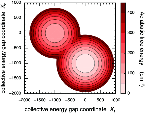
For simplicity, the study addresses a dimer comprising pigments 1 and 2 and considers the two-dimensional reaction coordinate space, ${\bf X}=(X_{1},X_{2})$. In this case, eq (3.5) is easily diagonalized, and the adiabatic free energy surfaces in the one-excitation manifold are obtained. Figure 1 draws the adiabatic free energy surface as a function of the two collective energy gap coordinates, $X_{1}$ and $X_{2}$. For demonstration purpose, the parameters are chosen to be $E_{1}^{\rm abs}-E_{2}^{\rm abs}=100\,\mathrm{cm^{-1}}$, $J_{12}=-10\,\mathrm{cm^{-1}}$, and $E_{1}^{\rm R}=E_{2}^{\rm R}=500\,\mathrm{cm^{-1}}$. In the case of weak electronic coupling, the adiabatic free-energy surface $F_{-}(X_{1},X_{2})$ typically possesses two local minima corresponding to the environmental equilibria associated with states $\lvert 1\rangle=\lvert\varphi_{1e}\rangle\lvert\varphi_{2g}\rangle$ and $\lvert 2\rangle=\lvert\varphi_{1g}\rangle\lvert\varphi_{2e}\rangle$. The point of origin corresponds to the Franck–Condon state. The free energy of the point is higher than the barrier between the minima; therefore, delocalized excitons may be found immediately after the excitation even in the Förster regime, depending on the magnitude of the electronic coupling. Ishizaki and Fleming (2009b); Ishizaki et al. (2010) As time increases, dissipation of reorganization energy proceeds and the excitation will fall into one of the minima and become localized, and subsequent incoherent hopping EET taking place from one minimum to another requires overcoming the free-energy barrier via thermal activation.

A question naturally arises concerning the height of the free energy barrier or the free energy of activation. In the absence of the electronic coupling, the intersection of the diabatic free energy surfaces, $F_{1}(X_{1},X_{2})$ and $F_{2}(X_{1},X_{2})$, is expressed as $X_{1}+E_{1}^{\rm R}=X_{2}+E_{2}^{\rm R}$, and the coordinates of the saddle point are given by $X_{1}^{\ast}={E_{1}^{\rm R}(E_{2}^{\rm abs}-E_{1}^{\rm abs}-2E_{2}^{\rm R})}/(E_{1}^{\rm R}+E_{2}^{\rm R})$, and $X_{2}^{\ast}={E_{2}^{\rm R}(E_{1}^{\rm abs}-E_{2}^{\rm abs}-2E_{1}^{\rm R})}/(E_{1}^{\rm R}+E_{2}^{\rm R})$. Hence, the height of the free-energy barrier associated with the transfer from pigments 1 to 2 is given by a simple formula similar to the Marcus’ energy gap law, Marcus (1993)

In deriving eq (3.7), the electronic coupling $J_{mn}$ has been assumed to be vanishingly small for simplicity. The finite value of the coupling lowers the free-energy barrier by $J_{mn}$. Equation (3.7) is regarded as a multidimensional extension of Marcus theory; however, it can be recast in terms of the donor emission energy as $\Delta F^{\ast}_{1\to 2}={(E_{1}^{\rm em}-E_{2}^{\rm abs})^{2}}/{4(E_{1}^{\rm R}+E_{2}^{\rm R})}$. This is physically consistent with the Förster rate formula expressed by the overlap integral of the donor-emission lineshape $F_{1}(\omega)$ and the acceptor-absorption lineshape $A_{2}(\omega)$.

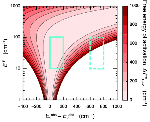
Figure 2 presents the free energy of activation, $\Delta F_{1\to 2}^{\ast}$, as a function of the reorganization energy, $E^{\rm R}=E_{1}^{\rm R}=E_{2}^{\rm R}$ and the absorption energy difference, $E_{1}^{\rm abs}-E_{2}^{\rm abs}$. For typical values of $0\leq E_{1}^{\rm abs}-E_{2}^{\rm abs}\leq 200\,\mathrm{cm^{-1}}$ and $10\,\mathrm{cm^{-1}}\leq E^{\rm R}\leq 100\,\mathrm{cm^{-1}}$, van Amerongen et al. (2000) the free energy of activation is very small in comparison to the thermal energy, $k_{\rm B}T\simeq 200\,\mathrm{cm^{-1}}$ at physiological temperature $T=300\,{\rm K}$. In other words, EET takes place in a practically activationless fashion. This clarifies the physical origin of ultrafast EET. In Figure 2 of Ref. Ishizaki and Fleming, 2009b, it is shown that the EET rate in the case of $E_{1}^{\rm abs}-E_{2}^{\rm abs}=100\,\mathrm{cm^{-1}}$ is maximized for values of the reorganization energy typical in natural light harvesting systems. This optimization is consistent with the activationless nature of the free-energy surface. In natural light harvesting systems, there is a manifold of states. Although the coordinates involved span multiple dimensions, this can be visualized as relaxation down a slightly “bumpy” funnel in a rather similar fashion to the Wolynes’ picture of protein folding landscapes. Bryngelson and Wolynes (1987) Furthermore, the barrierless nature of the energy transfer over the wide range of parameters typical in natural light harvesting systems means that inhomogeneous broadening has rather little influence on the dynamics. Similarly, there should be a very weak temperature dependence as observed, for example, in the LH2 complex of purple bacteria. Yang et al. (2001)

In the literature, the term of “coherent transfer” indicates that excitation travels as a quantum mechanical wave packet keeping its phase coherence; otherwise, the term of “incoherent transfer” is employed. As has been already discussed above, the incoherent “hopping” takes place from one minimum on the free-energy surface to another by overcoming a free-energy barrier that requires thermal activation. As demonstrated in eq (3.7) and Figure 2, however, the barrier is insignificantly small in comparison to the thermal energy when energy gaps of $\leq 200\,\mathrm{cm^{-1}}$ are considered, and thus the EET takes place in a nearly activationless fashion. Although this transfer process does not have coherent dynamics in the sense of the macroscopic ensemble, the transfer is still mainly driven by the electronic interaction between the pigments rather than by the thermal activation. The absence of long-lasting oscillatory transients in the ensemble average does not necessarily provide a correct insight into the microscopic nature of the EET dynamics.Ishizaki and Fleming (2011) Therefore, activationless EET needs to be distinguished from genuine incoherent “hopping” that requires thermal activation.

The current approach also has an implication regarding the importance of the initial excitation, either by pulsed coherent light, by incoherent thermal light such as sunlight, or by energy transfer. If the barrier for energy transfer is substantial, the initial condition is influenced accordingly. That is, on a bumpy free energy landscape with a free-energy well traps, the initial state would determine the course of the EET. However, if the process is barrierless, the sensitivity on the initial condition is greatly reduced.

The examination of the free energy of activation can also provide an insight into the necessity of a vibrational contribution to assist the EET. In the case that the free energy of activation does not exceed the thermal energy, the EET can take place easily without the assistance of vibrational modes, even though spectroscopic measurements may detect vibrational and vibronic signatures. This situation corresponds to the parameter region marked with the solid line box in Figure 2. Indeed, Ref. Fujihashi et al., 2015 demonstrated that the electronic-vibrational quantum mixtures do not necessarily play a significant role in EET dynamics in the FMO complex, despite contributing to the enhancement of long-lived quantum beating in 2D electronic spectra. In other photosynthetic pigment-protein complexes, however, relatively large differences among the absorption energies are found, e.g., in light harvesting complex II (LHCII),Novoderezhkin et al. (2005); Schlau-Cohen et al. (2009); Bhattacharyya and Fleming (2020); Arsenault et al. (2020) phycoerythrin 545, Collini et al. (2010); Kolli et al. (2012); O’Reilly and Olaya-Castro (2014) phycocyanin 645. Dean et al. (2016); Blau et al. (2018); Bennett et al. (2018) Hence, the parameter region marked with the dashed line box in Figure 2 was addressed, where $600\,\mathrm{cm^{-1}}\leq E_{1}^{\rm abs}-E_{2}^{\rm abs}\leq 800\,\mathrm{cm^{-1}}$ and $10\,\mathrm{cm^{-1}}\leq E^{\rm R}\leq 100\,\mathrm{cm^{-1}}$. In this region, the free energy of activation is high compared to the thermal energy at physiological temperatures.

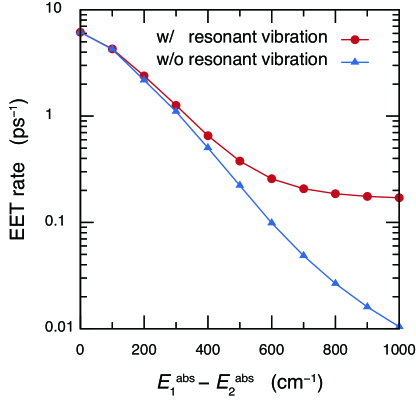
Some possible options for lowering the barrier with the fixed absorption energy difference are: (1) an increase in the environmental reorganization energy $E^{\rm R}$, (2) an increase in the inter-site electronic coupling $J_{mn}$, (3) correlated fluctuations in electronic energies,Lee et al. (2007); Ishizaki and Fleming (2010) or (4) assistance by vibrational modes. When the energy acceptor is a vibrationally excited state of pigment 2, the absorption energy difference is reduced to $E_{1}^{\rm abs}-(E_{2}^{\rm abs}+\hbar\omega_{\rm vib})$. In particular, the resonance between the vibrational frequency and the absorption energy difference leads to $E_{1}^{\rm abs}-(E_{2}^{\rm abs}+\hbar\omega_{\rm vib})=0$, and thus, the free-energy barrier in Figure 2 is substantially lowered. When the Condon approximation is valid for the transition dipole moments, the inter-pigment coupling is reduced as $J_{mn}\to-J_{mn}\mathrm{e}^{-S/2}\sqrt{S}$, with $S$ being the Huang-Rhys factor of the vibrational mode. Nevertheless, a substantial rate enhancement by a high-frequency vibrational mode is possible, as demonstrated in Figure 3. This is consistent with the recent theoretical result on vibrationally assisted EET in LHCII.Bhattacharyya and Fleming (2020) When the non-Condon effect is more prominent, the effect results in the enhancement of the vibronic transitions, Zhang et al. (2016) possibly leading to the further acceleration of the vibrationally assisted EET.Arsenault et al. (2020)

Figure 3 presents the EET rate influenced by a resonant vibrational mode whose frequency is a function of the absorption energy difference, $E_{1}^{\rm abs}-E_{2}^{\rm abs}$. Consistently with the insight gained from the free-energy barrier in Figure 2, the extent of the vibrational assistance increases with increasing the value of $E_{1}^{\rm abs}-E_{2}^{\rm abs}$. Here, it is noted that the vibrationally assisted EET rate exhibits a plateau in the region of $E_{1}^{\rm abs}-E_{2}^{\rm abs}>700\,\mathrm{cm^{-1}}$, indicating that the EET is promoted only by the vibrationally excited state. This can be also understood via the Förster rate formula. In the presence of a high-frequency vibrational mode, the absorption lineshape of pigment 2 is expressed as $A_{2}(\omega)=A_{2}^{(0)}(\omega)+A_{2}^{(1)}(\omega)+\dots$, where $A_{2}^{(v)}(\omega)$ is the lineshape associated with the optical transition to the $v$-th vibrational level in the electronically excited state and is approximately expressed as $A_{2}^{(v)}(\omega)\simeq({S^{v}}/{v!})A_{2}^{(0)}(\omega-v\omega_{\rm vib})$. In the case of high-frequency vibrational mode, the overlap between $A_{2}^{(0)}(\omega)$ and $A_{2}^{(1)}(\omega)$ vanishes, and hence, the vibrationally assisted EET rate is evaluated with the overlap integral between $F_{1}(\omega)$ and $A_{2}^{(1)}(\omega)=SA_{2}^{(0)}(\omega-\omega_{\rm vib})$. It should be noted that the overlap integral is independent of the value of $E_{1}^{\rm abs}-E_{2}^{\rm abs}$ under the condition of $E_{1}^{\rm abs}-E_{2}^{\rm abs}=\omega_{\rm vib}$.

References

- Brixner et al. (2005) T. Brixner, J. Stenger, H. M. Vaswani, M. Cho, R. E. Blankenship, and G. R. Fleming, Nature 434, 625 (2005).
- Cho et al. (2005) M. Cho, H. M. Vaswani, T. Brixner, J. Stenger, and G. R. Fleming, J. Phys. Chem. B 109, 10542 (2005).
- Engel et al. (2007) G. S. Engel, T. R. Calhoun, E. L. Read, T. K. Ahn, T. Mančal, Y.-C. Cheng, R. E. Blankenship, and G. R. Fleming, Nature 446, 782 (2007).
- Lee et al. (2007) H. Lee, Y.-C. Cheng, and G. R. Fleming, Science 316, 1462 (2007).
- Calhoun et al. (2009) T. R. Calhoun, N. S. Ginsberg, G. S. Schlau-Cohen, Y.-C. Cheng, M. Ballottari, R. Bassi, and G. R. Fleming, J. Phys. Chem. B 113, 16291 (2009).
- Savikhin et al. (1997) S. Savikhin, D. R. Buck, and W. S. Struve, Chem. Phys. 223, 303 (1997).
- Olaya-Castro et al. (2008) A. Olaya-Castro, C. Lee, F. Olsen, and N. Johnson, Phys. Rev. B 78, 085115 (2008).
- Mohseni et al. (2008) M. Mohseni, P. Rebentrost, S. Lloyd, and A. Aspuru-Guzik, J. Chem. Phys. 129, 174106 (2008).
- Plenio and Huelga (2008) M. B. Plenio and S. F. Huelga, New J. Phys. 10, 113019 (2008).
- Rebentrost et al. (2009) P. Rebentrost, M. Mohseni, I. Kassal, S. Lloyd, and A. Aspuru-Guzik, New J. Phys. 11, 033003 (2009).
- Ishizaki and Fleming (2009a) A. Ishizaki and G. R. Fleming, Proc. Natl. Acad. Sci. USA 106, 17255 (2009a).
- Nazir (2009) A. Nazir, Phys. Rev. Lett. 103, 146404 (2009).
- Caruso et al. (2009) F. Caruso, A. W. Chin, A. Datta, S. F. Huelga, and M. B. Plenio, J. Chem. Phys. 131, 105106 (2009).
- Panitchayangkoon et al. (2010) G. Panitchayangkoon, D. Hayes, K. A. Fransted, J. R. Caram, E. Harel, J. Wen, R. E. Blankenship, and G. S. Engel, Proc. Natl. Acad. Sci. USA 107, 12766 (2010).
- Collini et al. (2010) E. Collini, C. Y. Wong, K. E. Wilk, P. M. G. Curmi, P. Brumer, and G. D. Scholes, Nature 463, 644 (2010).
- Caruso et al. (2010) F. Caruso, A. W. Chin, A. Datta, S. F. Huelga, and M. B. Plenio, Phys. Rev. A 81, 062346 (2010).
- Sarovar et al. (2010) M. Sarovar, A. Ishizaki, G. R. Fleming, and K. B. Whaley, Nat. Phys. 6, 462 (2010).
- Ishizaki and Fleming (2010) A. Ishizaki and G. R. Fleming, New J. Phys. 12, 055004 (2010).
- Hoyer et al. (2010) S. Hoyer, M. Sarovar, and K. Birgitta Whaley, New J. Phys. 12, 065041 (2010).
- Fassioli et al. (2010) F. Fassioli, A. Nazir, and A. Olaya-Castro, J. Phys. Chem. Lett. 1, 2139 (2010).
- Abramavicius and Mukamel (2010) D. Abramavicius and S. Mukamel, J. Chem. Phys. 133, 064510 (2010).
- Panitchayangkoon et al. (2011) G. Panitchayangkoon, D. V. Voronine, D. Abramavicius, J. R. Caram, N. H. C. Lewis, S. Mukamel, and G. S. Engel, Proc. Natl. Acad. Sci. USA 108, 20908 (2011).
- Scholak et al. (2011) T. Scholak, F. de Melo, T. Wellens, F. Mintert, and A. Buchleitner, Phys. Rev. E 83, 021912 (2011).
- Schlau-Cohen et al. (2012) G. S. Schlau-Cohen, A. Ishizaki, T. R. Calhoun, N. S. Ginsberg, M. Ballottari, R. Bassi, and G. R. Fleming, Nat. Chem. 4, 389 (2012).
- Lewis and Ogilvie (2012) K. L. M. Lewis and J. P. Ogilvie, J. Phys. Chem. Lett. 3, 503 (2012).
- Westenhoff et al. (2012) S. Westenhoff, D. Palec̆ek, P. Edlund, P. Smith, and D. Zigmantas, J. Am. Chem. Soc. 134, 16484 (2012).
- Dawlaty et al. (2012) J. M. Dawlaty, A. Ishizaki, A. K. De, and G. R. Fleming, Phil. Trans. R. Soc. A 370, 3672 (2012).
- Chang and Cheng (2012) H.-T. Chang and Y.-C. Cheng, J. Chem. Phys. 137, 165103 (2012).
- Hoyer et al. (2012) S. Hoyer, A. Ishizaki, and K. B. Whaley, Phys. Rev. E 86, 041911 (2012).
- Shabani et al. (2012) A. Shabani, M. Mohseni, H. Rabitz, and S. Lloyd, Phys. Rev. E 86, 011915 (2012).
- Wu et al. (2012) J. Wu, F. Liu, J. Ma, R. J. Silbey, and J. Cao, J. Chem. Phys. 137, 174111 (2012).
- Dijkstra and Tanimura (2012) A. G. Dijkstra and Y. Tanimura, New J. Phys. 14, 073027 (2012).
- Hildner et al. (2013) R. Hildner, D. Brinks, J. B. Nieder, R. J. Cogdell, and N. F. van Hulst, Science 340, 1448 (2013).
- Chin et al. (2013) A. W. Chin, S. F. Huelga, and M. B. Plenio, Nat. Phys. 9, 113 (2013).
- Gelzinis et al. (2013) A. Gelzinis, L. Valkunas, F. D. Fuller, J. P. Ogilvie, S. Mukamel, and D. Abramavicius, New J. Phys. 15, 075013 (2013).
- Rivera et al. (2013) E. Rivera, D. Montemayor, M. Masia, and D. F. Coker, J. Phys. Chem. B 117, 5510 (2013).
- O’Reilly and Olaya-Castro (2014) E. J. O’Reilly and A. Olaya-Castro, Nat. Commun. 5, 1 (2014).
- De et al. (2014) A. K. De, D. Monahan, J. M. Dawlaty, and G. R. Fleming, J. Chem. Phys. 140, 194201 (2014).
- Dijkstra and Tanimura (2015) A. G. Dijkstra and Y. Tanimura, J. Chem. Phys. 142, 212423 (2015).
- Scholes et al. (2017) G. D. Scholes, G. R. Fleming, L. X. Chen, A. Aspuru-Guzik, A. Buchleitner, D. F. Coker, G. S. Engel, R. van Grondelle, A. Ishizaki, D. M. Jonas, et al., Nature 543, 647 (2017).
- Knee et al. (2017) G. C. Knee, P. Rowe, L. D. Smith, A. Troisi, and A. Datta, J. Phys. Chem. Lett. 8, 2328 (2017).
- Dutta and Bagchi (2017) R. Dutta and B. Bagchi, J Phys Chem Lett 8, 5566 (2017).
- Sakamoto and Tanimura (2017) S. Sakamoto and Y. Tanimura, J. Phys. Chem. Lett. 8, 5390 (2017).
- Thyrhaug et al. (2018) E. Thyrhaug, R. Tempelaar, M. J. P. Alcocer, K. Žídek, D. Bína, J. Knoester, T. L. C. Jansen, and D. Zigmantas, Nature Chemistry 10, 780 (2018).
- Saito et al. (2019) S. Saito, M. Higashi, and G. R. Fleming, J. Phys. Chem. B 123, 9762 (2019).
- Kim et al. (2019) C. W. Kim, W.-G. Lee, I. Kim, and Y. M. Rhee, J. Phys. Chem. A 123, 1186 (2019).
- Muñoz and Schlawin (2020) C. S. Muñoz and F. Schlawin, Phys. Rev. Lett. 124, 203601 (2020).
- Cao et al. (2020) J. Cao, R. J. Cogdell, D. F. Coker, H.-G. Duan, J. Hauer, U. Kleinekathoefer, T. L. C. Jansen, T. Mančal, R. J. D. Miller, J. P. Ogilvie, et al., Science Advances 6, eaaz4888 (2020).
- Chan et al. (2013) W.-L. Chan, T. C. Berkelbach, M. R. Provorse, N. R. Monahan, J. R. Tritsch, M. S. Hybertsen, D. R. Reichman, J. Gao, and X. Y. Zhu, Acc. Chem. Res. 46, 1321 (2013).
- Gélinas et al. (2014) S. Gélinas, A. Rao, A. Kumar, S. L. Smith, A. W. Chin, J. Clark, T. S. van der Poll, G. C. Bazan, and R. H. Friend, Science 343, 512 (2014).
- Lee et al. (2015) M. H. Lee, J. Aragó, and A. Troisi, J. Phys. Chem. C 119, 14989 (2015).
- Bredas et al. (2016) J.-L. Bredas, E. H. Sargent, and G. D. Scholes, Nat. Mater. 16, 35 (2016).
- Kato and Ishizaki (2018) A. Kato and A. Ishizaki, Phys. Rev. Lett. 121, 026001 (2018).
- Nemeth et al. (2010) A. Nemeth, F. Milota, T. Mančal, V. Lukeš, J. Hauer, H. F. Kauffmann, and J. Sperling, J. Chem. Phys. 132, 184514 (2010).
- Mančal et al. (2010) T. Mančal, A. Nemeth, F. Milota, V. Lukeš, H. F. Kauffmann, and J. Sperling, J. Chem. Phys. 132, 184515 (2010).
- Butkus et al. (2012) V. Butkus, D. Zigmantas, L. Valkunas, and D. Abramavicius, Chem. Phys. Lett. 545, 40 (2012).
- Yuen-Zhou et al. (2012) J. Yuen-Zhou, J. J. Krich, and A. Aspuru-Guzik, J. Chem. Phys. 136, 234501 (2012).
- Caycedo-Soler et al. (2012) F. Caycedo-Soler, A. W. Chin, J. Almeida, S. F. Huelga, and M. B. Plenio, J. Chem. Phys. 136, 155102 (2012).
- Christensson et al. (2012) N. Christensson, H. F. Kauffmann, T. Pullerits, and T. Mančal, J. Phys. Chem. B 116, 7449 (2012).
- Tiwari et al. (2013) V. Tiwari, W. K. Peters, and D. M. Jonas, Proc. Natl. Acad. Sci. USA 110, 1203 (2013).
- Romero et al. (2014) E. Romero, R. Augulis, V. I. Novoderezhkin, M. Ferretti, J. Thieme, D. Zigmantas, and R. van Grondelle, Nat. Phys. 10, 677 (2014).
- Fuller et al. (2014) F. D. Fuller, J. Pan, A. Gelzinis, V. Butkus, S. S. Senlik, D. E. Wilcox, C. F. Yocum, L. Valkunas, D. Abramavicius, and J. P. Ogilvie, Nat. Chem. 6, 706 (2014).
- Fujihashi et al. (2015) Y. Fujihashi, G. R. Fleming, and A. Ishizaki, J. Chem. Phys. 142, 212403 (2015).
- Monahan et al. (2015) D. M. Monahan, L. Whaley-Mayda, A. Ishizaki, and G. R. Fleming, J. Chem. Phys. 143, 065101 (2015).
- Fujihashi et al. (2016) Y. Fujihashi, G. R. Fleming, and A. Ishizaki, J. Chin. Chem. Soc. 63, 49 (2016).
- Fujihashi et al. (2018) Y. Fujihashi, M. Higashi, and A. Ishizaki, J. Phys. Chem. Lett. 9, 4921 (2018).
- Jang et al. (2008) S. Jang, Y.-C. Cheng, D. R. Reichman, and J. D. Eaves, J. Chem. Phys. 129, 101104 (2008).
- Ishizaki and Fleming (2009b) A. Ishizaki and G. R. Fleming, J. Chem. Phys. 130, 234111 (2009b).
- Prior et al. (2010) J. Prior, A. W. Chin, S. F. Huelga, and M. B. Plenio, Phys. Rev. Lett. 105, 050404 (2010).
- Huo and Coker (2010) P. Huo and D. F. Coker, J. Chem. Phys. 133, 184108 (2010).
- Tao and Miller (2010) G. Tao and W. H. Miller, J. Phys. Chem. Lett. 1, 891 (2010).
- Kelly and Rhee (2011) A. Kelly and Y. M. Rhee, J. Phys. Chem. Lett. 2, 808 (2011).
- Nalbach et al. (2011) P. Nalbach, A. Ishizaki, G. R. Fleming, and M. Thorwart, New J. Phys. 13, 063040 (2011).
- Berkelbach et al. (2012) T. C. Berkelbach, T. E. Markland, and D. R. Reichman, J. Chem. Phys. 136, 084104 (2012).
- Kelly and Markland (2013) A. Kelly and T. E. Markland, J. Chem. Phys. 139, 014104 (2013).
- Banchi et al. (2013) L. Banchi, G. Costagliola, A. Ishizaki, and P. Giorda, J. Chem. Phys. 138, 184107 (2013).
- Jang et al. (2014) S. Jang, S. Hoyer, G. R. Fleming, and K. B. Whaley, Phys. Rev. Lett. 113, 188102 (2014).
- Hwang-Fu et al. (2015) Y.-H. Hwang-Fu, W. Chen, and Y.-C. Cheng, Chem. Phys. 447, 46 (2015).
- Tamascelli et al. (2019) D. Tamascelli, A. Smirne, J. Lim, S. F. Huelga, and M. B. Plenio, Phys. Rev. Lett. 123, 090402 (2019).
- Adolphs and Renger (2006) J. Adolphs and T. Renger, Biophys. J. 91, 2778 (2006).
- Kubo et al. (1985) R. Kubo, M. Toda, and N. Hashitsume, Statistical Physics II (Springer, Berlin, Heidelberg, 1985).
- Marchi et al. (1993) M. Marchi, J. N. Gehlen, D. Chandler, and M. Newton, J. Am. Chem. Soc. 115, 4178 (1993).
- Chandler (1998) D. Chandler, in Classical and Quantum Dynamics in Condensed Phase Simulations, edited by B. J. Berne, G. Ciccotti, and D. F. Coker (World Scientific, Singapore, 1998), pp. 25–49.
- Ishizaki et al. (2010) A. Ishizaki, T. R. Calhoun, G. S. Schlau-Cohen, and G. R. Fleming, Phys. Chem. Chem. Phys. 12, 7319 (2010).
- van Amerongen et al. (2000) H. van Amerongen, L. Valkunas, and R. van Grondelle, Photosynthetic excitons (World Scientific, Singapore, 2000).
- Marcus (1993) R. A. Marcus, Rev. Mod. Phys. 65, 599 (1993).
- Bryngelson and Wolynes (1987) J. D. Bryngelson and P. G. Wolynes, Proc. Natl. Acad. Sci. USA 84, 7524 (1987).
- Yang et al. (2001) M. Yang, R. Agarwal, and G. R. Fleming, J. Photochem. Photobiol. A 142, 107 (2001).
- Ishizaki and Fleming (2011) A. Ishizaki and G. R. Fleming, J. Phys. Chem. B 115, 6227 (2011).
- Novoderezhkin et al. (2005) V. I. Novoderezhkin, M. A. Palacios, H. van Amerongen, and R. van Grondelle, J. Phys. Chem. B 109, 10493 (2005).
- Schlau-Cohen et al. (2009) G. S. Schlau-Cohen, T. R. Calhoun, N. S. Ginsberg, E. L. Read, M. Ballottari, R. Bassi, R. van Grondelle, and G. R. Fleming, J. Phys. Chem. B 113, 15352 (2009).
- Bhattacharyya and Fleming (2020) P. Bhattacharyya and G. R. Fleming, J. Chem. Phys. 153, 044119 (2020).
- Arsenault et al. (2020) E. A. Arsenault, Y. Yoneda, M. Iwai, K. K. Niyogi, and G. R. Fleming, Nat. Commun. 11, 1 (2020).
- Kolli et al. (2012) A. Kolli, E. J. O’Reilly, G. D. Scholes, and A. Olaya-Castro, J. Chem. Phys. 137, 174109 (2012).
- Dean et al. (2016) J. C. Dean, T. Mirkovic, Z. S. D. Toa, D. G. Oblinsky, and G. D. Scholes, Chem 1, 858 (2016).
- Blau et al. (2018) S. M. Blau, D. I. G. Bennett, C. Kreisbeck, G. D. Scholes, and A. Aspuru-Guzik, Proc. Natl. Acad. Sci. U.S.A. 115, E3342 (2018).
- Bennett et al. (2018) D. I. G. Bennett, P. Malý, C. Kreisbeck, R. van Grondelle, and A. Aspuru-Guzik, J Phys Chem Lett 9, 2665 (2018).
- Zhang et al. (2016) H.-D. Zhang, Q. Qiao, R.-X. Xu, and Y. Yan, J. Chem. Phys. 145, 204109 (2016).
- Brumer and Shapiro (2012) P. Brumer and M. Shapiro, Proc. Natl. Acad. Sci. USA 109, 19575 (2012).
- Mančal and Valkunas (2010) T. Mančal and L. Valkunas, New J. Phys. 12, 065044 (2010).
- Fassioli et al. (2012) F. Fassioli, A. Olaya-Castro, and G. D. Scholes, J. Phys. Chem. Lett. 3, 3136 (2012).
- Pachón et al. (2017) L. A. Pachón, J. D. Botero, and P. Brumer, J. Phys. B.: At. Mol. Opt. Phys. 50, 184003 (2017).
- Blankenship (2013) R. E. Blankenship, Molecular Mechanisms of Photosynthesis (Wiley Blackwell, West Sussex, 2013).
- Chan et al. (2018) H. C. H. Chan, O. E. Gamel, G. R. Fleming, and K. B. Whaley, J. Phys. B: At. Mol. Opt. Phys. 51 (2018).
- Deng et al. (2019) Y.-H. Deng, H. Wang, X. Ding, Z. C. Duan, J. Qin, M. C. Chen, Y. He, Y.-M. He, J.-P. Li, Y.-H. Li, et al., Phys. Rev. Lett. 123, 080401 (2019).
- Fujihashi et al. (2020) Y. Fujihashi, R. Shimizu, and A. Ishizaki, Phys. Rev. Research 2, 023256 (2020).