Instability of steady-state mixed-state symmetry-protected topological order to strong-to-weak spontaneous symmetry breaking
Abstract
Recent experimental progress in controlling open quantum systems enables the pursuit of mixed-state nonequilibrium quantum phases. We investigate whether open quantum systems hosting mixed-state symmetry-protected topological states as steady states retain this property under symmetric perturbations. Focusing on the decohered cluster state—a mixed-state symmetry-protected topological state protected by a combined strong and weak symmetry—we construct a parent Lindbladian that hosts it as a steady state. This Lindbladian can be mapped onto exactly solvable reaction-diffusion dynamics, even in the presence of certain perturbations, allowing us to solve the parent Lindbladian in detail and reveal previously-unknown steady states. Using both analytical and numerical methods, we find that typical symmetric perturbations cause strong-to-weak spontaneous symmetry breaking at arbitrarily small perturbations, destabilize the steady-state mixed-state symmetry-protected topological order. However, when perturbations introduce only weak symmetry defects, the steady-state mixed-state symmetry-protected topological order remains stable. Additionally, we construct a quantum channel which replicates the essential physics of the Lindbladian and can be efficiently simulated using only Clifford gates, Pauli measurements, and feedback.
I Introduction
Dissipation is typically viewed as detrimental to quantum information, but recent advances in experimental control have begun to harness its potential to create well-controlled nontrivial open quantum systems [1, 2, 3, 4, 5, 6, 7]. This raises an intriguing question: can an open quantum system host exotic quantum phases that are inherently mixed and nonthermal [8]? Namely, are there phases that cannot be understood within the typical equilibrium framework, where the phases are described by either a pure state or a Gibbs thermal state? This question becomes particularly compelling if the mixed-state phase leads to a degenerate steady-state manifold, offering potential for classical or quantum memory [9, 10, 11, 12, 13, 14]. In such cases, the stability of the phase would ensure the preservation of the degeneracy.
Recently, mixed-state symmetry-protected topological (SPT) states [15, 16, 17, 18, 19, 20, 21, 22, 23, 24, 25, 26, 27] have emerged as promising candidates for inherently mixed-state phases. Mixed-state SPT phases consist of short-range entangled density matrices which cannot be connected to density matrices in other phases by symmetric two-way dissipative evolution [8]. The related topics of anomaly [28, 29, 30] and intrinsic topological order [31, 32, 33] in mixed states have also been investigated in several recent works. Tensor network descriptions of mixed-state SPTs have also been used recently [34, 19, 23].
When considering open quantum systems or density matrices, the notion of symmetry is augmented compared to the pure state setting, which leads to two types of symmetries [35, 36, 12, 13]. Specifically, if the density matrix needs to be conjugated by a unitary of a symmetry group from both the ket and the bra sides to get back the same density matrix, then the symmetry is called a weak symmetry. On the other hand, if we can also get back the density matrix by applying different unitaries on the ket and the bra sides, then the symmetry is called a strong symmetry. As pointed out in Refs. [8, 37], there are no nontrivial mixed-state SPT phases if only weak symmetry is imposed. However, a mixed state can exhibit SPT order if the imposed symmetry is strong, although this order is is captured by some pure-state SPT phase. The aforementioned mixed-state SPT order, requiring a combination of strong and weak symmetry, provides an opportunity for an inherently mixed-state phase.
The distinction between strong and weak symmetries also introduces a novel type of spontaneous symmetry breaking unique to open quantum systems, where the strong symmetry is spontaneously broken down to weak symmetry, dubbed strong-to-weak spontaneous symmetry breaking (SW-SSB) [27, 38, 39]. Detecting SW-SSB requires measuring quantities that are nonlinear in the density matrix, a task achievable in quantum devices but not in conventional condensed-matter systems. It has been suggested that a spontaneously broken strong symmetry can lead to a degenerate steady-state manifold [13], which implies that it should be interesting to explore the steady-state manifold of SW-SSB.
Most studies on mixed-state phases, including mixed-state SPT order and SW-SSB, have focused on the “quasilocal finite-depth quantum channel” framework [8], akin to that used for defining gapped phases of ground states of closed systems [40, 41]. However, given the interest in potential steady-state degeneracy in mixed-state phases, our work focuses on the steady-state phase of an open quantum system. Finding the steady states of an open quantum system can be mapped to finding extremal eigenstates of a non-Hermitian superoperator. Since ground states are extremal eigenstates of a Hamiltonian, the steady-state phase viewpoint provides a different analogy. While in the gapped ground-state scenario, the “quasilocal finite-depth quantum circuit” and “gapped ground-state phase” definitions are two sides of the same coin, the relationship between the “quasilocal finite-depth quantum channel” and “steady-state phase” is unclear. Our focus on the “steady-state phase” perspective therefore complements previous works.
Motivated by these considerations, we investigate the stability of mixed-state SPT order of steady-state phases of open quantum systems, using the decohered cluster state—a simple mixed-state SPT order protected by a combined strong and weak symmetry [15]—as a test bed. We first employ the matrix product density operator representation to analyze its mixed-state SPT order characteristics, such as bulk-edge correspondence, nontrivial string order, and edge states. We then construct a parent Lindbladian that hosts the decohered cluster state as a steady state with the required symmetry.
Similar to the pure cluster state [42, 43], the decohered cluster state can be disentangled by a depth-two circuit of controlled-Z gates, yielding the corresponding trivial mixed-state SPT order. This duality allows us to map the open system dynamics to an exactly solvable reaction-diffusion model [44], enabling a thorough analysis of the Lindbladian, including the degeneracy of the steady-state manifold, previously unknown steady states, and the mixing time of the system.
We also study an interpolation between the parent Lindbladian of the decohered cluster state and that of the trivial mixed-state SPT order, analogous to the pure-state case [45, 46]. Surprisingly, we find that the steady states at any point in this interpolation are neither nontrivial mixed-state SPT nor trivial mixed-state SPT orders. Instead, they exhibit SW-SSB, which destroys the mixed-state SPT order. The mapping to the reaction-diffusion model suggests that the proliferation of point-like defects affecting the strong symmetry destroys the mixed-state SPT order, leading to SW-SSB, which is typical for symmetric perturbations. However, for perturbations that only affect weak symmetry, the mixed-state SPT order and its associate steady-state degeneracy remain stable. Finally, we propose a quantum channel-based dynamics that replicates the essential physics of our findings. We are able to classically simulate this channel efficiently since it consists of Clifford gates, Pauli measurements, and feedback [47].
The structure of the paper is as follows. In Section˜II, we introduce the decohered cluster state and describe its classification and characteristics, aided by tensor network representations. In Section˜III, we construct a parent Lindbladian which hosts the state we introduced in Section˜II as a steady state, and solve for the full spectrum of the parent Lindbladian, including all of the steady states, by mapping to an exactly solvable Lindbladian. In Section˜IV, we consider different types of perturbations to the parent Lindbladian and analyze the resulting steady states numerically via density matrix renormalization group (DMRG) and analytics, where possible. We find that the mixed-state SPT order of the steady state is unstable to SW-SSB for a wide class of symmetric perturbations to the Lindbladian. In Section˜V, we consider a quantum channel which replicates the essential physics of the parent and perturbed Lindbladians and admits efficient Clifford simulation. We summarize the paper and give an outlook in Section˜VI.
II Decohered cluster state
We begin by introducing the “decohered cluster state” [15], a certain type of cluster state in the presence of decoherence. We review its symmetries and classification within the framework of mixed-state SPT phases as discussed in Refs. [8, 15, 16]. Using tensor network diagrammatics or matrix product density operators, we show that the decohered cluster state exhibits non-trivial string order and bulk-edge correspondence.
II.1 Cluster state and decoherence
The well-known pure cluster state on a closed chain of qubits [42] can be expressed as
| (1) |
where
| (2) |
are decorated domain wall states [48]. Here, we define () to be the eigenstates of () with eigenvalues . Note that we denote the eigenstates of with eigenvalues by in this paper. The decorated domain wall states are constructed by first specifying a configuration which determines the charge on the odd sites, and then “decorating” each domain wall with a state charged under . More specifically, when , the interceding even site is fixed to , and to otherwise.
The decohered cluster state is defined by taking the equal-weight incoherent mixture of the decorated domain wall states shown in Eq.˜3, rather than their coherent superposition. Defined on a closed chain of qubits, the decohered cluster state reads [15]
| (3) |
As we will see later, it is exhibits nontrivial mixed-state SPT order.
II.2 Symmetry
We hereby discuss the notions of weak and strong symmetry applicable to mixed states [35, 36, 12, 13]. In particular, a weakly -symmetric matrix satisfies for all , where is an Abelian symmetry group and . On the other hand, a strongly -symmetric matrix satisfies and for all , where , . When is Hermitian, .
Consider the following operators in the Hilbert space of qubits on a closed ring,
| (4) |
The decohered cluster state is a mixed-state SPT order under the direct product of a strong symmetry and a weak symmetry, as classified in Refs. [15, 16], where the strong symmetry (denoted as from now on) is generated by , while the weak symmetry (denoted as from now on) is generated by . We will use , , and (with argument suppressed) when we are referring to the charges under the strong symmetry and weak symmetry .
For the decohered cluster state defined in Eq. (3), we find that and , so that lies in the symmetry sector. There is an intuitive way to understand why acts as a weak symmetry while acts as a strong symmetry. Note that counts the parity of the number of domain walls in each decorated domain wall state. With periodic boundary conditions, the system’s topology enforces an even number of domain walls in every state, . This will be the case for both the bra states and the ket states in . We therefore see that must be strongly symmetric with . On the other hand, acts on the decorated domain wall states as , where . This transformation is only a symmetry if it acts simultaneously from both the bra and the ket sides, indicating that can only be a weak symmetry.
II.3 Classification as a mixed-state phase
One physically motivated approach to define mixed-state phases is to define an equivalence class relation among the states, where the equivalence is defined by a short-time physical processes. This mimics the definition of ground states being in the same phase if they can be adiabatically perturbed to each other rapidly. This definition was put forward by Ref. [8], and we review their definition more rigorously in Appendix˜A. Informally, it states that for two mixed states and to be in the same phase, there has to exist two time-independent, symmetric geometrically local Lindbladians and such that and are small, where is some short time (“fast-driven”) and where is the trace distance. Note that the smallness of the trace distance implies the closeness of all the observables between and , i.e., by Hölder’s inequality, where is the operator norm. Furthermore, this “fast-driven” condition implies stability of local observables to local perturbations in the Lindbladian terms [49, 8, 50].
One can also define the equivalence-class relation through quantum channels, analogous to the Lindbladian equivalence-class relation. That is, if there exist two symmetric finite-depth local quantum channels [15, 16] and such that and are small, then we say and are in the same phase. Note that in both the Lindbladian and quantum channel equivalence-class relations, the bi-directional “fast-driven” condition is important, as the Lindbladian evolution and the quantum channel are usually not reversible.
Building on the quantum-channel equivalence-class relation, Refs. [15, 16] show that if the strong-string order parameter (an order parameter used to diagnose SPT orders, see Section˜II.5) in the state is zero, then there does not exist a symmetric finite-depth channel such that the string order parameter of is of order one. That is to say, if has a string order parameter of order one, then can never be small. We know from Refs. [15, 16] that has a nonzero string order parameter (see also Section˜II.5 for more explanation on this). Thus, is in a nontrivial mixed-state SPT order protected by , as stated in Refs. [15, 16].
Here, we complement the above result by showing that has nontrivial SPT order protected by symmetry under the Lindbladian equivalence-class relation as well. Using Lieb-Robinson bounds [51, 52], we show that can never be small for a symmetric Lindbladian within some short time . The detailed statement and its proof are presented in Appendix˜A.
The above results can be interpreted as follows—the nontrivial SPT order of is hard to build, which forbids a “fast-driven” symmetric Lindbladian or a symmetric finite-depth quantum channel from bringing a trivial state close to , which is a nontrivial SPT state. On the other hand, it is interesting to know if can be brought close to a trivial state in a short time or in a short depth. In Appendix˜B, we show that the string order parameter corresponding to the symmetry defined in Eq. (4) is easy to destroy. In particular, we show that a simple trace channel and the corresponding trace Lindbladian can destroy the string order in depth one and in a short time, respectively. Interestingly, the destruction of the string order is accompanied by the “strong-to-weak” spontaneous symmetry breaking, which has received a lot of attention recently [27, 38, 39].
II.4 Tensor network representation
It is instructive to express as a matrix product density operator, as it helps us expose the edge modes on an open chain, extract the projective representation, and calculate the string order parameters. We first define two families of matrices in the virtual space spanned by and . These matrices are two-index tensors given by and , where . We can then define two four-index tensors:
| (5) | ||||
| (6) | ||||
where are the physical indices, are the virtual indices, and as above and . Abbreviating the configuration , we can then write , where
| (7) | ||||
The sums over and in the definition of each go over all possibilities, while the restriction to decorated domain wall states is taken care of by the coefficients . Pictorially, we write
| (8) | ||||
where we have used periodic boundary conditions. When tensors appear without indices explicitly denoted, we assume they are summed over with the corresponding bras and kets.
It is worth noting that the tensors defined in Eqs.˜5 and 6 have the following “pulling-through” relations:
| (9a) | |||
| (9b) | |||
| (9c) |
| (9d) |
Using these relations, it will be easy to show that the symmetry forms a projective representation on the virtual space.
Let us briefly review the relationship between SPT order in 1d and projective representations. Pure-state SPT phases in 1d protected by a global symmetry are characterized and classified by edge modes transforming in a projective representation of . The classification can be formulated in terms of the second cohomology group , which tabulates the inequivalent projective representations of with phases. In Ref. [15], it was shown that mixed-state SPT phases protected by a combination of a strong symmetry and weak symmetry are classified by . In the present case of the decohered cluster state, we have , so that the above classification evaluates to . This means that there is a single nontrivial mixed-state SPT phase with symmetry , with respect to the definition given in Ref. [15]. And indeed a nontrivial SPT order can be constructed from the domain-wall construction between the strong and the weak symmetries such as .
To see that the decohered cluster state indeed realizes the symmetry projectively at its boundary, we first construct the following family of density matrices on open boundary conditions:
| (10) |
where , and . The states in Eq.˜10 span a 4-dimensional linear space with complex coefficients, where the physical density matrices correspond to the subspace of Hermitian matrices with unit trace. This space can encode two classical bits of information.
We then act with the symmetry operators on . Akin to the pure state case, we see via the pulling-through relations Eq.˜9 that the global symmetry factors to a product of operators acting on each virtual edge state:
We have found that the symmetries reduce to an effective action on the edge Hilbert space, namely
| (11) | ||||
As in the pure state case, these operators commute globally, but anti-commute if either edge is taken in isolation:
| (12) |
The matrices and obtained by pulling the symmetry to each edge generate the algebra , which forms a projective representation of the group . This is precisely what we mean by the statement that the symmetry is realized projectively at the edge.
II.5 String order parameters
While conventional SPT orders do not spontaneously break symmetry and therefore do not admit local order parameters, they can be characterized by non-local string order parameters [53, 54, 55, 56, 57]. Importantly, the diagnostic of an SPT order is done by the “patterns of zeros” of various string order parameters [55]. We here briefly review the definition of a string order parameter in the pure state case. Suppose we have an Abelian on-site symmetry with symmetry operators
| (13) |
In general, a string order parameter that detects a nontrivial projective representation of the symmetry consists of a finite string of operators in a region with operators appended to the left and right ends of the string which transform under conjugate irreps and of the other symmetry,
| (16) |
The string operators let us define the string order parameter for a pure state , which is simply .
One natural generalization of the string order parameter from pure states to mixed states is to measure the expectation value of the strong-string operator (defined below) in the state :
| (17) |
where
| (18) |
for odd and . The Roman numeral I appearing in the subscript indicates that the correlator is linear in the density matrix (i.e. Rényi-1), and distinguishes it from other correlators which we will define shortly which are quadratic in the density matrix. This definition has been used in prior works, and it has been shown that it is an order parameter for the mixed-state SPT order [16]. If we try to define an analogous order parameter for the weak-string operator , then we find that it is trivially one because the weak-string operator acts from both the ket and the bra sides and , more specifically .
One way of generating a useful string correlator corresponding to the weak symmetry is to map density matrices to vectors in a doubled Hilbert space with twice the number of qubits and consider the string correlators in this doubled space [27]. The mapping of density matrices to vectors in the doubled Hilbert space is as follows:
| (19) |
where the subscripts and denote the left and the right Hilbert spaces and and denote some computational basis.
In the doubled Hilbert space, the symmetry operators become , for the strong ket and the strong bra symmetries, and for the weak symmetry. Here the first factor of the tensor product acts on the left (ket) Hilbert space and the second factor acts on the right (bra) Hilbert space. We denote the expectation values of an operator in the doubled Hilbert space by
| (20) |
where is a superoperator that corresponds to the operator in the doubled Hilbert space. For example, .
Now, by substituting the various symmetry operators in the definition of the string operator, Eq.˜16, we find the various string correlators that we need. If on the even sites, and the end point operators are on the odd sites and , then we get the following correlator which we call the Rényi-2 strong string correlator:
| (21) |
where is defined as in Eq.˜18 and the Roman numeral II reflects the fact that the correlator is quadratic in the density matrix, or Rényi-2. Note that . Thus this choice of the end-point operators can in principle be used to detect nontrivial SPT order.
If we take the symmetry to be the weak symmetry in Eq.˜16, that is, on the odd sites, and the end-point operators on the even sites and , then we get the Rényi-2 weak string correlator:
| (22) |
where as defined earlier. Note that .
Next, we construct two more correlators by taking the end point operators to be . These are the Rényi-2 trivial strong-string correlator and the Rényi-2 trivial weak-string correlator:
| (23) |
where has the strong symmetry operators in the bulk and as the end point operators with restricted to be odd, while has the weak symmetry operators in the bulk and as the end point operators with restricted to be even.
While for a generic density matrix, the Rényi-1 and Rényi-2 type of correlators are independent, Ref. [27] shows that they are related to each other if the state is short-range entangled. The patterns of zeros used to diagnose trivial and nontrivial SPT orders are summarized in Table 3.
Now we show, using tensor network diagrams, that for in the state . Acting on with each of the string operators, we find
Because is invariant under the action of the strings, the string order parameters will be identically one whether we chose to contract the physical legs of according to the Rényi-1 or Rényi-2 conventions.
III Parent Lindbladian
In the study of quantum phases of pure states, we traditionally begin with a Hamiltonian that depends on a set of parameters. Quantum phases are then understood to be finite volumes of Hamiltonian parameter space in which the ground state(s) of the Hamiltonian display qualitatively similar features, such as long-range order and degeneracy. These features can be diagnosed by measuring local and/or nonlocal order parameters whose values stratify Hamiltonian parameter space into distinct phases. In an effort to generalize this perspective to the mixed state case, we will construct a parent Lindbladian for the decohered cluster state and map out the phase diagram in its vicinity by measuring local and nonlocal order parameters.
If a Hamiltonian is in a nontrivial SPT phase, then it is known that the phase is stable to symmetric perturbations. Specifically, if one adds a symmetric perturbation to the Hamiltonian, then the ground state degeneracy does not change (in the thermodynamic limit) and ground states of the perturbed Hamiltonian will have a nonzero string order parameter, reflecting a nontrivial projective representation. Our aim in this section is to test if this analogy carries over to mixed states and Lindbladians. We construct a local Lindbladian whose steady state is the decohered cluster state . We then add symmetric local Lindbladian perturbations and study the properties of the new steady states. This raises the questions of whether there is a way of defining mixed state phases of matter which focuses on parent Lindbladians rather than density matrices, and whether this perspective reveals anything new. Toward this aim, we will construct a -symmetric parent Lindbladian which hosts as a NESS, i.e. .
III.1 The model
We define the parent Lindbladian on an open chain of qubits labelled by as follows:
| (24) |
where denotes the standard Lindblad dissipator for a jump operator [58, 59]. For periodic boundary conditions, we add the terms and for to Section˜III.1, where the site label . The jump operators are
| (25a) | |||
| (25b) | |||
| (25c) |
Since all the jump operators commute with , the Lindbladian has the symmetry, while it is easy to check that renders the symmetry weak. Thus, our parent Lindbladian has the symmetry introduced in Section˜II.2. Each of the terms , , plays a distinct role in driving an arbitrary density matrix in the same symmetry sector as to the steady state .
The jump operators have the following physical meanings. for even is designed to stabilize the domain-wall configurations. If the configuration is violated, we have , and we fix the configuration by applying . Note that this configuration can also be fixed by applying , , , etc. However, applying is forbidden as it breaks the strong symmetry ; we choose to apply because the resulting jump operator has the lowest weight. Now within the domain-wall configuration space, is designed to decohere the “off-diagonal” domain-wall configurations, leaving only , while makes the probability of getting all the configurations equal.
Note that is a steady state for any values of the rates of the jump operators, but we will choose these rates to be equal. We have verified that changing the rates does not change the physics qualitatively.
Recall that the decohered cluster state is a mixed-state SPT state protected by a symmetry, and the parent Lindbladian has the same symmetry. The strong symmetry of the Lindbladian forces there to be at least one steady state in each physical strong symmetry sector. The argument is as follows. Because the Lindbladian is strongly symmetric, it conserves strong symmetry charge. That is, and implies
| (26) |
and similarly when acting from the bra side.
One can then consider the dynamics where one prepares an initial state with the symmetry charge and evolve it with the strongly symmetric Lindbladian. At an infinite time, such an initial state has to evolve into some state with the same strong symmetry charges, hence forcing the Lindbladian to have at least one steady state in the corresponding strong symmetry sector.
On the other hand, it is not guaranteed that a steady state will exist in the strong symmetry sectors or with a nontrivial weak charge. The above argument breaks down since one cannot prepare a physical initial state in the said symmetry sectors, as a state in the said symmetry sectors is traceless. More specifically, in the strong case, , which implies or . In the weak case, , so or .
Since is in the sector, it is interesting to examine what is the state in the sector. As we will show, the corresponding steady state in the sector is .
III.2 Dual perspective and steady states
In fact, we can partially solve and understand the parent Lindbladian by mapping the system to a dual model. This is akin to understanding the one-dimensional pure cluster state and its parent Hamiltonian by conjugating them via a depth-two circuit composed of CZ (controlled-Z) gates [42]. Recall that, for the pure cluster state defined in Eq.˜1,
| (27) |
where is the controlled-Z two-qubit gate and . The circuit is illustrated in Fig.˜1. Note that is invariant under and . Since , the operators and are invariant under the conjugation by . In the following, we apply the circuit to map to a tensor-product state and to the Lindbladian , allowing us to solve for the steady states and some of the eigenpairs (eigenvalues and corresponding eigenvectors) of .
First, let us examine the state . Recall that can be written as in Eq.˜3, which is an ensemble of the domain wall configurations given in Eq. (2) It is easy to see that
Summing over all the possible configurations of on the “Z”-qubits, we have
| (28) |
which is a tensor-product state with the same symmetry realized by and .
We obtain the jump operators defining by conjugating the original jump operators by , giving us
| (29) | ||||
where is on all the even sites for and on all the odd sites for and .
III.2.1 Periodic boundary conditions
The Lindbladian with periodic boundary conditions can be solved as follows. First, considering the Lindbladian on the odd sites, we have . The steady state can be easily solved as and is unique, with a Lindbladian (i.e. dissipative) gap (i.e., the eigenvalue of with lowest nonzero real part) . Since a physical Lindbladian always has eigenvalues with non-positive real parts, we can try a potential steady state ansatz with the odd sites being . Within this subspace, the jump operators of on the even sites become
| (30) | ||||
where is on the even sites. It can be seen that this jump operator annihilates , so we indeed have as a steady state. In fact, if we interpret as the vacuum and as a quasiparticle or a defect on the even site , then the effective jump operator is describing the processes of a particle hopping to the next empty even site on the right or annihilating with the particle on the next even site on the right if occupied.
From this perspective, it is then also easy to guess and check that is a steady state in the symmetry sector. Note that, since the operator commutes with , a steady state in the symmetry sector of is . Since the Lindbladian cannot create a particle, we expect the two states and to be the only steady states of the Lindbladian when subject to periodic boundary conditions, which we confirmed numerically by exact diagonalization and density matrix renormalization group (DMRG) calculations, as discussed in Section˜IV.
It is natural to consider whether is also a mixed-state SPT state. We answer this question in the affirmative by showing in Appendix˜C that it has unit expectation value of the string order parameters used to analyze .
III.2.2 Open boundary conditions
The Lindbladian in the case of open boundary conditions (OBC) can also be solved analogously. However, to keep the symmetries the same in the dual picture, we need to use the same even for open boundary conditions. The ansatz for the steady state is constructed again by projecting the Lindbladian onto the steady-state subspace of . Note that, for , , which has the steady-state subspace spanned by . The steady-state subspace on the odd sites is therefore spanned by and . Note that these two states form a classical bit on the site .
After projection onto the above steady-state subspace on the odd sites, the effective Lindbladian is formed by the jump operators Eq. (30) but with terms . This again describes a particle hopping (to-the-right) and annihilation process, but with the hopping that ends on site .
Again, one can see that in Eq. (28) is still a steady state, since annihilates . We also notice that, since cannot “hop” across the boundary, , and are also steady states. Note that these four states form a qubit on site . The other four states can be easily obtained as , , , and . Since commutes with , we find that the steady states of are spanned by the eight states listed in the OBC row of Table˜1. We have numerically confirmed that these eight states are the only steady states of .
In order to better understand the OBC steady states, we can use as a basis the states defined in Eq.˜10 and . We may now express all of the OBC steady states as linear combinations of and . These alternative expressions for the steady states are also tabulated in Table˜1.
Notice that, for open boundary conditions, there is one steady state in each charge sector of the symmetries , , and . As we discussed in Section˜III.1, only states with the same strong charge on the ket and bra and with trivial weak charge are physical, in that all other density matrices are traceless. However, the unphysical steady states still contribute to the physical steady-state degeneracy because they can be added to physical steady states, resulting in new physical states which are beyond the span of the original physical states.
Recall from Section˜II.4 that the four states naturally arise from the projective representation of the symmetry on the virtual space. These states only span a four-dimensional linear space, however, so it is possible that our excess degeneracy is accidental. If we add an additional Lindbladian , which has the jump operator on the rightmost site, we find that only the states in Table˜1 remain steady states of the modified Lindbladian. We expect a degeneracy of four is the minimal steady-state degeneracy of a Lindbladian on open boundary conditions hosting this nontrivial mixed-state SPT order, due to the nontrivial projective representation. The states we find also satisfy the requirement imposed by strong symmetry, namely that there is a steady state in the and sectors of the symmetry.
III.3 Lindbladian gap and mixing time
The particle hopping-annihilation interpretation of the effective Lindbladian also allows us to solve the spectrum and analyze the mixing time. Since the Lindbladian is gapped, we again consider the subspace where the odd sites are in the state, and only consider the effective Lindbladian formed by the jump operators Eq. (30) projected onto this subspace. Furthermore, we consider the “diagonal (classical) subspace” on the even sites , where and on the even sites. For convenience, we map to and treat as a vector.
Within this subspace, the master equation of the density matrix reduces to a master equation for the probability distribution , where , , , and . The effective Lindbladian in the diagonal subspace therefore becomes the famous “reaction-diffusion” process [44, 60], which can be mapped into a quadratic fermion problem using the Jordan-Wigner transformation.
The spectrum of for periodic boundary conditions can be further solved via Fourier transformation (see Appendix G for more details), giving us the single-particle “excitation” dispersion , where for large system sizes. We therefore see that the Lindbladian gaps scale as in both even and odd parity sectors. Furthermore, the mixing time, or the time scale for a system to reach the steady state, will scale as , which is also expected from the “reaction-diffusion” dynamics.
On the other hand, for open boundary conditions, the corresponding quadratic fermion problem is not diagonalizable but can be put into a Jordan canonical form, which has an eigenvalue one, and the size of the Jordan block scales as . Such a Jordan block indeed suggests that some initial state (in fact, a state with the particle on the left end) will take time to approach the steady state. Interestingly, even if we modify our parent Lindbladian so that the particle can hop both to the left and the right directions in the effective dynamics (such that the corresponding quadratic fermion problem becomes diagonalizable), the gapped nature of the Lindbladian and the relaxation time still hold. Though in this case, the relaxation time is due to the exponential localization of the steady state towards one end of the system, with the particular side of localization set by the relative amplitudes between the leftward and rightward hopping rates. Our Lindbladian, under open boundary conditions, therefore provides an example wherein the mixing time does not necessarily scale as the inverse of the Lindbladian gap.
III.4 Conserved operators
We have discussed at length the steady states of , which are its right eigenvectors with eigenvalue zero when taken as a superoperator. However, is not a Hermitian superoperator, so its left and right eigenvectors need not coincide. Note that the left eigenvectors may also be thought of as the right eigenvectors of , wherein the superoperator appearing in Section˜III.1 is replaced with
| (31) |
The left eigenvectors with eigenvalue zero are known as conserved operators because they are invariant under time evolution according to the following equation of motion:
| (32) |
Using Eq.˜31, it is clear that the identity matrix and the strong symmetry operator are conserved, as they each commute with all of the jump operators defined in Eq.˜25. If the chain is placed on open boundary conditions, then and additionally become conserved operators because the jump operators with which they failed to commute extend beyond the boundaries and are discarded. In total then, the conserved operators are
| (33) | ||||
Notice that there are as many conserved operators in each case as there are steady states, which is required of zero eigenvalues of a non-Hermitian (super)operator.
IV Perturbed Lindbladian and strong-to-weak SSB
It has been established that the quantum phase of the ground state(s) of a gapped Hamiltonian is stable against small symmetric local perturbations. Analogously, we ask whether adding a small local symmetric perturbation to the Lindbladian, whose steady state is , would result in a new steady state in the same phase (according to Definition˜1) as or not.
We might hope to address this question by treating the Lindbladian as a non-Hermitian operator in the space of density matrices and performing non-Hermitian perturbation theory. However, the conventional stability argument does not extend to this context. One typically argues that states in the SPT ground state manifold can only be connected by symmetric perturbations that extend from one end of the system to the other. Assuming local perturbations, this only occurs at an order of perturbation theory that is extensive in the size of the system. The degeneracy is therefore stable in the thermodynamic limit. This breaks down due to the non-Hermiticity of the Lindbladian. Because the Lindbladian is non-Hermitian, its perturbation series involves matrix elements between left and right eigenvectors. While right eigenvectors cannot be coupled to one another at finite order in perturbation theory, they can be coupled to left eigenvectors. This tells us that perturbation theory can no longer guarantee the stability of the SPT phase to small local symmetric perturbations.
We therefore turn to numerics via density matrix renormalization group (DMRG) to investigate the stability of the steady-state SPT phase. We use the trick of “operator-state mapping” from Sec. II.5, namely, vectorizing the density matrix and the Lindbladian, resulting in a non-Hermitian matrix which is used as an input into DMRG in ITensors [61]. We discuss the details behind the DMRG implementation in Appendix˜D. In this construction, we map density matrices to pure states in the doubled Hilbert space (with the ket space denoted by and the bra space denoted by ) by the mapping in Eq.˜19. The Lindbladian superoperator with a Hamiltonian and jump operators becomes
| (34) | ||||
Recall that in the (pure) cluster state scenario, we can use to map the state and its parent Hamiltonian from the nontrivial SPT state to the trivial SPT state . It is then natural to study the phase diagram interpolating between the nontrivial-SPT Hamiltonian and the trivial-SPT Hamiltonian [45, 46].
Motivated by the above consideration, here we also study the steady-state phase of the perturbed Lindbladian for :
| (35) |
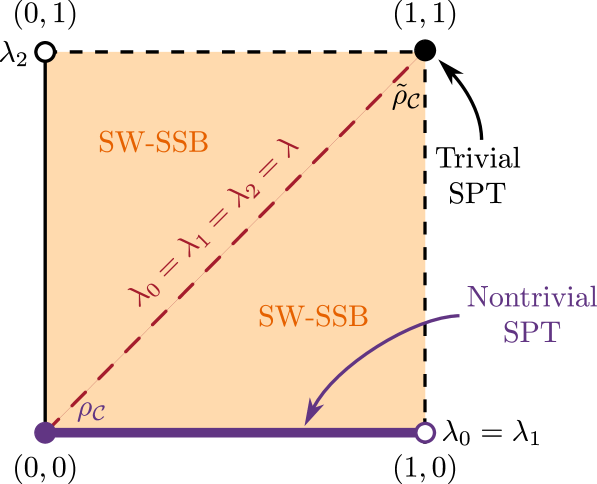
interpolating between the nontrivial SPT Lindbladian [see Section˜III.1] and the trivial-SPT Lindbladian [see Eq.˜29]. We study the steady state of the interpolating Lindbladian using DMRG and calculate various steady state properties, namely the steady-state degeneracy, string order parameters and two other correlators that diagnose strong-to-weak spontaneous symmetry breaking. If there were only one phase transition between the trivial and non-trivial SPT phases, we would expect this transition to take place at the self-dual point . However, as we will show, the instability to SW-SSB leads to a different situation.
IV.1 Mixed-state SPT order
To examine the nontrivial mixed-state SPT order, we calculate the Rényi-1 and Rényi-2 strong-string order parameters, [Eq.˜17] and [Eq.˜21], as well as the Rényi-2 weak-string order parameter, [Eq.˜22], for the steady state of . Recall that, under conjugation by the CZ circuit, and the string operators map as and . We refer to as the nontrivial string order parameters and as the trivial string order parameters.
Upon conjugation by , . Thus the steady states of and are related by conjugation with , or . Hence, calculating the nontrivial string order parameters in the steady states of for all allows us to readily obtain the trivial string order parameters.
For , the steady state in the sector is , which is a nontrivial SPT state having and for any . On the other hand, for , the steady state in the same symmetry sector is [see Eq.˜28], and its nontrivial string order parameters are and its trivial string order parameters are . Recall that a single string order parameter does not determine if the state is in the nontrivial SPT phase or the trivial phase, rather it is the pattern of the string order parameters that determines the phase [55, 37].
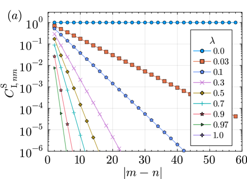
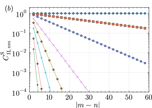
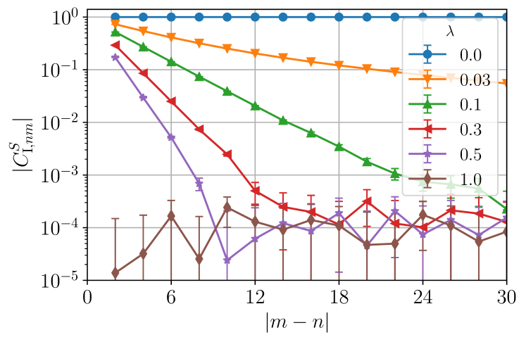
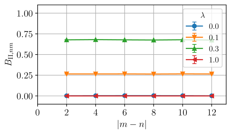
If the nontrivial mixed-state SPT order is stable at , then we expect that after adding a small perturbation , the nontrivial string order parameters will continue to remain nonzero while the trivial string order parameters will continue to remain zero in the limit of long string lengths. In Figs.˜2a and 2b, we show the nontrivial string order parameters evaluated in the steady state in the sector for a system of qubits for various values of . In Figs.˜2a and 2b, we plot the two strong nontrivial string order parameters and for and , which are chosen to minimize the boundary effects. We find that, for all other than and , the strong-string order parameters and both decay exponentially in the string length [see Figs.˜2a and 2b]. For , the trivial strong-string order parameters and also decay to zero exponentially, which can be inferred from the conjugation.
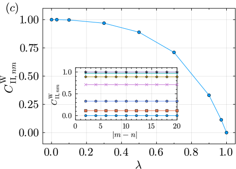
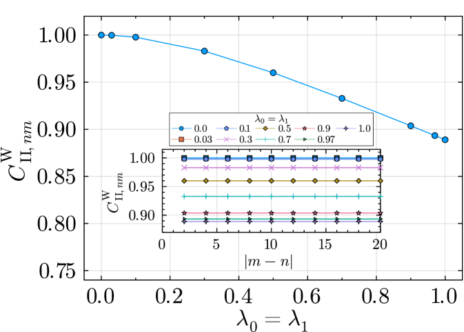
On the other hand, we find that the nontrivial and trivial weak-string order parameters and are independent of the string length and depend only on as shown in the inset of Fig.˜2c. The result is calculated with and varying , and we also plot as a function of in Fig.˜2c. We see that remains nonzero for all . To summarize, the pattern of string order parameters is and for . This matches with the patterns of zeros neither for the nontrivial SPT order nor for the trivial SPT order (see Table 3). This is the first indication that the steady state at any cannot be classified according to the mixed-state SPT state classification, suggesting that the state is neither a nontrivial nor a trivial mixed-state SPT state.
Examining the steady-state degeneracy using DMRG, we find that there is an eight-fold degeneracy for all , where each symmetry sector hosts one steady state. In the Hamiltonian case, the ground state degeneracy is robust to small symmetric perturbations. However, in the case of steady states of Lindbladians, we find that adding a symmetric perturbation with a single jump operator , which acts only on the rightmost qubit, reduces the degeneracy to four. Adding another jump operator further reduces the steady state degeneracy from four to two. From Section˜III.1, we know that a steady state degeneracy of two is guaranteed by the strong symmetry , and indeed, the remaining two steady states reside in the symmetry sectors and , respectively.
IV.2 Strong-to-weak SSB
We have seen that the strong-string order parameters all decay exponentially to zero for any , while the weak-string order parameter is nonzero for . This suggests that the steady state (or ) is not short-range entangled. Furthermore, the trivial strong-string order parameter can also be interpreted as a “disorder” order parameter for the strong symmetry , whose exponential decay with indicates the strong symmetry is spontaneously broken.
In the following, we present evidence for the strong to weak spontaneous symmetry breaking (SSB) of [27, 38, 39] when . We use the following connected correlators to probe strong-to-weak SSB (SW-SSB). For and even, the connected correlators are
| (36) |
| (37) |
| (38) |
where for a density matrix normalized as , is defined in Eq. (20), and the first (second) factor of the tensor product acts on the ket (bra) Hilbert space. For convenience, we provide a summary of these correlators and the string order parameters introduced in Section˜II.5 in Table˜2. Their values in the various phases studied in this work are given in Table˜3.
To see how these correlators probe strong-to-weak SSB, recall that the strong symmetry is in fact two symmetries with the symmetry generator operating on the bra or the ket side independently. In the vectorized perspective (namely, doubled Hilbert space), it is generated by and . The possible symmetry breaking patterns are (broken down to the trivial group) or , where (namely, broken down to a weak symmetry).
We therefore see that the above correlators have the following physical meaning. Since the superoperator is charged under (namely, anti-commutes with) and , we see that is used to detect and the corresponding long-range correlation in . Similarly, anti-commutes with and , so is used to detect and the corresponding long-range correlation in , namely, a long-range correlation quadratic in . On the other hand, anti-commutes with (and ) but commutes with , so is used to detect (but cannot detect if is further broken) and the corresponding long-range correlation in . These patterns of zeros are summarized in Table 3. We note that, in Ref. [38], a fidelity correlator has been proposed as another more robust diagnostic for the strong-to-weak SSB.
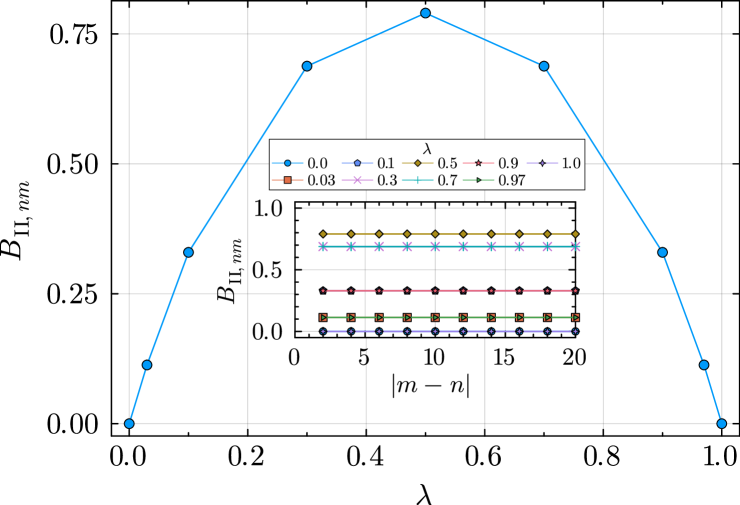
We calculated the correlators , , and of the steady state in the symmetry sector for a system size for various perturbation strengths , fixing and varying . We find that (not shown in the figures), while is a nonzero constant, independent of for all . In Fig.˜3, we plot as a function of . is symmetric about as expected since the operator is invariant under conjugation while maps to . and imply that the weak symmetry on the even sites (which is a subgroup of the strong symmetry on even sites ) is not broken. On the other hand, for implies that the strong symmetry on even sites is broken. Taken these two facts together, we conclude that the perturbation leads to a strong-to-weak SSB on the even sites.
We also study a more general parametrization of the Lindbladians given by
| (39) |
where is composed of the jump operators [see Section˜III.1], and is composed of the jump operators [see Eq.˜29]. Note that . We calculate the steady state of for in the symmetry sector, obtaining the six string order parameters and the three connected correlators that probe SW-SSB in the steady states. This gives us the phase diagram shown in Fig.˜4. We find that the steady state of is in the nontrivial SPT phase for all . We discuss this in more detail in the next section (Section˜IV.3).
In addition to the perturbation, we have also considered a Hamiltonian perturbation with the Hamiltonian proportional to and Lindbladian perturbations with jump operators , , and . In all of these cases, we find that both and decay exponentially to zero, is a nonzero constant independent of , , , and approaches a nonzero constant as is increased. We show these plots in Appendix˜E (Figs.˜11 and 12). This suggests that SW-SSB of the strong symmetry on the even sites is a generic instability of the steady-state mixed-state SPT under our consideration.
We remark that, because of this strong-to-weak SSB, the steady state in the eigenvalue sector of is not an injective matrix-product state. Thus the procedure to extract the projective representation described in Ref. [55] is not applicable.
| Symbol | Defined In | Diagnoses |
| Eqs.˜36 and 37 | SSB | |
| Eq.˜38 | SSB | |
| Eqs.˜17 and 21 | Mixed-state SPT | |
| Eq.˜22 | Mixed-state SPT |
| Phase | |||||||||
| trivial SPT | 0 | 0 | 0 | 0 | 0 | 0 | |||
| SPT | 0 | 0 | 0 | 0 | 0 | 0 | |||
| SSB | 0 | 0 | 0 | 0 | 0 | 0 | |||
| SSB | 0 | 0 | 0 | 0 |
IV.3 Stability against weak-string-order defects
We have seen that adding results in the destruction of the nontrivial SPT order. The instability of the SPT order as a steady state might be expected for the following reason. Recall that, in the dual picture, we can understand the establishment of the strong-string order by the reaction-diffusion process. That is, it would take time to annihilate the strong-string order defects (namely, the local configurations of for even ). Therefore, we expect that, if there is a term in the Lindbladian effectively introducing the strong-string order defects at a constant rate, then the strong-string order in the steady-state will be destroyed. Indeed, we see that the jump operator [defined in Eq.˜29] effectively introduces the strong-string order defects. We note that a recent work [18] proposed to alleviate the above instability by heralding the strong-string defects. However, the unexpected and surprising result of our work is that the destruction of the nontrivial SPT order leads to strong-to-weak symmetry breaking, instead of going to a trivial mixed-state SPT phase.
On the other hand, we ask if the steady-state mixed-state SPT order can be stable against weak-string-order defects. To answer this question, we examine the Lindbladian in Eq. (39) with the parameters on the purple line of Fig.˜4. This can be parameterized as for , corresponding to the perturbations consisting of jump operators on even and on odd , with an equal perturbation strength . For , the steady state is given in Eq.˜3. The jump operators with and with introduce domain wall defects on the odd sites, so we expect that the strong-string order parameters and will remain unity in the perturbed steady states, and the weak-string order parameter will change. As shown in Fig.˜5, remains a nonzero constant for all values of , where the calculation is done for a system of qubits with the steady state of in the symmetry sector. We fix and vary , finding that is independent of for all .
For , we also calculate the nontrivial strong-string order parameters and , finding that they are one for all and for all string lengths as expected. The trivial strong-string correlators and decay exponentially to zero while for all and . This pattern of string order parameters matches with the nontrivial mixed-state SPT as summarized in Table 3. We also find that , indicating that there is no SSB. Thus we find that the mixed-state SPT is stable to perturbations which introduce only weak-string defects.
We comment that with is a pathological point, since the steady-state degeneracy is exponential is . We left such pathological cases as undefined, labeled with open circles in the phase diagram Fig.˜4.
IV.4 Exactly solvable perturbations
As discussed in Section˜III.3, the dynamics generated by the unperturbed Lindbladian in the CZ dual picture [c.f. Eq.˜29] can be decomposed into population dynamics (namely, the diagonal part of the density matrix in the eigenbasis) on the even sites, the effect of which can be mapped to a non-Hermitian free fermion Hamiltonian, as well as dephasing on all the odd sites. This motivates the possibility of considering the perturbations which are exactly solvable via such a free fermion mapping, potentially furthering our understanding of the instability of the steady-state mixed-state SPT toward the SW-SSB.
As we now show, the free fermion mapping also works for a large class of dissipative perturbations to , which can be solved exactly and analytically under periodic boundary conditions. Here, we discuss the manifestation of the SW-SSB, making use of the free fermion analytical solution of the perturbed Lindbladian in those cases. More specifically, we show that, for all perturbing dissipators that can be mapped to a free fermion model via the prescription described in Section˜III.3, the steady state either stays invariant under the perturbation or leads to a SW-SSB.
Before discussing the mapping of perturbative dissipators to free fermion models, we first note that there exist a large group of dissipators that preserve the strong symmetry and do not affect the steady state of . More concretely, from the steady state in Eq. (28), we see that any perturbative dissipator whose jump operator only involves a product of on the even sites would not change the steady state. We can write such perturbed Lindbladian explicitly as , with the jump operators given by
| (40) |
where are parameters characterizing the perturbation that take values or . The jump operator in Eq. (29) provides an example, although there are many more. Furthermore, it is also straightforward to show that, if the jump operator of the perturbation can be written as for any operator , then the actions of and within the population sector (with respect to the eigenbasis) are fully equivalent. We thus focus on jump operators that explicitly involve other Pauli operators.
We now consider possible dissipative perturbations that can be mapped to a free fermion non-Hermitian Hamiltonian under the correspondence in Section˜III.3. In this case, it is straightforward to see that the jump operator can involve at most two spin operators acting on nearest neighbors. One can thus use this constraint along with the symmetry requirement to show that any jump operator that could be mapped to a free fermion Hamiltonian [after performing the Jordan-Wigner transformation in the space spanned by ] should take the following form:
| (41) |
which ensures that corresponds to a quadratic fermion Hamiltonian in the space. Moreover, we require the remaining term of the dissipator to also map to a free fermion Hamiltonian, which means that cannot involve a nontrivial contribution from . We thus prove that any perturbation dissipator that can be mapped to free fermion dynamics should have a jump operator of following form
| (42) |
where or are arbitrary complex coefficients.
As shown in Appendix˜G, the effect of perturbation generated by Eq. (IV.4) on the steady state can always be rewritten as a rescaling of the unperturbed Lindbladian as well as a simpler perturbation . Note that, for perturbations with the specific jump operators , the dual CZ circuit does not change the form of the jump operator, so that we have
| (43) |
where the unperturbed Lindbladian without the dual CZ circuit is given by Eq. (III.1). As such, it suffices to only consider the perturbation and its effect on the steady-state mixed-state SPT order. Intriguingly, as far as the strong-symmetry string order correlators are concerned, the effect of this perturbation (in the original frame without the CZ circuit) is equivalent to adding a perturbation with the jump operator replaced by [see Eq. (25)].
When the aforementioned perturbation preserves translational invariance, i.e. when , we can solve the free fermion non-Hermitian Hamiltonian analytically. The perturbed Lindbladian can be written as
| (44) |
In this case, we can explicitly compute the Rényi-2 strong-string order parameter , as well as the connected correlator in the perturbed state as
| (45) | ||||
| (46) |
We thus see that any free-fermion-type perturbation of the form given in Eq. (IV.4) will lead to an exponentially decaying strong-string order parameter, as well as a finite connected correlator, signaling a strong-to-weak SSB in the perturbed Lindbladian steady state. We conjecture that strong-to-weak SSB is a generic feature of Lindbladian steady states under weak local perturbations (that have a nontrivial impact on the steady state).
We would like to point out that the exactly solvable mapping only applies to certain types of perturbations. For a more general type of perturbations, we refer to Appendix H, where we discuss generic perturbation theory which can capture the physics at small perturbation strengths.
V Clifford circuit realization
So far, we have discussed the steady states of a dynamical open system modeled by a Lindbladian. While there are numerous methods to simulate Lindbladian dynamics on a quantum computer or a quantum simulator [62, 63, 64], here we propose to replicate the essential physics via a local quantum channel instead of trying to simulate the Lindbladian. Furthermore, we construct a quantum channel that can be realized using Clifford gates, Pauli measurements and feedback, allowing us to simulate the quantum dynamics efficiently on a classical computer. It is straightforward to add operations such that the dynamics is no longer efficiently simulable on a classical computer. We note that all Clifford simulations performed in this work were done using the Python package stim [65].
Recall that the parent Lindbladian consists of the jump operators that stabilize the domain-wall configurations (), decohere them (), and make their probabilities uniform (). These actions can be realized by the quantum channel that we now describe.
To stabilize the domain-wall configuration, we use the following measurements and feedback. If is even, we measure ; if the measurement outcome is , we apply the unitary . This can be written as a quantum channel with the following Kraus representation:
| (47) |
where , , and .
The action of and can be mimicked by the following action. If is odd, we measure and then apply the unitary regardless of the measurement outcome, resulting in the quantum channel with a Kraus representation
| (48) |
where for . Note that this channel can also be realized by the following action without a measurement, where we apply the unitary or with an equal probability when .
With the above building blocks, we consider the following channel:
| (49) |
and we consider the steady states of (i.e. applied times) when the number of steps . Note that has the desired symmetry. The channel can be realized by the following procedure. For each step, pick a site from with an equal probability and implement the aforementioned protocol corresponding to depending on being even or odd. corresponds to repeating the above procedure times, which is also the unit of the time step we use.
V.1 Mixing time
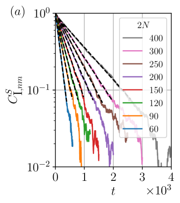
The first quantity we examine is the mixing time of the (unperturbed) quantum channel . As one can easily verify, is a steady state of in the sector, whose strong-string order parameter satisfies . The mixing time is the time that it takes for the channel to take any initial state to the steady state . We instead use the following measure as a proxy for the mixing time. We start with a initial pure state in which . The repeated application of the channel will make grow from to . For a given threshold that is close to , we define the (proxy) mixing time to be the time (number of steps) that it takes for to grow from 0 to .
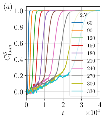
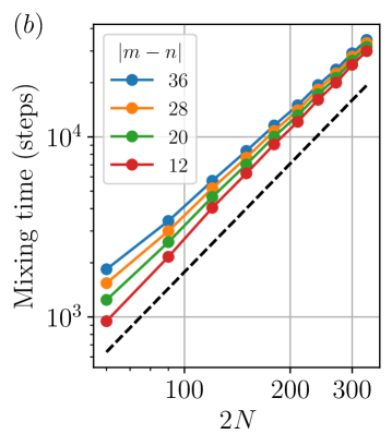
Picking , in Fig.˜6a, we plot as a function of time for system sizes ranging from to and for the end points of the string being at and , so . In Fig.˜6b, we plot the mixing time as a function of system size for various string lengths. We fix and vary to obtain strings of different lengths. For each system size and string length, we average over samples and consider open boundary conditions. We find that the mixing time is approximately asymptotically, which can be understood by thinking of the distance between the defects effectively undergoing a random walk in 1d. Namely, each local channel element has a probability to pick a defect and move it to the right along the chain. For a pair of defects, the distance between them shrinks or grows depending on which defect is picked to move to the right. To approach the steady state , the defects need to pair up and annihilate, where the defects can be separated by a distance of order at late times. Because the standard deviation of the distance of a random walk scales as the square root of time, we expect it to take time to annihilate all defects on average. The mixing time indeed is one of the features of the parent Lindbladian we discussed in Section˜III.3, despite the fact that the Lindbladian and the quantum channel with open boundary conditions are gapped.
V.2 Steady state of perturbed quantum channels
Recall that we studied the steady-state properties of the interpolated Lindbladian for , where is the parent Lindbladian of the trivial SPT state obtained via the conjugation. Here we also consider a similar interpolation achieved by the following channel:
| (50) |
where is the quantum channel of conjugated by . Since and commutes with , we can infer the actions of in and the implementation protocol accordingly. More specifically, the quantum channel corresponds applying or with a probability and , respectively, at each step. If we need to apply , then we just need to follow the procedure outlined for but replacing all by and vice versa. We again are interested in the steady state of when , which can again be efficiently simulated on a classical computer using Clifford simulation.
We examine various correlators of the steady state of the perturbed channel to determine its phase. First, we examine its mixed-state SPT order via the string order parameters. We plot in Fig.˜7 for a system of qubits with open boundary conditions for and various , where the data is obtained by averaging over samples for each string length and each . Here each sample is calculated by averaging the value of in the stabilizer state for time steps after the steady state has been reached. We find that the string correlator decays exponentially with the string length for , indicating that the steady state does not possess nontrivial mixed-state SPT order. This is again similar to the interpolated Lindbladian we studied in Section˜IV.
As discussed previously, we expect that the destruction of the mixed-state SPT order comes from the strong symmetry being spontaneously broken. While not shown in the figures, we confirm this by calculating the correlator, finding that it is exactly zero for all .
To see if the strong symmetry is broken down to the weak symmetry, we need to calculate the correlator. To this end, we need to calculate the purity for the denominator and for the numerator. Since the Clifford simulation generates by sampling a stabilizer state with probability , we can calculate the purity as by averaging over realizations of two-copies of . Likewise, quantities like can be calculated by averaging over realizations of two copies of . The quantities and can be calculated efficiently if is a stabilizer state and , are Pauli operators. This is shown in Appendix˜I, and we outline the algorithm in Algorithm˜1.
However, notice that, for the decohered cluster state , its purity is . This indicates that, in order to obtain a fixed multiplicative accuracy for the purity, one needs the number of samples growing exponentially in . We expect this would also generally be the case for quantities like and for steady states at nonzero . Therefore, we only compute for small sizes .
Fig.˜8 shows a plot of the correlator for a closed chain of 14 qubits. For each and value of in the plot, we average over between and samples. We find that is nonzero for . While not shown in the figures, we also calculate and find that exactly. This indicates that the steady state for indeed has SW-SSB.
V.3 Decay time
We have seen in Section˜V.1 that the time scale for a trivial state to reach the nontrivial mixed-state SPT state scales as in system size. It is therefore interesting to examine the time scale for to reach the SW-SSB steady state under the perturbed quantum channel, and we characterize this “decay time” via the string order parameter . As shown in Fig.˜9a, starts at one in and decays exponentially with time . The exponential-decay form allows us to extract the decay time scale by a linear fit of . In Fig.˜9b, we plot this decay time for a string of length and as a function of system size. Intriguingly, we numerically observe that the decay time scales almost linearly in . It would be interesting to find a simple explanation for this behavior.

V.4 Trajectory dynamics
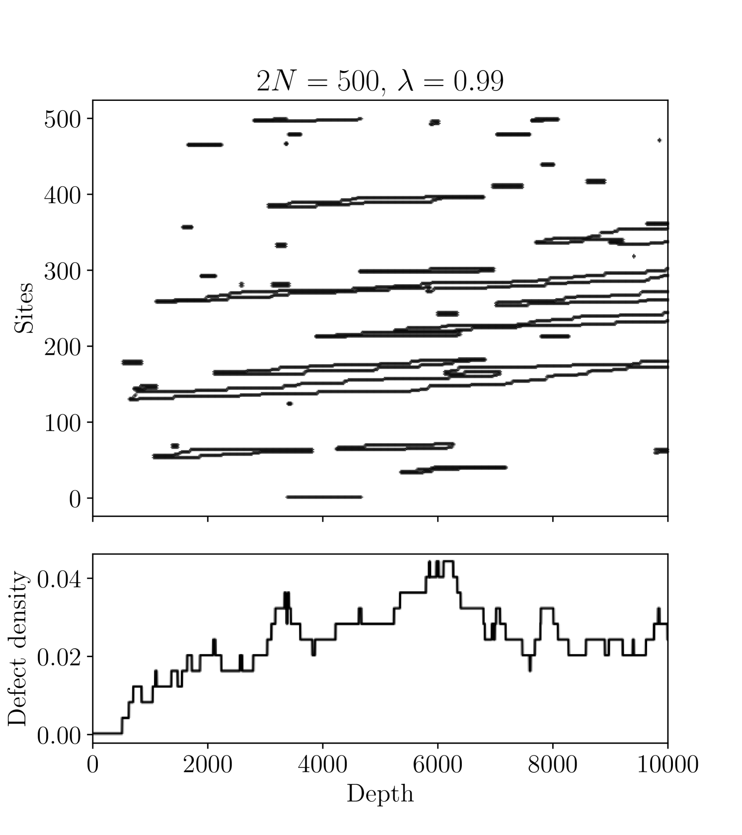
The density matrix at each time step of the channel can be understood as an average over various trajectories, corresponding to different probabilistic outcomes up to that point in the channel’s history. Each of these trajectories exhibits the reaction-diffusion dynamics discussed in Section˜III.3. In order to understand the trajectories of the perturbed channel , we plot the dynamics of defects on even sites. Specifically, we simulate , and at each time step we compute the expectation value of for each even site . When the expectation value is (denoting in black in Fig. 10), we say that site has a defect. The dynamics are such that defects are created and destroyed in pairs. We also plot the defect density—the number of defects divided by —as a function of depth.
As we see in the upper panel of Fig.˜10, defects are created in pairs and propagate probabilistically in a single direction, namely toward the higher numbered sites. Two defects can annihilate if they meet one another, otherwise they continue to propagate. These dynamics result in a nonzero average density of defects at long times, as can be seen in the lower panel of Fig.˜10. The instability of the mixed-state SPT order can be understood as this average density of defects remaining finite for arbitrarily small values of , which results in the destruction of the string order.
VI Discussion
Focusing on the decohered cluster state, we examined some of its characteristics as a mixed-state SPT order, including the bulk-edge correspondence, nontrivial string order, and the corresponding edge states via the matrix-product density operators representation. We then constructed a parent Lindbladian that hosts the decohered cluster state as one of several steady states. Through DMRG and mappings to exactly solvable reaction-diffusion dynamics, we found that the steady-state mixed-state SPT order is unstable to arbitrary small symmetric perturbations, a stark difference from the pure state case. The instability is characterized by the onset of strong-to-weak spontaneous symmetry breaking, which has no counterpart in pure state physics. Based on the dual perspective provided by conjugation, we were able to interpret the destruction of SPT order as a consequence of the proliferation of strong-string-order defects. On the other hand, we found that SPT order is robust against perturbations that generate only weak-string-order defects. We further designed a quantum channel that reproduces the key features of the interpolated Lindbladian we studied. This channel can be efficiently simulated using only Clifford gates, Pauli measurements, and feedback. Using this method to measure observables, we found qualitative agreement with aforementioned results measured in the Lindbladian framework via DMRG. In addition, the quantum channel simulation confirms our expectation of the mixing time scaling while also giving us an intriguing decay time result.
Using the decohered cluster state as a test case, we established the instability of the steady-state mixed-state SPT phase in 1d and of its associated steady-state degeneracy. In particular, the instability comes about due to proliferation of point-like defects-pairs in 1d. These point-like defects must propagate a distance extensive in the system size to meet another defect and annihilate with it. With a restriction to local Lindbladians, or without the global information of the defect locations, the best one can do to annihilate such defects is to make them wander randomly. As pointed out in a recent work [18], one way to alleviate this is by making the defect heralded. We expect that the instability due to such point-like defect proliferation is generic for mixed-state SPT order in 1d.
On the other hand, in 2d, the defects can be line-like rather than point-like. In this case, defect loops can annihilate by contracting to a point rather than fusing with one another, the time-scale for which is no longer extensive in system size. We therefore expect that higher dimensional generalizations of the decohered cluster state—and perhaps steady-state SPT order and the corresponding steady-state degeneracy more generally—may be more stable to local symmetric perturbations.
Another direction that warrants further study is the generalization of the physics we discussed to bosonic systems. For example, the spontaneous strong symmetry breaking down to nothing has been generalized to bosonic open quantum systems, leading to a degenerate steady-state manifold [13]. While we do not expect that the SW-SSB would lead to additional degeneracy other than the ones guaranteed by the strong symmetry, it is still worth investigating if such a phenomenon can be realized in a bosonic system, or even by Gaussian states, which can be readily realized by linear optics.
Our work provides a concrete example that helps pave the way for classifying steady-state phases via their parent Lindbladians [14] instead of the density matrices themselves. One may have thought that adding local symmetric perturbations to the parent Lindbladian cannot lead to any instability. However, we have provided a wide class of examples where this is not the case. It therefore remains an open question of how to construct all potential symmetric perturbations under which the steady-state phases are guaranteed to be stable. Another natural extension of our work is to investigate steady-state phases of other types, including the cases of mixed-state phases of intrinsic topological orders or with symmetry enriched intrinsic topological orders [31, 32, 33].
Acknowledgements.
We thank Meng Cheng, Tyler Ellison, Zhi Li, Ruochen Ma, Connor Mooney, Alex Turzillo, and Yizhi You for valuable discussions and feedback. C.-J.L. acknowledges support from the National Science Foundation (QLCI grant OMA-2120757). J.D.W. acknowledges support from the United States Department of Energy, Office of Science, Office of Advanced Scientific Computing Research, Accelerated Research in Quantum Computing program, and also NSF QLCI grant OMA-2120757. Y.-Q.W. is supported by a JQI postdoctoral fellowship at the University of Maryland. Y.-X.W. acknowledges support from a QuICS Hartree Postdoctoral Fellowship. A.V.G., C.F., J.T.I., J.S., and B.W. were supported in part by the DoE ASCR Accelerated Research in Quantum Computing program (awards No. DE-SC0020312 and No. DE-SC0025341), AFOSR MURI, DARPA SAVaNT ADVENT, NSF QLCI (award No. OMA-2120757), the DoE ASCR Quantum Testbed Pathfinder program (awards No. DE-SC0019040 and No. DE-SC0024220), and the NSF STAQ program. Support is also acknowledged from the U.S. Department of Energy, Office of Science, National Quantum Information Science Research Centers, Quantum Systems Accelerator. C.F. also acknowledges support from NSF DMR-2345644 and from the NSF QLCI grant OMA-2120757 through the Institute for Robust Quantum Simulation (RQS). The authors acknowledge the University of Maryland supercomputing resources (http://hpcc.umd.edu) used in this work.References
- Ma et al. [2019] R. Ma, B. Saxberg, C. Owens, N. Leung, Y. Lu, J. Simon, and D. I. Schuster, A dissipatively stabilized mott insulator of photons, Nature 566, 51 (2019).
- Gertler et al. [2021] J. M. Gertler, B. Baker, J. Li, S. Shirol, J. Koch, and C. Wang, Protecting a bosonic qubit with autonomous quantum error correction, Nature 590, 243 (2021).
- Harrington et al. [2022] P. M. Harrington, E. Mueller, and K. Murch, Engineered Dissipation for Quantum Information Science, Nat. Rev. Phys. 4, 660 (2022).
- Brown et al. [2022] T. Brown, E. Doucet, D. Risté, G. Ribeill, K. Cicak, J. Aumentado, R. Simmonds, L. Govia, A. Kamal, and L. Ranzani, Trade off-free entanglement stabilization in a superconducting qutrit-qubit system, Nat. Commun. 13, 3994 (2022).
- Cole et al. [2022] D. C. Cole, S. D. Erickson, G. Zarantonello, K. P. Horn, P.-Y. Hou, J. J. Wu, D. H. Slichter, F. Reiter, C. P. Koch, and D. Leibfried, Resource-efficient dissipative entanglement of two trapped-ion qubits, Phys. Rev. Lett. 128, 080502 (2022).
- Malinowski et al. [2022] M. Malinowski, C. Zhang, V. Negnevitsky, I. Rojkov, F. Reiter, T.-L. Nguyen, M. Stadler, D. Kienzler, K. K. Mehta, and J. P. Home, Generation of a maximally entangled state using collective optical pumping, Phys. Rev. Lett. 128, 080503 (2022).
- van Mourik et al. [2024] M. W. van Mourik, E. Zapusek, P. Hrmo, L. Gerster, R. Blatt, T. Monz, P. Schindler, and F. Reiter, Experimental realization of nonunitary multiqubit operations, Phys. Rev. Lett. 132, 040602 (2024).
- Coser and Pérez-García [2019] A. Coser and D. Pérez-García, Classification of phases for mixed states via fast dissipative evolution, Quantum 3, 174 (2019).
- Lidar et al. [1998] D. A. Lidar, I. L. Chuang, and K. B. Whaley, Decoherence-free subspaces for quantum computation, Phys. Rev. Lett. 81, 2594 (1998).
- Lidar and Birgitta Whaley [2003] D. A. Lidar and K. Birgitta Whaley, Decoherence-free subspaces and subsystems, in Irreversible Quantum Dynamics, edited by F. Benatti and R. Floreanini (Springer Berlin Heidelberg, Berlin, Heidelberg, 2003) pp. 83–120.
- Mark S. Byrd and Lidar [2004] L.-A. W. Mark S. Byrd and D. A. Lidar, Overview of quantum error prevention and leakage elimination, J. Mod. Opt. 51, 2449 (2004).
- Albert [2018] V. V. Albert, Lindbladians with multiple steady states: theory and applications (2018), arXiv:1802.00010 .
- Lieu et al. [2020] S. Lieu, R. Belyansky, J. T. Young, R. Lundgren, V. V. Albert, and A. V. Gorshkov, Symmetry breaking and error correction in open quantum systems, Phys. Rev. Lett. 125, 240405 (2020).
- Rakovszky et al. [2024] T. Rakovszky, S. Gopalakrishnan, and C. von Keyserlingk, Defining stable phases of open quantum systems (2024), arXiv:2308.15495 .
- Ma and Wang [2023] R. Ma and C. Wang, Average symmetry-protected topological phases, Phys. Rev. X 13, 031016 (2023).
- Ma et al. [2023] R. Ma, J.-H. Zhang, Z. Bi, M. Cheng, and C. Wang, Topological phases with average symmetries: The decohered, the disordered, and the intrinsic (2023), arXiv:2305.16399 .
- Niu and Qi [2023] Y. Niu and Y. Qi, Strange Correlator for 1D Fermionic Symmetry-Protected Topological Phases (2023), arXiv:2312.01310 .
- Chirame et al. [2024] S. Chirame, F. J. Burnell, S. Gopalakrishnan, and A. Prem, Stable Symmetry-Protected Topological Phases in Systems with Heralded Noise (2024), arXiv:2404.16962 .
- Guo et al. [2024] Y. Guo, J.-H. Zhang, H.-R. Zhang, S. Yang, and Z. Bi, Locally Purified Density Operators for Symmetry-Protected Topological Phases in Mixed States (2024), arXiv:2403.16978 .
- Paszko et al. [2024] D. Paszko, D. C. Rose, M. H. Szymańska, and A. Pal, Edge modes and symmetry-protected topological states in open quantum systems, PRX Quantum 5, 030304 (2024).
- Veríssimo et al. [2023] L. M. Veríssimo, M. L. Lyra, and R. Orus, Dissipative Symmetry-Protected Topological Order, Phys. Rev. B 107, L241104 (2023).
- Zhang et al. [2023] J.-H. Zhang, K. Ding, S. Yang, and Z. Bi, Fractonic higher-order topological phases in open quantum systems, Phys. Rev. B 108, 155123 (2023).
- Xue et al. [2024] H. Xue, J. Y. Lee, and Y. Bao, Tensor network formulation of symmetry protected topological phases in mixed states (2024), arXiv:2403.17069 .
- Zhang et al. [2024a] Z. Zhang, U. Agrawal, and S. Vijay, Quantum Communication and Mixed-State Order in Decohered Symmetry-Protected Topological States (2024a), arXiv:2405.05965 .
- Zhang et al. [2024b] J.-H. Zhang, Y. Qi, and Z. Bi, Strange correlation function for average symmetry-protected topological phases (2024b), arXiv:2210.17485 .
- Lee et al. [2024] J. Y. Lee, Y.-Z. You, and C. Xu, Symmetry protected topological phases under decoherence (2024), arXiv:2210.16323 .
- Ma and Turzillo [2024] R. Ma and A. Turzillo, Symmetry protected topological phases of mixed states in the doubled space (2024), arXiv:2403.13280 .
- Hsin et al. [2023] P.-S. Hsin, Z.-X. Luo, and H.-Y. Sun, Anomalies of Average Symmetries: Entanglement and Open Quantum Systems (2023), arXiv:2312.09074 .
- Lessa et al. [2024a] L. A. Lessa, M. Cheng, and C. Wang, Mixed-state quantum anomaly and multipartite entanglement (2024a), arXiv:2401.17357 .
- Wang and Li [2024] Z. Wang and L. Li, Anomaly in open quantum systems and its implications on mixed-state quantum phases (2024), arXiv:2403.14533 .
- Bao et al. [2023] Y. Bao, R. Fan, A. Vishwanath, and E. Altman, Mixed-state topological order and the errorfield double formulation of decoherence-induced transitions (2023), arxiv:2301.05687 .
- Lee et al. [2023] J. Y. Lee, C.-M. Jian, and C. Xu, Quantum criticality under decoherence or weak measurement, PRX Quantum 4, 030317 (2023).
- Ellison and Cheng [2024] T. Ellison and M. Cheng, Towards a classification of mixed-state topological orders in two dimensions (2024), arXiv:2405.02390 .
- Garre-Rubio et al. [2023] J. Garre-Rubio, L. Lootens, and A. Molnár, Classifying phases protected by matrix product operator symmetries using matrix product states, Quantum 7, 927 (2023).
- Buča and Prosen [2012] B. Buča and T. Prosen, A note on symmetry reductions of the lindblad equation: transport in constrained open spin chains, New J. Phys. 14, 073007 (2012).
- Albert and Jiang [2014] V. V. Albert and L. Jiang, Symmetries and conserved quantities in Lindblad master equations, Phys. Rev. A 89, 022118 (2014).
- de Groot et al. [2022] C. de Groot, A. Turzillo, and N. Schuch, Symmetry protected topological order in open quantum systems, Quantum 6, 856 (2022).
- Lessa et al. [2024b] L. A. Lessa, R. Ma, J.-H. Zhang, Z. Bi, M. Cheng, and C. Wang, Strong-to-Weak Spontaneous Symmetry Breaking in Mixed Quantum States (2024b), arXiv:2405.03639 .
- Sala et al. [2024] P. Sala, S. Gopalakrishnan, M. Oshikawa, and Y. You, Spontaneous Strong Symmetry Breaking in Open Systems: Purification Perspective (2024), arXiv:2405.02402 .
- Hastings and Wen [2005] M. B. Hastings and X.-G. Wen, Quasiadiabatic continuation of quantum states: The stability of topological ground-state degeneracy and emergent gauge invariance, Phys. Rev. B 72, 045141 (2005).
- Chen et al. [2013] X. Chen, Z.-C. Gu, Z.-X. Liu, and X.-G. Wen, Symmetry protected topological orders and the group cohomology of their symmetry group, Phys. Rev. B 87, 155114 (2013).
- Briegel and Raussendorf [2001] H. J. Briegel and R. Raussendorf, Persistent entanglement in arrays of interacting particles, Phys. Rev. Lett. 86, 910 (2001).
- Son et al. [2012] W. Son, L. Amico, and V. Vedral, Topological order in 1d cluster state protected by symmetry, Quantum Information Processing 11, 1961 (2012).
- Lushnikov [1986] A. Lushnikov, Binary reaction in one dimension, Zh. Eksp. Teor. Fiz 91, 1376 (1986).
- Pachos and Plenio [2004] J. K. Pachos and M. B. Plenio, Three-spin interactions in optical lattices and criticality in Cluster Hamiltonians, Phys. Rev. Lett. 93, 056402 (2004).
- Doherty and Bartlett [2009] A. C. Doherty and S. D. Bartlett, Identifying phases of quantum many-body systems that are universal for quantum computation, Phys. Rev. Lett. 103, 020506 (2009).
- Gottesman [1998] D. Gottesman, The heisenberg representation of quantum computers (1998), arXiv:quant-ph/9807006 .
- Chen et al. [2014] X. Chen, Y.-M. Lu, and A. Vishwanath, Symmetry-protected topological phases from decorated domain walls, Nat. Commun. 5, 3507 (2014).
- Cubitt et al. [2015] T. S. Cubitt, A. Lucia, S. Michalakis, and D. Perez-Garcia, Stability of local quantum dissipative systems, Commun. Math. Phys. 337, 1275 (2015).
- Onorati et al. [2023] E. Onorati, C. Rouzé, D. S. França, and J. D. Watson, Provably efficient learning of phases of matter via dissipative evolutions (2023), arXiv:2311.07506 .
- Lieb and Robinson [1972] E. H. Lieb and D. W. Robinson, The finite group velocity of quantum spin systems, Commun. Math. Phys. 28, 251 (1972).
- Poulin [2010] D. Poulin, Lieb-robinson bound and locality for general Markovian quantum dynamics, Phys. Rev. Lett. 104, 190401 (2010).
- den Nijs and Rommelse [1989] M. den Nijs and K. Rommelse, Preroughening transitions in crystal surfaces and valence-bond phases in quantum spin chains, Phys. Rev. B 40, 4709 (1989).
- Kennedy and Tasaki [1992] T. Kennedy and H. Tasaki, Hidden symmetry breaking in Haldane-gap antiferromagnets, Phys. Rev. B 45, 304 (1992).
- Pollmann and Turner [2012] F. Pollmann and A. M. Turner, Detection of symmetry-protected topological phases in one dimension, Phys. Rev. B 86, 125441 (2012).
- Else et al. [2013] D. V. Else, S. D. Bartlett, and A. C. Doherty, Hidden symmetry-breaking picture of symmetry-protected topological order, Phys. Rev. B 88, 085114 (2013).
- Bahri and Vishwanath [2014] Y. Bahri and A. Vishwanath, Detecting Majorana fermions in quasi-one-dimensional topological phases using nonlocal order parameters, Phys. Rev. B 89, 155135 (2014).
- Lindblad [1976] G. Lindblad, On the generators of quantum dynamical semigroups, Commun. Math. Phys. 48, 119 (1976).
- Gorini et al. [1976] V. Gorini, A. Kossakowski, and E. C. G. Sudarshan, Completely positive dynamical semigroups of N-level systems, J. Math. Phys. 17, 821 (1976).
- Lin and Zou [2021] C.-J. Lin and L. Zou, Reaction-diffusion dynamics in a Fibonacci chain: Interplay between classical and quantum behavior, Phys. Rev. B 103, 174305 (2021).
- Fishman et al. [2022] M. Fishman, S. R. White, and E. M. Stoudenmire, The ITensor Software Library for Tensor Network Calculations, SciPost Phys. Codebases , 4 (2022).
- Kliesch et al. [2011] M. Kliesch, T. Barthel, C. Gogolin, M. Kastoryano, and J. Eisert, Dissipative quantum Church-Turing theorem, Phys. Rev. Lett. 107, 120501 (2011).
- An et al. [2023] D. An, J.-P. Liu, and L. Lin, Linear combination of Hamiltonian simulation for nonunitary dynamics with optimal state preparation cost, Phys. Rev. Lett. 131, 150603 (2023).
- Purkayastha et al. [2021] A. Purkayastha, G. Guarnieri, S. Campbell, J. Prior, and J. Goold, Periodically refreshed baths to simulate open quantum many-body dynamics, Phys. Rev. B 104, 045417 (2021).
- Gidney [2021] C. Gidney, Stim: a fast stabilizer circuit simulator, Quantum 5, 497 (2021).
- Chen et al. [2023] C.-F. Chen, M. J. Kastoryano, and A. Gilyén, An efficient and exact noncommutative quantum Gibbs sampler (2023), arXiv:2311.09207 .
- Rouzé et al. [2024] C. Rouzé, D. S. França, and Á. M. Alhambra, Efficient thermalization and universal quantum computing with quantum Gibbs samplers (2024), arXiv:2403.12691 .
- Bergamaschi et al. [2024] T. Bergamaschi, C.-F. Chen, and Y. Liu, Quantum computational advantage with constant-temperature Gibbs sampling (2024), arXiv:2404.14639 .
- Rajakumar and Watson [2024] J. Rajakumar and J. D. Watson, Gibbs sampling gives quantum advantage at constant temperatures with O(1)-local Hamiltonians (2024), arXiv:2408.01516 .
- Sang and Hsieh [2024] S. Sang and T. H. Hsieh, Stability of mixed-state quantum phases via finite Markov length (2024), arXiv:2404.07251 .
Appendix A A Lindbladian definition of mixed state phases
In this appendix, we show that is also a nontrivial SPT state according to the “fast-driving Lindbladian” definitions of Refs. [8, 37], complementing the finite-depth quantum channel result obtained in Refs. [15, 16]. In Coser and Pérez-García [8], two mixed states are defined to be in the same phase if there are local Lindbladian evolutions which can rapidly bring the two states close to each other. While Ref. [8] essentially implies that all the mixed states are in the “trivial” phase in 1d if the symmetry of the Lindbladian evolution is weak, de Groot et al. [37] demonstrate that one can have nontrivial SPT states by requiring that the Lindbladian evolution respects the strong symmetry of the system. Below, we review the definition of two states being in the same phase according to Refs. [8, 37].
Definition 1 (Fast Driving).
Given two states and , we say that can be driven fast to if there exists a local time-independent Lindbladian such that
for some time , where and the trace distance . We denote it as
Definition 2 (Lindbladian Phase of Matter).
We say that and are in the same phase if there exist local symmetric time-independent Lindbladians and such that and .
The intuition behind this definition is that, if one state can be reached by a -time evolution from another state, then the long-range correlations in the two states must be similar. Furthermore, this rapid mixing condition implies stability of local observables to local perturbations in the Lindbladian terms when away from the boundaries of the phase [49, 50]. Moreover, it is a natural and physically motivated generalization of the Hamiltonian definition of phases to open systems. Indeed, Coser and Pérez-García demonstrate that this Lindbladian definition encompasses that standard gapped-Hamiltonian phase of matter. Furthermore, it can be shown that it encompasses high-temperature thermal phases using the Lindbladian of Chen et al. [66, 67], and this even applies to families of states that are classically intractable to prepare [68, 69].
Compared to previous works using this definition [8, 50], we have removed the auxiliary system as it is not required for this work. However, anything that satisfies this more restricted definition of phase must also satisfy the definition of phase in Ref. [8]. We also note recent work in Ref. [70] where it has been shown that this Lindbladian definition implies that two states are in the same phase if one can smoothly move between fixed points without the “correlation length” for the mutual information diverging. Here by “correlation length”, we mean the length scale over which the mutual information decays exponentially.
Here we demonstrate that the decohered cluster state cannot be in the trivial phase by the Coser and Pérez-García as per Defs. 1 and 2 if the Lindbladian respects a symmetry. To prove this, we first realize that any state evolving under a local Lindbladian has an associated speed limit on the speed of information propagation, known as the Lieb-Robinson velocity [52].
More formally, consider a local observable , supported only on a region . Let be an area of distance around , and let be the Lindbladian restricted to only terms that are in . Assuming the Lindbladian is a sum of local terms and the strength of each local term is bounded as , we have
| (51) |
for constants from Ref. [49, Lemma 5.5] or Ref. [52]. In the case that the Lindbladian acts trivially on parts of , we replace on the right-hand side with the size of the region which acts nontrivially on i.e. is now the set of sites where . Using this, we are able to prove the following theorem.
Theorem 1.
Proof.
Note that, since the Lindbladian commutes with the strong symmetry , the string part of the order parameter remains invariant under the Lindbladian evolution because the bulk of the string is made of symmetry operators . The Lindbladian is therefore only acting nontrivially on the end parts of . Denote and to be the regions within a distance of the end points , respectively. Applying Eq.˜51 we get
| (53) | ||||
We note that, although acts over an area, due to the symmetry condition, it only acts nontrivially on an area, hence .
We now consider the expectation value of the string order parameter on any state in the trivial phase. By the Coser & Pérez-García definition of phase, we can write any state in the trivial phase as for an appropriate Lindbladian, where is a reference product state in the trivial phase and . Now consider
| (54) | ||||
where we have applied Eq.˜53 to reach the second line.
Since , we can choose a localized Lindbladian which contains the Lieb-Robinson light-cone by choosing for . Since we have assumed , we see that for some constant . Thus we can write
To reach the second line, we have split the product state into a part supported on and its complement, and we have used that and have disjoint supports, hence . Since the Lindbladian preserves the symmetry operator, we see that the endpoint operators have the same charge as in the non-time-evolved case, hence we can write
and thus
The immediate consequence is that, for any state in the trivial phase, it cannot be the case that as increases.
∎
Appendix B Fast destruction of strong-string order
In this appendix, we show the fast destruction of the strong-string order for odd and as defined in the main text in Eq.˜18. The destruction of the strong-string order can be achieved by a trace channel where . It is easy to check that indeed satisfies the symmetry and is of depth one.
Assume is a nontrivial SPT state and denote . We would like to calculate . It is easy to check that , so we have where is the trivial string operator defined in Eq.˜23 and the paragraph succeeding it. We therefore see that , indicating that the strong-string order is being destroyed via a depth-one symmetric quantum channel.
This result can also be generalized to the Lindbladian case. Consider the following trace Lindbladian: . Note that
| (55) |
where denotes all the possible sets of , is the number of sites in the set , and is the trace channel on the set . Note that . We have
| (56) |
Therefore, for a time , . This implies that a nontrivial state can be driven fast to a trivial state when . We therefore conclude that the mixed-state SPT order is hard to build but easy to destroy.
Appendix C String order of
In this appendix, we will show that has nontrivial string order under the same string order parameters as . First recall that we may express in the vectorized picture as
| (57) |
Next, observe that
| (58) |
where we have defined to be the distance between and within the even sublattice. Notice that each term in the summand depends only on due to translational invariance. Defining the tensor diagram appearing in Eq.˜58 to be , we have
| (59) | ||||
where we have replaced the sum over and with a sum over and a multiplicity factor of which accounts for the different possible endpoints separated by sites.
Now, consider the numerator of the two-copy expectation value of the strong-string :
| (60) | ||||
where we have defined to be if and otherwise and used the fact that . This sum is nearly the same as that appearing in Eq.˜59, but some terms now appear with a minus sign. For a particular choice of , there will be terms for which lies between and and therefore for which . We can therefore write
| (61) | ||||
Combining Eq.˜59 and Eq.˜61, we find
| (62) | ||||
We can perform a similar calculation of the two-copy expectation value of the weak-string order parameter. Consider
| (63) | ||||
so that
| (64) |
We can also calculate the expectation value of the 1-copy string order parameters. Again, using vectorized tensor network notation for the density matrix, we have
| (65) | ||||
where we have once again defined to be if and otherwise and used the fact that .
Finally, we have
| (66) | ||||
where we have again used the fact that . We see that the density matrix exhibits non-trivial string order under the one- and two-copy string order parameters used to characterize the decohered cluster state.
Appendix D Some details of DMRG
In this appendix, we provide some details behind how we obtain the steady states of the Lindbladians via DMRG. First, we vectorize the density matrices by the following mapping:
| (67) |
Note that we choose the ordering of the qubits in the doubled Hilbert space as opposed to ordering. This is done to preserve the locality of the vectorized Lindbladian . Using this mapping, we construct the vectorized Lindbladian and provide it as an input to the dmrg function in ITensors with ishermitian = false argument. Setting this argument gives the eigenstate of the vectorized Lindbladian that has the smallest real part of the eigenvalue. Since, for the steady state, we have , and the eigenvalues of are nonnegative, the state obtained after DMRG has converged is one of the steady states. To obtain the steady state in the sector, we project the output of DMRG into that sector by calculating , where
| (68) | ||||
To make sure that the output of DMRG, say , is an eigenstate with a good enough numerical precision, we also compute the variance of the vectorized Lindbladian of the state as
| (69) |
where . If is an eigenstate of , then the variance should be 0. Thus calculating the variance serves as a good check to ensure that we have an eigenstate of , which typically has a value of about in our calculations.
Appendix E Other perturbations
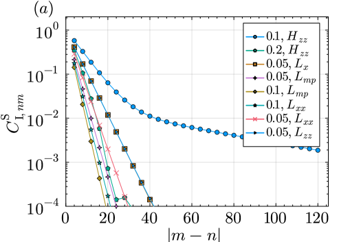
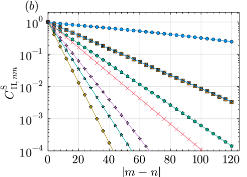
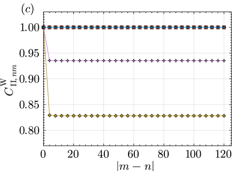
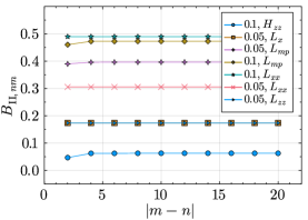
In this appendix, we present the results for other symmetric perturbations that we have examined, which include Hamiltonian perturbations as well as Lindbladian perturbation. Specifically, we consider the Hamiltonian perturbation and the Lindbladian perturbation of the form , where the jump operators can take one of the following (with ):
| (70) |
and the sum is over all the allowed values of . These perturbations are added separately with a small perturbation strength to the parent Lindbladian . It is interesting to note that in the CZ dual picture, [see Eq. (25) in the main text], while stays invariant as , so that those two perturbations generate identical strong string order correlators; this agrees well with the numerical DMRG calculations, see Fig. 11 and the following discussions.
We calculate the steady state of the perturbed Lindbladian in the symmetry sector using DMRG. We then calculate the six string order parameters defined in Section˜IV.1 and the three connected correlators defined in Section˜IV.2 to probe SW-SSB. We find that all the correlators indicate strong-to-weak SSB on even sites, with some of the correlators plotted in Figs.˜11 and 12. For these plots, the system size is qubits, and the left end of the correlator for is kept fixed at while the right end is varied in . For , we fix and vary ; for , we fix and vary . We find that the connected correlators and are identically zero. Also, unlike the Lindbladian considered in Section˜IV.2, the correlator is independent of for a generic perturbation as shown in Fig.˜12. In conclusion, our numerical results suggest that the steady-state mixed-state SPT state is generically unstable to SW-SSB (unless the perturbation only introduces weak symmetry defects like the one in Section˜IV.3).
Appendix F Finite-size scaling of string order parameters
The results of Sections˜IV.1 and IV.2 show that the steady-state mixed-state SPT order is unstable for any small perturbation , leading to strong-to-weak SSB. In this appendix, we perform finite-size scaling of the Rényi-1 strong-string order parameter which further shows the scaling relation between the perturbation strength and system size . First, we show our scaling collapse result for the following Lindbladian:
| (71) |
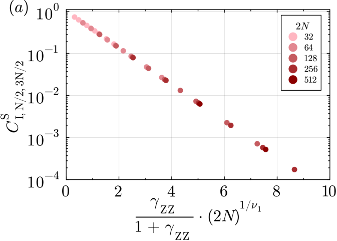
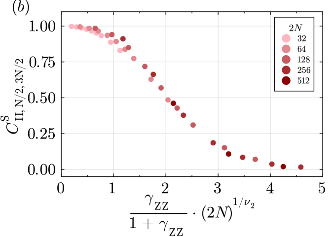
For a range of system sizes that vary from to and perturbation strengths , we calculate the strong-string order parameters and , where and so the string length is . We use the following scaling ansatz:
| (72) |
for some function . We find good data collapse for as shown in Fig.˜13a, which also shows that decays exponentially with . Note that here we simply try and find good collapse rather than fitting the data to a function and finding the value of for which the fit is the best. For the Rényi-2 correlator, , we fit a sixth degree polynomial and find the value of that minimizes the residual error of the fit. Doing so gives us the optimal value of . and we find that the data collapses for this value of as shown in Fig.˜13b.
We perform a similar analysis for the interpolated Lindbladian in Eq.˜35, and we employ the scaling ansatz
| (73) |
Again we find an excellent collapse for as shown in Fig.˜13a without any fitting. For , we again minimize the residual error in fitting a sixth degree polynomial to the data to determine the optimal value of at which the collapse happens. We find the optimal value of to be , and the data collapses reasonably well as shown in Fig.˜13b.
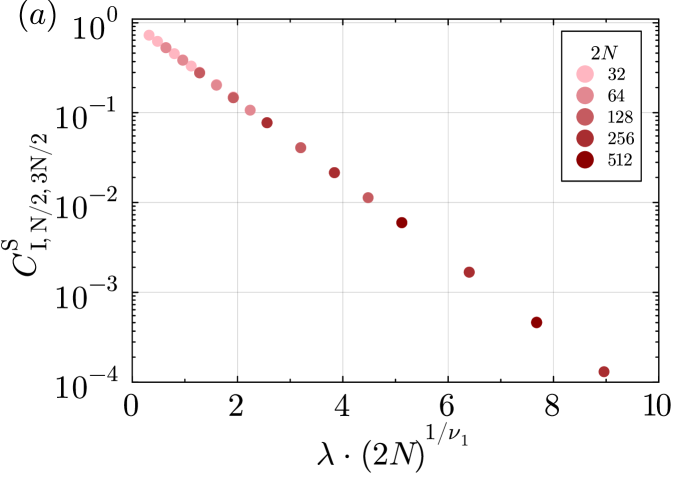
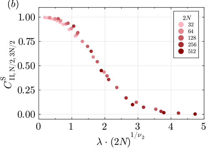
Appendix G Free fermion solution to the Lindbladian dynamics with ZZ perturbation
As mentioned in the main text, dynamics generated by the parent Lindbladian as well as a certain class of perturbations can be exactly solved by the mapping to a non-Hermitian free fermion Hamiltonian. In this appendix, we discuss in more detail the solution and its implications for mixing times and various order parameters.
We consider the following Lindbladian acting on all the even sites:
| (74) | ||||
| (75) |
Our goal is to solve for the spectrum of . To achieve this, we first note that, since the Lindbladian has a weak symmetry generated by for all (which is a subgroup of the strong symmetry ), the dynamics generated by the Lindbladian is decoupled between the basis populations (i.e., the diagonal part) versus the coherences (i.e., the off-diagonal part) of the density matrix. Therefore, we can exactly map the action of the Lindbladian to a non-Hermitian Hamiltonian acting on the vectors spanned by the corresponding basis states to the population or the coherence sectors. For example, focusing on the population sector that also hosts the even-parity steady state, we consider the following mapping (introducing the basis states , and we use to distinguish the mapped state from the pure state wavefunction of the original system):
| (76) |
in which case the Lindbladian equation of motion can be mapped to a linear equation of motion of the state vector :
| (77) |
Note that the equation above takes a form similar to the standard Schrödinger equation, but with a non-Hermitian dynamical generator (which in this case is given by the non-Hermitian operator ). The generator of non-Hermitian dynamics is given by
| (78) |
which can be written in terms of the spin raising and lowering operators as
| (79) | ||||
| (80) | ||||
| (81) |
It is interesting to note that the non-Hermitian Hamiltonian describes a one-dimensional spin chain that only involves quadratic terms acting on nearest-neighbor sites, which can be mapped to a free fermion non-Hermitian Hamiltonian via the standard Jordan-Wigner (JW) transformation. More concretely, introducing fermion operators via the JW prescription as
| (82) |
we obtain
| (83) | ||||
| (84) | ||||
| (85) |
The spectrum of the free fermion non-Hermitian Hamiltonian can be generally computed by solving for its right eigenmodes , which are the solutions to the following eigenvalue equation:
| (86) |
Here, we make use of the fact that the eigenvalues of come in pairs , as is invariant under the anti-unitary transformation consisting of the combination of Hermitian conjugation and reflection of the one-dimensional chain . Without loss of generality, we require .
If the lattice is translationally invariant, we can take and without loss of generality. The eigenvalue equation Eq. (86) can then be solved analytically by Fourier transforming the real space free fermion to momentum space. After some algebra, we obtain
| (87) |
with the corresponding right eigenmode operators given by
| (88) |
The steady state as defined by can thus be written as
| (89) |
where the coefficients can be expressed as
| (90) |
For a chain with even number of sites, we have , and the above sum over can be evaluated explicitly as
| (91) | ||||
| (92) |
Note that, in the unperturbed case (), the steady state is . We also note that the steady state solution given by Eq. (92) agrees with the results in Ref. [44], which considered the specific case with . However, Ref. [44] did not consider the case with bidirectional hoppings in the unperturbed Lindbladian, and to the best of our knowledge, previous works did not compute the correlators in this non-Hermitian free fermion problem, which we show below.
As shown above, the steady state structure in fact does not depend on the directionality of hopping (as parametrized by ). Transforming the fermion operators back into the spin ones, we have
| (93) |
We can further compute all two-body correlators making use of the solution in Eq. (89), as
| (94) |
G.1 Mixing time
We note that the full Lindbladian spectrum in the population sector can be generated by Eq. (87). The Lindblad equation of motion for the coherences in the basis can be mapped to a similar non-Hermitian Hamiltonian Eq. (78) by a modified mapping, which also corresponds to a non-Hermitian free fermion Hamiltonian, and we expect the coherences to decay faster compared to the minimal decay rate in the population sector. We can thus directly compute the spectral (Lindbladian) gap , i.e. the smallest real part of the Lindbladian eigenvalues, via the smallest real part of the free fermion non-Hermitian Hamiltonian eigenvalues . From Eq. (87), we can calculate the Lindbladian gap as
| (95) |
In the large-system-size limit, the spectral gap of the unperturbed Lindbladian with thus scales as
| (96) |
We note that this also sets a lower bound on the mixing time scaling of the open boundary Lindbladian in the thermodynamic limit, as in the open-boundary-conditions case, relaxation dynamics in the bulk is agnostic to the boundary conditions.
G.2 Connected correlators & strong-string order parameter
It is worth noting that, when the Lindbladian steady state only involves populations in the basis, then the correlators , as defined in the main text must be trivially zero.
Further, we can directly use the wavefunction in the mapping Eq. (76) to compute the Rényi-2 correlators and the Rényi-2 strong string order parameters, as by definition, the Rényi-2 expectation value of an operator can be written in terms of as
| (97) |
and expectation averages of the mapped wavefunction can be computed using the free fermion state by Wick’s theorem. As an example, we consider
| (98) |
and one can straightforwardly show that for all even and any steady state with only populations in the basis, so that we have . From Eqs. (76) and (93), we thus have
| (99) |
which can be rewritten in terms of the fermion operators as
| (100) |
We can also compute the two-copy strong symmetry order parameter, defined in Eq. (21), as
| (101) |
Appendix H Overview of perturbation theory
As mentioned in Section˜IV.4 of the main text, the exactly solvable mapping only applies to certain kinds of perturbations. In this appendix, we discuss a general perturbation theory which can capture the physics of sufficiently small perturbations that cannot be exactly solved by the procedure of Section˜IV.4. In particular, we will start from the CZ dual of the parent Lindbladian and add a perturbation which is a linear combination of the dissipators formed by the jump operators shown in Eq.˜29 with a small perturbation strength. Referring to Section˜III.2 of the main text, we define as the density matrix of the unperturbed state with qubits, where is the density matrix defined in Eq.˜28:
| (102) |
For simplicity, we only consider up to the first order in perturbation theory. Note that each jump operator of Eq.˜29, when acting on defined in Eq.˜102, will either leave unchanged or give the following matrices:
| (103) |
where , and
| (104) |
The above perturbation process can be mapped to an intuitive “particle hopping” picture, where the particles are defect sites with . The () has zero (two) defect sites with , and can be mapped to a classical state with zero (two) particles. More specifically, we use the notation to denote a classical basis state [c.f. Eq.˜76]. We map the original problem with qubits to a chain of hard-core bosons with sites, such that the density matrix in the original problem of qubits is mapped to the classical states in the hard-core boson problem as follows:
| (105) |
Here () describes the classical state where no (one) boson sits on site of the hard-core boson chain. The density matrix defined in Eq.˜102 is mapped to the classical state with no bosons on the chain, which we denote as . The density matrix in Eq.˜103 is mapped to a classical state that describes the state with two bosons on sites on the chain of hard-core bosons.
After mapping to the particle hopping picture, the perturbed dynamics can be captured by the Markovian transition matrix . The unperturbed transition matrix corresponds to and consists of processes in which one of the two bosons in a classical state hops rightwards. For example, it can take to . The perturbation to the transition matrix, , corresponds to . The perturbation leads to two new effects in addition to the effects produced by . The first effect is that it can generate a pair of bosons at sites out of [i.e. it can take the classical state from to the state ]. The second effect is that it can lead to the simultaneous hopping of two bosons sitting on sites to sites , where and . In other words, it takes one classical state to another classical state .
We further denote the steady state of the unperturbed transition matrix, i.e, the right eigenvector of with eigenvalue zero, as , so that . Taking the first-order perturbed right eigenvector as , we have
| (106) |
To leading order in , we have
| (107) |
where is the pseudoinverse of .
The steady state of the transition matrix of the hard-core boson hopping problem can then be described by
| (108) |
where is the coefficient of the vacuum state , is the coefficient of the state , is the coefficient of the state , etc… These coefficients are normalized to one according to
| (109) |
After solving for the steady states of the perturbed particle hopping problem, we can determine the steady state of the original problem defined on qubits via
| (110) |
Here captures the steady state in the presence of perturbation on top of . It is easy to check that under the normalization condition we considered.
One can then compute the string order parameters in the perturbed steady state up to first order in the perturbation. Consider the strong-string operator , shown in Eq.˜18, which acts on the original model of qubits as an example:
| (111) |
with and odd, , and even. Since we are working in the CZ dual picture, we consider the CZ dual of the string operator, . is defined as
| (112) |
where is given in Eq.˜27. It is easy to check that . Similarly, we have for or , and otherwise. Given the above, we can compute the string order parameters defined in Eq. (17) as
| (113) |
where sums over all the cases that satisfy or . Note that we have used the normalization condition for and given in Eq. (109). Thus, given a perturbation , we can determine the perturbation to the transition matrix, . We can then calculate the coefficients and efficiently numerically. Plugging these coefficients into Eq.˜113 gives us the string correlator up to first order in perturbation theory.
Appendix I Stabilizer-state calculations
In this appendix, we briefly outline the algorithm to calculate quantities like and for stabilizer states and and Pauli operators and .
Assume the stabilizer states and are stabilized by the stabilizers generated by and , respectively. We then have . We therefore see that , which is the probability of measuring on with all outcomes. We therefore also see that, if is a Pauli operator, is also a stabilizer state. So can be calculated accordingly.
We now describe how to compute . Consider , where is still a stabilizer state, and . We must therefore compute for stabilizer states and a Pauli operator . Note that . Again, assume the stabilizers of are generated by , then is the probability of measuring with outcomes all for but outcomes for . However, note that, for a stabilizer state , the probability difference between the measurement outcome and is exactly .
This yields the following procedure (see Algorithm˜1). The idea is to force the state into a eigenstate of each stabilizer generator of , while keeping track of the probabilities of being in such an eigenstate. Then, we can simply compute the expectation value of in . To calculate , we can simply take .
Note that in Algorithm˜1, there are three possible branches for : (the if branch), (the else if branch), and (the else branch). The else branch is not included in the pseudocode for Algorithm˜1 because it is redundant. The else condition () would proceed as and postselect onto the eigenstate of . But if , then is already in the eigenstate of , thus making the else condition redundant.