Intelligent Reflecting Surface Assisted Multi-Cluster AirComp via Dynamic Beamforming
Abstract
This paper studies an multi-cluster over-the-air computation (AirComp) system, where an intelligent reflecting surface (IRS) assists the signal transmission from devices to an access point (AP). The clusters are activated to compute heterogeneous functions in a time-division manner. Specifically, two types of IRS beamforming (BF) schemes are proposed to reveal the performance-cost tradeoff. One is the cluster-adaptive BF scheme, where each BF pattern is dedicated to one cluster, and the other is the dynamic BF scheme, which is applied to any number of IRS BF patterns. By deeply exploiting their inherent properties, both generic and low-complexity algorithms are proposed in which the IRS BF patterns, time and power resource allocation are jointly optimized. Numerical results show that IRS can significantly enhance the function computation performance, and demonstrate that the dynamic IRS BF scheme with half of the total IRS BF patterns can achieve near-optimal performance which can be deemed as a cost-efficient approach for IRS-aided multi-cluster AirComp systems.
Index Terms:
Intelligent reflecting surface (IRS), over-the-air computation (AirComp), dynamic beamforming (BF), computation rate maximization.I Introduction
The sixth generation (6G) network aims to integrate communication, sensing, computing, and intelligence together, thus constructing native multi-functional systems that serve as powerful engines to build an intelligent world [1, 2, 3]. A series of advanced services are progressively conceived and experimented in such multi-functional systems, such as extended reality (XR), edge artificial intelligence (AI), and autonomous driving [4, 5], either of which needs to collect and process enormous data from distributed devices. Conventionally, the raw data collection and process are regarded as separate procedures and designed in isolation.
In practice, these intelligent services demand the functional computation results of the raw data, such as the maximum reading of several temperature monitors, the average of local models, and the minimum distance between cars and barricades. The recently aroused over-the-air computation (AirComp), deemed as a task-oriented multiple-access (MA) strategy, has shown its high efficiency in integrating communication and computation through leveraging the signal superposition characteristic of the wireless channel [6]. The co-channel interference is treated as a catalyst in AirComp for computation, whereas traditional task-agnostic MA techniques consider it to be detrimental. AirComp was conceived [7, 8] and validated [9] to be a promising scalable function computation strategy in a series of works. Specifically, the transceiver design that exhibits a uniform-forcing structure to compensate individual channel fading was proposed in [10], and the multiple-input multiple-output (MIMO) AirComp [7] was exploited for simultaneously multi-modal sensing. However, the harsh wireless propagation environment still significantly weakens the signal strength and thus deteriorates the computation performance.
Intelligent reflecting surface (IRS), a promising technology for future wireless networks, has shown the potential to overcome this detrimental effect by adapting the phase shifts of low-cost passive elements. Several works have exhibited the effectiveness of IRSs in the single-cluster AirComp system, e.g., the authors in [11, 12] employed an IRS to strengthen channels thus reduce the distortion. If the single-cluster AirComp is intuitively extended to a multi-cluster case like the conventional communication systems [13, 6], the considered configuration times of IRS passive beamforming (BF) is the same as the number of participated clusters, otherwise its BF remains static during a transmission frame, i.e., each cluster is assigned with a dedicated BF pattern or all clusters employ the same pattern. It is observed that the two policies are rigid in that they provide the upper and lower bounds on system performance with no tradeoff. Although harnessing more BF patterns provides more degrees of freedom (DoFs) which can configure a suitable propagation environment for devices, thereby further enhancing the system performance, it also adds extra signaling overhead. Hence, a flexible dynamic IRS BF scheme is desired to balance the system performance and cost. Recently, a novel dynamic IRS beamforming (DIBF) technique has been proposed to offer promising DoF thus enabling more flexible resource allocation in half-duplex and full-duplex wireless powered communication networks (WPCNs) [14, 15], mobile edge computing (MEC) with binary offloading [16], etc. DIBF proactively develops favorable time-selective channels by harnessing the unique character of IRSs that the BF patterns can be tuned multiple times within a given channel coherence time. Additionally, a good balance between performance, associated tuning costs, and signaling overhead can be achieved by flexibly managing the amount of reconfigurations.
In this work, we analyze an IRS-aided AirComp system comprising of multiple clusters by taking the performance-cost tradeoff into account. The previous studies concentrated on the transceiver design in one dedicated time slot (TS) that aim to minimize the function computation error measured by the mean square error (MSE). We study in this paper how to boost the computation capability within a given period in which the IRS can be configured multiple times. Specifically, clusters are activated in a time-division manner to eliminate the inter-cluster interference thereby computing heterogeneous functions, and we present two types of BF schemes to unleash the fundamental performance-cost tradeoff. The cluster-adaptive BF method, where each BF is allocated to one cluster, is first taken into consideration to provide the upper bound for comparison. The performance-cost tradeoff is then explored using the general dynamic IRS BF method, which is be applied to any number of BF patterns. Simulation results verify the theoretical findings and show how IRS improves the performance of multi-cluster AirComp. In particular, it is observed that the proposed DIBF design is sufficient to acquire near-optimal performance with a minimal computation rate decrease (less than ) by halving the number of BF patterns, which sheds light on balancing the performance-cost via limiting the number of BF patterns.
II System Model and Problem Formulation
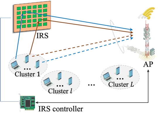
As depicted in Fig. 1, the considered multi-cluster AirComp system composes of a single antenna access point (AP), an IRS equipped with passive elements, and devices. Due to the different computational requirements, the devices are divided into clusters. Each cluster consists of devices and computes a desired type- function named . We denote as the set of devices within -th cluster, where . The AP computes heterogeneous functions via AirComp from each cluster in a time-division manner. Specifically, the AP computes with the raw data from all the devices in cluster . Let denote one dedicated reading of the device in cluster . The target type- function computed at AP is expressed as
| (1) |
where is the pre-processing function at device , and is the post-processing function at the AP. We adopt the digital AirComp to perform function computation, in which the nest lattice coding strategy is harnessed to achieve the integer combinations of transmitted codewords and combat the channel noise meanwhile. Specifically, the reading of each device is first processed by , then the result is quantized and mapped into a vector, and finally, it is encoded into a nested lattice codeword (see [17, 13] for more details). We assume that each symbol of the transmitted signal has been normalized into a mutual independent symbol with zero mean and unit power. Hence, the target recovered data at the AP of cluster when computing a type- function is given by .
The baseband channels from the IRS to AP, from the device to IRS, and from the device to AP are denoted by , and , respectively. In this paper, we assume that all the involved channels are perfectly known by applying the state-of-the-art channel estimation techniques [18]. All devices in each cluster transmit concurrently with the symbol-level synchronization assumed. In a channel coherence interval , the duration required to compute a function is further divided into TSs. In addition, , where is employed in, denotes the time interval for the -th TS. Then, is divided to sub-TSs for the function computation in different clusters. In sub-TS , the recovered signal from cluster to compute is given by
| (2) |
where are the transmitter and the receiver scalars, respectively. Besides, denotes the composite device-AP channel coefficient of device in cluster , where denotes the phase shift matrix of IRS, in which denotes the phase shift on the incident signal of -th element [19], with , and denotes the additional white Gaussian noise.
The landmark work in [17] established the fundamentals of compute-and-forward strategy from the information theory perspective. Accordingly, the subsequent work [13] proposed the computation rate of AirComp, defined as the achieved number of computed function values per channel use (in num/Hz), which can be expressed as
| (3) |
with being the number of the optimal quantization bits for the type- function computation, being the number of involved devices, and . It can be observed from (3) that the computation rate maximization problem can be equivalently transformed into the MSE minimization problem. By adopting the uniform-forcing transceiver proposed in [10], the solution to the MSE minimization problem is
| (4) |
where denotes the maximum allowed transmit power. Similarly, for the case when devices are energy-limited, we have
| (5) |
where is the allocated power of device for current transmission. The corresponding computation rate of cluster under BF pattern is given by
| (6) |
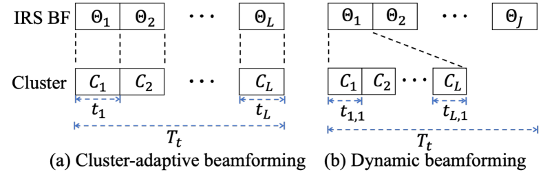
We aim to boost the computation capability within in which IRS can be configured multiple times. As shown in Fig. 2, the two proposed IRS BF schemes depend on how the IRS sets its BF during the time interval, and are specified as follows.
II-A Cluster-adaptive IRS BF
Each cluster is mapped with a unique IRS BF pattern as well as the TSs in the cluster-adaptive BF scheme, which provide the performance upper bound, i.e., arbitrary BF schemes with cannot further improve the performance [14]. Accordingly, the computation rate maximization problem is given by
| (7a) | ||||
| (7b) | ||||
| (7c) | ||||
| (7d) | ||||
| (7e) | ||||
where denotes the weight of cluster . Since the weight , quantization bit , and the number of devices of each cluster do not affect the scheme design, we set that . Note that (P1) is generally a non-convex optimization problem with non-convex norm-one constraint (7e) and the coupled variables in (7a) and (7d).
II-B Dynamic IRS BF
For the proposed general framework that the BF at IRS can be reconfigured times during , the clusters can flexibly choose one or multiple BF patterns for computation. The corresponding problem is formulated as
| (8a) | ||||
| (8b) | ||||
| (8c) | ||||
| (8d) | ||||
| (8e) | ||||
Similar to (P1), we assume that . Note that (P2) is still non-convex since there exist highly-coupled variables in both (8a) and (8d), and constraint (8e) is generally non-convex.
III Proposed Algorithms
III-A Proposed Algorithm for (P1)
(P1) is shown as a maximin problem, which can be converted to a traditional maximization problem by intuitively introducing the auxiliary variables to substitute the inner minimization part. Then, multiple techniques can be adopted, such as alternating optimization. However, it is still inefficient and may suffer from performance loss. In this section, by analyzing the inherent properties of (P1), we propose an efficient algorithm correspondingly.
Proposition 1.
The optimal solution of (P1) satisfies,
| (9) |
Proof: Suppose that achieves the optimal solution to (P1), we have . The maximum allowed transmit power for the devices in cluster becomes . By combing it with (4), Proposition 1 is obtained.
Inspired by Proposition 1, we introduce the auxiliary variables that satisfy and reformulate (P1) as
| (10a) | ||||
| (10b) | ||||
| (10c) | ||||
Note that the objective function is jointly concave with and , thus the difficulty of problem (10) consists of the non-convex constraints (10b) and (7e).
Let and . Exploiting the matrix lifting technique, i.e., define , we have . Besides, we convert the rank-one constraint of to a difference-of-convex form and add it to objective function as
| (11a) | ||||
| (11b) | ||||
| (11c) | ||||
| (11d) | ||||
where is the penalty factor, and denotes the spectral norm of . The factor is harnessed to penalize the violation of the rank-one constraint. Note that when , hence the obtained solution satisfies the rank-one constraint. For any given and any given point in the -th iteration, by linearizing to via the successive convex approximation (SCA) technique,111 is the eigenvector corresponding to the biggest eigenvalue. problem (11) is converted to a convex optimization problem. Hence, by decreasing the value of and updating in each iteration, the convergence of proposed algorithm for (P1) can be finally reached [15].
III-B Proposed Algorithms for (P2)
For (P2), we reveal the following proposition to simplify the original problem and then propose an efficient algorithm.
Proposition 2.
The optimal solution of (P2) satisfies
| (12) |
where denotes the maximum energy of the devices in cluster allocated for IRS BF pattern , which satisfies .
Proof: Suppose that achieves the optimal solution to (P2), we have . The maximum allowed transmit power for the devices in cluster under BF pattern becomes . By combing it with (4), Proposition 2 is obtained.
According to Proposition 2, (P2) can be reformulated as
| (13a) | ||||
| (13b) | ||||
| (13c) | ||||
By introducing the auxiliary variables that satisfy , we have
| (14a) | ||||
| (14b) | ||||
| (14c) | ||||
Introducing slack variables , it yields
| (15a) | ||||
| (15b) | ||||
| (15c) | ||||
Since the objective value can always be increased by raising until the constraint (15b) becomes active, it can be seen that the constraint (15b) is satisfied with equality for the optimal solution to problem (15).
Observing that the objective function of problem (15) is show as a concave function with respect to the variables and , but the constraints (8e), (14b), and (15b) are still non-convex. First, we convert (15b) into
| (16) |
and then apply SCA technique to linearize the right-hand sides of (16) with given points in the -th iteration as
| (17) |
Second, we convert (14b) to
| (18) |
and linearize it as
| (19) |
in which is the given point in iteration . Furthermore, problem (15) is approximated as a convex optimization problem by loosening (8e) to which can be addressed by the standard solvers, the corresponding unit-modulus BF patterns are then obtained by subtracting the phases.
The proposed algorithm for tackling the dynamic IRS BF scheme is shown as solving a series of convex problems. Specifically, problem (15) has five kinds of variables, the last of which has dimension , and the others are . Hence, the corresponding computational complexity is given by via the interior-point method [20], in which stands for the quantity of iterations required to attain convergence. Note that the amount of constraints and optimization variables scale linearly with the number of participated clusters and BF patterns , it can be observed that the related computational complexity is extraordinarily large.
Remark 1.
By analyzing (P2), we can observe that the optimal association between IRS BF patterns and clusters is binary [14], i.e., each cluster only needs to select one BF pattern to compute the function.
Low-complexity algorithm for (P2): Inspired by Remark 1 and the cluster-adaptive BF scheme, we can propose an efficient low-complexity algorithm. We assume that each cluster is assigned with a specific BF as the cluster-adaptive scheme presented in Section III-A.The clusters are then arranged in descending order by their respective computation rates. Each of the first clusters is given with a dedicated BF pattern and the remaining clusters are assumed to employ the same BF pattern . Finally, we jointly optimize the time allocation and . By relaxing the norm-one constraints of IRS BF, the computational complexity of the first phase is given by [20]. The maximum computation complexity of the sorting algorithm is given by . With given IRS BF, we have where . Reformulate the problem as (14), the remaining variables to be optimized is , where the dimensions are given by , respectively. By linearizing the non-convex constraint respect to via SCA technique and relaxing the norm-one constraint, the problem can be converted to a convex one. Hence, the overall computational complexity of this low-complexity algorithm is given by [20].
IV Simulation Results
In this section, we provide numerical results to demonstrate the efficiency of the proposed schemes and the insights for IRS-aided multiple-cluster AirComp system. The AP and the IRS are located at meter (m) and m, respectively. The placement of each device is random within a radius of m that centered at m. The path-loss exponents of the AP-devices channels are set to 3.3, whereas the path-loss exponents for the AP-IRS and IRS-devices channels are set to 2.3. Additionally, the signal attenuation at a reference distance of m is set as dB. Unless otherwise stated, other parameters are set as: , , J, dBm, and s. For comparison, we consider the following schemes: 1) Upper bound: relaxing the rank-one constraint in problem (11), which serves as a performance upper bound; 2) Cluster-adaptive BF: the approach in Section III-A to solve (P1); 3) Dynamic BF: the approach in Section III-B to solve (P2); 4) Low-complexity algorithm: the proposed low-complexity algorithm for (P2).
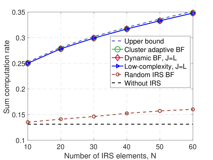
In Fig. 3, we analyze the system performance versus the number of IRS elements . It can be seen that the dynamic IRS BF designs in the case of can perform almost as well as the special case with cluster-adaptive BF and nearly as the upper bound. Additionally, it can be seen that the low-complexity algorithm is capable of achieving the same performance as the joint optimization strategy. This shows the applicability of the proposed DIBF design. In comparison to the cases that BFs are randomly given and without IRS, it is observed that the proposed algorithms can greatly enhance computation rate, with the performance gap widening as the number of IRS elements rises. Besides, the computation rate of IRS-assisted AirComp with optimized IRS phase monotonically increases with respect to the number of IRS elements since more elements can reflect more captured signal energy.
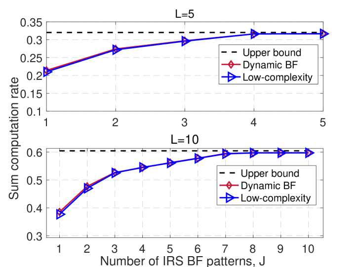
As shown in Fig. 4, we depict the computation rate versus the number of available BF patterns . It can be seen that the low-complexity algorithm for DIBF can achieve similar performance as the previously proposed joint optimization algorithm, making it more desirable in practice. In addition, one can see that the dynamic IRS BF scheme’s performance improvement progressively reaches saturation as rises. Employing a total of ( BF patterns is virtually able to attain the maximum performance for (), and adding further only results in a marginal performance enhancement. It is further noted that the proposed DIBF design can achieve nearly optimal computation rate with a negligible performance loss (less than ) with only half the number of the maximum BF patterns, demonstrating its potential to meet the performance-cost tradeoff by managing the number of BF patterns.
V Conclusion
In this paper, we studied the IRS-aided multi-cluster AirComp system and proposed two types of IRS BF schemes, which struck a balance between the system performance and cost. By jointly optimizing the time allocation for various clusters, the phase shifts at IRS, and the power allocation at devices, the sum computation rate maximization problems for the two scenarios were addressed. We proposed both general and low-complexity algorithms to tackle the optimization problem with any number of IRS BF patterns, and thus provided considerable flexibility in balancing between the performance gain of DIBF and its consequent system cost. Numerical results demonstrated that IRS can significantly improve the function computation performance, and presented the performance-cost tradeoff for IRS-aided AirComp. In particular, the dynamic IRS BF scheme was validated to be a cost-efficient strategy to achieve close-to-optimal performance with only half number of IRS BF patterns, and the proposed low-complexity algorithm can achieve satisfactory performance compared to the generic design.
References
- [1] X. You et al., “Towards 6G wireless communication networks: Vision, enabling technologies, and new paradigm shifts,” Sci. China Inf. Sci., vol. 64, no. 1, pp. 1–74, Jan. 2021.
- [2] K. B. Letaief, Y. Shi, J. Lu, and J. Lu, “Edge artificial intelligence for 6G: Vision, enabling technologies, and applications,” IEEE J. Sel. Areas Commun., vol. 40, no. 1, pp. 5–36, Jan. 2022.
- [3] X. Li et al., “Integrated sensing, communication, and computation over-the-air: MIMO beamforming design,” IEEE Trans. Wireless Commun., early access, doi: 10.1109/TWC.2022.3233795.
- [4] W. Saad, M. Bennis, and M. Chen, “A vision of 6G wireless systems: Applications, trends, technologies, and open research problems,” IEEE Netw., vol. 34, no. 3, pp. 134–142, May 2020.
- [5] Y. Shi, K. Yang, T. Jiang, J. Zhang, and K. B. Letaief, “Communication-efficient edge AI: Algorithms and systems,” IEEE Commun. Surv. Tutorials, vol. 22, no. 4, pp. 2167–2191, 4th Quat., 2020.
- [6] Z. Wang, Y. Zhao, Y. Zhou, Y. Shi, C. Jiang, and K. B. Letaief, “Over-the-air computation: Foundations, technologies, and applications,” 2022, arXiv: 2210.10524. [Online]. Available: https://arxiv.org/abs/2210.10524
- [7] G. Zhu and K. Huang, “MIMO over-the-air computation for high-mobility multimodal sensing,” IEEE Internet Things J., vol. 6, no. 4, pp. 6089–6103, Aug. 2019.
- [8] Y. Zhao et al., “Performance-oriented design for intelligent reflecting surface assisted federated learning,” IEEE Trans. Commun., early access, doi: 10.1109/TCOMM.2023.3283799.
- [9] H. Guo et al., “Over-the-air aggregation for federated learning: Waveform superposition and prototype validation,” J. Commun. Inf. Networks, vol. 6, no. 4, pp. 429–442, Dec. 2021.
- [10] L. Chen, X. Qin, and G. Wei, “A uniform-forcing transceiver design for over-the-air function computation,” IEEE Wirel. Commun. Lett., vol. 7, no. 6, pp. 942–945, Dec. 2018.
- [11] Z. Wang, J. Qiu, Y. Zhou, Y. Shi, L. Fu, W. Chen, and K. B. Letaief, “Federated learning via intelligent reflecting surface,” IEEE Trans. Wirel. Commun., vol. 21, no. 2, pp. 808–822, Jul. 2022.
- [12] X. Zhai, G. Han, Y. Cai, and L. Hanzo, “Beamforming design based on two-stage stochastic optimization for RIS-assisted over-the-air computation systems,” IEEE Internet Things J., vol. 9, no. 7, pp. 5474–5488, Apr. 2022.
- [13] M. Goldenbaum, H. Boche, and S. Stanczak, “Nomographic functions: Efficient computation in clustered gaussian sensor networks,” IEEE Trans. Wirel. Commun., vol. 14, no. 4, pp. 2093–2105, Apr. 2015.
- [14] Q. Wu, X. Zhou, W. Chen, J. Li, and X. Zhang, “IRS-aided WPCNs: A new optimization framework for dynamic IRS beamforming,” IEEE Trans. Wirel. Commun., vol. 21, no. 7, pp. 4725–4739, Jul. 2022.
- [15] M. Hua and Q. Wu, “Joint dynamic passive beamforming and resource allocation for IRS-aided full-duplex WPCN,” IEEE Trans. Wirel. Commun., vol. 21, no. 7, pp. 4829–4843, Jul. 2022.
- [16] G. Chen, Q. Wu, R. Liu, J. Wu, and C. Fang, “IRS aided MEC systems with binary offloading: A unified framework for dynamic IRS beamforming,” IEEE J. Sel. Areas Commun., vol. 41, no. 2, pp. 349–365, Feb. 2023.
- [17] B. Nazer and M. Gastpar, “Compute-and-forward: Harnessing interference through structured codes,” IEEE Trans. Inf. Theory, vol. 57, no. 10, pp. 6463–6486, Oct. 2011.
- [18] Q. Wu, S. Zhang, B. Zheng, C. You, and R. Zhang, “Intelligent reflecting surface-aided wireless communications: A tutorial,” IEEE Trans. Commun., vol. 69, no. 5, pp. 3313–3351, Jan. 2021.
- [19] Q. Wu and R. Zhang, “Intelligent reflecting surface enhanced wireless network via joint active and passive beamforming,” IEEE Trans. Wirel. Commun., vol. 18, no. 11, pp. 5394–5409, Aug. 2019.
- [20] S. J. Wright, Primal-dual interior-point methods. SIAM, 1997.