Intelligent Reflecting Surfaces and Classical Relays: Coexistence and Co-Design

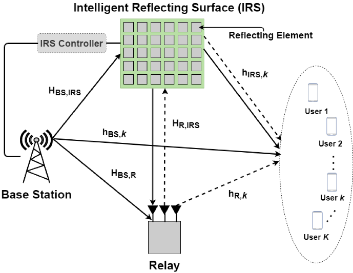
As shown in Fig. 1, we consider a downlink MU-MISO communication system that comprises a BS with $M$ antennas, $K$ single-antenna end users, an IRS with $N$ reflecting elements, and a classical half-duplex DF relay with $L$ antennas. Here, to ensure a sufficient degree of freedom, we assume $K\leq\min\{M,L\}$. The baseband equivalent channels between two communication nodes among the BS, IRS, relay, and user $k$ are denoted by self-explanatory notations ${\mathbf{H}}_{{\rm BS},{\rm R}}\in{\mathbb{C}}^{L\times M}$, ${\mathbf{H}}_{{\rm BS},{\rm IRS}}\in{\mathbb{C}}^{N\times M}$, ${\mathbf{h}}_{{\rm BS},k}\in{\mathbb{C}}^{1\times M}$, ${\mathbf{H}}_{{\rm R},{\rm IRS}}\in{\mathbb{C}}^{N\times L}$, ${\mathbf{h}}_{{\rm R},k}\in{\mathbb{C}}^{1\times L}$, and ${\mathbf{h}}_{{\rm IRS},k}\in{\mathbb{C}}^{1\times N}$. All channels are assumed to be quasi-static and Rayleigh flat-fading. The small-scale fading is modeled by complex Gaussian with zero mean and unit variance and the large-scale fading is modeled by $\kappa{\left({d}/{d_{0}}\right)}^{-\varrho},$ where $d$ is the distance between the two end nodes, $d_{0}$ is the reference distance, $\kappa$ is a large-scale fading constant, and $\varrho$ is the path-loss exponent. The CSI of all channels is assumed perfectly known at the BS, the IRS controller, and the relay. Due to the presence of the relay, there are two phases in one complete transmission of information, for which the first phase and the second phase are assumed to be within the channel coherence interval. Moreover, in this paper, reflecting elements can be adjusted by the IRS controller once in each complete transmission of the information. Next, we elaborate on the two-phase transmission protocol.

In this paper, we aim for maximizing the sum-rate of all the users by jointly optimizing the active beamforming at the BS, the active beamforming at the relay, and the passive beamforming at the IRS. Specifically, the optimization problem is formulated as

where the optimization variables and objective function are given in (8a), $\{\mathbf{g}_{k}\}$ and $\{\mathbf{f}_{k}\}$ are the sets of the BS beamforming and the relay beamforming vectors for all users, respectively. Constraints (8b) and (8c) denote the available transmit power at the BS and the DF relay, respectively. Constraint (8d) is the reflection constraint for an ideal IRS. Constraint (8e) ensures the decoding SINR requirements for all users’ signals at the relay are satisfied. Note that the pre-log factor of $1/2$ due to two-phase transmission is dropped in the achievable rate expression, but is considered in all simulations.

Solving the problem in (8) is a challenging task, as the optimization variables are highly coupled, rendering a nonconvex problem. To tackle the problem, we propose an alternating optimization (AO)-based algorithm to decouple (8) into three subproblems, as detailed in the next section.

Given fixed relay beamforming vectors $\{{\mathbf{f}}_{k}\}$ and IRS beamforming matrix $\mathbf{\Theta}$, the problem in (8) becomes

where $C_{1,k}=1+\gamma_{k}^{\rm II},$ $k=1,\ldots,K$ are considered as constants under the AO-based decomposition. The subproblem (9) is still nonconvex and difficult to solve. In this subsection, we tackle the subproblem in (9) by first transforming the problem of finding $\mathbf{g}_{k}$ into one of finding the rank-one positive semidefinite matrix ${\mathbf{G}}_{k}=\mathbf{g}_{k}{\mathbf{g}}_{k}^{\rm H}$ and then by relaxing the rank-one constraint, which eventually leads to a convex semidefinite programming (SDP) problem. Toward this end, we develop the following four steps 1) introducing slack variables, 2) first-order Taylor approximation, 3) alternating optimization, and 4) semidefinite relaxation, as detailed below.

Given fixed $\{{\mathbf{g}}_{k}\}$ (obtained from the steps in Sec. III-A) and $\mathbf{\Theta}$, the problem of solving the relay beamforming $\{\mathbf{f}_{k}\}$ in (8) becomes

where $C_{2,k}=1+\gamma_{k}^{\rm I},k=1,2,\ldots,K$, are kept as constants. The subproblem for finding the relay beamforming vector $\mathbf{f}_{k}$ in (18) is nonconvex. Following similar steps developed in Sec. III-A, we elaborate on how to convexify (18) below.

Let ${\mathbf{F}}_{k}={\mathbf{f}}_{k}{\mathbf{f}}_{k}^{\rm H}$. Define the slack variables $\{{\mathcal{S}}_{2,k}\}$ and $\{{\mathcal{I}}_{2,k}\}$ that satisfy

where ${\mathbf{h}}^{\prime\prime}_{{\rm R},k}\triangleq{{\mathbf{h}}^{\prime}_{{\rm R},k}}^{\rm H}{\mathbf{h}}^{\prime}_{{\rm R},k}$. With the above slack variables, the subproblem (18) can be equivalently rewritten as

where $u_{2}(\bf z)$ is for notational convenience. Similarly, we apply Taylor approximation on $u_{2}(\bf z)$ and obtain a lower bound $R_{2,k}^{\rm low}$, which has closed-form expression from $\nabla u_{2}({\bf z}^{\rm loc})$. Then, (21) can be converted to

The solution set of (22) is a subset of the solution set of (21), since the lower bound $R_{2,k}^{\rm low}$ is used in the constraint (21b). By relaxing the rank-one constraint in (21c), we can solve the resulting SDP problem with CVX. Finally, as in the case in Sec. III-A, the randomization procedure can be employed to obtain rank-one solutions for $\{{\mathbf{f}}_{k}\}$, $k=1,\ldots,K$.

Given fixed BS beamforming $\{{\mathbf{g}}_{k}\}$ and relay beamforming $\{{\mathbf{f}}_{k}\}$ (respectively obtained from the steps in Sec. III-A and Sec. III-B), the problem of solving the IRS beamforming matrix $\boldsymbol{\Theta}$ (or equivalently its vector form $\boldsymbol{\theta}$) in (8) becomes

We adopt similar steps as in Secs. III-A and III-B to solve (23). To facilitate finding the optimal IRS beamforming matrix $\boldsymbol{\Theta}$, we re-arrange the order of $\boldsymbol{\Theta}$ in (1) and in (5) respectively to ${y}_{k}^{\rm I}={\boldsymbol{\phi}}^{\rm H}{\mathbf{H}}_{{\rm B},{\rm I},k}{\mathbf{x}}+w_{k}^{\rm I}$ and $y_{k}^{\rm II}={\boldsymbol{\phi}}^{\rm H}{\mathbf{H}}_{{\rm R},{\rm I},k}{\mathbf{x}}_{\rm R}+w_{k}^{\rm II},$ where ${\boldsymbol{\phi}}={\begin{bmatrix}{\boldsymbol{\theta}}&1\end{bmatrix}}^{\rm H}$, ${\mathbf{H}}_{{\rm B},{\rm I},k}=\begin{bmatrix}{\rm diag}({\mathbf{h}}_{{\rm IRS},k}){\mathbf{H}}_{{\rm BS},{\rm IRS}}\\ {\mathbf{h}}_{{\rm BS},k}\end{bmatrix}$, and ${\mathbf{H}}_{{\rm R},{\rm I},k}=\begin{bmatrix}{\rm diag}({\mathbf{h}}_{{\rm IRS},k}){\mathbf{H}}_{{\rm R},{\rm IRS}}\\ {\mathbf{h}}_{{\rm R},k}\end{bmatrix}$. With the reordering, the slack variables $\{{\mathcal{S}}_{1,k}\}$, $\{{\mathcal{I}}_{1,k}\}$, $\{{\mathcal{S}}_{2,k}\}$, and $\{{\mathcal{I}}_{2,k}\}$ respectively in (10), (11), (19), and (20) can be rewritten as

where $\mathbf{\Phi}\triangleq{\boldsymbol{\phi}}{\boldsymbol{\phi}}^{\rm H}$. Similarly, we can re-arrange the order of $\boldsymbol{\Theta}$ in (3), by which the slack variables $\{{\mathcal{S}}_{{\rm R},k}\}$ and $\{{\mathcal{I}}_{{\rm R},k}\}$ in (12) and (13) can be rewritten in terms of $\mathbf{\Phi}$.

With the above slack variables, we have the following equivalent problem

where $u_{3}({\bf z})$ and $v_{3}({\bf z}_{\rm R})$ respectively defined in (28b) and (28c) are for notational convenience. Next, using the first-order Taylor approximation, as in the previous sections, lower bounds of $u_{3}({\bf z})$ and $v_{3}({\bf z}_{\rm R})$ can be obtained as $R_{3,k}^{\rm low}$ and $\gamma_{{\rm R},k}^{\rm low}$, which can be used to convexify the two constraints (28b) and (28c). Then, (28) can be rewritten as

Relaxing the rank-one constraint (28e) in (29b) converts the problem in (29) to an SDP, which can then be solved using CVX. Finally, Gaussian randomization procedure can be employed to obtain a rank-one solution.

We simulate the topology shown in Fig. 1 with the BS, IRS, and relay located at coordinates $(0,0)$, $(100,50)$, and $(100,-50)$, respectively, and the $K$ users randomly distributed within a circle centered at $(0,200)$ with a radius of $10$. The units of locations and radius are all meters. The small-scale fading of all channels follows $\mathcal{CN}(0,1)$. The parameters for large-scale fading of channels $\kappa(d/d_{0})^{-\varrho}$ are set as follows: $d_{0}=1$ m; $\kappa=10^{-4}$ for ${\mathbf{H}}_{{\rm BS},{\rm R}}$, ${\mathbf{h}}_{{\rm BS},k}$, and ${\mathbf{h}}_{{\rm R},k}$, and $\kappa=10^{-0.5}$ for ${\mathbf{H}}_{{\rm BS},{\rm IRS}}$, ${\mathbf{H}}_{{\rm R},{\rm IRS}}$, and ${\mathbf{h}}_{{\rm IRS},k}$; and $\varrho=2$ for IRS-aided links and relay-aided links (free space), and $\varrho=3.5$ for the direct link (severe path loss). The power constraints at the BS and relay are $P_{\rm BS}^{\rm max}=10$ mW and $P_{\rm R}^{\rm max}=10$ mW, respectively. The proposed coexistence and co-design scheme is compared with the following benchmarks: 1) Relay only: there is no IRS; only the relay assists transmission with BS and relay beamforming optimized; 2) Random: IRS beamforming adopts random phase shifts and fixed amplitudes of one, with BS and relay beamforming optimized; and 3) Independent: IRS assists transmission in the first phase but not in the second phase (turned off), with BS, relay, and IRS beamforming optimized in such case. Note that it is termed ‘Independent’ since there is no interaction between IRS and relay in assisting BS transmission.

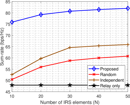
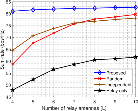
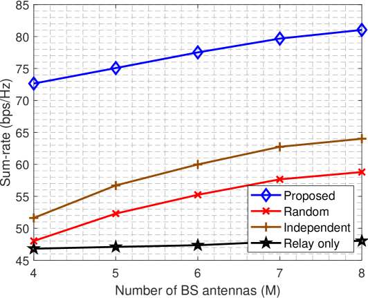
Fig. 2 compares the sum-rate performance vs. the number of IRS reflecting elements $N$, where we set $M=8$, $L=4$, and $K=4$. As can be seen, the sum-rate of all schemes except the Relay only scheme increases as $N$ increases. The proposed scheme outperforms all benchmarks since it fully exploits the coexistence system with optimized beamforming and transmission mechanism. The Independent scheme exhibits performance loss in comparison to the proposed scheme since IRS is turned off in the second phase and thus relaying in the second phase does not acquire performance gain from IRS-enhanced links and IRS beamforming. This suggests that the interaction between IRS and DF relay benefits the system sum-rate. Comparing the Independent and Random schemes, while the Independent scheme only leverages IRS in the first phase, it still outperforms the Random scheme with IRS operating in both phases. This is because, while the Independent scheme achieves a lower SINR in the second phase as compared to the Random scheme, it provides a much higher SINR in the first phase due to judicious IRS beamforming, resulting in an overall higher sum-rate. The Random scheme outperforms the Relay only scheme since IRS, even with random phase shifts, provides additional paths for transmission.

Fig. 2 compares the sum-rate performance vs. the number of relay antennas $L$, where we set $M=8$, $N=30$, and $K=4$. The sum-rate of all schemes increases with $L$ due to a higher degree of freedom in the second phase. The proposed scheme achieves the best sum-rate performance in all antenna configurations, with diminishing gains as $L$ increases. This is because the existence and optimization of IRS with $N=30$ reflecting elements dominates the change in $L$ in terms of the system capacity in the second phase. As a result, increasing the number of relay antennas brings relatively small merits to the proposed scheme. The Independent and Random schemes exhibit a crossing point; specifically, the Random scheme outperforms the Independent scheme in the larger $L$ regime. The reason is that the DF relay with more antennas can better adjust the relay beamforming vectors $\{{\mathbf{f}}_{k}\}$ in (6) for the combined IRS-assisted and direct channels from the relay to end users in the Random scheme. In contrast, since the IRS is turned off in the second phase, a relatively small gain is created for the Independent scheme as $L$ increases. More specifically, the higher SINR in the second phase outweighs the lower SINR in the first phase for the Random scheme, as compared to the Independent scheme.

Fig. 2 plots the sum-rate performance vs. the number of BS antennas $M$, where we set $L=4$, $N=30$, and $K=4$. The performance of all schemes improves as $M$ increases. Increasing $M$ however creates an incremental gain for the Relay only scheme due to the weak direct link from the BS to the end users. Other schemes, in contrast, are supported by the combined IRS-assisted and direct links in the first phase instead of only the direct link, and therefore observe larger gains as $M$ increases. The Independent scheme outperforms the Random scheme because the Independent scheme is enhanced by IRS beamforming in the first phase. Without optimized IRS phase shifts, the Random scheme suffers from performance loss. Especially, in the small $M$ region, the Random scheme achieves only a small performance gain as compared to the Relay only scheme. This suggests that the coexistence of an IRS and a relay does not always significantly benefit communications unless a proper co-design is performed.

References

- [1] Q. Wu and R. Zhang, “Towards smart and reconfigurable environment: Intelligent reflecting surface aided wireless network,” IEEE Commun. Mag., vol. 58, no. 1, pp. 106–112, Jan. 2020.
- [2] M. Di Renzo, A. Zappone, M. Debbah, M.-S. Alouini, C. Yuen, J. de Rosny, and S. Tretyakov, “Smart radio environments empowered by reconfigurable intelligent surfaces: How it works, state of research, and the road ahead,” IEEE J. Sel. Areas Commun., vol. 38, no. 11, pp. 2450–2525, Nov. 2020.
- [3] Q. Wu and R. Zhang, “Intelligent reflecting surface enhanced wireless network: Joint active and passive beamforming design,” in Proc. IEEE GLOBECOM, 2018, pp. 1–6.
- [4] C. Huang, A. Zappone, M. Debbah, and C. Yuen, “Achievable rate maximization by passive intelligent mirrors,” in Proc. IEEE ICASSP, 2018, pp. 3714–3718.
- [5] C. Huang, R. Mo, and C. Yuen, “Reconfigurable intelligent surface assisted multiuser MISO systems exploiting deep reinforcement learning,” IEEE J. Sel. Areas Commun., vol. 38, no. 8, pp. 1839–1850, Aug. 2020.
- [6] H. Li, R. Liu, M. Liy, Q. Liu, and X. Li, “IRS-enhanced wideband MU-MISO-OFDM communication systems,” in Proc. IEEE WCNC, 2020, pp. 1–6.
- [7] X. Mu, Y. Liu, L. Guo, J. Lin, and N. Al-Dhahir, “Exploiting intelligent reflecting surfaces in NOMA networks: Joint beamforming optimization,” IEEE Trans. Wireless Commun., vol. 19, no. 10, pp. 6884–6898, Oct. 2020.
- [8] Q. Wu and R. Zhang, “Intelligent reflecting surface enhanced wireless network via joint active and passive beamforming,” IEEE Trans. Wireless Commun., vol. 18, no. 11, pp. 5394–5409, Nov. 2019.
- [9] B. Zheng, Q. Wu, and R. Zhang, “Intelligent reflecting surface-assisted multiple access with user pairing: NOMA or OMA?” IEEE Commun. Lett., vol. 24, no. 4, pp. 753–757, Apr. 2020.
- [10] E. Björnson, Ö. Özdogan, and E. G. Larsson, “Intelligent reflecting surface versus decode-and-forward: How large surfaces are needed to beat relaying?” IEEE Wireless Commun. Lett., vol. 9, no. 2, pp. 244–248, Feb. 2020.
- [11] C. Huang, A. Zappone, G. C. Alexandropoulos, M. Debbah, and C. Yuen, “Reconfigurable intelligent surfaces for energy efficiency in wireless communication,” IEEE Trans. Wireless Commun., vol. 18, no. 8, pp. 4157–4170, Aug. 2019.
- [12] Q.-U.-A. Nadeem, A. Kammoun, A. Chaaban, M. Debbah, and M.-S. Alouini, “Asymptotic max-min SINR analysis of reconfigurable intelligent surface assisted MISO systems,” IEEE Trans. Wireless Commun., vol. 19, no. 12, pp. 7748–7764, Dec. 2020.
- [13] M. Di Renzo, K. Ntontin, J. Song, F. H. Danufane, X. Qian, F. Lazarakis, J. De Rosny, D.-T. Phan-Huy, O. Simeone, R. Zhang, M. Debbah, G. Lerosey, M. Fink, S. Tretyakov, and S. Shamai, “Reconfigurable intelligent surfaces vs. relaying: Differences, similarities, and performance comparison,” IEEE Open J. Commun. Soc., vol. 1, pp. 798–807, 2020.
- [14] I. Yildirim, F. Kilinc, E. Basar, and G. C. Alexandropoulos, “Hybrid RIS-empowered reflection and decode-and-forward relaying for coverage extension,” IEEE Commun. Lett., vol. 25, no. 5, pp. 1692–1696, May 2021.
- [15] D. Tse and P. Viswanath, Fundamentals of Wireless Communication. Cambridge, U.K.: Cambridge Univ. Press, 2005.
- [16] M. Grant and S. Boyd, “CVX: Matlab software for disciplined convex programming, version 2.1,” http://cvxr.com/cvx, Mar. 2014.
- [17] Y. Huang and D. P. Palomar, “Randomized algorithms for optimal solutions of double-sided QCQP with applications in signal processing,” IEEE Trans. Signal Process., vol. 62, no. 5, pp. 1093–1108, Mar. 2014.