Interacted two-stage least squares with treatment effect heterogeneity

1 Introduction

Two-stage least squares (2sls) is widely used for estimating treatment effects when instrumental variables (IVs) are available for endogenous treatments. Under the potential outcomes framework, Imbens and Angrist (1994) and Angrist et al. (1996) defined the local average treatment effect (LATE) as the average treatment effect over the subpopulation of compliers whose treatment status is affected by the IV, and formalized the assumptions on the IV that ensure the consistency of 2sls for estimating the LATE.

Often, IVs only satisfy the IV assumptions after conditioning on a set of covariates. Refer to such IVs as conditionally valid IVs hence. A common strategy is to include the corresponding covariates as additional regressors when fitting the 2sls. When treatment effect heterogeneity with regard to covariates is suspected, an intuitive generalization, which we term the interacted 2sls, is to add the IV-covariate and treatment-covariate interactions to the first and second stages, respectively (Angrist and Pischke, 2009, Section 4.5.2).

To our knowledge, theoretical properties of the interacted 2sls have not been discussed under the LATE framework except when the IV is randomly assigned hence unconditionally valid (Ding et al., 2019). Our paper closes this gap and clarifies the properties of the interacted 2sls in the more prevalent setting where the IV is conditionally valid.

Our contributions are threefold. First, we show that the interacted 2sls with centered covariates is consistent for estimating the LATE if either of the following conditions holds:

(i)

the IV-covariate interactions are linear in the covariates;
(ii)

the linear outcome model underlying the interacted 2sls is correct.

In particular, condition (i) is satisfied if either (ia) the covariates are categorical or (ib) the IV is randomly assigned. In contrast, existing 2sls procedures with an additive second stage only recover weighted averages of the conditional LATEs that generally differ from the LATE (Angrist and Imbens, 1995; Sloczynski, 2022; Blandhol et al., 2022). This illustrates an advantage of including treatment-covariate interactions in the second stage.

Second, define systematic treatment effect variation as the variation in individual treatment effects that can be explained by covariates (Heckman et al., 1997; Djebbari and Smith, 2008). We show that the coefficients of the treatment-covariate interactions from the interacted 2sls are consistent for estimating the systematic treatment effect variation among compliers if either condition (i) or condition (ii) holds. Furthermore, we connect the 2sls estimator with the weighting perspective in Abadie (2003), and establish the necessity of condition (i) in the absence of additional assumptions on the outcome model. The results extend the literature on the connection between regression and weighting for estimating the average treatment effect and LATE (Kline, 2011; Chattopadhyay and Zubizarreta, 2023; Chattopadhyay et al., 2024; Słoczyński et al., 2025; frolich2007nonparametric).

Third, to remedy the possible biases when neither condition (i) nor condition (ii) holds, we propose stratifying based on the estimated propensity score of the IV and using the stratum dummies as the new covariates to fit the interacted 2sls. While propensity score stratification is standard for estimating the average treatment effect (Rosenbaum and Rubin, 1983) and LATE (Cheng and Lin, 2018; Pashley et al., 2024), we highlight its value in approximating treatment effect heterogeneity with respect to the IV propensity score.

Notation.

For a set of tuples $\{(u_{i},v_{i1},\ldots,v_{iL}):i=1,\ldots,N\}$ with $u_{i}\in\mathbb{R}^{K}$ and $v_{il}\in\mathbb{R}^{K_{l}}$ for $l=1,\ldots,L$ , denote by $\texttt{lm}(u_{i}\sim v_{i1}+\cdots+v_{iL})$ the least squares fit of the component-wise linear regression of $u_{i}$ on $(v_{i1}^{\top},\ldots,v_{iL}^{\top})^{\top}$ . We allow each $v_{il}$ to be a scalar or a vector and use + to denote concatenation of regressors. Throughout, we focus on the numeric outputs of least squares without invoking any assumption of the corresponding linear model. For two random vectors $Y\in\mathbb{R}^{p}$ and $X\in\mathbb{R}^{q}$ , denote by $\textup{proj}(Y\mid X)$ the linear projection of $Y$ on $X$ in that $\textup{proj}(Y\mid X)=BX$ , where $B=\textup{argmin}_{b\in\mathbb{R}^{p\times q}}\mathbb{E}\{(Y-bX)^{2}\}=\mathbb{E}(YX^{\top})\{\mathbb{E}(XX^{\top})\}^{-1}$ . Let $1(\cdot)$ denote the indicator function. Let $\perp\!\!\!\perp$ denote independence.

2 Interacted 2SLS and identifying assumptions

2.1 Interacted 2SLS

Consider a study with two treatment levels, indexed by $d=0,1$ , and a study population of $N$ units, indexed by $i=1,\ldots,N$ . For each unit, we observe a treatment status $D_{i}\in\{0,1\}$ , an outcome of interest $Y_{i}\in\mathbb{R}$ , a baseline covariate vector $X_{i}\in\mathbb{R}^{K}$ , and a binary IV $Z_{i}\in\{0,1\}$ that is valid conditional on $X_{i}$ . We assume $X_{i}=(1,X_{i1},\ldots,X_{i,K-1})^{\top}$ includes the constant one as the first element unless specified otherwise, and state the IV assumptions in Section 2.2. Let $\mathbb{E}(Z_{i}\mid X_{i})=\mathbb{P}(Z_{i}=1\mid X_{i})$ denote the IV propensity score of unit $i$ (Rosenbaum and Rubin, 1983).

Definition 1 below reviews the standard 2sls procedure for estimating the causal effect of the treatment on outcome. We call it the additive 2sls to signify the additive regression specifications in both stages.

Definition 1 (Additive 2sls).

(i)

First stage: Fit $\texttt{lm}(D_{i}\sim Z_{i}+X_{i})$ over $i=1,\ldots,N$ . Denote the fitted values by $\hat{D}_{i}$ for $i=1,\ldots,N$ .
(ii)

Second stage: Fit $\texttt{lm}(Y_{i}\sim\hat{D}_{i}+X_{i})$ over $i=1,\ldots,N$ . Estimate the treatment effect by the coefficient of $\hat{D}_{i}$ .

The standard 2sls in Definition 1 is motivated by the additive working model $Y_{i}=D_{i}\beta_{D}+X_{i}^{\top}\beta_{X}+\eta_{i}$ , where $\mathbb{E}(\eta_{i}\mid Z_{i},X_{i})=0$ . The coefficient of $D_{i}$ , $\beta_{D}$ , is the constant treatment effect of interest, and we use $Z_{i}$ to instrument the possibly endogenous $D_{i}$ . We use the term working model to refer to models that are used to construct estimators but not necessarily correct.

When treatment effect heterogeneity with regard to covariates is suspected, an intuitive generalization is to consider the interacted working model

\displaystyle Y_{i}=D_{i}X_{i}^{\top}\beta_{DX}+X_{i}^{\top}\beta_{X}+\eta_{i},\quad\text{where \ $\mathbb{E}(\eta_{i}\mid Z_{i},X_{i})=0$,}

(1)

with $X_{i}^{\top}\beta_{DX}$ representing the covariate-dependent treatment effect. We can then use $Z_{i}X_{i}$ to instrument the possibly endogenous $D_{i}X_{i}$ ; see, e.g., Angrist and Pischke (2009, Section 4.5.2). We term the resulting 2sls procedure the interacted 2sls, formalized in Definition 2 below.

Definition 2 (Interacted 2sls).

(i)

First stage: Fit $\texttt{lm}(D_{i}X_{i}\sim Z_{i}X_{i}+X_{i})$ over $i=1,\ldots,N$ , as the component-wise regression of $D_{i}X_{i}$ on $(Z_{i}X_{i}^{\top},X_{i}^{\top})^{\top}$ . Denote the fitted values by $\widehat{DX}_{i}$ for $i=1,\ldots,N$ .
(ii)

Second stage: Fit $\texttt{lm}(Y_{i}\sim\widehat{DX}_{i}+X_{i})$ over $i=1,\ldots,N$ . Let $\hat{\beta}_{\textsc{2sls}}$ denote the coefficient vector of $\widehat{DX}_{i}$ .

Of interest is the causal interpretation of the coefficient vector $\hat{\beta}_{\textsc{2sls}}$ .

2.2 IV assumptions and causal estimands

We formalize below the IV assumptions and corresponding causal estimands using the potential outcomes framework (Imbens and Angrist, 1994; Angrist et al., 1996).

For $z,d\in\{0,1\}$ , let $D_{i}(z)$ denote the potential treatment status of unit $i$ if $Z_{i}=z$ , and let $Y_{i}(z,d)$ denote the potential outcome of unit $i$ if $Z_{i}=z$ and $D_{i}=d$ . The observed treatment status and outcome satisfy $D_{i}=D_{i}(Z_{i})$ and $Y_{i}=Y_{i}(Z_{i},D_{i})=Y_{i}(Z_{i},D_{i}(Z_{i}))$ .

Following the literature, we classify the units into four compliance types, denoted by $U_{i}$ , based on the joint values of $D_{i}(1)$ and $D_{i}(0)$ . We call unit $i$ an always-taker if $D_{i}(1)=D_{i}(0)=1$ , denoted by $U_{i}=\textup{a}$ ; a complier if $D_{i}(1)=1$ and $D_{i}(0)=0$ , denoted by $U_{i}=\textup{c}$ ; a defier if $D_{i}(1)=0$ and $D_{i}(0)=1$ , denoted by $U_{i}=\textup{d}$ ; and a never-taker if $D_{i}(1)=D_{i}(0)=0$ , denoted by $U_{i}=\textup{n}$ .

Assumption 1 below reviews the assumptions for conditionally valid IVs that we assume throughout the paper.

Assumption 1.

$\{Y_{i}(z,d),D_{i}(z),X_{i},Z_{i}:z=0,1;\ d=0,1\}$ are independent and identically distributed across $i=1,\ldots,N$ , and satisfy the following conditions:

(i)

Selection on observables: $Z_{i}\perp\!\!\!\perp\{Y_{i}(z,d),D_{i}(z):z=0,1;\,d=0,1\}\mid X_{i}$ .
(ii)

Overlap: $0<\mathbb{E}(Z_{i}\mid X_{i})<1$ .
(iii)

Exclusion restriction: $Y_{i}(0,d)=Y_{i}(1,d)=Y_{i}(d)$ for $d=0,1$ , where $Y_{i}(d)$ denotes the common value.
(iv)

Relevance: $\mathbb{E}\{D_{i}(1)-D_{i}(0)\mid X_{i}\}\neq 0$ .
(v)

Monotonicity: $D_{i}(1)\geq D_{i}(0)$ .

Assumption 1(i) ensures $Z_{i}$ is as-if randomly assigned given $X_{i}$ . Assumption 1(ii) ensures positive probabilities of $Z_{i}=1$ and $Z_{i}=0$ at all possible values of $X_{i}$ . Assumption 1(iii) ensures $Z_{i}$ has no effect on the outcome once we condition on the treatment status. Assumption 1(iv) ensures $Z_{i}$ has a nonzero causal effect on the treatment status at all possible values of $X_{i}$ . Assumption 1(v) precludes defiers. Assumption 1(iv)–(v) together ensure positive proportion of compliers at all possible values of $X_{i}$ , i.e., $\mathbb{P}(U_{i}=\textup{c}\mid X_{i})>0$ .

Recall $Y_{i}(d)$ as the common value of $Y_{i}(1,d)=Y_{i}(0,d)$ for $d=0,1$ under Assumption 1(iii). Define $\tau_{i}=Y_{i}(1)-Y_{i}(0)$ as the individual treatment effect of unit $i$ . Define

\displaystyle\tau_{\textup{c}}=\mathbb{E}(\tau_{i}\mid U_{i}=\textup{c})

(2)

as the local average treatment effect (LATE) on compliers, and define

\displaystyle\tau_{\textup{c}}(X_{i})=\mathbb{E}(\tau_{i}\mid X_{i},\,U_{i}=\textup{c})

(3)

as the conditional LATE given $X_{i}$ . The law of iterated expectations ensures $\tau_{\textup{c}}=\mathbb{E}\left\{\tau_{\textup{c}}(X_{i})\mid U_{i}=\textup{c}\right\}$ .

To quantify treatment effect heterogeneity with regard to covariates, consider the linear projection of $\tau_{i}$ on $X_{i}$ among compliers, denoted by $\textup{proj}_{\,U_{i}=\textup{c}}(\tau_{i}\mid X_{i})=X_{i}^{\top}\beta_{\textup{c}}$ . The coefficient vector equals

\displaystyle\beta_{\textup{c}}=\textup{argmin}_{b\in\mathbb{R}^{K}}\mathbb{E}\left\{(\tau_{i}-X_{i}^{\top}b)^{2}\mid U_{i}=\textup{c}\right\}=\left\{\mathbb{E}(X_{i}X_{i}^{\top}\mid U_{i}=\textup{c})\right\}^{-1}\mathbb{E}\left(X_{i}\tau_{i}\mid U_{i}=\textup{c}\right).

(4)

By Angrist and Pischke (2009, Theorem 3.1.6), $X_{i}^{\top}\beta_{\textup{c}}$ is also the linear projection of the conditional LATE $\tau_{\textup{c}}(X_{i})$ on $X_{i}$ among compliers with $\beta_{\textup{c}}=\textup{argmin}_{b\in\mathbb{R}^{K}}\mathbb{E}[\{\tau_{\textup{c}}(X_{i})-X_{i}^{\top}b\}^{2}\mid U_{i}=\textup{c}]$ . This ensures $X_{i}^{\top}\beta_{\textup{c}}$ is the best linear approximation to both $\tau_{i}$ and $\tau_{\textup{c}}(X_{i})$ based on $X_{i}$ , generalizing the idea of systematic treatment effect variation in Djebbari and Smith (2008) to the IV setting; see also Heckman et al. (1997). We define $\beta_{\textup{c}}$ as the causal estimand for quantifying treatment effect heterogeneity among compliers that is explained by $X_{i}$ .

Recall $\hat{\beta}_{\textsc{2sls}}$ as the coefficient vector from the interacted 2sls in Definition 2. Under the finite-population, design-based framework, Ding et al. (2019) showed that $\hat{\beta}_{\textsc{2sls}}$ is consistent for estimating $\beta_{\textup{c}}$ when $Z_{i}$ is randomly assigned hence valid without conditioning on $X_{i}$ . We establish in Section 3 the properties of $\hat{\beta}_{\textsc{2sls}}$ for estimating $\tau_{\textup{c}}$ , $\tau_{\textup{c}}(X_{i})$ , and $\beta_{\textup{c}}$ in the more prevalent setting where $Z_{i}$ is only conditionally valid given $X_{i}$ .

2.3 Identifying assumptions

We introduce below two assumptions central to our identification results. First, Assumption 2 below restricts the functional form of the IV propensity score, requiring the product of $\mathbb{E}(Z_{i}\mid X_{i})$ and $X_{i}$ to be linear in $X_{i}$ .

Assumption 2 (Linear IV-covariate interactions).

$\mathbb{E}(Z_{i}X_{i}\mid X_{i})$ is linear in $X_{i}$ .

In contrast, Assumption 3 below imposes linearity on the outcome model.

Assumption 3 (Correct interacted outcome model).

The interacted working model (1) is correct.

Proposition 1 below states three implications of Assumptions 2–3.

Proposition 1.

Let $K$ denote the dimension of the covariate vector $X_{i}$ .

(i)
Assumption 2 holds if either of the following conditions holds
1. (a)
  
  Categorical covariates: $X_{i}$ is categorical with $K$ levels.
2. (b)
  
  Random assignment of IV: $Z_{i}\perp\!\!\!\perp X_{i}$ .
(ii)

If Assumption 2 holds, then $\mathbb{E}(Z_{i}\mid X_{i})$ takes at most $K$ distinct values across all possible values of $X_{i}$ . If Assumption 2 holds for all possible assignment mechanisms of $Z_{i}$ , then $X_{i}$ is categorical with $K$ levels.

(iii)

Assume Assumption 1. Assumption 3 holds if the potential outcomes satisfy

\displaystyle\begin{array}[]{l}\mathbb{E}\{Y_{i}(1)\mid X_{i},U_{i}=\textup{a}\}=\mathbb{E}\{Y_{i}(1)\mid X_{i},U_{i}=\textup{c}\}=X_{i}^{\top}\beta_{1},\\ \mathbb{E}\{Y_{i}(0)\mid X_{i},U_{i}=\textup{n}\}=\mathbb{E}\{Y_{i}(0)\mid X_{i},U_{i}=\textup{c}\}=X_{i}^{\top}\beta_{0}\end{array}

for some fixed $\beta_{0},\beta_{1}\in\mathbb{R}^{K}$ .

Proposition 1(i) provides two important special cases of Assumption 2. Together with Assumption 1, the condition of $Z_{i}\perp\!\!\!\perp X_{i}$ in Proposition 1(ib) ensures the IV is valid without conditioning on $X_{i}$ .

Proposition 1(ii) ensures that the IV propensity score takes at most $K$ distinct values under Assumption 2. This substantially restricts the possible IV assignment mechanisms beyond the two special cases in Proposition 1(i).

Proposition 1(iii) provides a special case of Assumption 3 where the potential outcomes are linear in the covariates.

3 Identification by interacted 2SLS

We establish in this section the conditions for the interacted 2sls to recover the LATE and treatment effect heterogeneity with regard to covariates in the presence of treatment effect heterogeneity.

3.1 Identification of LATE

We first establish the properties of the interacted 2sls for estimating the LATE and unify the results with the literature. Assume throughout this subsection that $X_{i}=(1,X_{i1},\ldots,X_{i,K-1})^{\top}$ has the constant one as the first element.

3.1.1 Interacted 2SLS with centered covariates

Let $\mu_{k}=\mathbb{E}(X_{ik}\mid U_{i}=\textup{c})$ denote the complier average of $X_{ik}$ for $k=1,\ldots,K-1$ . While $\mu_{k}$ is generally unknown, we can consistently estimate it by the method of moments proposed by Imbens and Rubin (1997) or the weighted estimator proposed by Abadie (2003). Definition 3 below formalizes our proposed estimator of the LATE.

Definition 3.

Given $X_{i}=(1,X_{i1},\ldots,X_{i,K-1})^{\top}$ , let $\hat{\mu}_{k}$ be a consistent estimate of $\mu_{k}=\mathbb{E}(X_{ik}\mid U_{i}=\textup{c})$ for $k=1,\ldots,K-1$ . Let $\hat{\tau}_{\times\times}$ be the first element of $\hat{\beta}_{\textsc{2sls}}$ from the interacted 2sls in Definition 2 that uses $X_{i}^{0}=(1,X_{i1}-\hat{\mu}_{1},\ldots,X_{i,K-1}-\hat{\mu}_{K-1})^{\top}$ as the covariate vector.

We use the subscript $\times\times$ to signify the interacted first and second stages in the interacted 2sls. Given $D_{i}X_{i}^{0}=(D_{i},D_{i}(X_{i1}-\hat{\mu}_{1}),\ldots D_{i}(X_{i,K-1}-\hat{\mu}_{K-1}))^{\top}$ , $\hat{\tau}_{\times\times}$ is the coefficient of the fitted value of $D_{i}$ from the interacted second stage. Let $\tau_{\times\times}$ denote the probability limit of $\hat{\tau}_{\times\times}$ as the sample size $N$ goes to infinity. Theorem 1 below establishes the conditions for $\tau_{\times\times}$ to identify the LATE.

Theorem 1.

Assume Assumption 1. Then $\tau_{\times\times}=\tau_{\textup{c}}$ if either Assumption 2 or Assumption 3 holds.

Theorem 1 ensures the consistency of $\hat{\tau}_{\times\times}$ for estimating the LATE when either Assumption 2 or Assumption 3 holds. From Proposition 1, this encompasses (i) categorical covariates, (ii) unconditionally valid IV, and (iii) correct interacted working model as three special cases. In particular, the regression specification of the interacted 2sls is saturated when $X_{i}$ is categorical, and is therefore a special case of the saturated 2sls discussed by Blandhol et al. (2022).

Recall that $\hat{\tau}_{\times\times}$ is the first element of $\hat{\beta}_{\textsc{2sls}}$ with centered covariates. We provide intuition for the use of centered covariates in Section 3.2 after presenting the more general theory for $\hat{\beta}_{\textsc{2sls}}$ , and demonstrate the sufficiency of Assumptions 2 and 3 in Section 4. See Hirano and Imbens (2001) and Lin (2013) for similar uses of centered covariates when using interacted regression to estimate the average treatment effect.

Note that when computing $\hat{\tau}_{\times\times}$ , we use the estimated complier averages to center the covariates, because the true values are unknown. To conduct inference based on $\hat{\tau}_{\times\times}$ , we need to account for the uncertainty in estimating the complier means. This can be achieved by bootstrapping.

3.1.2 Unification with the literature

Theorem 1 contributes to the literature on using 2sls to estimate the LATE in the presence of treatment effect heterogeneity. Previously, Angrist and Imbens (1995) studied a variant of the additive 2sls in Definition 1 for categorical $X_{i}$ , and showed that the coefficient of $\hat{D}_{i}$ recovers a weighted average of the conditional LATEs that generally differs from $\tau_{\textup{c}}$ . Sloczynski (2022) studied the additive 2sls in Definition 1, and showed that when $\mathbb{E}(Z_{i}\mid X_{i})$ is linear in $X_{i}$ , the coefficient of $\hat{D}_{i}$ recovers a weighted average of the conditional LATEs that generally differs from $\tau_{\textup{c}}$ . Blandhol et al. (2022) studied the additive 2sls and showed that the coefficient of $\hat{D}_{i}$ recovers a weighted average of the conditional LATEs when the additive first stage is correctly specified, or saturated. In contrast, Theorem 1 ensures that the interacted 2sls directly recovers $\tau_{\textup{c}}$ if either (i) the covariates are categorical, or (ii) the IV is unconditionally valid, or (iii) the interacted working model (1) is correct. This illustrates an advantage of including the treatment-covariate interactions in the second stage.

We formalize the above overview in Definition 4 and Proposition 2 below. First, Definition 4 states the 2sls procedure considered by Angrist and Imbens (1995) and Sloczynski (2022).

Definition 4 (Interacted-additive 2sls).

(i)

First stage: Fit $\texttt{lm}(D_{i}\sim Z_{i}X_{i}+X_{i})$ over $i=1,\ldots,N$ . Denote the fitted values by $\hat{D}_{i}$ for $i=1,\ldots,N$ .
(ii)

Second stage: Fit $\texttt{lm}(Y_{i}\sim\hat{D}_{i}+X_{i})$ over $i=1,\ldots,N$ . Estimate the treatment effect by the coefficient of $\hat{D}_{i}$ , denoted by $\hat{\tau}_{\times+}$ .

We use the subscript $\times+$ to signify the interacted first stage and additive second stage. The additive, interacted, and interacted-additive 2sls in Definitions 1–2 and 4 are three variants of 2sls discussed in the LATE literature, summarized in Table 1. The combination of additive first stage and interacted second stage leads to degenerate second stage and is hence omitted.

Let $\hat{\tau}_{++}$ denote the coefficient of $\hat{D}_{i}$ from the additive 2sls in Definition 1. Let $\tau_{++}$ and $\tau_{\times+}$ denote the probability limits of $\hat{\tau}_{++}$ and $\hat{\tau}_{\times+}$ , respectively. Proposition 2 below states the conditions for $\tau_{++}$ and $\tau_{\times+}$ to identify a weighted average of $\tau_{\textup{c}}(X_{i})$ , and contrasts the results with that of $\tau_{\times\times}$ .

Let

\displaystyle w(X_{i})=\dfrac{\operatorname{var}\{\mathbb{E}(D_{i}\mid Z_{i},X_{i})\mid X_{i}\}}{\mathbb{E}\big{[}\operatorname{var}\{\mathbb{E}(D_{i}\mid Z_{i},X_{i})\mid X_{i}\}\big{]}}

with $w(X_{i})>0$ and $\mathbb{E}\{w(X_{i})\}=1$ . Let $\pi(X_{i})=\mathbb{P}(U_{i}=\textup{c}\mid X_{i})$ denote the proportion of compliers given $X_{i}$ . Let $\tilde{\pi}(X_{i})$ denote the linear projection of $\pi(X_{i})$ on $X_{i}$ weighted by $\operatorname{var}(Z_{i}\mid X_{i})$ . That is, $\tilde{\pi}(X_{i})=a^{\top}X_{i}$ with $a=\mathbb{E}\{\operatorname{var}(Z_{i}\mid X_{i})\cdot X_{i}X_{i}^{\top}\}^{-1}\mathbb{E}\{\operatorname{var}(Z_{i}\mid X_{i})\cdot X_{i}\,\pi(X_{i})\}$ .

Proposition 2.

Assume Assumption 1.

(i)

If $\mathbb{E}(Z_{i}\mid X_{i})$ is linear in $X_{i}$ , then $\tau_{++}=\mathbb{E}\{w_{+}(X_{i})\cdot\tau_{\textup{c}}(X_{i})\}$ , where

\displaystyle w_{+}(X_{i})=\dfrac{\operatorname{var}(Z_{i}\mid X_{i})\cdot\pi(X_{i})}{\mathbb{E}\left\{\operatorname{var}(Z_{i}\mid X_{i})\cdot\pi(X_{i})\right\}}\quad\text{with \ \ $w_{+}(X_{i})>0$ and $\mathbb{E}\{w_{+}(X_{i})\}=1$.}

Further assume that $\mathbb{E}(D_{i}\mid Z_{i},X_{i})$ is linear in $(Z_{i},X_{i})$ , i.e., the additive first stage in Definition 1 is correctly specified. Then $w_{+}(X_{i})=w(X_{i})$ .

(ii)

If Assumption 2 holds, then $\tau_{\times+}=\mathbb{E}\{w_{\times}(X_{i})\cdot\tau_{\textup{c}}(X_{i})\}$ , where

\displaystyle w_{\times}(X_{i})=\dfrac{\operatorname{var}(Z_{i}\mid X_{i})\cdot\tilde{\pi}(X_{i})\cdot\pi(X_{i})}{\mathbb{E}\left\{\operatorname{var}(Z_{i}\mid X_{i})\cdot\tilde{\pi}(X_{i})^{2}\right\}}\quad\text{with}\ \ \mathbb{E}\{w_{\times}(X_{i})\}=1.

Further assume that $\mathbb{E}(D_{i}\mid Z_{i},X_{i})$ is linear in $(Z_{i}X_{i},X_{i})$ , i.e., the interacted first stage in Definition 4 is correctly specified. Then $w_{\times}(X_{i})=w(X_{i})$ .

(iii)

If Assumption 2 or Assumption 3 holds, then $\tau_{\times\times}=\tau_{\textup{c}}$ .

Proposition 2(i) reviews Sloczynski (2022, Corollary 3.4) and ensures that when the IV propensity score $\mathbb{E}(Z_{i}\mid X_{i})$ is linear in $X_{i}$ , $\hat{\tau}_{++}$ recovers a weighted average of $\tau_{\textup{c}}(X_{i})$ that generally differs from $\tau_{\textup{c}}$ . We further show that $w_{+}(X_{i})$ simplifies to $w(X_{i})$ when the additive first stage is correctly specified. See Sloczynski (2022) for a detailed discussion about the deviation of $\tau_{++}$ from $\tau_{\textup{c}}$ .

Proposition 2(ii) extends Angrist and Imbens (1995) on categorical covariates to general covariates, and ensures that when $\mathbb{E}(Z_{i}X_{i}\mid X_{i})$ is linear in $X_{i}$ , $\hat{\tau}_{\times+}$ recovers a weighted average of $\tau_{\textup{c}}(X_{i})$ that generally differs from $\tau_{\textup{c}}$ . A technical subtlety is that $w_{\times}(X_{i})$ may be negative due to $\tilde{\pi}(X_{i})$ , so that some $\tau_{\textup{c}}(X_{i})$ may be negatively weighted. Note that categorical covariates satisfy both Assumption 2 and the condition that $\mathbb{E}(D_{i}\mid Z_{i},X_{i})$ is linear in $(Z_{i}X_{i},X_{i})$ . Proposition 2(ii) then simplifies to the special case in Angrist and Imbens (1995).

Proposition 2(iii) follows from Theorem 1 and ensures that when $\mathbb{E}(Z_{i}X_{i}\mid X_{i})$ is linear in $X_{i}$ , $\hat{\tau}_{\times\times}$ from the interacted 2sls directly recovers $\tau_{\textup{c}}$ .

Together, Proposition 2 illustrates the advantage of $\hat{\tau}_{\times\times}$ over $\hat{\tau}_{\times+}$ and $\hat{\tau}_{++}$ for estimating the LATE, especially when the covariates are categorical or the IV is unconditionally valid; c.f. Proposition 1. See Table 1 for a summary and Section 6 for a simulated example.

Table 1: 2sls for estimating the LATE.

Second stage

First stage

Additive

Interacted

\texttt{lm}(Y_{i}\sim\hat{D}_{i}+X_{i})

\texttt{lm}(Y_{i}\sim\widehat{DX}_{i}+X_{i})

Additive

\texttt{lm}(D_{i}\sim Z_{i}+X_{i})

\hat{\tau}_{++}\overset{\mathbb{P}}{\to}\mathbb{E}\left\{w_{+}(X_{i})\cdot\tau_{\textup{c}}(X_{i})\right\}

if

\mathbb{E}(Z_{i}\mid X_{i})

is linear in

X_{i}

n.a.

Interacted

\texttt{lm}(D_{i}\sim Z_{i}X_{i}+X_{i})

or

\texttt{lm}(D_{i}X_{i}\sim Z_{i}X_{i}+X_{i})

\hat{\tau}_{\times+}\overset{\mathbb{P}}{\to}\mathbb{E}\left\{w_{\times}(X_{i})\cdot\tau_{\textup{c}}(X_{i})\right\}

if Assumption 2 holds

\hat{\tau}_{\times\times}\overset{\mathbb{P}}{\to}\tau_{\textup{c}}

if

if Assumption 2 or

Assumption 3 holds

Note. $\hat{\tau}_{++}$ denotes the coefficient of $\hat{D}_{i}$ from the additive 2sls in Definition 1. $\hat{\tau}_{\times+}$ denotes the coefficient of $\hat{D}_{i}$ from the interacted-additive 2sls in Definition 4. $\hat{\tau}_{\times\times}$ denotes the coefficient of $\hat{D}_{i}$ from the interacted 2sls with centered covariates in Definition 3. $w_{+}(X_{i})$ and $w_{\times}(X_{i})$ are defined in Proposition 2.

3.2 Identification of treatment effect heterogeneity

We establish in this subsection the properties of the interacted 2sls for estimating $\beta_{\textup{c}}$ that quantifies treatment effect heterogeneity with regard to covariates. Recall $\hat{\beta}_{\textsc{2sls}}$ as the coefficient vector of $D_{i}X_{i}$ from the interacted 2sls in Definition 2. Let $\beta_{\textsc{2sls}}$ denote the probability limit of $\hat{\beta}_{\textsc{2sls}}$ .

3.2.1 General theory

Let $\textup{proj}(D_{i}X_{i}\mid Z_{i}X_{i},X_{i})$ denote the linear projection of $D_{i}X_{i}$ on $(Z_{i}X_{i}^{\top},X_{i}^{\top})^{\top}$ . Let $\widetilde{DX}_{i}$ denote the residual from the linear projection of $\textup{proj}(D_{i}X_{i}\mid Z_{i}X_{i},X_{i})$ on $X_{i}$ . Let $\epsilon_{i}=\tau_{i}-X_{i}^{\top}\beta_{\textup{c}}$ for compliers, as the residual from the linear projection of $\tau_{i}$ on $X_{i}$ among compliers. Let $\Delta_{i}=Y_{i}(0)$ for compliers and never-takers, and $\Delta_{i}=Y_{i}(1)-X_{i}^{\top}\beta_{\textup{c}}$ for always-takers. Let

\displaystyle\begin{array}[]{lll}B_{1}&=&C_{1}\cdot\mathbb{E}\Big{[}\Big{\{}\mathbb{E}(Z_{i}X_{i}\mid X_{i})-\textup{proj}(Z_{i}X_{i}\mid X_{i})\Big{\}}\cdot\Big{\{}\mathbb{E}(\Delta_{i}\mid X_{i})-\textup{proj}(\Delta_{i}\mid X_{i})\Big{\}}\Big{]},\\ B_{2}&=&C_{1}(I_{K}-C_{2})\cdot\mathbb{E}\Big{\{}\mathbb{E}(Z_{i}X_{i}\mid X_{i})\cdot\epsilon_{i}\mid U_{i}=\textup{c}\Big{\}}\cdot\mathbb{P}(U_{i}=\textup{c}),\end{array}

(8)

where $C_{1}$ is the coefficient matrix of $Z_{i}X_{i}$ in $\textup{proj}(D_{i}X_{i}\mid Z_{i}X_{i},X_{i})$ and $C_{2}$ is the coefficient matrix of $X_{i}$ in $\textup{proj}(Z_{i}X_{i}\mid X_{i})$ .

Theorem 2.

Assume Assumption 1. Then $\beta_{\textsc{2sls}}=\beta_{\textup{c}}+\{\mathbb{E}(\widetilde{DX}_{i}\cdot\widetilde{DX}_{i}^{\top})\}^{-1}(B_{1}+B_{2})$ , where $B_{1}=B_{2}=0$ if either Assumption 2 or Assumption 3 holds.

Theorem 2 ensures that $\beta_{\textsc{2sls}}$ identifies $\beta_{\textup{c}}$ if and only if $B_{1}+B_{2}=0$ , and establishes Assumption 2 and Assumption 3 as two sufficient conditions. We discuss the sufficiency and “almost necessity” of these two assumptions in Section 4.

Recall that Assumption 2 holds when the IV is randomly assigned. Therefore, Theorem 2 ensures $\beta_{\textsc{2sls}}=\beta_{\textup{c}}$ for randomly assigned IVs as a special case. See Ding et al. (2019, Theorem 7) for similar results in the finite-population, design-based framework.

In addition, recall that Assumption 2 holds when the covariates are categorical. Therefore, Theorem 2 ensures $\beta_{\textsc{2sls}}=\beta_{\textup{c}}$ for categorical covariates. As it turns out, the elements of $\beta_{\textup{c}}$ equal the category-specific LATEs if we define $X_{i}$ as the vector of all category dummies, without the constant one. This allows us to recover the conditional LATEs as coefficients of the interacted 2sls for categorical covariates. We formalize the intuition below.

3.2.2 The special case of categorical covariates

Assume throughout this subsection that the covariate vector $X_{i}$ encodes a $K$ -level categorical variable, represented by $X_{i}^{*}\in\{1,\ldots,K\}$ , using category dummies:

\displaystyle X_{i}=(1(X_{i}^{*}=1),\ldots,1(X_{i}^{*}=K))^{\top}.

(9)

Define

\displaystyle\tau_{[k]\textup{c}}=\mathbb{E}(\tau_{i}\mid X_{i}^{*}=k,\,U_{i}=\textup{c})

as the conditional LATE on compliers with $X_{i}^{*}=k$ ; c.f. Eq. (3). Lemma 1 below states the simplified forms of $\beta_{\textup{c}}$ and $\tau_{\textup{c}}(X_{i})$ under (9).

Lemma 1.

Assume (9). Then $\beta_{\textup{c}}=(\tau_{[1]\textup{c}},\ldots,\tau_{[K]\textup{c}})^{\top}$ and $\tau_{\textup{c}}(X_{i})=X_{i}^{\top}\beta_{\textup{c}}$ .

Lemma 1 has two implications. First, when $X_{i}$ is the dummy vector, the corresponding $\beta_{\textup{c}}$ has the subgroup LATEs $\tau_{[k]\textup{c}}$ ’s as its elements, which adds interpretability. Second, with categorical $X_{i}$ , the conditional LATE $\tau_{\textup{c}}(X_{i})$ is linear in $X_{i}$ and equals the linear projection $X_{i}^{\top}\beta_{\textup{c}}$ . This is not true for general $X_{i}$ , so that linear projection is only an approximation.

Corollary 1 below follows from Theorem 2 and Lemma 1, and ensures the coefficients of the interacted 2sls are consistent for estimating the conditional LATEs.

Corollary 1.

Assume Assumption 1 and (9). We have $\beta_{\textsc{2sls}}=(\tau_{[1]\textup{c}},\ldots,\tau_{[K]\textup{c}})^{\top}$ .

3.3 Reconciliation of Theorems 1 and 2

We now clarify the connection between Theorems 1 and 2, and provide intuition for the use of centered covariates in estimating the LATE.

Recall that $\hat{\tau}_{\times\times}$ is the first element of $\hat{\beta}_{\textsc{2sls}}$ with centered covariates. Theorem 2 ensures that $\hat{\beta}_{\textsc{2sls}}$ is consistent for estimating $\beta_{\textup{c}}$ when either Assumption 2 or Assumption 3 holds. Therefore, a logical basis for using $\hat{\tau}_{\times\times}$ to estimate $\tau_{\textup{c}}$ is that $\tau_{\textup{c}}$ equals the first element of $\beta_{\textup{c}}$ . Lemma 2 below ensures that this condition is satisfied when the nonconstant covariates are centered by their respective complier averages. This establishes Theorem 1 as a direct consequence of Theorem 2, and justifies the use of centered covariates for estimating the LATE.

Lemma 2.

Assume $X_{i}=(1,X_{i1},\ldots,X_{i,K-1})^{\top}$ . If $\mathbb{E}(X_{ik}\mid U_{i}=\textup{c})=0$ for $k=1,\ldots,K-1$ , then the first element of $\beta_{\textup{c}}$ equals $\tau_{\textup{c}}$ .

4 Discussion of Assumptions 2 and 3

We discuss in this section the sufficiency and “almost necessity” of Assumptions 2 and 3 to ensure $\beta_{\textsc{2sls}}=\beta_{\textup{c}}$ in Theorem 2.

4.1 Sufficiency and “almost necessity” of Assumption 2

We discuss below the sufficiency and “almost necessity” of Assumption 2. We first demonstrate the sufficiency of Assumption 2 to ensure $B_{1}=B_{2}=0$ , as a sufficient condition for $\beta_{\textsc{2sls}}=\beta_{\textup{c}}$ by Theorem 2. We then adopt the weighting perspective in Abadie (2003) and establish the necessity of Assumption 2 to ensure $\beta_{\textsc{2sls}}=\beta_{\textup{c}}$ in the absence of additional assumptions on the outcome model beyond Assumption 1.

4.1.1 Sufficiency

Recall the definitions of $B_{1}$ and $B_{2}$ from Eq. (8), where $C_{2}$ denotes the coefficient matrix of $X_{i}$ in $\textup{proj}(Z_{i}X_{i}\mid X_{i})$ . Assumption 2 ensures

\displaystyle\mathbb{E}(Z_{i}X_{i}\mid X_{i})=\textup{proj}(Z_{i}X_{i}\mid X_{i})=C_{2}X_{i}

(10)

so that $B_{1}=0$ .

In addition, recall that $\epsilon_{i}$ is the residual from the linear projection of $\tau_{i}$ on $X_{i}$ among compliers. Properties of linear projection ensure $\mathbb{E}(X_{i}\epsilon_{i}\mid U_{i}=\textup{c})=0$ so that the expectation term in $B_{2}$ satisfies

\displaystyle\mathbb{E}\Big{\{}\mathbb{E}(Z_{i}X_{i}\mid X_{i})\cdot\epsilon_{i}\mid U_{i}=\textup{c}\Big{\}}\overset{\eqref{eq:proj_assm2}}{=}\mathbb{E}(C_{2}X_{i}\epsilon_{i}\mid U_{i}=\textup{c})=0.

This ensures $B_{2}=0$ and therefore the sufficiency of Assumption 2 to ensure $B_{1}=B_{2}=0$ .

4.1.2 Necessity in the absence of additional assumptions on outcome model

Proposition 3 below expresses $\beta_{\textsc{2sls}}$ as a weighted estimator and establishes the necessity of Assumption 2 to ensure $\beta_{\textsc{2sls}}=\beta_{\textup{c}}$ in the absence of additional assumptions on the outcome model. Recall that $\widetilde{DX}_{i}$ denotes the residual from the linear projection of $\textup{proj}(D_{i}X_{i}\mid Z_{i}X_{i},X_{i})$ on $X_{i}$ .

Proposition 3.

(i)

$\beta_{\textsc{2sls}}=\mathbb{E}(w_{i}Y_{i})$ , where $w_{i}=\{\mathbb{E}(\widetilde{DX}_{i}\cdot\widetilde{DX}_{i}^{\top})\}^{-1}\widetilde{DX}_{i}.$

(ii)

Under Assumption 1, we have $\beta_{\textup{c}}=\mathbb{E}(u_{i}Y_{i})$ , where $u_{i}=\{\mathbb{E}(X_{i}X_{i}^{\top}\mid U_{i}=\textup{c})\}^{-1}\pi_{\textup{c}}^{-1}\Delta\kappa X_{i}$ with

\displaystyle\Delta\kappa=\dfrac{Z_{i}-\mathbb{E}(Z_{i}\mid X_{i})}{\mathbb{E}(Z_{i}\mid X_{i})\{1-\mathbb{E}(Z_{i}\mid X_{i})\}}.

(iii)

If $w_{i}=u_{i}$ , then Assumption 2 must hold.

Proposition 3(i) expresses $\beta_{\textsc{2sls}}$ as a weighted average of the outcome $Y_{i}$ . The result is numeric and does not require Assumption 1.

Proposition 3(ii) follows from Abadie (2003) and expresses $\beta_{\textup{c}}$ as a weighted average of $Y_{i}$ when Assumption 1 holds.

Proposition 3(iii) connects Proposition 3(i)–(ii) and establishes the necessity of Assumption 2 to ensure $w_{i}=u_{i}$ .

Together, Proposition 3(i)–(iii) establish the necessity of Assumption 2 to ensure $\beta_{\textsc{2sls}}=\beta_{\textup{c}}$ in the absence of additional assumptions on the outcome model.

4.2 Sufficiency and “almost necessity” of Assumption 3

We discuss below the sufficiency and “almost necessity” of Assumption 3 to ensure $B_{1}=B_{2}=0$ in the absence of additional assumptions on $Z_{i}$ beyond Assumption 1.

Without additional assumptions on $Z_{i}$ , the $\mathbb{E}(Z_{i}X_{i}\mid X_{i})$ in the definitions of $B_{1}$ and $B_{2}$ is arbitrary. To ensure $B_{1}=0$ , we generally need $\mathbb{E}(\Delta_{i}\mid X_{i})=\textup{proj}(\Delta_{i}\mid X_{i})$ , which is equivalent to

\mathbb{E}(\Delta_{i}\mid X_{i})

is linear in

X_{i}

.

(11)

In addition, Lemma S4 in the Supplementary Material ensures that $C_{1}(I_{K}-C_{2})$ is invertible. From Eq. (8), we have $B_{2}=0$ if and only if

\displaystyle\mathbb{E}\Big{\{}\mathbb{E}(Z_{i}X_{i}\mid X_{i})\cdot\epsilon_{i}\mid U_{i}=\textup{c}\Big{\}}=0.

(12)

By the law of iterated expectations, the left-hand side of condition (12) equals

	$\displaystyle\mathbb{E}\Big{\{}\mathbb{E}(Z_{i}X_{i}\mid X_{i})\cdot\epsilon_{i}\mid U_{i}=\textup{c}\Big{\}}$	$\displaystyle=$	$\displaystyle\mathbb{E}\Big{[}\mathbb{E}\Big{\{}\mathbb{E}(Z_{i}X_{i}\mid X_{i})\cdot\epsilon_{i}\mid X_{i},U_{i}=\textup{c}\Big{\}}\mid U_{i}=\textup{c}\Big{]}$
		$\displaystyle=$	$\displaystyle\mathbb{E}\Big{[}\mathbb{E}(Z_{i}X_{i}\mid X_{i})\cdot\mathbb{E}(\epsilon_{i}\mid X_{i},U_{i}=\textup{c})\mid U_{i}=\textup{c}\Big{]}.$

When $\mathbb{E}(Z_{i}X_{i}\mid X_{i})$ is arbitrary, condition (12) generally requires $\mathbb{E}(\epsilon_{i}\mid X_{i},U_{i}=\textup{c})=0$ , which is equivalent to

\tau_{\textup{c}}(X_{i})=\mathbb{E}(\tau_{i}\mid X_{i},U_{i}=\textup{c})

is linear in

X_{i}

.

(13)

The above observations suggest the sufficiency and “almost necessity” of the combination of conditions (11) and (13) to ensure $B_{1}=B_{2}=0$ in the absence of additional assumptions on $Z_{i}$ . We further show in Lemma S5 in the Supplementary Material that under Assumption 1, Assumption 3 is equivalent to the combination of conditions (11) and (13). This demonstrates the sufficiency and “almost necessity” of Assumption 3 to ensure $B_{1}=B_{2}=0$ in the absence of additional assumptions on $Z_{i}$ .

Remark 1.

From Theorem 2 and Lemma 2, $\tau_{\times\times}=\tau_{\textup{c}}$ if and only if

the first dimension of

\{\mathbb{E}(\widetilde{DX}_{i}\cdot\widetilde{DX}_{i}^{\top})\}^{-1}(B_{1}+B_{2})

equals 0,

(14)

which is weaker than the condition of $B_{1}+B_{2}=0$ to ensure $\beta_{\textsc{2sls}}=\beta_{\textup{c}}$ . Nonetheless, we did not find intuitive relaxations of Assumptions 2 and 3 to satisfy (14), and therefore invoke the same identifying conditions for $\tau_{\textup{c}}$ and $\beta_{\textup{c}}$ in Theorems 1 and 2.

5 Stratification based on IV propensity score

The results in Section 3 suggest that the interacted 2sls may be inconsistent for estimating the LATE and treatment effect heterogeneity when neither Assumption 2 or Assumption 3 holds for the original covariates. When this is the case, we propose stratifying based on the IV propensity score and using the stratum dummies as the new covariates to fit the interacted 2sls. The consistency of the interacted 2sls for categorical covariates provides heuristic justification for using the resulting 2sls coefficients to approximate the LATE and treatment effect heterogeneity with regard to the IV propensity score. We formalize the intuition below. See Cheng and Lin (2018) and Pashley et al. (2024) for other applications of stratification based on the IV propensity score.

Assume that $X_{i}^{*}$ is a general covariate vector that ensures the conditional validity of $Z_{i}$ . Let $e_{i}=\mathbb{P}(Z_{i}=1\mid X_{i}^{*})$ denote the IV propensity score of unit $i$ , and define

\displaystyle\tau_{\textup{c}}(e_{i})=\mathbb{E}(\tau_{i}\mid e_{i},\,U_{i}=\textup{c})

as the conditional LATE given $e_{i}$ ; c.f. Eq. (3). Properties of the propensity score (Rosenbaum and Rubin, 1983) ensure $Z_{i}\perp\!\!\!\perp\{Y_{i}(z,d),D_{i}(z):z=0,1;\ d=0,1\}\mid e_{i}$ so that $Z_{i}$ is also conditionally valid given $e_{i}$ . This, together with the consistency guarantees of the interacted 2sls for categorical covariates, motivates viewing $e_{i}$ as a new covariate that ensures the validity of $Z_{i}$ , and fitting the interacted 2sls with a discretized version of $e_{i}$ to approximate $\tau_{\textup{c}}$ and $\tau_{\textup{c}}(e_{i})$ . In most applications, $e_{i}$ is unknown so we need to first estimate $e_{i}$ using $X_{i}^{*}$ . We formalize the procedure in Algorithm 1 below.

Algorithm 1.

(i)

Estimate $e_{i}=\mathbb{P}(Z_{i}=1\mid X_{i}^{*})$ as $\hat{e}_{i}$ .
(ii)

Partition $[0,1]$ into $K$ strata, denoted by $\{\mathcal{S}_{k}:k=1,\ldots,K\}$ . Define $\hat{\mathcal{I}}_{i}=(1,\mathcal{I}_{i1},\ldots,\mathcal{I}_{i,K-1})^{\top}$ and $\tilde{\mathcal{I}}_{i}=(\mathcal{I}_{i1},\ldots,\mathcal{I}_{iK})^{\top}$ , where $\mathcal{I}_{ik}=1(\hat{e}_{i}\in\mathcal{S}_{k})$ , as two representations of the stratum of $\hat{e}_{i}$ . In practice, we can choose $K$ and the cutoffs for $\mathcal{S}_{k}$ based on the realized values of $\hat{e}_{i}$ ’s.
(iii)

Compute $\hat{\tau}_{\times\times}^{*}$ by letting $X_{i}=\hat{\mathcal{I}}_{i}$ in Definition 3 to approximate the LATE.

Compute $\hat{\beta}_{\textsc{2sls}}^{*}$ by letting $X_{i}=\tilde{\mathcal{I}}_{i}$ in Definition 2. For $k=1,\ldots,K$ , use the $k$ th element of $\hat{\beta}_{\textsc{2sls}}^{*}$ to approximate $\tau_{\textup{c}}(e_{i})$ for $e_{i}\in\mathcal{S}_{k}$ .

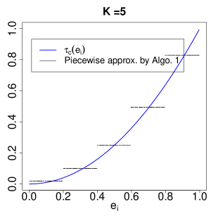
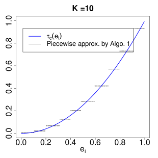
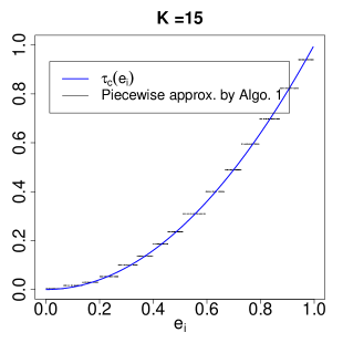
Algorithm 1 transforms arbitrary covariate vector $X_{i}^{*}$ into categorical $\hat{\mathcal{I}}_{i}$ and $\tilde{\mathcal{I}}_{i}$ to fit the interacted 2sls. Note that $\hat{\mathcal{I}}_{i}$ and $\tilde{\mathcal{I}}_{i}$ are discretized approximations to the actual $e_{i}$ . Heuristically, an IV that is conditionally valid given $e_{i}$ can be viewed as “approximately valid” given $\hat{\mathcal{I}}_{i}$ or $\tilde{\mathcal{I}}_{i}$ . This, together with Theorem 1 and Corollary 1, provides the heuristic justification of the resulting $\hat{\tau}_{\times\times}^{*}$ and $\hat{\beta}_{\textsc{2sls}}^{*}$ to approximate the LATE and subgroup LATEs

\displaystyle\tau_{[k]\textup{c}}=\mathbb{E}(\tau_{i}\mid e_{i}\in\mathcal{S}_{k},\,U_{i}=\textup{c}),\quad\text{where}\ \ k=1,\ldots,K,

(15)

respectively. The subgroup LATEs in (15) further provide a piecewise approximation to $\tau_{\textup{c}}(e_{i})$ by assuming $\tau_{\textup{c}}(e_{i})\approx\tau_{[k]\textup{c}}$ for $e_{i}\in\mathcal{S}_{k}$ . This is analogous to the idea of regressogram in nonparametric regression (Liero, 1989; Wasserman, 2006).

6 Simulation

6.1 Interacted 2SLS for estimating LATE

We now use a simulated example to illustrate the advantage of the interacted 2sls for estimating the LATE. Assume the following model for $(X_{i},Z_{i},D_{i},Y_{i})$ :

(i)

$X_{i}=(1,X_{i1})^{\top}$ , where $X_{i1}\sim$ Bernoulli(0.5).
(ii)

$Z_{i}\mid X_{i}\sim$ Bernoulli $(0.5+0.4X_{i1})$ .
(iii)

$D_{i}=1(U_{i}=\textup{a})+Z_{i}\cdot 1(U_{i}=\textup{c})$ , where $\mathbb{P}(U_{i}=\textup{a}\mid X_{i})=0.1$ and $\mathbb{P}(U_{i}=\textup{c}\mid X_{i})=0.7-0.5X_{i1}$ .
(iv)

$Y_{i}=D_{i}Y_{i}(1)+(1-D_{i})Y_{i}(0)$ with $Y_{i}(0)=0$ and $Y_{i}(1)=-1+5X_{i1}$ .

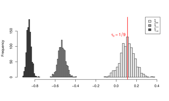
The data-generating process ensures $\tau_{[1]\textup{c}}=\mathbb{E}(\tau_{i}\mid X_{i1}=1,U_{i}=\textup{c})=4$ , $\tau_{[2]\textup{c}}=\mathbb{E}(\tau_{i}\mid X_{i1}=0,U_{i}=\textup{c})=-1$ , and $\tau_{\textup{c}}=1/9$ . For each replication, we generate $N=10000$ independent realizations of $(X_{i},Z_{i},D_{i},Y_{i})$ and compute $\hat{\tau}_{++}$ , $\hat{\tau}_{\times\times}$ , and $\hat{\tau}_{\times+}$ from the additive, interacted, and interacted-additive 2sls in Definitions 1–4; c.f. Table 1. We use the method of moments to estimate the complier average of $X_{i1}$ in computing $\hat{\tau}_{\times\times}$ .

Figure 1 shows the distributions of the three estimators over 1000 replications. Almost all realizations of $\hat{\tau}_{++}$ and $\hat{\tau}_{\times+}$ are below $-0.4$ while the actual $\tau_{\textup{c}}$ is positive. In contrast, the distribution of $\hat{\tau}_{\times\times}$ is approximately centered at the actual $\tau_{\textup{c}}$ , which is coherent with Theorem 1 for categorical covariates.

Refer to caption — Figure 1: Distributions of $\hat{\tau}_{\times\times}$ , $\hat{\tau}_{++}$ , and $\hat{\tau}_{\times+}$ over 1000 replications.

6.2 Approximation of LATE by Algorithm 1.

We now illustrate the improvement of Algorithm 1 for estimating the LATE. Assume the following model for generating $(X_{i},Z_{i},D_{i},Y_{i})$ .

(i)

$X_{i}=(1,X_{i1},X_{i2})^{\top}$ , where $X_{i1}$ and $X_{i2}$ are independent standard normals.
(ii)

$\mathbb{P}(Z_{i}\mid X_{i})=\{1+\exp(X_{i1}+X_{i2})\}^{-1}$ .
(iii)

$D_{i}=Z_{i}\cdot 1(U_{i}=\textup{c})+1(U_{i}=\textup{a})$ , where $\mathbb{P}(U_{i}=\textup{c})=0.7$ and $\mathbb{P}(U_{i}=\textup{a})=0.2$ .
(iv)

$Y_{i}=D_{i}Y_{i}(1)+(1-D_{i})Y_{i}(0)$ with $Y_{i}(0)=0$ and $Y_{i}(1)=X_{1i}^{2}+X_{2i}^{2}$ .

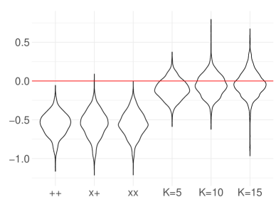
For each replication, we generate $N=1000$ independent realizations of $(X_{i},Z_{i},D_{i},Y_{i})$ and compute $\hat{\tau}_{\times\times}^{*}$ by Algorithm 1. We consider $K=5,10,15$ to evaluate the impact of the number of strata on estimation. For comparison, we also compute $\hat{\tau}_{++}$ , $\hat{\tau}_{\times\times}$ , and $\hat{\tau}_{\times+}$ from the additive, interacted, and interacted-additive 2sls in Definitions 1–4.

Figure 2 shows the violin plot of the deviations of the resulting estimators from the LATE over 1000 replications. The three estimators by Algorithm 1 substantially reduce the biases compared with $\hat{\tau}_{++}$ , $\hat{\tau}_{\times+}$ , and $\hat{\tau}_{\times\times}$ . In addition, increasing the number of strata further reduces the bias but increases variability. Table 2 summarizes the means and standard deviations of the deviations.

Table 2: Biases and standard deviations of the 2sls estimators over 1000 replications.

	$\hat{\tau}_{++}$	$\hat{\tau}_{\times+}$	$\hat{\tau}_{\times\times}$	$\hat{\tau}_{\times\times}^{*}$ from Algorithm 1
	$\hat{\tau}_{++}$	$\hat{\tau}_{\times+}$	$\hat{\tau}_{\times\times}$	$K=5$	$K=10$	$K=15$
Bias	$-0.559$	$-0.556$	$-0.557$	$-0.106$	$-0.054$	$-0.043$
Standard dev.	0.144	0.165	0.157	0.124	0.140	0.336

6.3 Possible inconsistency for estimating $\beta_{\textup{c}}$

We now illustrate the possible inconsistency of the interacted 2sls in Theorem 2. Assume the following model for $(X_{i},Z_{i},D_{i},Y_{i})$ :

(i)

$X_{i}=(1,X_{i1})^{\top}$ , where $X_{i1}\sim$ Uniform(0,1).
(ii)

$Z_{i}\sim$ Bernoulli( $e_{i}$ ) with $e_{i}=X_{i1}$ .
(iii)

$D_{i}=Z_{i}\cdot 1(U_{i}=\textup{c})+1(U_{i}=\textup{a})$ , where $\mathbb{P}(U_{i}=\textup{c})=0.7$ and $\mathbb{P}(U_{i}=\textup{a})=0.2$ .
(iv)

$Y_{i}=D_{i}Y_{i}(1)+(1-D_{i})Y_{i}(0)$ with $Y_{i}(0)=0$ and $Y_{i}(1)=X_{i1}^{2}$ .

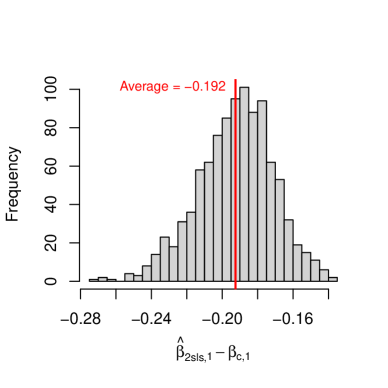
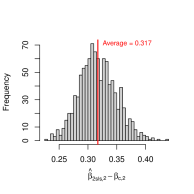
The data-generating process ensures $\tau_{i}=Y_{i}(1)-Y_{i}(0)=X_{i1}^{2}$ and $\beta_{\textup{c}}=(-1/6,1)^{\top}$ .

For each replication, we generate $N=1000$ independent realizations of $(X_{i},Z_{i},D_{i},Y_{i})$ and compute $\hat{\beta}_{\textsc{2sls}}$ from the interacted 2sls in Definition 2. Figure 3 shows the distribution of $\hat{\beta}_{\textsc{2sls}}-\beta_{\textup{c}}$ over 1000 replications, indicating clear empirical biases in both dimensions.

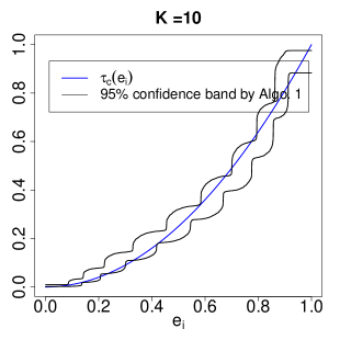
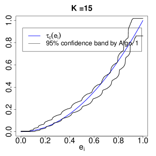
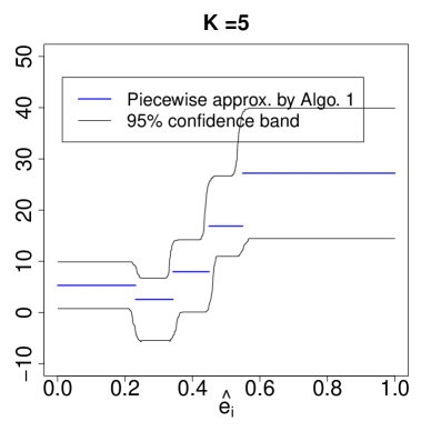
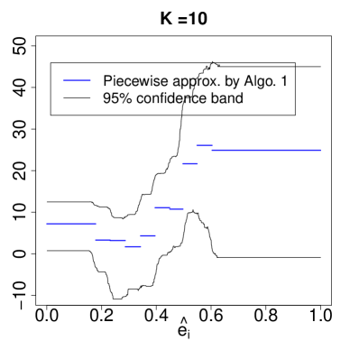
6.4 Approximation of $\tau_{\textup{c}}(e_{i})$ by Algorithm 1.

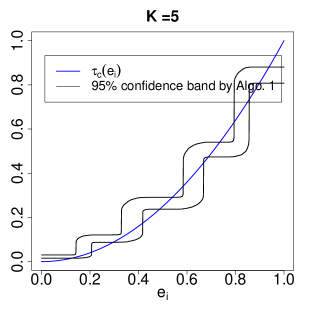
We now illustrate the utility of Algorithm 1 for approximating the conditional LATEs given the IV propensity score. Assume the same model as in Section 6.3 for generating $(X_{i},Z_{i},D_{i},Y_{i})$ . The data-generating process ensures $\tau_{i}=X_{i1}^{2}=e_{i}^{2}$ with $\tau_{\textup{c}}(e_{i})=\mathbb{E}(\tau_{i}\mid e_{i},U_{i}=\textup{c})=e_{i}^{2}$ .

To use Algorithm 1 to approximate $\tau_{\textup{c}}(e_{i})$ , we estimate the IV propensity score by the logistic regression of $Z_{i}$ on $X_{i}$ , and create the strata by dividing $(\hat{e}_{i})_{i=1}^{N}$ into $K$ equal-sized bins. Figure 4 shows the results at $K=5,10,15$ . The first row is based on one replication to illustrate the evolution of the approximation as $K$ increases. The second row shows the 95% confidence bands based on 3000 replications. The coverage of the confidence band improves as $K$ increases. Note that the logistic regression for estimating $e_{i}$ is misspecified in this example. The results suggest the robustness of the method to misspecification of the propensity score model with moderate number of strata.

7 Application

We now apply Algorithm 1 to the dataset that Abadie (2003) used to study the effects of 401(k) retirement programs on savings. The data contain cross-sectional observations of $N=9275$ units on eligibility for and participation in 401(k) plans along with income and demographic information. The outcome of interest is net financial assets. The treatment variable is an indicator of participation in 401(k) plans, and the IV is an indicator of 401(k) eligibility. Based on Abadie (2003), the IV is conditionally valid after controlling for income, age, and marital status.

Table 3 shows the point estimates of the LATE by the additive, interacted, interacted-additive 2sls in Definitions 1–4 and Algorithm 1, along with their respective bootstrap standard deviations. Figure 5 shows the piecewise approximations of $\tau_{\textup{c}}(e_{i})$ based on Algorithm 1 and the 95% confidence bands based on bootstrapping. The result suggests heterogeneity of conditional LATEs across different strata of the propensity score.

Table 3: Point estimates of the LATE and bootstrap standard deviations by the additive, interacted, additive-interacted 2sls and Algorithm 1 over 1000 replications.

	$\hat{\tau}_{++}$	$\hat{\tau}_{\times+}$	$\hat{\tau}_{\times\times}$	$\hat{\tau}_{\times\times}^{*}$ from Algorithm 1
	$\hat{\tau}_{++}$	$\hat{\tau}_{\times+}$	$\hat{\tau}_{\times\times}$	$K=5$	$K=10$	$K=15$	$K=20$
Point estimate	9.658	11.019	9.296	12.760	12.148	12.008	12.066
Standard dev.	2.222	2.520	1.913	2.076	2.079	2.081	2.089

8 Extensions

8.1 Extension to partially interacted 2SLS

Let $X_{i}$ denote the covariate vector that ensures the conditional validity of the IV. The interacted 2sls in Definition 2 includes interactions of $Z_{i}$ and $D_{i}$ with the whole set of $X_{i}$ in accommodating treatment effect heterogeneity. When treatment effect heterogeneity is of interest or suspected for only a subset of $X_{i}$ , denoted by $V_{i}\subset X_{i}$ , an intuitive modification is to interact $Z_{i}$ and $D_{i}$ with only $V_{i}$ in fitting the 2sls, formalized in Definition 5 below. See Resnjanskij et al. (2024) for a recent application. See also Hirano and Imbens (2001) and Hainmueller et al. (2019) for applications of the partially interacted regression in the ordinary least squares setting.

Definition 5 (Partially interacted 2sls).

(i)

First stage: Fit $\texttt{lm}(D_{i}V_{i}\sim Z_{i}V_{i}+X_{i})$ over $i=1,\ldots,N$ . Denote the fitted values by $\widehat{DV_{i}}$ for $1,\ldots,N$ .
(ii)

Second stage: Fit $\texttt{lm}(Y_{i}\sim\widehat{DV_{i}}+X_{i})$ over $i=1,\ldots,N$ . Let $\hat{\beta}_{\textsc{2sls}}^{\prime}$ denote the coefficient vector of $\widehat{DV_{i}}$ .

The partially interacted 2sls in Definition 5 generalizes the interacted 2sls, and reduces to the interacted 2sls when $V_{i}=X_{i}$ . It is the 2sls procedure corresponding to the working model

\displaystyle Y_{i}=D_{i}V_{i}^{\top}\beta_{DV}+X_{i}^{\top}\beta_{X}+\eta_{i},\quad\text{where}\ \ \mathbb{E}(\eta_{i}\mid Z_{i},X_{i})=0,

(16)

with $V_{i}^{\top}\beta_{DV}$ representing the covariate-dependent treatment effect. We establish below the causal interpretation of $\hat{\beta}_{\textsc{2sls}}^{\prime}$ .

Causal estimand.

Analogous to the definition of $\beta_{\textup{c}}$ in Eq. (4), let $\textup{proj}_{U_{i}=\textup{c}}(\tau_{i}\mid V_{i})=V_{i}^{\top}\beta_{\textup{c}}^{\prime}$ denote the linear projection of $\tau_{i}$ on $V_{i}$ among compliers with

\displaystyle\beta_{\textup{c}}^{\prime}=\textup{argmin}_{b\in\mathbb{R}^{Q}}\mathbb{E}\Big{\{}(\tau_{i}-V_{i}^{\top}b)^{2}\mid U_{i}=\textup{c}\Big{\}}.

Parallel to the discussion after Eq. (4), $V_{i}^{\top}\beta_{\textup{c}}^{\prime}$ is also the linear projection of $\tau_{\textup{c}}(X_{i})$ on $V_{i}$ among compliers with $\beta_{\textup{c}}^{\prime}=\textup{argmin}_{b\in\mathbb{R}^{Q}}\mathbb{E}[\{\tau_{\textup{c}}(X_{i})-V_{i}^{\top}b\}^{2}\mid U_{i}=\textup{c}]$ . This ensures $V_{i}^{\top}\beta_{\textup{c}}^{\prime}$ is the best linear approximation to both $\tau_{i}$ and $\tau_{\textup{c}}(X_{i})$ based on $V_{i}$ . We define $\beta_{\textup{c}}^{\prime}$ as the causal estimand for quantifying treatment effect heterogeneity with regard to $V_{i}$ among compliers.

Properties of $\hat{\beta}_{\textsc{2sls}}^{\prime}$ for estimating $\beta_{\textup{c}}^{\prime}$ .

Let $\beta_{\textsc{2sls}}^{\prime}$ denote the probability limit of $\hat{\beta}_{\textsc{2sls}}^{\prime}$ . Proposition 4 below generalizes Theorem 2 and states three sufficient conditions for $\beta_{\textsc{2sls}}^{\prime}$ to identify $\beta_{\textup{c}}^{\prime}$ .

Proposition 4.

Assume $X_{i}=(V_{i}^{\top},W_{i}^{\top})^{\top}\in\mathbb{R}^{K}$ , where $V_{i}\in\mathbb{R}^{Q}$ and $W_{i}\in\mathbb{R}^{K-Q}$ with $Q\leq K$ . Let $\widetilde{DV_{i}}$ denote the residual of the linear projection of $\textup{proj}(D_{i}V_{i}\mid Z_{i}V_{i},X_{i})$ on $X_{i}$ . Let $B^{\prime}=\mathbb{E}\{\widetilde{DV_{i}}\cdot(Y_{i}-D_{i}V_{i}^{\top}\beta_{\textup{c}}^{\prime})\}$ . Assume Assumption 1. Then

\displaystyle\beta_{\textsc{2sls}}^{\prime}=\beta_{\textup{c}}^{\prime}+\{\mathbb{E}(\widetilde{DV_{i}}\cdot\widetilde{DV_{i}}^{\top})\}^{-1}B^{\prime},

where $B^{\prime}=0$ if any of the following conditions holds:

(i)

Categorical covariates: $V_{i}$ is categorical with $Q$ levels, and satisfies $\mathbb{E}(Z_{i}\mid X_{i})=\mathbb{E}(Z_{i}\mid V_{i})$ and $\textup{proj}(Z_{i}V_{i}\mid X_{i})=\textup{proj}(Z_{i}V_{i}\mid V_{i})$ .
(ii)

Random assignment of IV: $Z_{i}\perp\!\!\!\perp X_{i}$ .
(iii)

Correct interacted outcome model: The interacted working model (16) is correct.

Proposition 4(i) parallels the identification of $\beta_{\textup{c}}$ with categorical covariates by Theorem 2, and states a sufficient condition for $\beta_{\textsc{2sls}}^{\prime}$ to identify $\beta_{\textup{c}}^{\prime}$ when $V_{i}$ is categorical. A special case is when $X_{i}$ encodes two categorical variables and $V_{i}$ corresponds to one of them.

Proposition 4(ii) parallels the identification of $\beta_{\textup{c}}$ with randomly assigned IV by Theorem 2, and ensures $\beta_{\textsc{2sls}}^{\prime}=\beta_{\textup{c}}^{\prime}$ when $Z_{i}$ is unconditionally valid.

Proposition 4(iii) parallels the identification of $\beta_{\textup{c}}$ under correct interacted working model (1) by Theorem 2, and ensures $\beta_{\textsc{2sls}}^{\prime}=\beta_{\textup{c}}^{\prime}$ when the working model (16) underlying the partially interacted 2sls is correct.

We relegate possible relaxations of these three sufficient conditions to Lemma S9 in the Supplementary Material.

8.2 Interacted OLS as a special case

Ordinary least squares (ols) is a special case of 2sls with $Z_{i}=D_{i}$ . Therefore, our theory extends to the ols regression of $Y_{i}$ on $(D_{i}X_{i},X_{i})$ when $D_{i}$ is conditionally randomized. Interestingly, the discussion of interacted ols in observational studies is largely missing except Rosenbaum and Rubin (1983). See Aronow and Samii (2016) and Chattopadhyay and Zubizarreta (2023) for the corresponding discussion of additive ols.

Renew $X_{i}^{0}=(1,X_{i1}-\bar{X}_{1},\ldots,X_{i,K-1}-\bar{X}_{K-1})^{\top}$ , where $\bar{X}_{k}=N^{-1}\sum_{i=1}^{N}X_{ik}$ , as a variant of $X_{i}$ centered by covariate means over all units. Let $\hat{\tau}_{\textsc{ols}}$ be the coefficient of $D_{i}$ in $\texttt{lm}(Y_{i}\sim D_{i}X_{i}^{0}+X_{i}^{0})$ , as the ols analog of $\hat{\tau}_{\times\times}$ when $Z_{i}=D_{i}$ . Let $\hat{\beta}_{\textsc{ols}}$ be the coefficient vector of $D_{i}X_{i}$ in $\texttt{lm}(Y_{i}\sim D_{i}X_{i}+X_{i})$ , as the analog of $\hat{\beta}_{\textsc{2sls}}$ when $Z_{i}=D_{i}$ . We derive below the causal interpretation of $\hat{\tau}_{\textsc{ols}}$ and $\hat{\beta}_{\textsc{ols}}$ .

First, letting $Z_{i}=D_{i}$ ensures that all units are compliers. The definitions of $\tau_{\textup{c}}$ and $\beta_{\textup{c}}$ in Eqs. (2) and (4) simplify to $\tau=\mathbb{E}(\tau_{i})$ , as the average treatment effect, and $\beta=\textup{argmin}_{b\in\mathbb{R}^{K}}\mathbb{E}\{(\tau_{i}-X_{i}^{\top}b)^{2}\}$ , as the coefficient vector in the linear projection of $\tau_{i}$ on $X_{i}$ , respectively. The IV assumptions in Assumption 1 simplify to the selection on observables and overlap assumptions on $D_{i}$ , summarized in Assumption 4 below.

Assumption 4.

(i)

Selection on observables: $D_{i}\perp\!\!\!\perp\{Y_{i}(d):d=0,1\}\mid X_{i}$ ;
(ii)

Overlap: $0<\mathbb{P}(D_{i}=1\mid X_{i})<1$ .

Proposition 5 below follows from applying Theorems 1–2 with $Z_{i}=D_{i}$ , and establishes the properties of $\hat{\tau}_{\textsc{ols}}$ and $\hat{\beta}_{\textsc{ols}}$ for estimating $\tau$ and $\beta$ .

Proposition 5.

Let $\tau_{\textsc{ols}}$ and $\beta_{\textsc{ols}}$ denote the probability limits of $\hat{\tau}_{\textsc{ols}}$ and $\hat{\beta}_{\textsc{ols}}$ . Assume Assumption 4. Then $\tau_{\textsc{ols}}=\tau$ and $\beta_{\textsc{ols}}=\beta$ if either of the following conditions holds:

(i)

Linear treatment-covariate interactions: $\mathbb{E}(D_{i}X_{i}\mid X_{i})$ is linear in $X_{i}$ .
(ii)

Linear outcome: $Y_{i}=D_{i}X_{i}^{\top}\beta_{ZX}+X_{i}^{\top}\beta_{X}+\eta_{i}$ , where $\mathbb{E}(\eta_{i}\mid D_{i},X_{i})=0$ , for some fixed $\beta_{ZX},\beta_{X}\in\mathbb{R}^{K}$ .

Parallel to Proposition 1(i), Proposition 5(i) encompasses (a) categorical covariates and (b) randomly assigned treatment as special cases. Proposition 5(ii) implies that the interacted regression is correctly specified.

Similar results can be obtained for partially interacted ols regression of $Y_{i}$ on $(D_{i}V_{i},X_{i})$ by letting $Z_{i}=D_{i}$ in Proposition 4. We omit the details.

9 Discussion

We formalized the interacted 2sls as an intuitive approach for incorporate treatment effect heterogeneity in IV analyses, and established its properties for estimating the LATE and systematic treatment effect variation under the LATE framework. We showed that the coefficients from the interacted 2sls are consistent for estimating the LATE and treatment effect heterogeneity with regard to covariates among compliers if either (i) the IV-covariate interactions are linear in the covariates or (ii) the linear outcome model underlying the interacted 2sls is correct. Condition (i) includes categorical covariates and randomly assigned IV as special cases. When neither condition (i) nor condition (ii) holds, we propose a stratification strategy based on the IV propensity score to approximate the LATE and treatment effect heterogeneity with regard to the IV propensity score. We leave possible relaxations of the identifying conditions for the LATE to future work.

S1 Additional results

Population 2SLS estimand.

Linear projection gives the population analog of least-squares regression. Proposition S1 below formalizes the population analog of the interacted 2sls in Definition 2.

Proposition S1.

Define the population interacted 2sls as the combination of the following two linear projections:

(i)

First stage: the linear projection of $D_{i}X_{i}$ on $(Z_{i}X_{i}^{\top},X_{i}^{\top})^{\top}$ , denoted by $\textup{proj}(D_{i}X_{i}\mid Z_{i}X_{i},X_{i})$ .
(ii)

Second stage: the linear projection of $Y_{i}$ on the concatenation of $\textup{proj}(D_{i}X_{i}\mid Z_{i}X_{i},X_{i})$ and $X_{i}$ .

Then $\beta_{\textsc{2sls}}$ equals the coefficient vector of $\textup{proj}(D_{i}X_{i}\mid Z_{i}X_{i},X_{i})$ from the second stage.

Invariance of the interacted 2SLS to nondegenerate linear transformations.

The values of $\hat{\beta}_{\textsc{2sls}}$ from the interacted 2sls and $\beta_{\textup{c}}$ from Eq. (4) both depend on the choice of the covariate vector $X_{i}$ . Let $\hat{\beta}_{\textsc{2sls}}(X_{i})$ , $\beta_{\textsc{2sls}}(X_{i})$ , and $\beta_{\textup{c}}(X_{i})$ denote the values of $\hat{\beta}_{\textsc{2sls}}$ , $\beta_{\textsc{2sls}}$ , and $\beta_{\textup{c}}$ corresponding to covariate vector $X_{i}$ . Proposition S2 below states their invariance to nondegenerate linear transformation of $X_{i}$ .

Proposition S2.

For $K\times 1$ covariate vectors $\{X_{i}\in\mathbb{R}^{K}:i=1,\ldots,N\}$ and an invertible $K\times K$ matrix $\Gamma$ , we have

\displaystyle\hat{\beta}_{\textsc{2sls}}(\Gamma X_{i})=(\Gamma^{\top})^{-1}\hat{\beta}_{\textsc{2sls}}(X_{i}),\quad\beta_{\textsc{2sls}}(\Gamma X_{i})=(\Gamma^{\top})^{-1}\beta_{\textsc{2sls}}(X_{i}),\quad\beta_{\textup{c}}(\Gamma X_{i})=(\Gamma^{\top})^{-1}\beta_{\textup{c}}(X_{i}).

Generalized additive 2SLS.

Definition S1 below generalizes the additive and interacted-additive 2sls in Definitions 1 and 4 to arbitrary first stage.

Definition S1 (Generalized additive 2sls).

Let $R_{i}=R(X_{i},Z_{i})$ be an arbitrary vector function of $(X_{i},Z_{i})$ .

(i)

First stage: Fit $\texttt{lm}(D_{i}\sim R_{i})$ over $i=1,\ldots,N$ . Denote the fitted values by $\hat{D}_{i}$ for $i=1,\ldots,N$ .
(ii)

Second stage: Fit $\texttt{lm}(Y_{i}\sim\hat{D}_{i}+X_{i})$ over $i=1,\ldots,N$ . Denote the coefficient of $\hat{D}_{i}$ by $\hat{\tau}_{*+}$ .

We use the subscript $*+$ to represent the arbitrary first stage and additive second stage. The additive 2sls in Definition 1 is a special case of the generalized additive 2sls with $R_{i}=(Z_{i},X_{i}^{\top})^{\top}$ . The interacted-additive 2sls in Definition 4 is a special case with $R_{i}=(Z_{i}X_{i}^{\top},X_{i}^{\top})^{\top}$ .

Let $\tau_{*+}$ denote the probability limit of $\hat{\tau}_{*+}$ . Proposition S3 below clarifies the causal interpretation of $\tau_{*+}$ .

Let $\check{D}_{i}=\textup{proj}(D_{i}\mid R_{i})$ denote the population fitted value from the first stage of the generalized additive 2sls. Let $\tilde{D}_{i}=\textup{res}(\check{D}_{i}\mid X_{i})$ . Let $\Delta_{i}=Y_{i}(0)$ for compliers and never-takers and $\Delta_{i}=Y_{i}(1)-\tau_{\textup{c}}(X_{i})$ for always-takers. Recall

\displaystyle w(X_{i})=\dfrac{\operatorname{var}\{\mathbb{E}(D_{i}\mid Z_{i},X_{i})\mid X_{i}\}}{\mathbb{E}\big{[}\operatorname{var}\{\mathbb{E}(D_{i}\mid Z_{i},X_{i})\mid X_{i}\}\big{]}}.

Proposition S3.

Assume Assumption 1. Then $\tau_{*+}=\mathbb{E}\left\{\alpha(X_{i})\cdot\tau_{\textup{c}}(X_{i})\right\}+\{\mathbb{E}(\tilde{D}_{i}^{2})\}^{-1}B$ , where

\displaystyle\alpha(X_{i})=\dfrac{\mathbb{E}(D_{i}\tilde{D}_{i}\mid X_{i})}{\mathbb{E}(\tilde{D}_{i}^{2})},\quad B=\mathbb{E}\Big{[}\Big{\{}\mathbb{E}(\check{D}_{i}\mid X_{i})-\textup{proj}(\check{D}_{i}\mid X_{i})\Big{\}}\cdot\Big{\{}\mathbb{E}(\Delta_{i}\mid X_{i})-\textup{proj}(\Delta_{i}\mid X_{i})\Big{\}}\Big{]}.

In particular,

(i)
$B=0$ if either of the following conditions holds:
1. (a)
  
  $\mathbb{E}(\check{D}_{i}\mid X_{i})$ is linear in $X_{i}$ .
2. (b)
  
  $\mathbb{E}(\Delta\mid X_{i})$ is linear in $X_{i}$ .
(ii)
$\alpha(X_{i})=w(X_{i})$ if both of the following conditions hold:
1. (a)
  
  $\mathbb{E}(\check{D}_{i}\mid X_{i})$ is linear in $X_{i}$ .
2. (b)
  
  $\check{D}_{i}=\mathbb{E}(D_{i}\mid Z_{i},X_{i})$ ; i.e., the arbitrary first stage is correct.

S2 Lemmas

S2.1 Projection and conditional expectation

Lemmas S1–S3 below review some standard results regarding projection and conditional expectation. We omit the proofs.

Lemma S1.

For random vectors $A$ and $B$ ,

(i)

$\mathbb{E}(A\mid B)=\textup{proj}(A\mid B)$ if and only if $\mathbb{E}(A\mid B)$ is linear in $B$ ;
(ii)

if $A\perp\!\!\!\perp B$ , then $\mathbb{E}(AB\mid B)=\textup{proj}(AB\mid B)=\mathbb{E}(A)B$ ;
(iii)

if $A$ is binary, then $\mathbb{E}(A\mid B)$ is constant implies $A\perp\!\!\!\perp B$ .

Lemma S2.

Let $X$ be an $m\times 1$ random vector with $\mathbb{E}(XX^{\top})$ being invertible. Then

(i)

for any subvector of $X$ , denoted by $V$ , $\mathbb{E}(VV^{\top})$ is invertible.
(ii)

$X$ takes at least $m$ distinct values.
(iii)

If $X$ takes exactly $m$ distinct values, denoted by $x_{1},\ldots,x_{m}\in\mathbb{R}^{m}$ , then
-

$\Gamma=(x_{1},\ldots,x_{m})\in\mathbb{R}^{m\times m}$ is invertible, and $X=\Gamma(1(X=x_{1}),\ldots,1(X=x_{m}))^{\top}$ .
-

$XX^{\top}$ is component-wise linear in $X$ .
-

for any random vector $A$ , $\mathbb{E}(A\mid X)$ is linear in $X$ .

Lemma S3 (Population Frisch–Waugh–Lovell (FWL)).

For a random variable $Y$ , a $p_{1}\times 1$ random vector $X_{1}$ , and a $p_{2}\times 1$ random vector $X_{2}$ , let $\tilde{Y}=\textup{res}(Y\mid X_{2})$ and $\tilde{X}_{1}=\textup{res}(X_{1}\mid X_{2})$ denote the residuals from the linear projections of $Y$ and $X_{1}$ on $X_{2}$ , respectively. Then the coefficient vector of $X_{1}$ in the linear projection of $Y$ on $(X_{1}^{\top},X_{2}^{\top})^{\top}$ equals the coefficient vector of $\tilde{X}_{1}$ in the linear projection of $Y$ or $\tilde{Y}$ on $\tilde{X}_{1}$ .

S2.2 Lemmas for the interacted 2SLS

Assumption S1 below states the rank condition for the interacted 2sls, which we assume implicitly throughout the main paper. By the law of large numbers,

\displaystyle\beta_{\textsc{2sls}}=\text{the first $K$ dimensions of $\left[\mathbb{E}\left\{\begin{pmatrix}Z_{i}X_{i}\\ X_{i}\end{pmatrix}\Big{(}D_{i}X_{i}^{\top},X_{i}^{\top}\Big{)}\right\}\right]^{-1}\mathbb{E}\left\{\begin{pmatrix}Z_{i}X_{i}\\ X_{i}\end{pmatrix}Y_{i}\right\}$}.

Assumption S1.

$\mathbb{E}\left\{\begin{pmatrix}Z_{i}X_{i}\\ X_{i}\end{pmatrix}\Big{(}D_{i}X_{i}^{\top},X_{i}^{\top}\Big{)}\right\}$ is invertible.

Lemma S4 below states some implications of Assumption S1 that are useful for the proofs.

Lemma S4.

Recall $C_{0},C_{1},C_{2}$ from (S1). Assume Assumption S1. We have

(i)

$\mathbb{E}\left\{\begin{pmatrix}Z_{i}X_{i}\\ X_{i}\end{pmatrix}\Big{(}Z_{i}X_{i}^{\top},X_{i}^{\top}\Big{)}\right\}$ and $\mathbb{E}(X_{i}X^{\top}_{i})$ are both invertible with

	$\displaystyle(C_{1},C_{0})$	$\displaystyle=$	$\displaystyle\mathbb{E}\Big{\{}D_{i}X_{i}(Z_{i}X_{i}^{\top},X^{\top}_{i})\Big{\}}\left[\mathbb{E}\left\{\begin{pmatrix}Z_{i}X_{i}\\ X_{i}\end{pmatrix}(Z_{i}X_{i}^{\top},X^{\top}_{i})\right\}\right]^{-1},$
	$\displaystyle C_{2}$	$\displaystyle=$	$\displaystyle\mathbb{E}(Z_{i}X_{i}X^{\top}_{i})\big{\{}\mathbb{E}(X_{i}X^{\top}_{i})\big{\}}^{-1}.$

(ii)

$X_{i}$ takes at least $K$ distinct values.
(iii)

$C_{1}$ , $C_{2}$ , and $I_{K}-C_{2}$ are all invertible.

Proof of Lemma S4.

We verify below Lemma S4(i)–(iii), respectively. We omit the subscript $i$ in the proof. Let

\displaystyle\Gamma_{1}=\mathbb{E}\left\{\begin{pmatrix}DX\\ X\end{pmatrix}(ZX^{\top},X^{\top})\right\},\quad\Gamma_{2}=\mathbb{E}\left\{\begin{pmatrix}ZX\\ X\end{pmatrix}\Big{(}ZX^{\top},X^{\top}\Big{)}\right\}

be shorthand notation with $\Gamma_{1}$ being invertible under Assumption S1.

Proof of Lemma S4(i):

We prove the result by contradiction. Note that $\Gamma_{2}$ is positive semidefinite. If $\Gamma_{2}$ is degenerate, then there exists a nonzero vector $a$ such that $a^{\top}\Gamma_{2}a=0$ . This implies

\displaystyle 0=a^{\top}\mathbb{E}\left\{\begin{pmatrix}ZX\\ X\end{pmatrix}(ZX^{\top},X^{\top})\right\}a=\mathbb{E}\left\{a^{\top}\begin{pmatrix}ZX\\ X\end{pmatrix}(ZX^{\top},X^{\top})a\right\}

such that $(ZX^{\top},X^{\top})a=0$ . As a result, we have

\Gamma_{1}a=\mathbb{E}\left\{\begin{pmatrix}DX\\ X\end{pmatrix}(ZX^{\top},X^{\top})\right\}a=\mathbb{E}\left\{\begin{pmatrix}DX\\ X\end{pmatrix}(ZX^{\top},X^{\top})a\right\}=0

for a nonzero $a$ . This contradicts with $\Gamma_{1}$ being invertible.

That $\mathbb{E}(XX^{\top})$ is invertible then follows from Lemma S2(i).

Proof of Lemma S4(ii).

Given $\mathbb{E}(XX^{\top})$ is invertible as we just proved, the result follows from Lemma S2(ii).

Proof of Lemma S4(iii):

Properties of linear projection ensure

\displaystyle\textup{proj}\left\{\begin{pmatrix}DX\\ X\end{pmatrix}\mid ZX,X\right\}=\begin{pmatrix}C_{1}&C_{0}\\ 0&I_{K}\end{pmatrix}\begin{pmatrix}ZX\\ X\end{pmatrix},

with

\displaystyle\begin{pmatrix}C_{1}&C_{0}\\ 0&I_{K}\end{pmatrix}=\mathbb{E}\left\{\begin{pmatrix}DX\\ X\end{pmatrix}(ZX^{\top},X^{\top})\right\}\left[\mathbb{E}\left\{\begin{pmatrix}ZX\\ X\end{pmatrix}(ZX^{\top},X^{\top})\right\}\right]^{-1}=\Gamma_{1}\Gamma_{2}^{-1}.

(S8)

This ensures $\det(C_{1})=\det\begin{pmatrix}C_{1}&C_{0}\\ 0&I_{K}\end{pmatrix}=\det(\Gamma_{1}\Gamma_{2}^{-1})\neq 0$ .

In addition, note that

	$\displaystyle I_{K}-C_{2}$	$\displaystyle=$	$\displaystyle\mathbb{E}(XX^{\top})\cdot\left\{\mathbb{E}(XX^{\top})\right\}^{-1}-\mathbb{E}(ZXX^{\top})\cdot\left\{\mathbb{E}(XX^{\top})\right\}^{-1}$
		$\displaystyle=$	$\displaystyle\mathbb{E}\left\{(1-Z)XX^{\top}\right\}\cdot\left\{\mathbb{E}(XX^{\top})\right\}^{-1}.$

To show that $C_{2}$ and $I_{K}-C_{2}$ are invertible, it suffices to show that $\mathbb{E}(ZXX^{\top})$ and $\mathbb{E}\{(1-Z)XX^{\top}\}$ are invertible. This is ensured by

$\displaystyle 0<\det(\Gamma_{2})$	$\displaystyle=$	$\displaystyle\det\left\{\begin{pmatrix}\mathbb{E}(ZXX^{\top})&\mathbb{E}(ZXX^{\top})\\ \mathbb{E}(ZXX^{\top})&\mathbb{E}(XX^{\top})\end{pmatrix}\right\}$
	$\displaystyle=$	$\displaystyle\det\left\{\begin{pmatrix}\mathbb{E}(ZXX^{\top})&\mathbb{E}(ZXX^{\top})\\ 0&\mathbb{E}\left\{(1-Z)XX^{\top}\right\}\end{pmatrix}\right\}$
	$\displaystyle=$	$\displaystyle\det\Big{\{}\mathbb{E}(ZXX^{\top})\Big{\}}\cdot\det\Big{[}\mathbb{E}\left\{(1-Z)XX^{\top}\right\}\Big{]}.$

∎

Lemma S5 below formalizes the sufficiency and necessity of Assumption 3 to ensure the combination of conditions (11) and (13); c.f. Section 4.2.

Lemma S5.

Assume Assumption 1. Assumption 3 is both sufficient and necessary for

\displaystyle\mathbb{E}(\Delta_{i}\mid X_{i})=X_{i}^{\top}\beta_{\Delta}\ \ \text{for some $\beta_{\Delta}\in\mathbb{R}^{K}$},\quad\tau_{\textup{c}}(X_{i})=\mathbb{E}(\tau_{i}\mid X_{i},U_{i}=\textup{c})=X_{i}^{\top}\beta_{\textup{c}}.

(S9)

Proof of Lemma S5.

We verify below the sufficiency and necessity of Assumption 3, respectively.

Sufficiency.

Under Assumption 3, we have

\displaystyle\begin{array}[]{rcl }\eta_{i}&=&Y_{i}-D_{i}X_{i}^{\top}\beta_{DX}-X_{i}^{\top}\beta_{X}\\ &=&\left\{\begin{array}[]{lll}Y_{i}(1)-X_{i}^{\top}(\beta_{DX}+\beta_{X})&\text{if $U_{i}=\textup{a}$}\\ Y_{i}(0)-X_{i}^{\top}\beta_{X}&\text{if $U_{i}=\textup{n}$}\\ Y_{i}(0)-X_{i}^{\top}\beta_{X}+Z_{i}(\tau_{i}-X_{i}^{\top}\beta_{DX})&\text{if $U_{i}=\textup{c}$}\end{array}\right.\\ &=&\lambda_{i}+Z_{i}\zeta_{i},\end{array}

(S16)

where

\displaystyle\lambda_{i}=\left\{\begin{array}[]{lll}Y_{i}(1)-X_{i}^{\top}(\beta_{DX}+\beta_{X})&\text{if $U_{i}=\textup{a}$}\\ Y_{i}(0)-X_{i}^{\top}\beta_{X}&\text{if $U_{i}=\textup{n}$}\\ Y_{i}(0)-X_{i}^{\top}\beta_{X}&\text{if $U_{i}=\textup{c}$}\end{array}\right.,\quad\zeta_{i}=\left\{\begin{array}[]{cl}\tau_{i}-X_{i}^{\top}\beta_{DX}&\text{if $U_{i}=\textup{c}$}\\ 0&\text{if $U_{i}\neq\textup{c}$}\end{array}\right..

The definition of $\zeta_{i}$ ensures

$\displaystyle\mathbb{E}(\zeta_{i}\mid X_{i})$	$\displaystyle=$	$\displaystyle\mathbb{E}(\zeta_{i}\mid X_{i},U_{i}=\textup{c})\cdot\mathbb{P}(U_{i}=\textup{c}\mid X_{i})$	(S18)
	$\displaystyle=$	$\displaystyle\Big{\{}\mathbb{E}(\tau_{i}\mid X_{i},U_{i}=\textup{c})-X_{i}^{\top}\beta_{DX}\Big{\}}\cdot\mathbb{P}(U_{i}=\textup{c}\mid X_{i})$
	$\displaystyle=$	$\displaystyle\Big{\{}\tau_{\textup{c}}(X_{i})-X_{i}^{\top}\beta_{DX}\Big{\}}\cdot\mathbb{P}(U_{i}=\textup{c}\mid X_{i}).$

This, together with (S16), ensures

$\displaystyle\mathbb{E}(\eta_{i}\mid X_{i},Z_{i})$	$\displaystyle\overset{\eqref{eq:eta_2}}{=}$	$\displaystyle\mathbb{E}(\lambda_{i}\mid X_{i},Z_{i})+Z_{i}\cdot\mathbb{E}(\zeta_{i}\mid X_{i},Z_{i})$	(S19)
	$\displaystyle\overset{\text{Assm. \ref{assm:iv}}}{=}$	$\displaystyle\mathbb{E}(\lambda_{i}\mid X_{i})+Z_{i}\cdot\mathbb{E}(\zeta_{i}\mid X_{i})$
	$\displaystyle\overset{\eqref{eq:zeta}}{=}$	$\displaystyle\mathbb{E}(\lambda_{i}\mid X_{i})+Z_{i}\cdot\Big{\{}\tau_{\textup{c}}(X_{i})-X_{i}^{\top}\beta_{DX}\Big{\}}\cdot\mathbb{P}(U_{i}=\textup{c}\mid X_{i}).$

Under Assumption 3, we have $\mathbb{E}(\eta_{i}\mid X_{i},Z_{i})=0$ so that (S19) implies

	$\displaystyle\mathbb{E}(\lambda_{i}\mid X_{i})$	$\displaystyle\overset{\eqref{eq:eta_3}}{=}$	$\displaystyle\mathbb{E}(\eta_{i}\mid X_{i},Z_{i}=0)\overset{\text{Assm. \ref{assm:linear outcome}}}{=}0,$		(S20)
	$\displaystyle\tau_{\textup{c}}(X_{i})-X_{i}^{\top}\beta_{DX}$	$\displaystyle\overset{\eqref{eq:eta_3}}{=}$	$\displaystyle\dfrac{\mathbb{E}(\eta_{i}\mid X_{i},Z_{i}=1)-\mathbb{E}(\eta_{i}\mid X_{i},Z_{i}=0)}{\mathbb{P}(U_{i}=\textup{c}\mid X_{i})}\overset{\text{Assm. \ref{assm:linear outcome}}}{=}0.$		(S21)

(S21), together with Lemma S1(i), ensures

\displaystyle\tau_{\textup{c}}(X_{i})=X_{i}^{\top}\beta_{DX}\ \ \text{with}\ \ \beta_{\textup{c}}=\beta_{DX}.

(S22)

Plugging (S22) in the definition of $\lambda_{i}$ ensures $\Delta_{i}=\lambda_{i}+X_{i}^{\top}\beta_{X}$ with

\displaystyle\mathbb{E}(\Delta_{i}\mid X_{i})=\mathbb{E}(\lambda_{i}\mid X_{i})+X_{i}^{\top}\beta_{X}\overset{\eqref{eq:lmd_2}}{=}X_{i}^{\top}\beta_{X}.

This, together with (S21), verifies the sufficiency of Assumption 3 to ensure (S9).

Necessity.

We show below that (S9) implies Assumption 3. Recall from (S7) that $Y_{i}-D_{i}X_{i}^{\top}\beta_{\textup{c}}=\Delta_{i}+Z_{i}\epsilon_{i}$ . When (S9) holds, we have $\mathbb{E}(\epsilon_{i}\mid X_{i},U_{i}=\textup{c})=0$ so that

\displaystyle\mathbb{E}(\epsilon_{i}\mid X_{i})=\mathbb{E}(\epsilon_{i}\mid X_{i},U_{i}=\textup{c})\cdot\mathbb{P}(U_{i}=\textup{c}\mid X_{i})=0.

(S23)

This ensures

$\displaystyle\mathbb{E}(Y_{i}-D_{i}X_{i}^{\top}\beta_{\textup{c}}\mid X_{i},Z_{i})$	$\displaystyle\overset{\eqref{eq:Delta_ep}}{=}$	$\displaystyle\mathbb{E}(\Delta_{i}\mid X_{i},Z_{i})+Z_{i}\cdot\mathbb{E}(\epsilon_{i}\mid X_{i},Z_{i})$	(S24)
	$\displaystyle\overset{\text{Assm. \ref{assm:iv}}}{=}$	$\displaystyle\mathbb{E}(\Delta_{i}\mid X_{i})+Z_{i}\cdot\mathbb{E}(\epsilon_{i}\mid X_{i})$
	$\displaystyle\overset{\eqref{eq:cond_linear Delta_tcx}+\eqref{eq:thm2_cond3_necessary_1}}{=}$	$\displaystyle X_{i}^{\top}\beta_{\Delta}.$

Let $\eta^{\prime}_{i}=Y_{i}-D_{i}X_{i}^{\top}\beta_{\textup{c}}-X_{i}^{\top}\beta_{\Delta}$ . We have

	$\displaystyle Y_{i}$	$\displaystyle=$	$\displaystyle D_{i}X_{i}^{\top}\beta_{\textup{c}}+X_{i}^{\top}\beta_{\Delta}+\eta^{\prime}_{i},$
	$\displaystyle\mathbb{E}(\eta^{\prime}_{i}\mid X_{i},Z_{i})$	$\displaystyle=$	$\displaystyle\mathbb{E}(Y_{i}-D_{i}X_{i}^{\top}\beta_{\textup{c}}\mid X_{i},Z_{i})-X_{i}^{\top}\beta_{\Delta}\overset{\eqref{eq:thm2_cond3_necessary}}{=}0$

so that Assumption 3 holds. ∎

Lemma S6 below states a numeric result that we use to prove Corollary 1.

Lemma S6.

Let $\widehat{DX}_{i}$ and $\hat{D}_{i}$ denote the fitted values from $\texttt{lm}(D_{i}X_{i}\sim Z_{i}X_{i}+X_{i})$ and

\displaystyle\texttt{lm}(D_{i}\sim Z_{i}X_{i}+X_{i}),

(S25)

respectively. Assume that $X_{i}$ is categorical with $K$ levels. Then $\widehat{DX}_{i}=\hat{D}_{i}X_{i}$ .

Proof of Lemma S6.

We verify below the result for $X_{i}=(1(X_{i}^{*}=1),\ldots,1(X_{i}^{*}=K))^{\top}$ , where $X_{i}^{*}\in\{1,\ldots,K\}$ denotes a $K$ -level categorical variable. The result for general categorical $X_{i}$ then follows from the invariance of least squares to nondegenerate linear transformations of the regressor vector.

Given $X_{i}=(1(X_{i}^{*}=1),\ldots,1(X_{i}^{*}=K))^{\top}$ , for $k=1,\ldots,K$ , the $k$ th element of $\hat{D}_{i}X_{i}$ equals $\hat{D}_{i}\cdot 1(X_{i}^{*}=k)$ , and the $k$ th element of $\widehat{DX}_{i}$ equals the fitted value from

\displaystyle\texttt{lm}\Big{\{}D_{i}\cdot 1(X_{i}^{*}=k)\sim Z_{i}X_{i}+X_{i}\Big{\}},

(S26)

denoted by $\widehat{DX}_{i}[k]$ . By symmetry, to show that $\widehat{DX}_{i}=\hat{D}_{i}X_{i}$ , it suffices to show that the first element of $\hat{D}_{i}X_{i}$ equals the first element of $\widehat{DX}_{i}$ , i.e.,

\displaystyle\hat{D}_{i}\cdot 1(X_{i}^{*}=1)=\widehat{DX}_{i}[1].

(S27)

We verify (S27) below.

Left-hand side of (S27).

Standard results ensure that (S25) is equivalent to $K$ stratum-wise regressions

\displaystyle\texttt{lm}(D_{i}\sim Z_{i}+1)\quad\text{over units with $X_{i}^{*}=k$}

for $k=1,\ldots,K$ , such that $\hat{D}_{i}$ equals the sample mean of $\{D_{i}:X_{i}^{*}=k,Z_{i}=z\}$ for units with $\{X_{i}^{*}=k,Z_{i}=z\}$ . This ensures

\displaystyle\hat{D}_{i}\cdot 1(X_{i}^{*}=1)=\left\{\begin{array}[]{cll}0&\text{for}&\{i:X_{i}^{*}\neq 1\};\\ \text{sample mean of $\{D_{i}:X_{i}^{*}=1,Z_{i}=z\}$}&\text{for}&\{i:X_{i}^{*}=1;\,Z_{i}=z\}.\end{array}\right.

(S30)

Right-hand side of (S27).

From (S26), $\widehat{DX}_{i}[1]$ equals the fitted value from

\displaystyle\texttt{lm}\Big{\{}D_{i}\cdot 1(X_{i}^{*}=1)\sim Z_{i}X_{i}+X_{i}\Big{\}},

which is equivalent to $K$ stratum-wise regressions

\texttt{lm}\Big{\{}D_{i}\cdot 1(X_{i}^{*}=1)\sim Z_{i}+1\Big{\}}\quad\text{over units with $X_{i}^{*}=k$}

for $k=1,\ldots,K$ . This ensures that $\widehat{DX}_{i}[1]$ equals the sample mean of $\{D_{i}\cdot 1(X_{i}^{*}=1):X_{i}^{*}=k,Z_{i}=z\}$ for units with $\{X_{i}^{*}=k,Z_{i}=z\}$ , which simplies to the follows:

\displaystyle\widehat{DX}_{i}[1]=\left\{\begin{array}[]{cll}0&\text{for}&\{i:X_{i}^{*}\neq 1\};\\ \text{sample mean of $\{D_{i}:X_{i}^{*}=1,Z_{i}=z\}$}&\text{for}&\{i:X_{i}^{*}=1;\,Z_{i}=z\}.\end{array}\right.

This is identical to the expression of $\hat{D}_{i}\cdot 1(X_{i}^{*}=1)$ in (S30), and ensures (S27). ∎

S2.3 Lemmas for the partially interacted 2SLS

Assumption S2 below states the rank condition for the partially interacted 2sls.

Assumption S2.

$\mathbb{E}\left\{\begin{pmatrix}Z_{i}V_{i}\\ X_{i}\end{pmatrix}\Big{(}D_{i}V_{i}^{\top},X_{i}^{\top}\Big{)}\right\}$ is invertible.

Lemma S7 below generalizes Lemma S4 and states some implications of Assumption S2 useful for the proofs. The proof is similar to that of Lemma S4, hence omitted.

Lemma S7.

Assume Assumption S2. We have

(i)

$\mathbb{E}\left\{\begin{pmatrix}Z_{i}V_{i}\\ X_{i}\end{pmatrix}\Big{(}Z_{i}V_{i}^{\top},X_{i}^{\top}\Big{)}\right\}$ , $\mathbb{E}(X_{i}X_{i}^{\top})$ , and $\mathbb{E}(V_{i}V_{i}^{\top})$ are all invertible with

\displaystyle\textup{proj}(D_{i}V_{i}\mid Z_{i}V_{i},X_{i})=C_{1}Z_{i}V_{i}+C_{0}X_{i},\qquad\textup{proj}(Z_{i}V_{i}\mid V_{i})=C_{2}V_{i}

with

	$\displaystyle(C_{1},C_{0})$	$\displaystyle=$	$\displaystyle\mathbb{E}\Big{\{}D_{i}V_{i}(Z_{i}V_{i}^{\top},X_{i}^{\top})\Big{\}}\left[\mathbb{E}\left\{\begin{pmatrix}Z_{i}V_{i}\\ X_{i}\end{pmatrix}\Big{(}Z_{i}V_{i}^{\top},X_{i}^{\top}\Big{)}\right\}\right]^{-1},$
	$\displaystyle C_{2}$	$\displaystyle=$	$\displaystyle\mathbb{E}(Z_{i}V_{i}V_{i}^{\top})\big{\{}\mathbb{E}(V_{i}V_{i}^{\top})\big{\}}^{-1}.$

(ii)

$X_{i}$ takes at least $K$ distinct values. $V_{i}$ takes at least $Q$ distinct values.
(iii)

$C_{1}$ , $C_{2}$ , and $I_{Q}-C_{2}$ are all invertible.

Lemma S8.

Assume $X_{i}=(V_{i}^{\top},W_{i}^{\top})^{\top}\in\mathbb{R}^{K}$ , where $V_{i}\in\mathbb{R}^{Q}$ with $Q\leq K$ and $\mathbb{E}(X_{i}X_{i}^{\top})$ is invertible. Then $\mathbb{E}(Z_{i}V_{i}\mid X_{i})$ is linear in $X_{i}$ and $\mathbb{E}(Z_{i}\mid X_{i})\cdot\{V_{i}-\textup{proj}(Z_{i}V_{i}\mid X_{i})\}$ is linear in $V_{i}$ if any of the following conditions holds:

(i)

$V_{i}$ is categorical with $Q$ levels; $\textup{proj}(Z_{i}V_{i}\mid X_{i})=\textup{proj}(Z_{i}V_{i}\mid V_{i})$ and $\mathbb{E}(Z_{i}\mid X_{i})=\mathbb{E}(Z_{i}\mid V_{i})$ .
(ii)

$Z_{i}\perp\!\!\!\perp X_{i}$ .

Proof of Lemma S8.

To ensure $\mathbb{E}(Z_{i}V_{i}\mid X_{i})$ is linear in $X_{i}$ ,

•

the sufficiency of Lemma S8(i) follows from $\mathbb{E}(Z_{i}V_{i}\mid X_{i})=\mathbb{E}(Z_{i}V_{i}\mid V_{i})$ , where $\mathbb{E}(Z_{i}V_{i}\mid V_{i})$ is linear in $V_{i}$ by Lemma S2(iii).
•

the sufficiency of Lemma S8(ii) follows from $\mathbb{E}(Z_{i}V_{i}\mid X_{i})=\mathbb{E}(Z_{i}\mid X_{i})\cdot V_{i}=\mathbb{E}(Z_{i})\cdot V_{i}$ .

We verify below the sufficiency of the conditions for ensuring that $\mathbb{E}(Z_{i}\mid X_{i})\cdot\{V_{i}-\textup{proj}(Z_{i}V_{i}\mid X_{i})\}$ is linear in $V_{i}$ . We omit the subscript $i$ in the proof.

Proof of Condition (i).

Given $\mathbb{E}(XX^{\top})$ is invertible, Lemma S2(i) ensures that $\mathbb{E}(VV^{\top})$ is invertible. When $V$ is categorical with $Q$ levels, Lemma S2(iii) ensures that $VV^{\top}$ is component-wise linear in $V$ and that $\mathbb{E}(Z\mid V)$ is linear in $V$ . We can write

\displaystyle V-\textup{proj}(ZV\mid V)=CV,\quad\mathbb{E}(Z\mid V)=V^{\top}c,

(S32)

for $C=I_{Q}-\mathbb{E}(ZVV^{\top})\{\mathbb{E}(VV^{\top})\}^{-1}$ and some constant $c\in\mathbb{R}^{Q}$ . This, together with $\textup{proj}(ZV\mid X)=\textup{proj}(ZV\mid V)$ and $\mathbb{E}(Z\mid X)=\mathbb{E}(Z\mid V)$ , ensures

\displaystyle\Big{\{}V-\textup{proj}(ZV\mid X)\Big{\}}\cdot\mathbb{E}(Z\mid X)=\Big{\{}V-\textup{proj}(ZV\mid V)\Big{\}}\cdot\mathbb{E}(Z\mid V)\overset{\eqref{eq:v_iii_ss}}{=}CV\cdot V^{\top}c,

which is linear in $V$ when $VV^{\top}$ is component-wise linear in $V$ .

Proof of Condition (ii).

When $Z\perp\!\!\!\perp X$ , we have

\displaystyle\textup{proj}(ZX\mid X)=\mathbb{E}(Z)X

(S33)

by Lemma S1(ii). Given $V=(I_{Q},0)X$ , we have

	$\displaystyle\textup{proj}(ZV\mid X)$	$\displaystyle=$	$\displaystyle\textup{proj}\left\{Z\cdot(I_{Q},0)X\mid X\right\}$
		$\displaystyle=$	$\displaystyle(I_{Q},\ 0)\cdot\textup{proj}(ZX\mid X)\overset{\eqref{eq:cond2_ss}}{=}(I_{Q},\ 0)\cdot\mathbb{E}(Z)X=\mathbb{E}(Z)V$

so that $\mathbb{E}(Z\mid X)\cdot\{V-\textup{proj}(ZV\mid X)\}=\mathbb{E}(Z)\cdot\{1-\mathbb{E}(Z)\}\cdot V$ . ∎

Lemma S9 below underlies the sufficient conditions in Proposition 4. Renew

\displaystyle\begin{array}[]{lll}B_{1}&=&C_{1}\cdot\mathbb{E}\left[\Big{\{}\mathbb{E}(Z_{i}V_{i}\mid X_{i})-\textup{proj}(Z_{i}V_{i}\mid X_{i})\Big{\}}\cdot\Big{\{}\mathbb{E}(\Delta_{i}\mid X_{i})-\textup{proj}(\Delta_{i}\mid X_{i})\Big{\}}\right],\\ B_{2}&=&C_{1}\cdot\mathbb{E}\Big{[}\mathbb{E}(Z_{i}\mid X_{i})\cdot\{V_{i}-\textup{proj}(Z_{i}V_{i}\mid X_{i})\}\cdot\epsilon_{i}\mid U_{i}=\textup{c}\Big{]}\cdot\mathbb{P}(U_{i}=\textup{c}),\end{array}

(S36)

where $C_{1}$ is the coefficient matrix of $Z_{i}V_{i}$ in $\textup{proj}(D_{i}V_{i}\mid Z_{i}V_{i},X_{i})$ . Renew

	$\displaystyle\epsilon_{i}$	$\displaystyle=$	$\displaystyle\left\{\begin{array}[]{cl}\tau_{i}-V_{i}^{\top}\beta_{\textup{c}}^{\prime}&\text{for compliers;}\\ 0&\text{for always-takers and never-takers,}\end{array}\right.$
	$\displaystyle\Delta_{i}$	$\displaystyle=$	$\displaystyle\left\{\begin{array}[]{cl}Y_{i}(0)&\text{for compliers and never-takers;}\\ Y_{i}(1)-V_{i}^{\top}\beta_{\textup{c}}^{\prime}&\text{for always-takers.}\end{array}\right.$

The renewed $\epsilon_{i}$ , $\Delta_{i}$ , and $C_{1}$ reduce to their original definitions in Theorem 2 when $V_{i}=X_{i}$ .

Lemma S9.

Recall $B^{\prime}=\mathbb{E}\{\widetilde{DV_{i}}\cdot(Y_{i}-D_{i}V_{i}^{\top}\beta_{\textup{c}}^{\prime})\}$ with $\widetilde{DV_{i}}=\textup{res}\{\textup{proj}(D_{i}V_{i}\mid Z_{i}X_{i},X_{i})\mid X_{i}\}$ in Proposition 4. Under Assumptions 1 and S2, we have $B^{\prime}=B_{1}+B_{2}$ with $B_{1}$ and $B_{2}$ satisfying the following:

(i)

$B_{1}=B_{2}=0$ if either of Lemma S8(i)–(ii) holds.
(ii)

$B_{1}=0$ if $\mathbb{E}(\Delta_{i}\mid X_{i})$ is linear in $X_{i}$ .

$B_{2}=0$ if $\tau_{\textup{c}}(X_{i})=\mathbb{E}(\tau_{i}\mid X_{i},U_{i}=\textup{c})$ is linear in $V_{i}$ .

Proof of Lemma S9.

Observe that

\displaystyle Y_{i}-D_{i}V_{i}^{\top}\beta_{\textup{c}}^{\prime}=\left\{\begin{array}[]{ll}Y_{i}(1)-V_{i}^{\top}\beta_{\textup{c}}^{\prime}&\text{for always-takers }\\ Y_{i}(0)+D_{i}\tau_{i}-D_{i}V_{i}^{\top}\beta_{\textup{c}}^{\prime}&\text{for compliers }\\ Y_{i}(0)&\text{for never-takers }\end{array}\right.=\Delta_{i}+Z_{i}\epsilon_{i}.

(S42)

This ensures

	$\displaystyle B^{\prime}$	$\displaystyle=$	$\displaystyle\mathbb{E}\left\{\widetilde{DV_{i}}\cdot(Y_{i}-D_{i}V_{i}^{\top}\beta_{\textup{c}}^{\prime})\right\}$
		$\displaystyle\overset{\eqref{eq:s6_1}}{=}$	$\displaystyle\mathbb{E}\left\{\widetilde{DV_{i}}\cdot(\Delta_{i}+Z_{i}\epsilon_{i})\right\}=\mathbb{E}(\widetilde{DV_{i}}\cdot\Delta_{i})+\mathbb{E}(\widetilde{DV_{i}}\cdot Z_{i}\epsilon_{i}).$

Therefore, it suffices to show that

\displaystyle B_{1}=\mathbb{E}(\widetilde{DV_{i}}\cdot\Delta_{i}),\quad B_{2}=\mathbb{E}(\widetilde{DV_{i}}\cdot Z_{i}\epsilon_{i})

(S43)

for $B_{1}$ and $B_{2}$ in Eq. (S36). To simplify the notation, write

\displaystyle\textup{proj}(D_{i}V_{i}\mid Z_{i}V_{i},X_{i})=C_{1}Z_{i}V_{i}+C_{0}X_{i},

where $C_{1}$ and $C_{0}$ are well defined by Lemma S7 with $C_{1}$ being invertible under Assumption S2. We have

$\displaystyle\widetilde{DV_{i}}$	$\displaystyle=$	$\displaystyle\textup{res}\Big{\{}\textup{proj}(D_{i}V_{i}\mid Z_{i}X_{i},X_{i})\mid X_{i}\Big{\}}$
	$\displaystyle=$	$\displaystyle\textup{res}(C_{1}Z_{i}V_{i}+C_{0}X_{i}\mid X_{i})$
	$\displaystyle=$	$\displaystyle C_{1}\cdot\textup{res}(Z_{i}V_{i}\mid X_{i})$
	$\displaystyle=$	$\displaystyle C_{1}\Big{\{}Z_{i}V_{i}-\textup{proj}(Z_{i}V_{i}\mid X_{i})\Big{\}},$
$\displaystyle\widetilde{DV_{i}}\cdot Z_{i}$	$\displaystyle=$	$\displaystyle C_{1}\Big{\{}Z_{i}V_{i}-Z_{i}\cdot\textup{proj}(Z_{i}V_{i}\mid X_{i})\Big{\}}=C_{1}\cdot Z_{i}\cdot\Big{\{}V_{i}-\textup{proj}(Z_{i}V_{i}\mid X_{i})\Big{\}}.$

This ensures

\displaystyle\begin{array}[]{rll}\mathbb{E}(\widetilde{DV_{i}}\mid X_{i})&=&C_{1}\Big{\{}\mathbb{E}(Z_{i}V_{i}\mid X_{i})-\textup{proj}(Z_{i}V_{i}\mid X_{i})\Big{\}},\\ \mathbb{E}(\widetilde{DV_{i}}\cdot Z_{i}\mid X_{i})&=&C_{1}\cdot\mathbb{E}(Z_{i}\mid X_{i})\cdot\Big{\{}V_{i}-\textup{proj}(Z_{i}V_{i}\mid X_{i})\Big{\}}.\end{array}

(S46)

Let $\xi_{i}=\Delta_{i}-\textup{proj}(\Delta_{i}\mid X_{i})$ with $\mathbb{E}(\xi_{i}\mid X_{i})=\mathbb{E}(\Delta_{i}\mid X_{i})-\textup{proj}(\Delta_{i}\mid X_{i})$ . Properties of linear projection ensure $\mathbb{E}\{\widetilde{DV_{i}}\cdot\textup{proj}(\Delta_{i}\mid X_{i})\}=0$ such that

\displaystyle\mathbb{E}(\widetilde{DV_{i}}\cdot\Delta_{i})=\mathbb{E}\left\{\widetilde{DV_{i}}\cdot\textup{proj}(\Delta_{i}\mid X_{i})\right\}+\mathbb{E}(\widetilde{DV_{i}}\cdot\xi_{i})=\mathbb{E}(\widetilde{DV_{i}}\cdot\xi_{i}).

(S47)

In addition, $\widetilde{DV_{i}}$ is a function of $(X_{i},Z_{i})$ , whereas $\xi_{i}$ and $\epsilon_{i}$ are both functions of $\{Y_{i}(z,d),D_{i}(z),X_{i}:z=0,1;\ d=0,1\}$ . This ensures

\displaystyle\widetilde{DV_{i}}\perp\!\!\!\perp\xi_{i}\mid X_{i},\qquad\widetilde{DV_{i}}\cdot Z_{i}\perp\!\!\!\perp\epsilon_{i}\mid X_{i}

(S48)

under Assumption 1.

Proof of $B_{1}=\mathbb{E}(\widetilde{DV_{i}}\cdot\Delta_{i})$ in (S43) and sufficient conditions of $B_{1}=0$ .

(S46)–(S48) ensure

$\displaystyle\mathbb{E}(\widetilde{DV_{i}}\cdot\Delta_{i})$	$\displaystyle\overset{\eqref{eq:Delta_sub}}{=}$	$\displaystyle\mathbb{E}(\widetilde{DV_{i}}\cdot\xi_{i})$
	$\displaystyle=$	$\displaystyle\mathbb{E}\left\{\mathbb{E}(\widetilde{DV_{i}}\cdot\xi_{i}\mid X_{i})\right\}$
	$\displaystyle\overset{\eqref{eq:indep_sub}}{=}$	$\displaystyle\mathbb{E}\left[\mathbb{E}(\widetilde{DV_{i}}\mid X_{i})\cdot\mathbb{E}(\xi_{i}\mid X_{i})\right]$
	$\displaystyle\overset{\eqref{eq:tdvi0}}{=}$	$\displaystyle C_{1}\cdot\mathbb{E}\left[\Big{\{}\mathbb{E}(Z_{i}V_{i}\mid X_{i})-\textup{proj}(Z_{i}V_{i}\mid X_{i})\Big{\}}\cdot\Big{\{}\mathbb{E}(\Delta_{i}\mid X_{i})-\textup{proj}(\Delta_{i}\mid X_{i})\Big{\}}\right]$
	$\displaystyle=$	$\displaystyle B_{1}.$

By Lemma S8, Lemma S9(i) ensures $\mathbb{E}(Z_{i}V_{i}\mid X_{i})$ is linear in $X_{i}$ so that $B_{1}=0$ . By Lemma S1(i), Lemma S9(ii) ensures $\mathbb{E}(\Delta_{i}\mid X_{i})=\textup{proj}(\Delta_{i}\mid X_{i})$ so that $B_{1}=0$ .

Proof of $B_{2}=\mathbb{E}(\widetilde{DV_{i}}\cdot Z_{i}\epsilon_{i})$ in (S43) and sufficient conditions of $B_{2}=0$ .

Let $g(X_{i})=\mathbb{E}(Z_{i}\mid X_{i})\cdot\{V_{i}-\textup{proj}(Z_{i}V_{i}\mid X_{i})\}$ be a shorthand notation. (S46) and (S48) ensure

$\displaystyle\mathbb{E}(\widetilde{DV_{i}}\cdot Z_{i}\epsilon_{i})$	$\displaystyle\overset{\eqref{eq:indep_sub}}{=}$	$\displaystyle\mathbb{E}\left\{\mathbb{E}(\widetilde{DV_{i}}\cdot Z_{i}\mid X_{i})\cdot\mathbb{E}(\epsilon_{i}\mid X_{i})\right\}$
	$\displaystyle\overset{\eqref{eq:tdvi0}}{=}$	$\displaystyle C_{1}\cdot\mathbb{E}\Big{\{}g(X_{i})\cdot\mathbb{E}(\epsilon_{i}\mid X_{i})\Big{\}}$
	$\displaystyle=$	$\displaystyle C_{1}\cdot\mathbb{E}\Big{[}\mathbb{E}\big{\{}g(X_{i})\cdot\epsilon_{i}\mid X_{i}\big{\}}\Big{]}$
	$\displaystyle=$	$\displaystyle C_{1}\cdot\mathbb{E}\big{\{}g(X_{i})\cdot\epsilon_{i}\big{\}}$
	$\displaystyle=$	$\displaystyle C_{1}\cdot\mathbb{E}\big{\{}g(X_{i})\cdot\epsilon_{i}\mid U_{i}=\textup{c}\big{\}}\cdot\mathbb{P}(U_{i}=\textup{c})=B_{2}.$

Given $C_{1}$ is invertible and $\mathbb{P}(U_{i}=\textup{c})>0$ , we have $B_{2}=0$ if and only if

\displaystyle\mathbb{E}\big{\{}g(X_{i})\cdot\epsilon_{i}\mid U_{i}=\textup{c}\big{\}}=0.

(S49)

The definition of $\epsilon_{i}$ ensures that (S49) holds when $g(X_{i})$ is linear in $V_{i}$ . By Lemma S8, Lemma S9(i) ensures that $g(X_{i})$ is linear in $V_{i}$ .

In addition, we have

	$\displaystyle\mathbb{E}\big{\{}g(X_{i})\cdot\epsilon_{i}\mid U_{i}=\textup{c}\big{\}}$	$\displaystyle=$	$\displaystyle\mathbb{E}\Big{[}\mathbb{E}\Big{\{}g(X_{i})\cdot\epsilon_{i}\mid X_{i},\,U_{i}=\textup{c}\Big{\}}\mid U_{i}=\textup{c}\Big{]}$
		$\displaystyle=$	$\displaystyle\mathbb{E}\Big{\{}g(X_{i})\cdot\mathbb{E}\left(\epsilon_{i}\mid X_{i},\,U_{i}=\textup{c}\right)\mid U_{i}=\textup{c}\Big{\}}$

so that (S49) holds if $\mathbb{E}(\epsilon_{i}\mid X_{i},U_{i}=\textup{c})=0$ . This is equivalent to $\mathbb{E}(\tau_{i}\mid X_{i},U_{i}=\textup{c})=V_{i}^{\top}\beta_{\textup{c}}^{\prime}$ , which is ensured by Lemma S9(ii). ∎

S2.4 Two linear algebra propositions

Propositions S4–S5 below state two linear algebra results that underlie Proposition 1(ii). We did not find formal statements or proofs of these results in the literature. We provide our original proofs in Section S5.

Proposition S4.

Assume $X=(X_{0},X_{1},\ldots,X_{m})^{\top}$ is an $(m+1)\times 1$ vector such that $XX_{0}$ is linear in $(1,X)$ . That is, there exists constants $\{c_{i},b_{i},a_{ij}\in\mathbb{R}:i=0,\ldots,m;\,j=1,\ldots,m\}$ such that

\displaystyle XX_{0}=\begin{pmatrix}X_{0}\\ X_{1}\\ \vdots\\ X_{m}\end{pmatrix}X_{0}=\begin{pmatrix}c_{0}\\ c_{1}\\ \vdots\\ c_{m}\end{pmatrix}+\begin{pmatrix}b_{0}\\ b_{1}\\ \vdots\\ b_{m}\end{pmatrix}X_{0}+\begin{pmatrix}a_{01}&\ldots&a_{0m}\\ a_{11}&\ldots&a_{1m}\\ &\ddots&\\ a_{m1}&\ldots&a_{mm}\end{pmatrix}\begin{pmatrix}X_{1}\\ \vdots\\ X_{m}\end{pmatrix}.

(S50)

Then $X_{0}$ takes at most $m+2$ distinct values across all solutions of $X$ to (S50).

Proposition S5 below extends Proposition S4 and ensures that if $XX_{0},XX_{1},\ldots,XX_{m}$ are all linear in $(1,X)$ , then the whole vector $X=(X_{0},X_{1},\ldots,X_{m})^{\top}$ takes at most $m+2$ distinct values.

Proposition S5.

Assume $X=(X_{1},\ldots,X_{m})^{\top}$ is an $m\times 1$ vector such that $XX^{\top}$ is component-wise linear in $(1,X)$ . That is, there exists constants $\{c_{ij},a_{ij[k]}\in\mathbb{R}:i,j,k=1,\ldots,m\}$ such that

\displaystyle X_{i}X_{j}=c_{ij}+\sum_{k=1}^{m}a_{ij[k]}X_{k}\quad\text{for \ $i,j=1,\ldots,m$}.

Then $X$ takes at most $m+1$ distinct values.

Corollary S1 is a direct implication of Propositions S4–S5.

Corollary S1.

Let $X=(X_{1},\ldots,X_{m})^{\top}$ be an $m\times 1$ vector.

(i)

If there exists an $m\times 1$ constant vector $c=(c_{1},\ldots,c_{m})^{\top}$ such that $XX^{\top}c$ is linear in $(1,X)$ , then $X^{\top}c$ takes at most $m+1$ distinct values.
(ii)

If $XX^{\top}c$ is linear in $(1,X)$ for all $m\times 1$ constant vectors $c\in\mathbb{R}^{m}$ , then $X$ takes at most $m+1$ distinct values.

S3 Proofs of the results in the main paper

S3.1 Proofs of the results in Section 2

Proof of Proposition 1.

We verify below Proposition 1(i)–(iii), respectively.

Proof of Proposition 1(i).

The sufficiency of categorical covariates follows from Lemma S1. The sufficiency of randomly assigned IV follows from $\mathbb{E}(Z_{i}X_{i}\mid X_{i})=\mathbb{E}(Z_{i}\mid X_{i})X_{i}=\mathbb{E}(Z_{i})X_{i}$ .

Proof of Proposition 1(ii).

Let $X_{i[-1]}=(X_{1},\ldots,X_{K-1})^{\top}$ with $X_{i}=(1,X_{i[-1]}^{\top})^{\top}$ . Assumption 2 requires that

\displaystyle\text{$\mathbb{E}(Z_{i}\mid X_{i})$ and $\mathbb{E}(Z_{i}X_{i[-1]}\mid X_{i})$ are both linear in $X_{i}$}.

(S51)

From (S51), there exists constants $a_{0}\in\mathbb{R}$ and $a_{X}\in\mathbb{R}^{K-1}$ so that

\displaystyle\mathbb{E}(Z_{i}\mid X_{i})=a_{0}+X_{i[-1]}^{\top}a_{X}.

(S52)

This ensures

\displaystyle\mathbb{E}(Z_{i}X_{i[-1]}\mid X_{i})=X_{i[-1]}\cdot\mathbb{E}(Z_{i}\mid X_{i})\overset{\eqref{eq:ezx}}{=}X_{i[-1]}a_{0}+X_{i[-1]}X_{i[-1]}^{\top}a_{X}.

(S53)

From (S53), for $\mathbb{E}(Z_{i}X_{i[-1]}\mid X_{i})$ to be linear in $(1,X_{i[-1]})$ as suggested by (S51), we need $X_{i[-1]}X_{i[-1]}^{\top}a_{X}$ to be linear in $(1,X_{i[-1]})$ . By Corollary S1(i), this implies that $X_{i[-1]}^{\top}a_{X}$ takes at most $K$ distinct values, which in turn ensures $\mathbb{E}(Z_{i}\mid X_{i})$ takes at most $K$ distinct values given (S52).

In addition, that Assumption 2 holds for arbitrary IV assignment mechanism implies that $X_{i[-1]}X_{i[-1]}^{\top}a_{X}$ is linear in $(1,X_{i[-1]})$ for arbitrary $a_{X}$ . By Corollary S1(ii), this implies $X_{i}$ is categorical.

Proof of Proposition 1(iii).

Assume that the potential outcomes satisfy

\displaystyle\begin{array}[]{l}\mathbb{E}\{Y_{i}(1)\mid X_{i},U_{i}=\textup{a}\}=\mathbb{E}\{Y_{i}(1)\mid X_{i},U_{i}=\textup{c}\}=X_{i}^{\top}\beta_{1},\\ \mathbb{E}\{Y_{i}(0)\mid X_{i},U_{i}=\textup{n}\}=\mathbb{E}\{Y_{i}(0)\mid X_{i},U_{i}=\textup{c}\}=X_{i}^{\top}\beta_{0}\end{array}

(S56)

for some fixed $\beta_{0},\beta_{1}\in\mathbb{R}^{K}$ . Define

\displaystyle\eta_{i}=Y_{i}-D_{i}X_{i}^{\top}(\beta_{1}-\beta_{0})-X_{i}^{\top}\beta_{0}

(S57)

with

\displaystyle\eta_{i}=\left\{\begin{array}[]{lll}Y_{i}(1)-X_{i}^{\top}\beta_{1}&\text{if $U_{i}=\textup{a}$;}\\ Y_{i}(0)-X_{i}^{\top}\beta_{0}&\text{if $U_{i}=\textup{n}$;}\\ Y_{i}(1)-X_{i}^{\top}\beta_{1}&\text{if $U_{i}=\textup{c}$ and $Z_{i}=1$;}\\ Y_{i}(0)-X_{i}^{\top}\beta_{0}&\text{if $U_{i}=\textup{c}$ and $Z_{i}=0$.}\end{array}\right.

(S62)

Under Assumption 1, we have

\displaystyle\begin{array}[]{lclll}\mathbb{E}(\eta_{i}\mid Z_{i},X_{i},U_{i}=\textup{a})&\overset{\eqref{eq:eta}}{=}&\mathbb{E}\left\{Y_{i}(1)-X_{i}^{\top}\beta_{1}\mid Z_{i},X_{i},U_{i}=\textup{a}\right\}\\ &\overset{\text{Assm. \ref{assm:iv}}}{=}&\mathbb{E}\left\{Y_{i}(1)-X_{i}^{\top}\beta_{1}\mid X_{i},U_{i}=\textup{a}\right\}\\ &\overset{\eqref{eq:linear po}}{=}&0,\\ \mathbb{E}(\eta_{i}\mid Z_{i},X_{i},U_{i}=\textup{n})&\overset{\eqref{eq:eta}}{=}&\mathbb{E}\left\{Y_{i}(0)-X_{i}^{\top}\beta_{0}\mid Z_{i},X_{i},U_{i}=\textup{n}\right\}\\ &\overset{\text{Assm. \ref{assm:iv}}}{=}&\mathbb{E}\left\{Y_{i}(0)-X_{i}^{\top}\beta_{0}\mid X_{i},U_{i}=\textup{n}\right\}\\ &\overset{\eqref{eq:linear po}}{=}&0,\end{array}

and

$\displaystyle\mathbb{E}(\eta_{i}\mid Z_{i}=1,X_{i},U_{i}=\textup{c})$	$\displaystyle\overset{\eqref{eq:eta}}{=}$	$\displaystyle\mathbb{E}\left\{Y_{i}(1)-X_{i}^{\top}\beta_{1}\mid Z_{i}=1,X_{i},U_{i}=\textup{c}\right\}$
	$\displaystyle\overset{\text{Assm. \ref{assm:iv}}}{=}$	$\displaystyle\mathbb{E}\left\{Y_{i}(1)-X_{i}^{\top}\beta_{1}\mid X_{i},U_{i}=\textup{c}\right\}$
	$\displaystyle\overset{\eqref{eq:linear po}}{=}$	$\displaystyle 0,$
$\displaystyle\mathbb{E}(\eta_{i}\mid Z_{i}=0,X_{i},U_{i}=\textup{c})$	$\displaystyle\overset{\eqref{eq:eta}}{=}$	$\displaystyle\mathbb{E}\left\{Y_{i}(0)-X_{i}^{\top}\beta_{0}\mid Z_{i}=0,X_{i},U_{i}=\textup{c}\right\}$
	$\displaystyle\overset{\text{Assm. \ref{assm:iv}}}{=}$	$\displaystyle\mathbb{E}\left\{Y_{i}(0)-X_{i}^{\top}\beta_{0}\mid X_{i},U_{i}=\textup{c}\right\}$
	$\displaystyle\overset{\eqref{eq:linear po}}{=}$	$\displaystyle 0.$

This ensures $\mathbb{E}(\eta_{i}\mid Z_{i},X_{i},U_{i})=0$ so that

\displaystyle\mathbb{E}(\eta_{i}\mid Z_{i},X_{i})=\mathbb{E}\{\mathbb{E}(\eta_{i}\mid Z_{i},X_{i},U_{i})\mid Z_{i},X_{i}\}=0.

(S64)

(S57) and (S64) ensure that Assumption 3 holds. ∎

S3.2 Proofs of the results in Section 3.2

Proof of Theorem 2.

With a slight abuse of notation, renew $\widehat{DX}_{i}=\textup{proj}(D_{i}X_{i}\mid Z_{i}X_{i},X_{i})$ as the population fitted value from the first stage of the interacted 2sls throughout this proof. From Proposition S1, $\beta_{\textsc{2sls}}$ equals the coefficient vector of $\widehat{DX}_{i}$ in $\textup{proj}(Y_{i}\mid\widehat{DX}_{i},X_{i})$ . Recall $\widetilde{DX}_{i}=\textup{res}(\widehat{DX}_{i}\mid X_{i})$ . The population FWL in Lemma S3 ensures

\displaystyle\beta_{\textsc{2sls}}=\left\{\mathbb{E}\left(\widetilde{DX}_{i}\cdot\widetilde{DX}_{i}^{\top}\right)\right\}^{-1}\mathbb{E}\left(\widetilde{DX}_{i}\cdot Y_{i}\right).

(S65)

Write $Y_{i}=(D_{i}X_{i})^{\top}\beta_{\textup{c}}+(Y_{i}-D_{i}X_{i}^{\top}\beta_{\textup{c}})$ with

\displaystyle\widetilde{DX}_{i}\cdot Y_{i}=\widetilde{DX}_{i}\cdot(D_{i}X_{i})^{\top}\beta_{\textup{c}}+\widetilde{DX}_{i}\cdot(Y_{i}-D_{i}X_{i}^{\top}\beta_{\textup{c}}).

This ensures the $\mathbb{E}(\widetilde{DX}_{i}\cdot Y_{i})$ on the right-hand side of (S65) equals

	$\displaystyle\mathbb{E}\left(\widetilde{DX}_{i}\cdot Y_{i}\right)$	$\displaystyle=$	$\displaystyle\mathbb{E}\left\{\widetilde{DX}_{i}\cdot(D_{i}X_{i})^{\top}\right\}\cdot\beta_{\textup{c}}+\mathbb{E}\left\{\widetilde{DX}_{i}\cdot(Y_{i}-D_{i}X_{i}^{\top}\beta_{\textup{c}})\right\}$		(S66)
		$\displaystyle=$	$\displaystyle\mathbb{E}\left\{\widetilde{DX}_{i}\cdot(D_{i}X_{i})^{\top}\right\}\cdot\beta_{\textup{c}}+B,$		(S66)

where

\displaystyle B=\mathbb{E}\left\{\widetilde{DX}_{i}\cdot(Y_{i}-D_{i}X_{i}^{\top}\beta_{\textup{c}})\right\}.

Plugging (S66) in (S65) ensures

\displaystyle\beta_{\textsc{2sls}}=\left\{\mathbb{E}\left(\widetilde{DX}_{i}\cdot\widetilde{DX}_{i}^{\top}\right)\right\}^{-1}\mathbb{E}\left\{\widetilde{DX}_{i}\cdot(D_{i}X_{i})^{\top}\right\}\cdot\beta_{\textup{c}}+\left\{\mathbb{E}\left(\widetilde{DX}_{i}\cdot\widetilde{DX}_{i}^{\top}\right)\right\}^{-1}B.

Therefore, it suffices to show that

\displaystyle\mathbb{E}\left\{\widetilde{DX}_{i}\cdot(D_{i}X_{i})^{\top}\right\}=\mathbb{E}\left(\widetilde{DX}_{i}\cdot\widetilde{DX}_{i}^{\top}\right),\quad B=B_{1}+B_{2}.

(S67)

The sufficiency of Assumptions 2 and 3 to ensure $B_{1}=B_{2}=0$ then follows from Section 4 and Lemma S5.

Proof of $\mathbb{E}\{\widetilde{DX}_{i}\cdot(D_{i}X_{i})^{\top}\}=\mathbb{E}(\widetilde{DX}_{i}\cdot\widetilde{DX}_{i}^{\top})$ in (S67).

Write

	$\displaystyle D_{i}X_{i}-\widetilde{DX}_{i}$	$\displaystyle=$	$\displaystyle\left(D_{i}X_{i}-\widehat{DX}_{i}\right)+\left(\widehat{DX}_{i}-\widetilde{DX}_{i}\right)$		(S68)
		$\displaystyle=$	$\displaystyle\textup{res}(D_{i}X_{i}\mid Z_{i}X_{i},X_{i})+\textup{proj}(\widehat{DX}_{i}\mid X_{i}).$		(S68)

By definition, $\widetilde{DX}_{i}=\widehat{DX}_{i}-\textup{proj}(\widehat{DX}_{i}\mid X_{i})$ is a linear combination of $(Z_{i}X_{i},X_{i})$ . Properties of linear projection ensure

\displaystyle\mathbb{E}\left\{\widetilde{DX}_{i}\cdot\textup{res}(D_{i}X_{i}\mid Z_{i}X_{i},X_{i})^{\top}\right\}=0,\quad\mathbb{E}\left\{\widetilde{DX}_{i}\cdot\textup{proj}(\widehat{DX}_{i}\mid X_{i})^{\top}\right\}=0.

(S69)

(S68)–(S69) together ensure

			$\displaystyle\mathbb{E}\left\{\widetilde{DX}_{i}\cdot(D_{i}X_{i})^{\top}\right\}-\mathbb{E}\left(\widetilde{DX}_{i}\cdot\widetilde{DX}_{i}^{\top}\right)$
		$\displaystyle=$	$\displaystyle\mathbb{E}\left\{\widetilde{DX}_{i}\cdot(D_{i}X_{i}-\widetilde{DX}_{i})^{\top}\right\}$
		$\displaystyle\overset{\eqref{eq:dxi_decomp}}{=}$	$\displaystyle\mathbb{E}\left\{\widetilde{DX}_{i}\cdot\textup{res}(D_{i}X_{i}\mid Z_{i}X_{i},X_{i})^{\top}\right\}+\mathbb{E}\left\{\widetilde{DX}_{i}\cdot\textup{proj}(\widehat{DX}_{i}\mid X_{i})^{\top}\right\}$
		$\displaystyle\overset{\eqref{eq:0_1}}{=}$	$\displaystyle 0.$

Proof of $B=B_{1}+B_{2}$ in (S67).

Recall from (S7) that $Y_{i}-D_{i}X_{i}^{\top}=\Delta_{i}+Z_{i}\epsilon_{i}$ . We have

$\displaystyle B$	$\displaystyle=$	$\displaystyle\mathbb{E}\left\{\widetilde{DX}_{i}\cdot(Y_{i}-D_{i}X_{i}^{\top}\beta_{\textup{c}})\right\}$
	$\displaystyle\overset{\eqref{eq:Delta_ep}}{=}$	$\displaystyle\mathbb{E}\left\{\widetilde{DX}_{i}\cdot(\Delta_{i}+Z_{i}\epsilon_{i})\right\}$
	$\displaystyle=$	$\displaystyle\mathbb{E}(\widetilde{DX}_{i}\cdot\Delta_{i})+\mathbb{E}(\widetilde{DX}_{i}\cdot Z_{i}\epsilon_{i}).$

We show below

\displaystyle B_{1}=\mathbb{E}(\widetilde{DX}_{i}\cdot\Delta_{i}),\quad B_{2}=\mathbb{E}(\widetilde{DX}_{i}\cdot Z_{i}\epsilon_{i})

(S70)

to complete the proof. Recall from (S2)

	$\displaystyle\widetilde{DX}_{i}$	$\displaystyle=$	$\displaystyle C_{1}\Big{\{}Z_{i}X_{i}-\textup{proj}(Z_{i}X_{i}\mid X_{i})\Big{\}}$		(S71)
		$\displaystyle\overset{\eqref{eq:wt_tdx}}{=}$	$\displaystyle C_{1}(Z_{i}X_{i}-C_{2}X_{i})$		(S72)

so that

\displaystyle\widetilde{DX}_{i}\cdot Z_{i}\overset{\eqref{eq:a1_to a2}}{=}C_{1}(Z_{i}X_{i}-C_{2}Z_{i}X_{i})=C_{1}(I_{K}-C_{2})\cdot Z_{i}X_{i}.

(S73)

Proof of $B_{1}=\mathbb{E}(\widetilde{DX}_{i}\cdot\Delta_{i})$ in (S70).

Let

\displaystyle\xi_{i}=\Delta_{i}-\textup{proj}(\Delta_{i}\mid X_{i})

(S74)

denote the residual from the linear projection of $\Delta_{i}$ on $X_{i}$ . Properties of linear projection ensure $\mathbb{E}\{\widetilde{DX}_{i}\cdot\textup{proj}(\Delta_{i}\mid X_{i})\}=0$ so that

\displaystyle\mathbb{E}(\widetilde{DX}_{i}\cdot\Delta_{i})\overset{\eqref{eq:xi_res_def}}{=}\mathbb{E}(\widetilde{DX}_{i}\cdot\xi_{i})+\mathbb{E}\left\{\widetilde{DX}_{i}\cdot\textup{proj}(\Delta_{i}\mid X_{i})\right\}=\mathbb{E}(\widetilde{DX}_{i}\cdot\xi_{i}).

(S75)

In addition, $\xi_{i}$ is a function of $\{Y_{i}(z,d),D_{i}(z),X_{i}:z=0,1;\,d=0,1\}$ , whereas $\widetilde{DX}_{i}$ is a function of $(Z_{i},X_{i})$ . This ensures

\displaystyle\xi_{i}\perp\!\!\!\perp\widetilde{DX}_{i}\mid X_{i}

(S76)

under Assumption 1(i). Accordingly, we have

$\displaystyle\mathbb{E}(\widetilde{DX}_{i}\cdot\Delta_{i})$	$\displaystyle\overset{\eqref{eq:a1b1_ss1}}{=}$	$\displaystyle\mathbb{E}(\widetilde{DX}_{i}\cdot\xi_{i})$
	$\displaystyle=$	$\displaystyle\mathbb{E}\Big{\{}\mathbb{E}(\widetilde{DX}_{i}\cdot\xi_{i}\mid X_{i})\Big{\}}$
	$\displaystyle\overset{\eqref{eq:a1b1_ss2}}{=}$	$\displaystyle\mathbb{E}\Big{\{}\mathbb{E}(\widetilde{DX}_{i}\mid X_{i})\cdot\mathbb{E}(\xi_{i}\mid X_{i})\Big{\}}$
	$\displaystyle\overset{\eqref{eq:a1_tdxi}+\eqref{eq:xi_res_def}}{=}$	$\displaystyle C_{1}\cdot\mathbb{E}\Big{[}\Big{\{}\mathbb{E}(Z_{i}X_{i}\mid X_{i})-\textup{proj}(Z_{i}X_{i}\mid X_{i})\Big{\}}\cdot\Big{\{}\mathbb{E}(\Delta_{i}\mid X_{i})-\textup{proj}(\Delta_{i}\mid X_{i})\Big{\}}\Big{]}$
	$\displaystyle=$	$\displaystyle B_{1},$

where the second to last equality follows from

	$\displaystyle\mathbb{E}(\widetilde{DX}_{i}\mid X_{i})$	$\displaystyle=$	$\displaystyle C_{1}\cdot\Big{\{}\mathbb{E}(Z_{i}X_{i}\mid X_{i})-\textup{proj}(Z_{i}X_{i}\mid X_{i})\Big{\}}\quad\text{by \eqref{eq:a1_tdxi},}$
	$\displaystyle\mathbb{E}(\xi_{i}\mid X_{i})$	$\displaystyle=$	$\displaystyle\mathbb{E}(\Delta_{i}\mid X_{i})-\textup{proj}(\Delta_{i}\mid X_{i})\quad\text{by \eqref{eq:xi_res_def}.}$

Proof of $B_{2}=\mathbb{E}(\widetilde{DX}_{i}\cdot Z_{i}\epsilon_{i})$ in (S70).

Note that $\epsilon_{i}$ is a function of $\{Y_{i}(z,d),D_{i}(z),X_{i}:z=0,1;\,d=0,1\}$ . Assumption 1(i) ensures

\displaystyle Z_{i}X_{i}\perp\!\!\!\perp\epsilon_{i}\mid X_{i}.

(S77)

Accordingly, we have

$\displaystyle\mathbb{E}(Z_{i}X_{i}\cdot\epsilon_{i})$	$\displaystyle=$	$\displaystyle\mathbb{E}\Big{\{}\mathbb{E}(Z_{i}X_{i}\cdot\epsilon_{i}\mid X_{i})\Big{\}}$	(S78)
	$\displaystyle\overset{\eqref{eq:a2b2_ss1}}{=}$	$\displaystyle\mathbb{E}\Big{\{}\mathbb{E}(Z_{i}X_{i}\mid X_{i})\cdot\mathbb{E}(\epsilon_{i}\mid X_{i})\Big{\}}$
	$\displaystyle=$	$\displaystyle\mathbb{E}\Big{[}\mathbb{E}\Big{\{}\mathbb{E}(Z_{i}X_{i}\mid X_{i})\cdot\epsilon_{i}\mid X_{i}\Big{\}}\Big{]}$
	$\displaystyle=$	$\displaystyle\mathbb{E}\Big{\{}\mathbb{E}(Z_{i}X_{i}\mid X_{i})\cdot\epsilon_{i}\Big{\}}$
	$\displaystyle=$	$\displaystyle\mathbb{E}\Big{\{}\mathbb{E}(Z_{i}X_{i}\mid X_{i})\cdot\epsilon_{i}\mid U_{i}=\textup{c}\Big{\}}\cdot\mathbb{P}(U_{i}=\textup{c}).$

This, combined with (S73), ensures

	$\displaystyle\mathbb{E}(\widetilde{DX}_{i}\cdot Z_{i}\epsilon_{i})$	$\displaystyle\overset{\eqref{eq:a2_tdxi}}{=}$	$\displaystyle C_{1}(I_{K}-C_{2})\cdot\mathbb{E}(Z_{i}X_{i}\cdot\epsilon_{i})$
		$\displaystyle\overset{\eqref{eq:zxde}}{=}$	$\displaystyle C_{1}(I_{K}-C_{2})\cdot\mathbb{E}\Big{\{}\mathbb{E}(Z_{i}X_{i}\mid X_{i})\cdot\epsilon_{i}\mid U_{i}=\textup{c}\Big{\}}\cdot\mathbb{P}(U_{i}=\textup{c})=B_{2}.$

∎

Proof of Lemma 1.

The expression of $\tau_{\textup{c}}(X_{i})$ follows from Lemma S2(iii) and Lemma S1(i). We verify below the expression of $\beta_{\textup{c}}$ .

Recall from Eq. (4) that $\beta_{\textup{c}}=\{\mathbb{E}(X_{i}X_{i}^{\top}\mid U_{i}=\textup{c})\}^{-1}\cdot\mathbb{E}(X_{i}\tau_{i}\mid U_{i}=\textup{c})$ . When $X_{i}=(1(X_{i}^{*}=1),\ldots,1(X_{i}^{*}=K))^{\top}$ , we have

(i)

$X_{i}X_{i}^{\top}=\operatorname{\textup{diag}}\{1(X_{i}^{*}=k)\}_{k=1}^{K}$ so that

$\displaystyle\mathbb{E}(X_{i}X_{i}^{\top}\mid U_{i}=\textup{c})=\operatorname{\textup{diag}}(p_{k})_{k=1}^{K},$ (S79)

where $p_{k}=\mathbb{E}\{1(X_{i}^{*}=k)\mid U_{i}=\textup{c}\}=\mathbb{P}(X_{i}^{*}=k\mid U_{i}=\textup{c})$ .

(ii)

\displaystyle\mathbb{E}\left(X_{i}\tau_{i}\mid U_{i}=\textup{c}\right)=(a_{1},\ldots,a_{K})^{\top},

(S80)

where

	$\displaystyle a_{k}$	$\displaystyle=$	$\displaystyle\mathbb{E}\Big{\{}1(X_{i}^{*}=k)\cdot\tau_{i}\mid U_{i}=\textup{c}\big{\}}$
		$\displaystyle=$	$\displaystyle\mathbb{E}(\tau_{i}\mid X_{i}^{}=k,U_{i}=\textup{c})\cdot\mathbb{P}(X_{i}^{}=k\mid U_{i}=\textup{c})=\tau_{[k]\textup{c}}\cdot p_{k}.$

Eqs. (4) and (S79)–(S80) together ensure the $k$ th element of $\beta_{\textup{c}}$ equals $p_{k}^{-1}\cdot a_{k}=\tau_{[k]\textup{c}}$ for $k=1,\ldots,K$ . ∎

Proof of Corollary 1.

Let $\hat{\tau}_{\text{wald},[k]}$ denote the Wald estimator based on units with $X_{i}^{*}=k$ . We show in the following that

\displaystyle\hat{\beta}_{\textsc{2sls}}=(\hat{\tau}_{\textup{wald},[1]},\ldots,\hat{\tau}_{\textup{wald},[K]})^{\top},

(S81)

which ensures $\beta_{\textsc{2sls}}=(\tau_{\textup{wald},[1]},\ldots,\tau_{\textup{wald},[K]})^{\top}=\tau_{\textup{c}}$ .

Recall the definition of forbidden regression from above Lemma S6. In addition, consider the following stratum-wise 2sls based on units with $X_{i}^{*}=k$ :

(i)

First stage: Fit $\texttt{lm}(D_{i}\sim 1+Z_{i})$ over $\{i:X_{i}^{*}=k\}$ . Denote the fitted value by $\hat{D}_{i}$ .
(ii)

Second stage: Fit $\texttt{lm}(Y_{i}\sim 1+\hat{D}_{i})$ over $\{i:X_{i}^{*}=k\}$ . Denote the coefficient of $\hat{D}_{i}$ by $\tilde{\beta}_{\textsc{2sls},[k]}$ .

When $X_{i}=(1(X_{i}^{*}=1),\ldots,1(X_{i}^{*}=K))^{\top}$ ,

(a)

properties of least squares ensure that the coefficients of $\hat{D}_{i}X_{i}$ from the forbidden regression equal $(\tilde{\beta}_{\textsc{2sls},[1]},\ldots,\tilde{\beta}_{\textsc{2sls},[K]})^{\top}$ ;
(b)

Lemma S6 ensures the coefficients of $\hat{D}_{i}X_{i}$ from the forbidden regression equal $\hat{\beta}_{\textsc{2sls}}$ .

These two observations ensure $\hat{\beta}_{\textsc{2sls}}=(\tilde{\beta}_{\textsc{2sls},[1]},\ldots,\tilde{\beta}_{\textsc{2sls},[K]})^{\top}$ . This, together with $\tilde{\beta}_{\textsc{2sls},[k]}=\hat{\tau}_{\text{wald},[k]}$ by standard theory, ensures (S81). ∎

S3.3 Proofs of the results in Section 3.3

Proof of Lemma 2.

Recall

\beta_{\textup{c}}=\{\mathbb{E}(X_{i}X_{i}^{\top}\mid U_{i}=\textup{c})\}^{-1}\mathbb{E}\left(X_{i}\tau_{i}\mid U_{i}=\textup{c}\right)

from Eq. (4). Let $X_{i[-1]}=(X_{i1},\ldots,X_{i,K-1})^{\top}$ to write $X_{i}=(1,X_{i[-1]}^{\top})^{\top}$ . We have

\displaystyle X_{i}X_{i}^{\top}=\begin{pmatrix}1\\ X_{i[-1]}\end{pmatrix}\Big{(}1,X_{i[-1]}^{\top}\Big{)}=\begin{pmatrix}1&X_{i[-1]}^{\top}\\ X_{i[-1]}&X_{i[-1]}X_{i[-1]}^{\top}\end{pmatrix},\quad X_{i}\tau_{i}=\begin{pmatrix}1\\ X_{i[-1]}\end{pmatrix}\tau_{i}=\begin{pmatrix}\tau_{i}\\ X_{i[-1]}\tau_{i}\end{pmatrix}

with

\displaystyle\mathbb{E}(X_{i}X_{i}^{\top}\mid U_{i}=\textup{c})=\begin{pmatrix}1&\Phi\\ \Phi^{\top}&D\end{pmatrix},\quad\mathbb{E}\left(X_{i}\tau_{i}\mid U_{i}=\textup{c}\right)=\begin{pmatrix}\tau_{\textup{c}}\\ \mathbb{E}(X_{i[-1]}\tau_{i}\mid U_{i}=\textup{c})\end{pmatrix},

where $\Phi=\mathbb{E}(X_{i[-1]}^{\top}\mid U_{i}=\textup{c})$ and $D=\mathbb{E}(X_{i[-1]}X_{i[-1]}^{\top}\mid U_{i}=\textup{c})$ . Therefore, $\Phi=0$ ensures that the first element of $\beta_{\textup{c}}$ equals $\tau_{\textup{c}}$ . ∎

S3.4 Proofs of the results in Section 3.1

Proof of Theorem 1.

Let $\check{X}_{i}^{0}=(1,X_{i1}-\mathbb{E}(X_{i1}\mid U_{i}=\textup{c}),\ldots,X_{i,K-1}-\mathbb{E}(X_{i,K-1}\mid U_{i}=\textup{c}))^{\top}$ denote the population analog of $X_{i}^{0}$ . Let $\hat{\tau}_{\times\times}(X_{i}^{0})=\hat{\tau}_{\times\times}^{*}$ and $\hat{\tau}_{\times\times}(\check{X}_{i}^{0})$ denote the first elements of $\hat{\beta}_{\textsc{2sls}}(X_{i}^{0})$ and $\hat{\beta}_{\textsc{2sls}}(\check{X}_{i}^{0})$ , respectively. Then $\hat{\tau}_{\times\times}(X_{i}^{0})$ and $\hat{\tau}_{\times\times}(\check{X}_{i}^{0})$ have the same probability limit.

In addition, Lemma 2 ensures that $\tau_{\textup{c}}$ equals the first element of $\beta_{\textup{c}}(\check{X}_{i}^{0})$ . This ensures

	$\displaystyle\textup{plim}_{N\to\infty}\,\hat{\tau}_{\times\times}(X_{i}^{0})=\tau_{\textup{c}}$	(S82)
$\displaystyle\Longleftrightarrow$	$\displaystyle\textup{plim}_{N\to\infty}\,\hat{\tau}_{\times\times}(\check{X}_{i}^{0})=\tau_{\textup{c}}$
$\displaystyle\overset{\text{Lemma \ref{lem:centered}}}{\Longleftrightarrow}$	the first element of $\beta_{\textsc{2sls}}(\check{X}_{i}^{0})$ equals the first element of $\beta_{\textup{c}}(\check{X}_{i}^{0})$
$\displaystyle\overset{\text{Proposition \ref{prop:2sls_invar}}}{\Longleftrightarrow}$	$\displaystyle\text{the first element of $\beta_{\textsc{2sls}}(X_{i})$ equals the first element of $\beta_{\textup{c}}(X_{i})$},\qquad$

where the last equivalence follows from $\check{X}_{i}^{0}$ being a nondegenerate linear transformation of $X_{i}$ and the invariance of 2sls to nondegenerate linear transformations in Proposition S2. By Theorem 2, the equivalent result in (S82) is ensured by either Assumption 2 or 3. ∎

Theorem 1 ensures Proposition 2(iii). We verify below Proposition 2(i) and (ii).

Proof of Proposition 2(i).

Assume throughout this proof that $\check{D}_{i}=\textup{proj}(D_{i}\mid Z_{i},X_{i})$ denotes the population fitted value from the additive first stage $\texttt{lm}(D_{i}\sim Z_{i}+X_{i})$ , and let $\tilde{D}_{i}=\check{D}_{i}-\textup{proj}(\check{D}_{i}\mid X_{i})$ denote the residual from the linear projection of $\check{D}_{i}$ on $X_{i}$ . Given Proposition S3, it suffices to verify that when $\mathbb{E}(Z_{i}\mid X_{i})$ is linear in $X_{i}$ , we have

\displaystyle\text{$\mathbb{E}(\check{D}_{i}\mid X_{i})$ is linear in $X_{i}$},\quad\alpha(X_{i})=\dfrac{\mathbb{E}(D_{i}\tilde{D}_{i}\mid X_{i})}{\mathbb{E}(\tilde{D}_{i}^{2})}=w_{+}(X_{i}).

(S83)

Write

\displaystyle\check{D}_{i}=a_{+}Z_{i}+b^{\top}X_{i},\quad\text{where}\ \ a_{+}=\dfrac{\mathbb{E}\left\{\operatorname{var}(Z_{i}\mid X_{i})\cdot\pi(X_{i})\right\}}{\mathbb{E}\left\{\operatorname{var}(Z_{i}\mid X_{i})\right\}}

(S84)

by Angrist (1998); see also Sloczynski (2022, Lemma A.1).

Proof of linear $\mathbb{E}(\check{D}_{i}\mid X_{i})$ in (S83).

From (S84), we have $\mathbb{E}(\check{D}_{i}\mid X_{i})=a_{+}\cdot\mathbb{E}(Z_{i}\mid X_{i})+b^{\top}X_{i},$ which is linear in $X_{i}$ when $\mathbb{E}(Z_{i}\mid X_{i})$ is linear in $X_{i}$ .

Proof of $\alpha(X_{i})=w_{+}(X_{i})$ in (S83).

When $\mathbb{E}(Z_{i}\mid X_{i})$ is linear in $X_{i}$ , we just showed that $\mathbb{E}(\check{D}_{i}\mid X_{i})$ is linear in $X_{i}$ . This ensures $\textup{proj}(\check{D}_{i}\mid X_{i})=\mathbb{E}(\check{D}_{i}\mid X_{i})$ so that

$\displaystyle\tilde{D}_{i}$	$\displaystyle=$	$\displaystyle\check{D}_{i}-\textup{proj}(\check{D}_{i}\mid X_{i})$	(S85)
	$\displaystyle=$	$\displaystyle\check{D}_{i}-\mathbb{E}(\check{D}_{i}\mid X_{i})$
	$\displaystyle\overset{\eqref{eq:taa_b_def}}{=}$	$\displaystyle a_{+}\Big{\{}Z_{i}-\mathbb{E}(Z_{i}\mid X_{i})\Big{\}}.$

This ensures

\displaystyle\mathbb{E}(\tilde{D}_{i}^{2}\mid X_{i})\overset{\eqref{eq:taa_tdi}}{=}a_{+}^{2}\cdot\mathbb{E}\Big{[}\big{\{}Z_{i}-\mathbb{E}(Z_{i}\mid X_{i})\big{\}}^{2}\mid X_{i}\Big{]}=a_{+}^{2}\operatorname{var}(Z_{i}\mid X_{i}),

and therefore

\displaystyle\mathbb{E}(\tilde{D}_{i}^{2})=a_{+}^{2}\cdot\mathbb{E}\left\{\operatorname{var}(Z_{i}\mid X_{i})\right\}.

(S86)

In addition, (S85) ensures

\displaystyle\mathbb{E}(D_{i}\tilde{D}_{i}\mid Z_{i},X_{i})=\mathbb{E}(D_{i}\mid Z_{i},X_{i})\cdot\tilde{D}_{i}=a_{+}\cdot\mathbb{E}(D_{i}\mid Z_{i},X_{i})\cdot\{Z_{i}-\mathbb{E}(Z_{i}\mid X_{i})\},

which implies

\displaystyle\begin{array}[]{rcl}\mathbb{E}(D_{i}\tilde{D}_{i}\mid Z_{i}=1,X_{i})&=&a_{+}\cdot\mathbb{E}(D_{i}\mid Z_{i}=1,X_{i})\cdot\{1-\mathbb{E}(Z_{i}\mid X_{i})\},\\ \mathbb{E}(D_{i}\tilde{D}_{i}\mid Z_{i}=0,X_{i})&=&-a_{+}\cdot\mathbb{E}(D_{i}\mid Z_{i}=0,X_{i})\cdot\mathbb{E}(Z_{i}\mid X_{i}).\end{array}

(S89)

Therefore, we have

$\displaystyle\mathbb{E}(D_{i}\tilde{D}_{i}\mid X_{i})$	$\displaystyle=$	$\displaystyle\mathbb{E}(D_{i}\tilde{D}_{i}\mid Z_{i}=1,X_{i})\cdot\mathbb{P}(Z_{i}=1\mid X_{i})$	(S90)
		$\displaystyle+\mathbb{E}(D_{i}\tilde{D}_{i}\mid Z_{i}=0,X_{i})\cdot\mathbb{P}(Z_{i}=0\mid X_{i})$
	$\displaystyle\overset{\eqref{eq:taa_edd01}}{=}$	$\displaystyle a_{+}\cdot\mathbb{E}(D_{i}\mid Z_{i}=1,X_{i})\cdot\{1-\mathbb{E}(Z_{i}\mid X_{i})\}\cdot\mathbb{E}(Z_{i}\mid X_{i})$
		$\displaystyle-a_{+}\cdot\mathbb{E}(D_{i}\mid Z_{i}=0,X_{i})\cdot\mathbb{E}(Z_{i}\mid X_{i})\cdot\left\{1-\mathbb{E}(Z_{i}\mid X_{i})\right\}$
	$\displaystyle=$	$\displaystyle a_{+}\cdot\Big{\{}\mathbb{E}(D_{i}\mid Z_{i}=1,X_{i})-\mathbb{E}(D_{i}\mid Z_{i}=0,X_{i})\Big{\}}\cdot\mathbb{E}(Z_{i}\mid X_{i})\cdot\left\{1-\mathbb{E}(Z_{i}\mid X_{i})\right\}$
	$\displaystyle=$	$\displaystyle a_{+}\cdot\pi(X_{i})\cdot\operatorname{var}(Z_{i}\mid X_{i}).$

Eqs. (S84), (S86), and (S90) together ensure

$\displaystyle\alpha(X_{i})$	$\displaystyle=$	$\displaystyle\dfrac{\mathbb{E}(D_{i}\tilde{D}_{i}\mid X_{i})}{\mathbb{E}(\tilde{D}_{i}^{2})}$
	$\displaystyle\overset{\eqref{eq:taa_tdi2}+\eqref{eq:taa_dtd}}{=}$	$\displaystyle\dfrac{a_{+}\cdot\pi(X_{i})\cdot\operatorname{var}(Z_{i}\mid X_{i})}{a_{+}^{2}\cdot\mathbb{E}\left\{\operatorname{var}(Z_{i}\mid X_{i})\right\}}$
	$\displaystyle=$	$\displaystyle\dfrac{\pi(X_{i})\cdot\operatorname{var}(Z_{i}\mid X_{i})}{a_{+}\cdot\mathbb{E}\left\{\operatorname{var}(Z_{i}\mid X_{i})\right\}}$
	$\displaystyle\overset{\eqref{eq:taa_b_def}}{=}$	$\displaystyle\dfrac{\pi(X_{i})\cdot\operatorname{var}(Z_{i}\mid X_{i})}{\mathbb{E}\left\{\pi(X_{i})\cdot\operatorname{var}(Z_{i}\mid X_{i})\right\}}=w_{+}(X_{i}).$

∎

Proof of Proposition 2(ii).

Assume throughout this proof that $\check{D}_{i}=\textup{proj}(D_{i}\mid Z_{i}X_{i},X_{i})$ denotes the population fitted value from the interacted first stage $\texttt{lm}(D_{i}\sim Z_{i}X_{i}+X_{i})$ , and let $\tilde{D}_{i}=\check{D}_{i}-\textup{proj}(\check{D}_{i}\mid X_{i})$ denote the residual from the linear projection of $\check{D}_{i}$ on $X_{i}$ . Given Proposition S3, it suffices to verify that when $\mathbb{E}(Z_{i}X_{i}\mid X_{i})$ is linear in $X_{i}$ , we have

\displaystyle\text{$\mathbb{E}(\check{D}_{i}\mid X_{i})$ is linear in $X_{i}$},\quad\alpha(X_{i})=\dfrac{\mathbb{E}(D_{i}\tilde{D}_{i}\mid X_{i})}{\mathbb{E}(\tilde{D}_{i}^{2})}=w_{\times}(X_{i}).

(S91)

Write

\displaystyle\check{D}_{i}=a^{\top}Z_{i}X_{i}+b^{\top}X_{i}.

(S92)

Proof of linear $\mathbb{E}(\check{D}_{i}\mid X_{i})$ in (S91).

From (S92), we have $\mathbb{E}(\check{D}_{i}\mid X_{i})=a^{\top}\mathbb{E}(Z_{i}X_{i}\mid X_{i})+b^{\top}X_{i}$ , which is linear in $X_{i}$ when $\mathbb{E}(Z_{i}X_{i}\mid X_{i})$ is linear in $X_{i}$ .

Proof of $\alpha(X_{i})=w_{\times}(X_{i})$ in (S91).

When $\mathbb{E}(Z_{i}X_{i}\mid X_{i})$ is linear in $X_{i}$ , we just showed that $\mathbb{E}(\check{D}_{i}\mid X_{i})$ is linear in $X_{i}$ . This ensures $\textup{proj}(\check{D}_{i}\mid X_{i})=\mathbb{E}(\check{D}_{i}\mid X_{i})$ so that

$\displaystyle\tilde{D}_{i}$	$\displaystyle=$	$\displaystyle\check{D}_{i}-\textup{proj}(\check{D}_{i}\mid X_{i})$	(S93)
	$\displaystyle=$	$\displaystyle\check{D}_{i}-\mathbb{E}(\check{D}_{i}\mid X_{i})$
	$\displaystyle\overset{\eqref{eq:cdi_tia}}{=}$	$\displaystyle a^{\top}Z_{i}X_{i}-\mathbb{E}(a^{\top}Z_{i}X_{i}\mid X_{i})=(a^{\top}X_{i})\left\{Z_{i}-\mathbb{E}(Z_{i}\mid X_{i})\right\}.$

Note that the last expression in (S93) parallels (S85) after replacing $a_{+}$ with $a^{\top}X_{i}$ . Replacing $a_{+}$ by $a^{\top}X_{i}$ in the proof of Proposition 2(i) after (S85) ensures that the renewed $\alpha(X_{i})$ in (S91) satisfies

\displaystyle\alpha(X_{i})=\dfrac{\mathbb{E}(D_{i}\tilde{D}_{i}\mid X_{i})}{\mathbb{E}(\tilde{D}_{i}^{2})}=\dfrac{(a^{\top}X_{i})\cdot\pi(X_{i})\cdot\operatorname{var}(Z_{i}\mid X_{i})}{\mathbb{E}\left\{(a^{\top}X_{i})^{2}\cdot\operatorname{var}(Z_{i}\mid X_{i})\right\}}.

(S94)

We show below $a=\mathbb{E}\{\operatorname{var}(Z_{i}\mid X_{i})\cdot X_{i}X_{i}^{\top}\}^{-1}\mathbb{E}\{\operatorname{var}(Z_{i}\mid X_{i})\cdot X_{i}\,\pi(X_{i})\}$ , which completes the proof.

By the population FWL, we have

\displaystyle a=\mathbb{E}\left\{\textup{res}(Z_{i}X_{i}\mid X_{i})\cdot Z_{i}X_{i}^{\top}\right\}^{-1}\mathbb{E}\left\{\textup{res}(Z_{i}X_{i}\mid X_{i})\cdot D_{i}\right\}.

Therefore, it suffices to show that

	$\displaystyle\mathbb{E}\left\{\textup{res}(Z_{i}X_{i}\mid X_{i})\cdot Z_{i}X_{i}^{\top}\right\}$	$\displaystyle=$	$\displaystyle\mathbb{E}\{\operatorname{var}(Z_{i}\mid X_{i})\cdot X_{i}X_{i}^{\top}\},$		(S95)
	$\displaystyle\mathbb{E}\left\{\textup{res}(Z_{i}X_{i}\mid X_{i})\cdot D_{i}\right\}$	$\displaystyle=$	$\displaystyle\mathbb{E}\{\operatorname{var}(Z_{i}\mid X_{i})\cdot X_{i}\,\pi(X_{i})\}.$		(S96)

A useful fact is that when $\mathbb{E}(Z_{i}X_{i}\mid X_{i})$ is linear in $X_{i}$ , we have

	$\displaystyle\textup{res}(Z_{i}X_{i}\mid X_{i})$	$\displaystyle=$	$\displaystyle Z_{i}X_{i}-\textup{proj}(Z_{i}X_{i}\mid X_{i})$
		$\displaystyle=$	$\displaystyle Z_{i}X_{i}-\mathbb{E}(Z_{i}X_{i}\mid X_{i})=\left\{Z_{i}-\mathbb{E}(Z_{i}\mid X_{i})\right\}\cdot X_{i}$

with

$\displaystyle\mathbb{E}\Big{\{}\textup{res}(Z_{i}X_{i}\mid X_{i})\mid Z_{i}=1,X_{i}\Big{\}}$	$\displaystyle=$	$\displaystyle\left\{1-\mathbb{E}(Z_{i}\mid X_{i})\right\}\cdot X_{i},$	(S97)
$\displaystyle\mathbb{E}\Big{\{}\textup{res}(Z_{i}X_{i}\mid X_{i})\cdot h(X_{i})\Big{\}}$	$\displaystyle=$	$\displaystyle 0\quad\text{for arbitrary $h(\cdot)$},$	(S98)
$\displaystyle\textup{res}(Z_{i}X_{i}\mid X_{i})\cdot Z_{i}$	$\displaystyle=$	$\displaystyle\{1-\mathbb{E}(Z_{i}\mid X_{i})\}\cdot Z_{i}X_{i}.$	(S99)

Proof of (S95).

From (S97), we have

$\displaystyle\mathbb{E}\Big{\{}\textup{res}(Z_{i}X_{i}\mid X_{i})\cdot Z_{i}X_{i}^{\top}\mid X_{i}\Big{\}}$	$\displaystyle=$	$\displaystyle\mathbb{E}\Big{\{}\textup{res}(Z_{i}X_{i}\mid X_{i})\cdot Z_{i}\mid X_{i}\Big{\}}\cdot X_{i}^{\top}$
	$\displaystyle=$	$\displaystyle\mathbb{P}(Z_{i}=1\mid X_{i})\cdot\mathbb{E}\Big{\{}\textup{res}(Z_{i}X_{i}\mid X_{i})\mid Z_{i}=1,X_{i}\Big{\}}\cdot X_{i}^{\top}$
	$\displaystyle\overset{\eqref{eq:a_2}}{=}$	$\displaystyle\mathbb{E}(Z_{i}\mid X_{i})\cdot\left\{1-\mathbb{E}(Z_{i}\mid X_{i})\right\}\cdot X_{i}\cdot X_{i}^{\top}$
	$\displaystyle=$	$\displaystyle\operatorname{var}(Z_{i}\mid X_{i})\cdot X_{i}X_{i}^{\top}.$

This ensures

\displaystyle\mathbb{E}\left\{\textup{res}(Z_{i}X_{i}\mid X_{i})\cdot Z_{i}X_{i}^{\top}\right\}=\mathbb{E}\Big{[}\mathbb{E}\Big{\{}\textup{res}(Z_{i}X_{i}\mid X_{i})\cdot Z_{i}X_{i}^{\top}\mid X_{i}\Big{\}}\Big{]}=\mathbb{E}\left\{\operatorname{var}(Z_{i}\mid X_{i})\cdot X_{i}X_{i}^{\top}\right\}.\quad

(S100)

Proof of (S96).

Let $\delta_{i}=D_{i}(1)-D_{i}(0)$ with $D_{i}=D_{i}(0)+Z_{i}\delta_{i}$ and $\mathbb{E}(\delta_{i}\mid Z_{i},X_{i})=\mathbb{E}(\delta_{i}\mid X_{i})=\pi(X_{i})$ . This ensures

	$\displaystyle\mathbb{E}(D_{i}\mid Z_{i},X_{i})$	$\displaystyle=$	$\displaystyle\mathbb{E}\{D_{i}(0)\mid Z_{i},X_{i}\}+Z_{i}\cdot\mathbb{E}(\delta_{i}\mid Z_{i},X_{i})$		(S101)
		$\displaystyle=$	$\displaystyle\mathbb{E}\{D_{i}(0)\mid X_{i}\}+Z_{i}\cdot\pi(X_{i})$		(S101)

with

$\displaystyle\mathbb{E}\Big{\{}\textup{res}(Z_{i}X_{i}\mid X_{i})\cdot D_{i}\mid Z_{i},X_{i}\Big{\}}$	$\displaystyle=$	$\displaystyle\textup{res}(Z_{i}X_{i}\mid X_{i})\cdot\mathbb{E}(D_{i}\mid Z_{i},X_{i})$	(S102)
	$\displaystyle\overset{\eqref{eq:tia_ss_3}}{=}$	$\displaystyle\textup{res}(Z_{i}X_{i}\mid X_{i})\cdot\mathbb{E}\{D_{i}(0)\mid X_{i}\}$
		$\displaystyle+\textup{res}(Z_{i}X_{i}\mid X_{i})\cdot Z_{i}\cdot\pi(X_{i}).$

Note that the two terms in (S102) satisfy

\displaystyle\begin{array}[]{rcl}\mathbb{E}\Big{[}\textup{res}(Z_{i}X_{i}\mid X_{i})\cdot\mathbb{E}\{D_{i}(0)\mid X_{i}\}\Big{]}&\overset{\eqref{eq:a_3}}{=}&0,\\ \mathbb{E}\Big{\{}\textup{res}(Z_{i}X_{i}\mid X_{i})\cdot Z_{i}\cdot\pi(X_{i})\Big{\}}&\overset{\eqref{eq:a_4}}{=}&\mathbb{E}\Big{[}\big{\{}1-\mathbb{E}(Z_{i}\mid X_{i})\big{\}}\cdot Z_{i}X_{i}\cdot\pi(X_{i})\Big{]}\\ &=&\mathbb{E}\Big{[}\big{\{}1-\mathbb{E}(Z_{i}\mid X_{i})\big{\}}\cdot\mathbb{E}(Z_{i}\mid X_{i})\cdot X_{i}\cdot\pi(X_{i})\Big{]}\\ &=&\mathbb{E}\Big{\{}\operatorname{var}(Z_{i}\mid X_{i})\cdot X_{i}\cdot\pi(X_{i})\Big{\}}.\end{array}

(S107)

This ensures

$\displaystyle\mathbb{E}\Big{\{}\textup{res}(Z_{i}X_{i}\mid X_{i})\cdot D_{i}\Big{\}}$	$\displaystyle=$	$\displaystyle\mathbb{E}\Big{[}\mathbb{E}\Big{\{}\textup{res}(Z_{i}X_{i}\mid X_{i})\cdot D_{i}\mid Z_{i},X_{i}\Big{\}}\Big{]}$
	$\displaystyle\overset{\eqref{eq:tia_ss_3_1}}{=}$	$\displaystyle\mathbb{E}\Big{[}\textup{res}(Z_{i}X_{i}\mid X_{i})\cdot\mathbb{E}\{D_{i}(0)\mid X_{i}\}\Big{]}$
		$\displaystyle+\mathbb{E}\Big{\{}\textup{res}(Z_{i}X_{i}\mid X_{i})\cdot Z_{i}\cdot\pi(X_{i})\Big{\}}$
	$\displaystyle\overset{\eqref{eq:tia_ss_4_1}}{=}$	$\displaystyle\mathbb{E}\Big{\{}\operatorname{var}(Z_{i}\mid X_{i})\cdot X_{i}\cdot\pi(X_{i})\Big{\}}.$

∎

S3.5 Proofs of the results in Section 4

Proof of Proposition 3.

Proposition 3(i) follows from the population FWL in Lemma S3. Proposition 3(ii) follows from Abadie (2003). We verify below Proposition 3(iii).

First, it follows from (S2) and Lemma S4 that

\displaystyle\mathbb{E}(\widetilde{DX}_{i}\mid X_{i})=C_{1}\Big{\{}\mathbb{E}(Z_{i}X_{i}\mid X_{i})-C_{2}X_{i}\Big{\}},\quad\text{where $C_{1}$ is invertible}.

(S108)

Note that a necessary condition for $w_{i}=u_{i}$ is

\displaystyle\mathbb{E}(w_{i}\mid X_{i})=\mathbb{E}(u_{i}\mid X_{i}),

(S109)

where it follows from $\mathbb{E}(\Delta\kappa\mid X_{i})=0$ that

\displaystyle\mathbb{E}(u_{i}\mid X_{i})=\{\mathbb{E}(X_{i}X_{i}^{\top}\mid U_{i}=\textup{c})\}^{-1}\pi_{\textup{c}}^{-1}\cdot\mathbb{E}(\Delta\kappa\mid X_{i})\cdot X_{i}=0.

Therefore, the necessary condition in (S109) has the following equivalent forms:

$\displaystyle\eqref{eq:wt_goal_2}$	$\displaystyle\Longleftrightarrow$	$\displaystyle\mathbb{E}(w_{i}\mid X_{i})=0$
	$\displaystyle\Longleftrightarrow$	$\displaystyle\mathbb{E}(\widetilde{DX}_{i}\mid X_{i})=0$
	$\displaystyle\overset{\eqref{eq:wt_edx}}{\Longleftrightarrow}$	$\displaystyle\mathbb{E}(Z_{i}X_{i}\mid X_{i})=C_{2}X_{i}.$

This ensures the necessity of Assumption 2 to ensure $w_{i}=u_{i}$ . ∎

S3.6 Proofs of the results in Section 8

Proof of Proposition 4.

Recall $\widetilde{DV_{i}}$ as the residual from the linear projection of $\textup{proj}(D_{i}V_{i}\mid Z_{i}V_{i},X_{i})$ on $X_{i}$ . The population FWL in Lemma S3 ensures

\displaystyle\beta_{\textsc{2sls}}^{\prime}=\left\{\mathbb{E}\left(\widetilde{DV_{i}}\cdot\widetilde{DV_{i}}^{\top}\right)\right\}^{-1}\mathbb{E}\left(\widetilde{DV_{i}}\cdot Y_{i}\right).

(S110)

Write $Y_{i}=(D_{i}V_{i})^{\top}\beta_{\textup{c}}^{\prime}+(Y_{i}-D_{i}V_{i}^{\top}\beta_{\textup{c}}^{\prime})$ with

\widetilde{DV_{i}}\cdot Y_{i}=\widetilde{DV_{i}}\cdot(D_{i}V_{i})^{\top}\beta_{\textup{c}}^{\prime}+\widetilde{DV_{i}}\cdot(Y_{i}-D_{i}V_{i}^{\top}\beta_{\textup{c}}^{\prime})

and

	$\displaystyle\mathbb{E}\left(\widetilde{DV_{i}}\cdot Y_{i}\right)$	$\displaystyle=$	$\displaystyle\mathbb{E}\left\{\widetilde{DV_{i}}\cdot(D_{i}V_{i})^{\top}\right\}\beta_{\textup{c}}^{\prime}+\mathbb{E}\left\{\widetilde{DV_{i}}\cdot(Y_{i}-D_{i}V_{i}^{\top}\beta_{\textup{c}}^{\prime})\right\}$		(S111)
		$\displaystyle=$	$\displaystyle\mathbb{E}\left\{\widetilde{DV_{i}}\cdot(D_{i}V_{i})^{\top}\right\}\beta_{\textup{c}}^{\prime}+B^{\prime}.$		(S111)

Plugging (S111) in (S110) ensures

\displaystyle\beta_{\textsc{2sls}}^{\prime}=\left\{\mathbb{E}\left(\widetilde{DV_{i}}\cdot\widetilde{DV_{i}}^{\top}\right)\right\}^{-1}\mathbb{E}\left\{\widetilde{DV_{i}}\cdot(D_{i}V_{i})^{\top}\right\}\beta_{\textup{c}}^{\prime}+\left\{\mathbb{E}\left(\widetilde{DV_{i}}\cdot\widetilde{DV_{i}}^{\top}\right)\right\}^{-1}B^{\prime}.

Therefore, it suffices to show that

\displaystyle\mathbb{E}\left\{\widetilde{DV_{i}}\cdot(D_{i}V_{i})^{\top}\right\}=\mathbb{E}\left(\widetilde{DV_{i}}\cdot\widetilde{DV_{i}}^{\top}\right).

(S112)

The sufficient conditions then follow from Lemma S9. We verify (S112) below.

Proof of (S112).

With a slight abuse of notation, renew $\widehat{DV_{i}}=\textup{proj}(D_{i}V_{i}\mid Z_{i}V_{i},X_{i})$ and write

\displaystyle D_{i}V_{i}-\widetilde{DV_{i}}=D_{i}V_{i}-\widehat{DV_{i}}+\widehat{DV_{i}}-\widetilde{DV_{i}}=\textup{res}(D_{i}V_{i}\mid Z_{i}V_{i},X_{i})+\textup{proj}(\widetilde{DV_{i}}\mid X_{i}).

(S113)

Note that $\widetilde{DV_{i}}$ is by definition a linear combination of $(Z_{i}V_{i},X_{i})$ . Properties of linear projection ensure

\displaystyle\mathbb{E}\Big{\{}\widetilde{DV_{i}}\cdot\textup{res}(D_{i}V_{i}\mid Z_{i}V_{i},X_{i})^{\top}\Big{\}}=0,\quad\mathbb{E}\Big{\{}\widetilde{DV_{i}}\cdot\textup{proj}(\widetilde{DV_{i}}\mid X_{i})^{\top}\Big{\}}=0.

(S114)

(S113)–(S114) together ensure (S112) as follows:

			$\displaystyle\mathbb{E}\left\{\widetilde{DV_{i}}\cdot(D_{i}V_{i})^{\top}\right\}-\mathbb{E}\left(\widetilde{DV_{i}}\cdot\widetilde{DV_{i}}^{\top}\right)$
		$\displaystyle=$	$\displaystyle\mathbb{E}\left\{\widetilde{DV_{i}}\cdot(D_{i}V_{i}-\widetilde{DV_{i}})^{\top}\right\}$
		$\displaystyle\overset{\eqref{eq:sub_ss3}}{=}$	$\displaystyle\mathbb{E}\Big{\{}\widetilde{DV_{i}}\cdot\textup{res}(D_{i}V_{i}\mid Z_{i}V_{i},X_{i})^{\top}\Big{\}}-\mathbb{E}\Big{\{}\widetilde{DV_{i}}\cdot\textup{proj}(\widetilde{DV_{i}}\mid X_{i})^{\top}\Big{\}}$
		$\displaystyle\overset{\eqref{eq:sub_ss1}}{=}$	$\displaystyle 0.$

∎

Proof of Proposition 5.

The result follows from letting $Z_{i}=D_{i}$ in Theorems 1–2. ∎

S4 Proofs of the results in Section S1

Proof of Proposition S3.

Recall $R_{i}=R(X_{i},Z_{i})$ as the regressor vector in the first stage of the generalized additive 2sls in Definition S1. Recall $\check{D}_{i}=\textup{proj}(D_{i}\mid R_{i})$ and $\tilde{D}_{i}=\check{D}_{i}-\textup{proj}(\check{D}_{i}\mid X_{i})$ . The correspondence between least squares and linear projection ensures $\tau_{*+}$ is the coefficient of $\check{D}_{i}$ in $\textup{proj}(Y_{i}\mid\check{D}_{i},X_{i})$ . The population FWL in Lemma S3 ensures

\displaystyle\tau_{*+}=\dfrac{\mathbb{E}(Y_{i}\tilde{D}_{i})}{\mathbb{E}(\tilde{D}_{i}^{2})}.

(S115)

We simplify below the numerator $\mathbb{E}(Y_{i}\tilde{D}_{i})$ in (S115).

Recall $\tau_{\textup{c}}(X_{i})=\mathbb{E}(\tau_{i}\mid U_{i}=\textup{c},X_{i})$ . Let $\delta_{i}=D_{i}(1)-D_{i}(0)$ to write

\displaystyle D_{i}=D_{i}(0)+\delta_{i}Z_{i}.

(S116)

Write

\displaystyle\Delta_{i}=\left\{\begin{array}[]{cl}Y_{i}(0)&\text{for compliers and never-takers}\\ Y_{i}(1)-\tau_{\textup{c}}(X_{i})&\text{for always-takers}\end{array}\right.=Y_{i}(0)+\left\{\tau_{i}-\tau_{\textup{c}}(X_{i})\right\}\cdot D_{i}(0).

We have

\displaystyle\begin{array}[]{rcl}Y_{i}&=&Y_{i}(0)+\tau_{i}\cdot D_{i}\\ &=&Y_{i}(0)+\left\{\tau_{i}-\tau_{\textup{c}}(X_{i})\right\}\cdot D_{i}+\tau_{\textup{c}}(X_{i})\cdot D_{i}\\ &\overset{\eqref{eq:di}}{=}&Y_{i}(0)+\left\{\tau_{i}-\tau_{\textup{c}}(X_{i})\right\}\cdot\left\{D_{i}(0)+\delta_{i}Z_{i}\right\}+\tau_{\textup{c}}(X_{i})\cdot D_{i}\\ &=&Y_{i}(0)+\left\{\tau_{i}-\tau_{\textup{c}}(X_{i})\right\}\cdot D_{i}(0)+\left\{\tau_{i}-\tau_{\textup{c}}(X_{i})\right\}\cdot\delta_{i}Z_{i}+\tau_{\textup{c}}(X_{i})\cdot D_{i}\\ &=&\Delta_{i}+\left\{\tau_{i}-\tau_{\textup{c}}(X_{i})\right\}\cdot\delta_{i}Z_{i}+\tau_{\textup{c}}(X_{i})\cdot D_{i}.\end{array}

(S123)

(S123) ensures

\displaystyle\mathbb{E}(Y_{i}\tilde{D}_{i})=\mathbb{E}(\Delta_{i}\cdot\tilde{D}_{i})+\mathbb{E}\Big{[}\left\{\tau_{i}-\tau_{\textup{c}}(X_{i})\right\}\delta_{i}\cdot Z_{i}\tilde{D}_{i}\Big{]}+\mathbb{E}\left\{\tau_{\textup{c}}(X_{i})\cdot D_{i}\tilde{D}_{i}\right\}.

(S124)

We compute below the three expectations on the right-hand side of (S124), respectively.

Compute $\mathbb{E}(\Delta_{i}\cdot\tilde{D}_{i})$ in (S124).

Let $\xi_{i}=\Delta_{i}-\textup{proj}(\Delta_{i}\mid X_{i})$ with

\displaystyle\mathbb{E}(\xi_{i}\mid X_{i})=\mathbb{E}(\Delta_{i}\mid X_{i})-\textup{proj}(\Delta_{i}\mid X_{i}).

(S125)

Properties of linear projection ensure $\mathbb{E}\{\textup{proj}(\Delta_{i}\mid X_{i})\cdot\tilde{D}_{i}\}=0$ so that

\displaystyle\mathbb{E}(\Delta_{i}\cdot\tilde{D}_{i})=\mathbb{E}\left\{\textup{proj}(\Delta_{i}\mid X_{i})\cdot\tilde{D}_{i}\right\}+\mathbb{E}(\xi_{i}\cdot\tilde{D}_{i})=\mathbb{E}(\xi_{i}\cdot\tilde{D}_{i}).

(S126)

In addition, $\xi_{i}$ is a function of $\{Y_{i}(z,d),D_{i}(z),X_{i}:z=0,1;\,d=0,1\}$ , whereas $\tilde{D}_{i}$ is a function of $(X_{i},Z_{i})$ . This ensures

\displaystyle\xi_{i}\perp\!\!\!\perp\tilde{D}_{i}\mid X_{i}

(S127)

under Assumption 1(i). (S125)–(S127) together ensure

\displaystyle\begin{array}[]{rcl}\mathbb{E}(\Delta_{i}\cdot\tilde{D}_{i})&\overset{\eqref{eq:tsa_xi}}{=}&\mathbb{E}(\xi_{i}\cdot\tilde{D}_{i})\\ &=&\mathbb{E}\left\{\mathbb{E}(\xi_{i}\cdot\tilde{D}_{i}\mid X_{i})\right\}\\ &\overset{\eqref{eq:tsa_indep1}}{=}&\mathbb{E}\left\{\mathbb{E}(\xi_{i}\mid X_{i})\cdot\mathbb{E}(\tilde{D}_{i}\mid X_{i})\right\}\\ &\overset{\eqref{eq:tsa_xi_x}}{=}&\mathbb{E}\Big{[}\Big{\{}\mathbb{E}(\Delta_{i}\mid X_{i})-\textup{proj}(\Delta_{i}\mid X_{i})\Big{\}}\cdot\mathbb{E}(\tilde{D}_{i}\mid X_{i})\Big{]}\\ &=&B,\end{array}

(S133)

where the last equality follows from $\mathbb{E}(\tilde{D}_{i}\mid X_{i})=\mathbb{E}(\check{D}_{i}\mid X_{i})-\textup{proj}(\check{D}_{i}\mid X_{i})$ by definition.

Compute $\mathbb{E}[\{\tau_{i}-\tau_{\textup{c}}(X_{i})\}\delta_{i}\cdot Z_{i}\tilde{D}_{i}]$ in (S124).

Note that $\{\tau_{i}-\tau_{\textup{c}}(X_{i})\}\delta_{i}$ is a function of $\{Y_{i}(z,d),D_{i}(z),X_{i}:z=0,1;\,d=0,1\}$ , whereas $Z_{i}\tilde{D}_{i}$ is a function of $(X_{i},Z_{i})$ . This ensures

\displaystyle\{\tau_{i}-\tau_{\textup{c}}(X_{i})\}\delta_{i}\perp\!\!\!\perp Z_{i}\tilde{D}_{i}\mid X_{i}

(S134)

under Assumption 1(i). In addition,

\displaystyle\mathbb{E}\Big{[}\big{\{}\tau_{i}-\tau_{\textup{c}}(X_{i})\big{\}}\delta_{i}\mid X_{i}\Big{]}=\mathbb{E}\big{\{}\tau_{i}-\tau_{\textup{c}}(X_{i})\mid U_{i}=\textup{c},X_{i}\big{\}}\cdot\mathbb{P}(U_{i}=\textup{c}\mid X_{i})=0.

(S135)

(S134)–(S135) together ensure

\displaystyle\begin{array}[]{rcl}\mathbb{E}\Big{[}\big{\{}\tau_{i}-\tau_{\textup{c}}(X_{i})\big{\}}\delta_{i}\cdot Z_{i}\tilde{D}_{i}\mid X_{i}\Big{]}&\overset{\eqref{eq:tsa_indep}}{=}&\mathbb{E}\Big{[}\big{\{}\tau_{i}-\tau_{\textup{c}}(X_{i})\big{\}}\delta_{i}\mid X_{i}\Big{]}\cdot\mathbb{E}(Z_{i}\tilde{D}_{i}\mid X_{i})\\ &\overset{\eqref{eq:tsa_2_0}}{=}&0,\end{array}

and therefore

\displaystyle\begin{array}[]{rcl}\mathbb{E}\Big{[}\big{\{}\tau_{i}-\tau_{\textup{c}}(X_{i})\big{\}}\delta_{i}\cdot Z_{i}\tilde{D}_{i}\Big{]}&=&\mathbb{E}\Big{(}\mathbb{E}\Big{[}\big{\{}\tau_{i}-\tau_{\textup{c}}(X_{i})\big{\}}\delta_{i}\cdot Z_{i}\tilde{D}_{i}\mid X_{i}\Big{]}\Big{)}\\ &=&0.\end{array}

(S139)

Compute $\mathbb{E}\{\tau_{\textup{c}}(X_{i})\cdot D_{i}\tilde{D}_{i}\}$ in (S124).

We have

\displaystyle\begin{array}[]{rcl}\mathbb{E}\left\{\tau_{\textup{c}}(X_{i})\cdot D_{i}\tilde{D}_{i}\mid X_{i}\right\}&=&\tau_{\textup{c}}(X_{i})\cdot\mathbb{E}(D_{i}\tilde{D}_{i}\mid X_{i})\\ &=&\tau_{\textup{c}}(X_{i})\cdot\alpha(X_{i})\cdot\mathbb{E}(\tilde{D}_{i}^{2}),\end{array}

and therefore

\displaystyle\begin{array}[]{rcl}\mathbb{E}\Big{\{}\tau_{\textup{c}}(X_{i})\cdot D_{i}\tilde{D}_{i}\Big{\}}&=&\mathbb{E}\Big{[}\mathbb{E}\big{\{}\tau_{\textup{c}}(X_{i})\cdot D_{i}\tilde{D}_{i}\mid X_{i}\big{\}}\Big{]}\\ &=&\mathbb{E}\Big{\{}\tau_{\textup{c}}(X_{i})\cdot\alpha(X_{i})\Big{\}}\cdot\mathbb{E}(\tilde{D}_{i}^{2}).\end{array}

(S143)

Plugging (S133), (S139), (S143) into (S124) ensures

\displaystyle\mathbb{E}(Y_{i}\tilde{D}_{i})=B+\mathbb{E}\Big{\{}\tau_{\textup{c}}(X_{i})\cdot\alpha(X_{i})\Big{\}}\cdot\mathbb{E}(\tilde{D}_{i}^{2}),

which verifies the expression of $\tau_{*+}=\{\mathbb{E}(\tilde{D}_{i}^{2})\}^{-1}B+\mathbb{E}\left\{\alpha(X_{i})\cdot\tau_{\textup{c}}(X_{i})\right\}$ by (S115).

The sufficient conditions for $B=0$ are straightforward. We verify below the sufficient conditions for $\alpha(X_{i})=w(X_{i})$ .

Conditions for $\alpha(X_{i})=w(X_{i})$ .

Assume that $\mathbb{E}(\check{D}_{i}\mid X_{i})$ is linear in $X_{i}$ . We have $\mathbb{E}(\check{D}_{i}\mid X_{i})=\textup{proj}(\check{D}_{i}\mid X_{i})$ with

\displaystyle\tilde{D}_{i}=\check{D}_{i}-\mathbb{E}(\check{D}_{i}\mid X_{i}).

(S144)

This, together with $\tilde{D}_{i}=\check{D}_{i}-\textup{proj}(\check{D}_{i}\mid X_{i})$ being a function of $(X_{i},Z_{i})$ , ensures

$\displaystyle\mathbb{E}(\tilde{D}_{i}^{2}\mid X_{i})$	$\displaystyle\overset{\eqref{eq:tsa_tdi}}{=}$	$\displaystyle\mathbb{E}\left[\left\{\check{D}_{i}-\mathbb{E}(\check{D}_{i}\mid X_{i})\right\}^{2}\mid X_{i}\right]=\operatorname{var}(\check{D}_{i}\mid X_{i}),$	(S145)
$\displaystyle\mathbb{E}(D_{i}\tilde{D}_{i}\mid Z_{i},X_{i})$	$\displaystyle=$	$\displaystyle\mathbb{E}(D_{i}\mid Z_{i},X_{i})\cdot\tilde{D}_{i}$	(S146)
	$\displaystyle\overset{\eqref{eq:tsa_tdi}}{=}$	$\displaystyle\mathbb{E}(D_{i}\mid Z_{i},X_{i})\cdot\check{D}_{i}-\mathbb{E}(D_{i}\mid Z_{i},X_{i})\cdot\mathbb{E}(\check{D}_{i}\mid X_{i}).$	(S146)

From (S146), we have

$\displaystyle\mathbb{E}(D_{i}\tilde{D}_{i}\mid X_{i})$	$\displaystyle=$	$\displaystyle\mathbb{E}\Big{\{}\mathbb{E}\big{(}D_{i}\tilde{D}_{i}\mid Z_{i},X_{i}\big{)}\mid X_{i}\Big{\}}$	(S147)
	$\displaystyle=$	$\displaystyle\mathbb{E}\Big{\{}\mathbb{E}(D_{i}\mid Z_{i},X_{i})\cdot\check{D}_{i}\mid X_{i}\Big{\}}-\mathbb{E}\Big{\{}\mathbb{E}(D_{i}\mid Z_{i},X_{i})\cdot\mathbb{E}(\check{D}_{i}\mid X_{i})\mid X_{i}\Big{\}}$
	$\displaystyle=$	$\displaystyle\mathbb{E}\Big{\{}\mathbb{E}(D_{i}\mid Z_{i},X_{i})\cdot\check{D}_{i}\mid X_{i}\Big{\}}-\mathbb{E}\Big{\{}\mathbb{E}(D_{i}\mid Z_{i},X_{i})\mid X_{i}\Big{\}}\cdot\mathbb{E}(\check{D}_{i}\mid X_{i})$
	$\displaystyle=$	$\displaystyle\operatorname{cov}\left\{\mathbb{E}(D_{i}\mid Z_{i},X_{i}),\check{D}_{i}\mid X_{i}\right\}.$

(S145) and (S147) together ensure

\displaystyle\alpha(X_{i})=\dfrac{\mathbb{E}(D_{i}\tilde{D}_{i}\mid X_{i})}{\mathbb{E}(\tilde{D}_{i}^{2})}\overset{\eqref{eq:tsa_tdi2}+\eqref{eq:edd}}{=}\dfrac{\operatorname{cov}\left\{\mathbb{E}(D_{i}\mid Z_{i},X_{i}),\check{D}_{i}\mid X_{i}\right\}}{\mathbb{E}\{\operatorname{var}(\check{D}_{i}\mid X_{i})\}}.

(S148)

When $\check{D}_{i}=\mathbb{E}(D_{i}\mid Z_{i},X_{i})$ , (S148) simplifies to $\alpha(X_{i})=\dfrac{\operatorname{var}\{\mathbb{E}(D_{i}\mid Z_{i},X_{i})\mid X_{i}\}}{\mathbb{E}\big{[}\operatorname{var}\{\mathbb{E}(D_{i}\mid Z_{i},X_{i})\mid X_{i}\}\big{]}}=w(X_{i})$ .

∎

S5 Proofs of the results in Section S2.4

S5.1 Lemmas

Lemma S10.

Let $G$ be an $m\times m$ matrix. Let $r=\operatorname{\textup{rank}}(G)$ denote the rank of $G$ with $0\leq r\leq m$ . Then there exists an invertible $m\times m$ matrix

\displaystyle\Gamma=\begin{pmatrix}\Gamma_{11}&\Gamma_{12}\\ I_{m-r}&\Gamma_{22}\end{pmatrix}_{m\times m}

with $\Gamma_{11}\in\mathbb{R}^{r\times(m-r)}$ , $\Gamma_{12}\in\mathbb{R}^{r\times r}$ , and $\Gamma_{22}\in\mathbb{R}^{(m-r)\times r}$ such that

\displaystyle\Gamma G=\begin{pmatrix}I_{r}&C\\ 0&0\end{pmatrix}_{m\times m}\quad\text{for some $C\in\mathbb{R}^{r\times(m-r)}$.}

Proof of Lemma S10.

The results for $r=0$ and $r=m$ are straightforward by letting $\Gamma=I_{m}$ and $\Gamma=G^{-1}$ , respectively. We verify below the result for $0<r<m$ .

Given $\operatorname{\textup{rank}}(G)=r$ , the theory of reduced row echelon form (see, e.g., Strang (2006)) ensures that there exists an invertible $m\times m$ matrix $\Gamma^{\prime}$ such that

\displaystyle\Gamma^{\prime}G=\begin{pmatrix}I_{r}&C\\ 0&0\end{pmatrix}_{m\times m}\quad\text{for some $C\in\mathbb{R}^{r\times(m-r)}$.}

(S149)

Write

\displaystyle\Gamma^{\prime}=\begin{pmatrix}\Gamma_{1}\\ \Gamma_{2}^{\prime}\end{pmatrix}\quad\text{with $\Gamma_{1}\in\mathbb{R}^{r\times m}$ and $\Gamma_{2}^{\prime}\in\mathbb{R}^{(m-r)\times m}$.}

(S150)

That $\Gamma^{\prime}$ is invertible ensures $\Gamma_{2}^{\prime}$ has full row rank with $\operatorname{\textup{rank}}(\Gamma_{2}^{\prime})=m-r$ . The theory of reduced row echelon form ensures that there exists an invertible $(m-r)\times(m-r)$ matrix $\Gamma_{3}$ such that

\displaystyle\Gamma_{3}\Gamma_{2}^{\prime}=(I_{m-r},\ \Gamma_{22})\quad\text{for some $(m-r)\times r$ matrix $\Gamma_{22}$}.

(S151)

Define

\displaystyle\Gamma=\begin{pmatrix}I_{r}&0\\ 0&\Gamma_{3}\end{pmatrix}\Gamma^{\prime}.

(S152)

Let $(\Gamma_{11},\Gamma_{12})$ denote a partition of $\Gamma_{1}$ with $\Gamma_{11}\in\mathbb{R}^{r\times(m-r)}$ and $\Gamma_{12}\in\mathbb{R}^{r\times r}$ . It follows from (S150)–(S151) that

\displaystyle\Gamma\overset{\eqref{eq:gamma_prime}}{=}\begin{pmatrix}I_{r}&0\\ 0&\Gamma_{3}\end{pmatrix}\begin{pmatrix}\Gamma_{1}\\ \Gamma_{2}^{\prime}\end{pmatrix}=\begin{pmatrix}\Gamma_{1}\\ \Gamma_{3}\Gamma_{2}^{\prime}\end{pmatrix}\overset{\eqref{eq:gamma2_def}}{=}\begin{pmatrix}\Gamma_{11}&\Gamma_{12}\\ I_{m-r}&\Gamma_{22}\end{pmatrix}

(S153)

with

\displaystyle\Gamma G\overset{\eqref{eq:gamma_def}}{=}\begin{pmatrix}I_{r}&0\\ 0&\Gamma_{3}\end{pmatrix}\Gamma^{\prime}G\overset{\eqref{eq:gamma_p}}{=}\begin{pmatrix}I_{r}&0\\ 0&\Gamma_{3}\end{pmatrix}\begin{pmatrix}I_{r}&C\\ 0&0\end{pmatrix}=\begin{pmatrix}I_{r}&C\\ 0&0\end{pmatrix}.

∎

Lemma S11.

Assume the setting of Proposition S4. Let

\mathcal{S}=\{X=(X_{0},X_{1},\ldots,X_{m})^{\top}\in\mathbb{R}^{m+1}:\,\text{$X$ satisfies \eqref{eq:ls_x0_prop}}\}

denote the solution set of (S50). Let

\displaystyle\mathcal{S}_{0}=\{X_{0}:\text{there exists $X=(X_{0},X_{1},\ldots,X_{m})^{\top}\in\mathcal{S}$}\}

denote the set of values of $X_{0}$ across all solutions to (S50). Let $A_{0}=(a_{01},\ldots,a_{0m})\in\mathbb{R}^{1\times m}$ denote the coefficient vector of $(X_{1},\ldots,X_{m})^{\top}$ in the first equation in (S50). Let $A=(a_{ij})_{i,j=1,\ldots,m}\in\mathbb{R}^{m\times m}$ denote the coefficient matrix of $(X_{1},\ldots,X_{m})^{\top}$ in the last ${m}$ equations in (S50). Let $\sigma(A)$ denote the set of eigenvalues of $A$ . Let

\mathcal{S}_{\overline{\sigma(A)}}=\{X=(X_{0},X_{1},...,X_{m})^{\top}\in\mathcal{S}:\ X_{0}\not\in\sigma(A)\}

denote the set of solutions to (S50) that have $X_{0}$ not equal to any eigenvalue of $A$ . Then

(i)

$|\mathcal{S}_{0}|\leq 2$ if $A_{0}=0_{1\times m}$ .

(ii)

Each $X_{0}\in\mathcal{S}_{0}\backslash\sigma(A)$ corresponds to a unique solution to (S50) with

\displaystyle|\mathcal{S}_{\overline{\sigma(A)}}|=|\mathcal{S}_{0}\backslash\sigma(A)|\leq\left\{\begin{array}[]{cl}2&\text{if $A_{0}=0_{1\times m}$;}\\ m+2&\text{if $A_{0}\neq 0_{1\times m}$.}\\ \end{array}\right.

(iii)

Further assume that $\mathcal{S}_{0}\cap\sigma(A)\neq\emptyset$ . Let $\lambda_{0}\in\mathcal{S}_{0}\cap\sigma(A)$ denote an eigenvalue of $A$ that is also in $\mathcal{S}_{0}$ . Let $r=\operatorname{\textup{rank}}(\lambda_{0}I-A)$ denote the rank of $\lambda_{0}I-A$ . Let

	$\displaystyle\mathcal{S}_{\lambda_{0}}=\{X=(X_{0},X_{1},\ldots,X_{m})^{\top}\in\mathcal{S}:\,X_{0}=\lambda_{0}\},$
	$\displaystyle\mathcal{S}_{\overline{\lambda_{0}}}=\{X=(X_{0},X_{1},\ldots,X_{m})^{\top}\in\mathcal{S}:\,X_{0}\neq\lambda_{0}\}$

denote a partition of $\mathcal{S}$ , containing solutions to (S50) that have $X_{0}=\lambda_{0}$ and $X_{0}\neq\lambda_{0}$ , respectively.

(a)
If $A\neq\lambda_{0}I$ , then $0<r<m$ and there exists constant $g\in\mathbb{R}^{r}$ , $G\in\mathbb{R}^{r\times(m-r)}$ , $h\in\mathbb{R}^{m-r}$ , and $H\in\mathbb{R}^{(m-r)\times r}$ such that
- –
  
  for all $X=(X_{0},X_{1},\ldots,X_{m})^{\top}\in\mathcal{S}_{\lambda_{0}}$ with $X_{0}=\lambda_{0}$ , the corresponding $X_{1:r}=(X_{1},\ldots,X_{r})^{\top}$ and $X_{(r+1):m}=(X_{r+1},\ldots,X_{m})^{\top}$ satisfy
  
  $\displaystyle X_{1:r}=g+GX_{(r+1):m};$
- –
  
  for all $X=(X_{0},X_{1},\ldots,X_{m})^{\top}\in\mathcal{S}_{\overline{\lambda_{0}}}$ with $X_{0}\neq\lambda_{0}$ , the corresponding $X_{1:(m-r)}=(X_{1},\ldots,X_{m-r})^{\top}$ and $X_{(m-r+1):m}=(X_{m-r+1},\ldots,X_{m})^{\top}$ satisfy
  
  $\displaystyle X_{1:(m-r)}=h+HX_{(m-r+1):m}.$
(b)

If $A=\lambda_{0}I$ , then
- –
  
  for all $X=(X_{0},X_{1},\ldots,X_{m})^{\top}\in\mathcal{S}_{\overline{\lambda_{0}}}$ with $X_{0}\neq\lambda_{0}$ , we have $(X_{1},\ldots,X_{m})=(b_{1},\ldots,b_{m})$ .
- –
  
  $|\mathcal{S}_{\overline{\lambda_{0}}}|=|\mathcal{S}_{0}\backslash\{\lambda_{0}\}|\leq\left\{\begin{array}[]{cl}1&\text{if $A_{0}=0_{1\times m}$;}\\ 2&\text{if $A_{0}\neq 0_{1\times m}$.}\\ \end{array}\right.$
- –
  
  $|\mathcal{S}_{0}|\leq\left\{\begin{array}[]{cl}2&\text{if $A_{0}=0_{1\times m}$;}\\ 3&\text{if $A_{0}\neq 0_{1\times m}$.}\\ \end{array}\right.$

Proof of Lemma S11.

Let $U=(X_{1},\ldots,X_{m})^{\top}$ , $c=(c_{1},\ldots,c_{m})^{\top}$ , $b=(b_{1},\ldots,b_{m})^{\top}$ , and

\displaystyle l(t)=c+bt=\begin{pmatrix}c_{1}+b_{1}t\\ \vdots\\ c_{m}+b_{m}t\end{pmatrix}\in\mathbb{R}^{m}

(S155)

to write the last ${m}$ equations in (S50) as

\displaystyle UX_{0}=l(X_{0})+AU.

(S156)

Write the first equation in (S50) as

\displaystyle X_{0}^{2}-b_{0}X_{0}-c_{0}=A_{0}U.

(S157)

We verify below Lemma S11(i)–(iii) one by one.

Proof of Lemma S11(i):

When $A_{0}=0$ , (S157) reduces to $X_{0}^{2}-b_{0}X_{0}-c_{0}=0$ . This ensures $X_{0}$ takes at most 2 distinct values across all solutions to (S50).

Proof of Lemma S11(ii):

Write (S156) as

\displaystyle(X_{0}I-A)U=l(X_{0}).

(S158)

For $X_{0}\in\mathcal{S}_{0}\backslash\sigma(A)$ that is not an eigenvalue of $A$ , we have $X_{0}I-A$ is invertible with

\displaystyle(X_{0}I-A)^{-1}=\frac{1}{\text{det}(X_{0}I-A)}\cdot\text{Adj}(X_{0}I-A),

(S159)

where det $(\cdot)$ and Adj $(\cdot)$ denote the determinant and adjoint matrix, respectively. (S158)–(S159) together ensure that

(S163)

(S163) ensures that

each

X_{0}\in\mathcal{S}_{0}\backslash\sigma(A)

corresponds to a unique solution to (S50) with

|\mathcal{S}_{\overline{\sigma(A)}}|=|\mathcal{S}_{0}\backslash\sigma(A)|

.

It remains to show that

\displaystyle|\mathcal{S}_{0}\backslash\sigma(A)|\leq\left\{\begin{array}[]{cl}2&\text{if $A_{0}=0_{1\times m}$;}\\ m+2&\text{if $A_{0}\neq 0_{1\times m}$.}\\ \end{array}\right.

(S166)

When $A_{0}=0_{1\times m}$ , Lemma S11(i) ensures $|\mathcal{S}_{0}\backslash\sigma(A)|\leq|\mathcal{S}_{0}|\leq 2$ . When $A_{0}\neq 0_{1\times m}$ , plugging (S163) in (S157) ensures

\displaystyle X_{0}^{2}-b_{0}X_{0}-c_{0}=\frac{1}{\text{det}(X_{0}I-A)}\cdot A_{0}\cdot\text{Adj}(X_{0}I-A)\cdot l(X_{0}),

and therefore

\displaystyle\text{det}(X_{0}I-A)\cdot(X_{0}^{2}-b_{0}X_{0}-c_{0})=A_{0}\cdot\text{Adj}(X_{0}I-A)\cdot l(X_{0}).

(S167)

Note that $\text{det}(X_{0}I-A)$ is at most $m$ th-degree in $X_{0}$ and the elements of $\text{Adj}(X_{0}I-A)$ are at most ( $m-1$ )th-degree in $X_{0}$ . This, together with $l(X_{0})=c+bX_{0}$ , ensures (S167) is at most $(m+2)$ th-degree in $X_{0}$ . By the fundamental theorem of algebra, $X_{0}$ takes at most $m+2$ distinct values beyond the eigenvalues of $A$ . This verifies (S166).

Proof of Lemma S11(iii):

From (S155)–(S156), direct algebra ensures that

for all $X\in\mathcal{S}$ , we have
$\displaystyle\qquad(U-b)(X_{0}-\lambda_{0})$	$\displaystyle=$	$\displaystyle UX_{0}-\lambda_{0}U-bX_{0}+b\lambda_{0}$	(S168)
	$\displaystyle\overset{\eqref{eq:lt_def}+\eqref{eq:la-0}}{=}$	$\displaystyle(c+bX_{0}+AU)-\lambda_{0}U-bX_{0}+b\lambda_{0}$
	$\displaystyle=$	$\displaystyle(c+b\lambda_{0})+AU-\lambda_{0}U$
	$\displaystyle\overset{\eqref{eq:lt_def}}{=}$	$\displaystyle l(\lambda_{0})-(\lambda_{0}I-A)U.$

We verify below the result for $A\neq\lambda_{0}I$ and $A=\lambda_{0}I$ , respectively.

Proof of Lemma S11(iiia) for $A\neq\lambda_{0}I$ :

Recall $r=\operatorname{\textup{rank}}(\lambda_{0}I-A)$ . When $A\neq\lambda_{0}I$ , we have $0<r<m$ . From Lemma S10, there exists an invertible $m\times m$ matrix

\displaystyle\Gamma=\begin{pmatrix}\Gamma_{11}&\Gamma_{12}\\ I_{m-r}&\Gamma_{22}\end{pmatrix}=\begin{pmatrix}\Gamma_{1}\\ \Gamma_{2}\end{pmatrix}

(S169)

with $\Gamma_{11}\in\mathbb{R}^{r\times(m-r)}$ , $\Gamma_{12}\in\mathbb{R}^{r\times r}$ , $\Gamma_{22}\in\mathbb{R}^{(m-r)\times r}$ , $\Gamma_{1}=(\Gamma_{11},\Gamma_{12})$ , and $\Gamma_{2}=(I_{m-r},\Gamma_{22})$ such that

\displaystyle\Gamma(\lambda_{0}I-A)=\begin{pmatrix}I_{r}&C\\ 0&0\end{pmatrix}\quad\text{for some $C\in\mathbb{R}^{r\times(m-r)}$.}

(S170)

Multiplying both sides of (S5.1) by $\Gamma$ ensures that

\displaystyle\begin{array}[]{l}\text{for all $X\in\mathcal{S}$, we have}\\ \qquad\Gamma(U-b)(X_{0}-\lambda_{0})=\Gamma\cdot l(\lambda_{0})-\Gamma(\lambda_{0}I-A)U.\end{array}

(S173)

We simplify below the left- and right-hand sides of (S173), respectively.

Write

\displaystyle U=(X_{1},\ldots,X_{m})^{\top}=(X_{1:r}^{\top},X_{(r+1):m}^{\top})^{\top}=(X_{1:(m-r)}^{\top},X_{(m-r+1):m}^{\top})^{\top}

(S174)

with

	$\displaystyle X_{1:r}=(X_{1},\ldots,X_{r})^{\top},$		$\displaystyle X_{(r+1):m}=(X_{r+1},\ldots,X_{m})^{\top};$
	$\displaystyle X_{1:(m-r)}=(X_{1},\ldots,X_{m-r})^{\top},$		$\displaystyle X_{(m-r+1):m}=(X_{m-r+1},\ldots,X_{m})^{\top}.$

This, together with (S169)–(S170), ensures

\displaystyle\Gamma(\lambda_{0}I-A)U\overset{\eqref{eq:gamma_la}+\eqref{eq:u_partitions}}{=}\begin{pmatrix}I_{r}&C\\ 0&0\end{pmatrix}\begin{pmatrix}X_{1:r}\\ X_{(r+1):m}\end{pmatrix}=\begin{pmatrix}X_{1:r}+CX_{(r+1):m}\\ 0\end{pmatrix},

(S175)

and

$\displaystyle\Gamma_{2}(U-b)$	$\displaystyle=$	$\displaystyle\Gamma_{2}U-\Gamma_{2}b$	(S176)
	$\displaystyle\overset{\eqref{eq:gamma_def_2}+\eqref{eq:u_partitions}}{=}$	$\displaystyle(I_{m-r},\Gamma_{22})\begin{pmatrix}X_{1:(m-r)}\\ X_{(m-r+1):m}\end{pmatrix}-\Gamma_{2}b$
	$\displaystyle=$	$\displaystyle X_{1:(m-r)}+\Gamma_{22}X_{(m-r+1):m}-\Gamma_{2}b.$

Given (S169)–(S176), the left-hand side of (S173) equals

$\displaystyle\Gamma(U-b)(X_{0}-\lambda_{0})$	$\displaystyle\overset{\eqref{eq:gamma_def_2}}{=}$	$\displaystyle\begin{pmatrix}\Gamma_{1}\\ \Gamma_{2}\end{pmatrix}(U-b)(X_{0}-\lambda_{0})$	(S177)
	$\displaystyle=$	$\displaystyle\begin{pmatrix}\Gamma_{1}(U-b)(X_{0}-\lambda_{0})\\ \Gamma_{2}(U-b)(X_{0}-\lambda_{0})\end{pmatrix}$
	$\displaystyle\overset{\eqref{eq:g2U}}{=}$	$\displaystyle\begin{pmatrix}\Gamma_{1}(U-b)(X_{0}-\lambda_{0})\\ \Big{(}X_{1:(m-r)}+\Gamma_{22}X_{(m-r+1):m}-\Gamma_{2}b\Big{)}(X_{0}-\lambda_{0})\end{pmatrix},$

and the right-hand side of (S173) equals

	$\displaystyle\Gamma\cdot l(\lambda_{0})-\Gamma(\lambda_{0}I-A)U$	$\displaystyle\overset{\eqref{eq:gamma_def_2}+\eqref{eq:llu}}{=}$	$\displaystyle\begin{pmatrix}\Gamma_{1}\\ \Gamma_{2}\end{pmatrix}l(\lambda_{0})-\begin{pmatrix}X_{1:r}+CX_{(r+1):m}\\ 0\end{pmatrix}$		(S178)
		$\displaystyle=$	$\displaystyle\begin{pmatrix}\Gamma_{1}\cdot l(\lambda_{0})-X_{1:r}-CX_{(r+1):m}\\ \Gamma_{2}\cdot l(\lambda_{0})\end{pmatrix}.$		(S178)

Given (S173), comparing the first and second rows of (S177) and (S178) ensures that

for all $X\in\mathcal{S}$ , we have
$\displaystyle\Gamma_{1}(U-b)(X_{0}-\lambda_{0})$	$\displaystyle=$	$\displaystyle\Gamma_{1}\cdot l(\lambda_{0})-X_{1:r}-CX_{(r+1):m},\quad$	(S179)
$\displaystyle\Big{(}X_{1:(m-r)}+\Gamma_{22}X_{(m-r+1):m}-\Gamma_{2}b\Big{)}(X_{0}-\lambda_{0})$	$\displaystyle=$	$\displaystyle\Gamma_{2}\cdot l(\lambda_{0}).$	(S180)

The derivation so far, hence (S179)–(S180), only depends on $0<r<m$ and holds regardless of whether $\lambda_{0}\in\mathcal{S}_{0}$ . Now that we know $\lambda_{0}$ is indeed within $\mathcal{S}_{0}$ , (S179)–(S180) together lead to the following:

•

Letting $X_{0}=\lambda_{0}$ in (S179) ensures

\displaystyle\begin{array}[]{c}\text{for all $X=(X_{0},X_{1},\ldots,X_{m})^{\top}\in\mathcal{S}_{\lambda_{0}}$ with $X_{0}=\lambda_{0}$, we have}\vskip 6.0pt plus 2.0pt minus 2.0pt\\ \qquad X_{1:r}=\Gamma_{1}\cdot l(\lambda_{0})-CX_{(r+1):m}.\end{array}

(S183)

This verifies the first part of Lemma S11(iiia) with $g=\Gamma_{1}\cdot l(\lambda_{0})$ and $G=-C$ .

•

Letting $X_{0}=\lambda_{0}$ in (S180) ensures

\displaystyle\Gamma_{2}\cdot l(\lambda_{0})=0,

(S184)

as a constraint on the coefficients $\{c_{i},b_{i}:i=1,\ldots,m\}$ ; c.f. $l(\lambda_{0})=c+b\lambda_{0}$ by (S155). Plugging (S184) back in (S180) ensures that

\displaystyle\begin{array}[]{l}\text{for all $X\in\mathcal{S}$, we have}\\ \qquad\Big{(}X_{1:(m-r)}+\Gamma_{22}X_{(m-r+1):m}-\Gamma_{2}b\Big{)}(X_{0}-\lambda_{0})=0.\end{array}

(S187)

From (S187), we have

\displaystyle X_{1:(m-r)}=\Gamma_{2}b-\Gamma_{22}X_{(m-r+1):m}\quad\text{for all $X\in\mathcal{S}_{\overline{\lambda_{0}}}$ with $X_{0}\neq\lambda_{0}$}.

(S188)

This verifies the second part of Lemma S11(iiia) with $h=\Gamma_{2}b$ and $H=-\Gamma_{22}$ .

Proof of Lemma S11(iiib) for $A=\lambda_{0}I$ :

When $A=\lambda_{0}I$ , (S5.1) simplifies to

\displaystyle\text{for all $X\in\mathcal{S}$, we have}\ (U-b)(X_{0}-\lambda_{0})=l(\lambda_{0}).

(S189)

Given $\lambda_{0}\in\mathcal{S}_{0}$ by assumption, letting $X_{0}=\lambda_{0}$ in (S189) ensures

\displaystyle l(\lambda_{0})=0,

(S190)

as a constraint on $\{c_{i},b_{i}:i=1,\ldots,m\}$ analogous to (S184). Plugging (S190) back in (S189) ensures

\displaystyle\text{for all $X\in\mathcal{S}$, we have}\ (U-b)(X_{0}-\lambda_{0})=0,

(S191)

analogous to (S187). This ensures

for all

X=(X_{0},X_{1},\ldots,X_{m})^{\top}\in\mathcal{S}_{\overline{\lambda_{0}}}

with

X_{0}\neq\lambda_{0}

, we have

U=b

,

(S192)

analogous to (S188).

In addition, that $A=\lambda_{0}I$ implies $\sigma(A)=\{\lambda_{0}\}$ with $\mathcal{S}_{\overline{\lambda_{0}}}=\mathcal{S}_{\overline{\sigma(A)}}$ . This, together with Lemma S11(ii), ensures

\displaystyle|\mathcal{S}_{\overline{\lambda_{0}}}|=|\mathcal{S}_{\overline{\sigma(A)}}|=|\mathcal{S}_{0}\backslash\sigma(A)|=|\mathcal{S}_{0}\backslash\{\lambda_{0}\}|.

When $A_{0}=0_{1\times m}$ , Lemma S11(i) ensures $|\mathcal{S}_{0}|\leq 2$ such that $|\mathcal{S}_{0}\backslash\{\lambda_{0}\}|=|\mathcal{S}_{0}|-1\leq 1$ . When $A_{0}\neq 0_{1\times m}$ , plugging (S192) in (S157) ensures that

\displaystyle\text{for all $X=(X_{0},X_{1},\ldots,X_{m})^{\top}\in\mathcal{S}_{\overline{\lambda_{0}}}$ with $X_{0}\neq\lambda_{0}$, we have}\ X_{0}^{2}-b_{0}X_{0}-c_{0}=A_{0}b.

The fundamental theorem of algebra ensures that $X_{0}$ takes at most 2 distinct values beyond $\lambda_{0}$ , i.e., $|\mathcal{S}_{0}\backslash\{\lambda_{0}\}|\leq 2$ . The bound for $|\mathcal{S}_{0}|$ then follows from $|\mathcal{S}_{0}|=|\mathcal{S}_{0}\backslash\{\lambda_{0}\}|+1$ .

∎

Remark S1.

From Lemma S10, the definition of $\Gamma$ in (S169) reduces to $\Gamma=I_{m}=\Gamma_{2}$ when $r=0$ . This underlies the correspondence between (S190)–(S192) and (S184)–(S188), and ensures that the proof for Lemma S11(iiia) implies the proof for Lemma S11(iiib) as a special case. We nonetheless provided a separate proof to add clarity.

S5.2 Proof of Proposition S4

We verify below Proposition S4 by induction.

Proof of the result for $m=1$ .

When $m=1$ , (S50) suggests

	$\displaystyle X_{0}^{2}$	$\displaystyle=$	$\displaystyle c_{0}+b_{0}X_{0}+a_{01}X_{1},$		(S193)
	$\displaystyle X_{1}X_{0}$	$\displaystyle=$	$\displaystyle c_{1}+b_{1}X_{0}+a_{11}X_{1}$		(S194)

for fixed constants $\{c_{i},b_{i},a_{i1}:i=0,1\}$ . If $a_{01}=0$ , then (S193) reduces to $X_{0}^{2}=c_{0}+b_{0}X_{0}$ so that $X_{0}$ takes at most $2$ distinct values. If $a_{01}\neq 0$ , then (S193) implies $X_{1}=a_{01}^{-1}(X_{0}^{2}-b_{0}X_{0}-c_{0})$ . Plugging this in (S194) yields

\displaystyle a_{01}^{-1}(X_{0}^{2}-b_{0}X_{0}-c_{0})X_{0}=c_{1}+b_{1}X_{0}+a_{11}a_{01}^{-1}(X_{0}^{2}-b_{0}X_{0}-c_{0}),

as a cubic equation of $X_{0}$ . The fundamental theorem of algebra ensures that $X_{0}$ takes at most $3$ distinct values. This verifies the result for $m=1$ .

Proof of the result for $m\geq 2$ .

Assume that the result holds for $m=1,\ldots,Q-1$ . We verify below the result for $m=Q$ , where (S50) becomes

\displaystyle\begin{pmatrix}X_{0}\\ X_{1}\\ \vdots\\ X_{Q}\end{pmatrix}X_{0}=\begin{pmatrix}c_{0}\\ c_{1}\\ \vdots\\ c_{Q}\end{pmatrix}+\begin{pmatrix}b_{0}\\ b_{1}\\ \vdots\\ b_{Q}\end{pmatrix}X_{0}+\begin{pmatrix}a_{01}&\ldots&a_{0Q}\\ a_{11}&\ldots&a_{1Q}\\ &\ddots&\\ a_{Q1}&\ldots&a_{QQ}\\ \end{pmatrix}\begin{pmatrix}X_{1}\\ \vdots\\ X_{Q}\end{pmatrix}.

(S195)

Following Lemma S11, renew

	$\displaystyle\mathcal{S}$	$\displaystyle=$	$\displaystyle\{X=(X_{0},X_{1},\ldots,X_{Q})^{\top}\in\mathbb{R}^{Q+1}:\,\text{$X$ satisfies \eqref{eq:ls_x0_prop_Q}}\},$
	$\displaystyle\mathcal{S}_{0}$	$\displaystyle=$	$\displaystyle\{X_{0}:\text{there exists $X=(X_{0},X_{1},\ldots,X_{Q})^{\top}\in\mathcal{S}$}\}.$

The goal is to show that $|\mathcal{S}_{0}|\leq Q+2$ .

First, let $U=(X_{1},\ldots,X_{Q})^{\top}$ , $c=(c_{1},\ldots,c_{Q})^{\top}$ , $b=(b_{1},\ldots,b_{Q})^{\top}$ , $A_{0}=(a_{01},\ldots,a_{0Q})\in\mathbb{R}^{1\times Q}$ , and $A=(a_{qq^{\prime}})_{q,q^{\prime}=1,\ldots,Q}\in\mathbb{R}^{Q\times Q}$ to write (S195) as

\displaystyle\begin{pmatrix}X_{0}\\ U\end{pmatrix}X_{0}

\displaystyle=

\displaystyle\begin{pmatrix}c_{0}\\ c\end{pmatrix}+\begin{pmatrix}b_{0}\\ b\end{pmatrix}X_{0}+\begin{pmatrix}A_{0}\\ A\end{pmatrix}U.

(S196)

Let $\sigma(A)$ denote the set of eigenvalues of $A$ . We have the following observations from Lemma S11:

•

If $\mathcal{S}_{0}\cap\sigma(A)=\emptyset$ so that $X_{0}$ does not equal any eigenvalue of $A$ across all solutions to (S195), then $\mathcal{S}_{0}=\mathcal{S}_{0}\backslash\sigma(A)$ , and it follows from Lemma S11(ii) that $|\mathcal{S}_{0}|=|\mathcal{S}_{0}\backslash\sigma(A)|\leq Q+2$ .
•

If $\mathcal{S}_{0}\cap\sigma(A)\neq\emptyset$ and there exists $\lambda\in\mathcal{S}_{0}\cap\sigma(A)$ so that $A=\lambda_{0}I$ , then it follows from Lemma S11(iiib) that $|\mathcal{S}_{0}|\leq 3\leq Q+2$ .

Therefore, it remains to show that $|\mathcal{S}_{0}|\leq Q+2$ when

\displaystyle\mathcal{S}_{0}\cap\sigma(A)\neq\emptyset\quad\text{and}\quad A\neq\lambda I\ \ \text{for all}\ \ \lambda\in\mathcal{S}_{0}\cap\sigma(A).

(S197)

Proof of $|\mathcal{S}_{0}|\leq Q+2$ under (S197).

Let $\lambda_{0}$ denote an element in $\mathcal{S}_{0}\cap\sigma(A)$ with $A\neq\lambda_{0}I$ . Let $r=\operatorname{\textup{rank}}(\lambda_{0}I-A)$ denote the rank of $\lambda_{0}I-A$ with $0<r<Q$ . Let

\displaystyle X_{1:(Q-r)}=(X_{1},\ldots,X_{Q-r})^{\top},

\displaystyle X_{(Q-r+1):Q}=(X_{Q-r+1},\ldots,X_{Q})^{\top}

denote a partition of $U=(X_{1},\ldots,X_{Q})^{\top}$ . The last $r$ equations in (S196) equal

$\displaystyle X_{(Q-r+1):Q}X_{0}$	$\displaystyle=$	$\displaystyle\begin{pmatrix}X_{Q-r+1}\\ \vdots\\ X_{Q}\end{pmatrix}X_{0}$	(S198)
	$\displaystyle=$	$\displaystyle\begin{pmatrix}c_{Q-r+1}\\ \vdots\\ c_{Q}\end{pmatrix}+\begin{pmatrix}b_{Q-r+1}\\ \vdots\\ b_{Q}\end{pmatrix}X_{0}+\begin{pmatrix}a_{Q-r+1,1}&\ldots&a_{Q-r+1,Q}\\ &\ddots&\\ a_{Q1}&\ldots&a_{QQ}\\ \end{pmatrix}U$
	$\displaystyle=$	$\displaystyle c_{(Q-r+1):Q}+b_{(Q-r+1):Q}X_{0}+A_{(Q-r+1):Q}U,$

where

\displaystyle c_{(Q-r+1):Q}=\begin{pmatrix}c_{Q-r+1}\\ \vdots\\ c_{Q}\end{pmatrix},\quad b_{(Q-r+1):Q}=\begin{pmatrix}b_{Q-r+1}\\ \vdots\\ b_{Q}\end{pmatrix},\quad A_{(Q-r+1):Q}=\begin{pmatrix}a_{Q-r+1,1}&\ldots&a_{Q-r+1,Q}\\ &\ddots&\\ a_{Q1}&\ldots&a_{QQ}\end{pmatrix}.

In addition, let

\displaystyle\mathcal{S}_{\overline{\lambda_{0}}}=\{X=(X_{0},X_{1},\ldots,X_{Q})^{\top}\in\mathcal{S}:\,X_{0}\neq\lambda_{0}\}.

Lemma S11(iii) ensures that there exists constant $h\in\mathbb{R}^{Q-r}$ and $H\in\mathbb{R}^{(Q-r)\times r}$ such that

\displaystyle\begin{array}[]{c}\text{for all $X=(X_{0},X_{1},\ldots,X_{Q})^{\top}\in\mathcal{S}_{\overline{\lambda_{0}}}$ with $X_{0}\neq\lambda_{0}$, we have}\vskip 6.0pt plus 2.0pt minus 2.0pt\\ X_{1:(Q-r)}=h+HX_{(Q-r+1):Q}.\end{array}

(S201)

Consequently, we have

(S204)

(S196)–(S204) together ensure that

	for all $X=(X_{0},X_{1},\ldots,X_{Q})^{\top}\in\mathcal{S}_{\overline{\lambda_{0}}}$ with $X_{0}\neq\lambda_{0}$ , we have

	$\displaystyle\begin{array}[]{lcllll}\begin{pmatrix}X_{0}\\ X_{(Q-r+1):Q}\end{pmatrix}X_{0}&\overset{\eqref{eq:ls_x0_Q}+\eqref{eq:lc_x0_last r_mat}}{=}&\begin{pmatrix}c_{0}\\ c_{(Q-r+1):Q}\end{pmatrix}+\begin{pmatrix}b_{0}\\ b_{(Q-r+1):Q}\end{pmatrix}X_{0}+\begin{pmatrix}A_{0}\\ A_{(Q-r+1):Q}\end{pmatrix}U\vskip 12.0pt plus 4.0pt minus 4.0pt\\ &\overset{\eqref{eq:lc_x0_ss}}{=}&\begin{pmatrix}c_{0}\\ c_{(Q-r+1):Q}\end{pmatrix}+\begin{pmatrix}b_{0}\\ b_{(Q-r+1):Q}\end{pmatrix}X_{0}\\ &&+\begin{pmatrix}A_{0}\\ A_{(Q-r+1):Q}\end{pmatrix}\cdot\left\{\begin{pmatrix}h\\ 0\end{pmatrix}+\begin{pmatrix}H\\ I_{r}\end{pmatrix}X_{(Q-r+1):Q}\right\}.\end{array}$		(S208)

In words, (S5.2) suggests that

By induction, applying Proposition S4 to $X^{\prime}=(X_{0},X_{(Q-r+1):Q}^{\top})^{\top}$ at $m=r\,(\leq Q-1)$ ensures that

This ensures $|\mathcal{S}_{0}\backslash\{\lambda_{0}\}|\leq r+2\leq Q+1$ so that $|\mathcal{S}_{0}|=|\mathcal{S}_{0}\backslash\{\lambda_{0}\}|+1\leq Q+2.$

S5.3 Proof of Proposition S5

We verify below Proposition S5 by induction.

Proof of the result for $m=1$ .

Assume $X=X_{1}\in\mathbb{R}$ is a scalar such that $XX^{\top}=X_{1}^{2}$ is linear in $(1,X)=(1,X_{1})$ . Then there exists constants $a_{0},a_{1}\in\mathbb{R}$ such that $X_{1}^{2}=a_{0}+a_{1}X_{1}$ . By the fundamental theorem of algebra, $X_{1}$ takes at most $2$ distinct values.

Proof of the result for $m\geq 2$ .

Assume that the result holds for $m=1,\ldots,Q$ . We verify below the result for $m=Q+1$ . Assume $X=(X_{1},\ldots,X_{Q},X_{Q+1})^{\top}$ is a $(Q+1)\times 1$ vector such that all elements of

\displaystyle XX^{\top}=\left(\begin{array}[]{ccc|c}X_{1}X_{1}&\ldots&X_{1}X_{Q}&X_{1}X_{Q+1}\\ \vdots&&\vdots&\vdots\\ X_{Q}X_{1}&\ldots&X_{Q}X_{Q}&X_{Q}X_{Q+1}\\ \hline\cr X_{Q+1}X_{1}&\ldots&X_{Q+1}X_{Q}&X_{Q+1}X_{Q+1}\end{array}\right)

(S215)

are linear in $(1,X)$ with

\displaystyle X_{q}X_{q^{\prime}}=c_{qq^{\prime}}+\sum_{k=1}^{Q+1}a_{qq^{\prime}[k]}X_{k}\quad\text{for $q,q^{\prime}=1,\ldots,Q+1$}

(S216)

for constants $\{c_{qq^{\prime}},a_{qq^{\prime}[k]}\in\mathbb{R}:q,q^{\prime},k=1,\ldots,Q+1\}$ . Without loss of generality, assume the coefficients for $X_{q}X_{q^{\prime}}$ and $X_{q^{\prime}}X_{q}$ are identical with

\displaystyle c_{qq^{\prime}}=c_{q^{\prime}q},\quad a_{qq^{\prime}[k]}=a_{q^{\prime}q[k]}\quad\text{for}\ \ q,q^{\prime},k=1,\ldots,Q+1.

(S217)

Let

\mathcal{S}=\{X=(X_{1},\ldots,X_{Q+1})^{\top}\in\mathbb{R}^{Q+1}:\,\text{$X$ satisfies \eqref{eq:ls_xx}}\}

denote the solution set of (S216). To goal is to show that $|\mathcal{S}|\leq Q+2$ .

To this end, consider the last column of $XX^{\top}$ in (S215) that consists of $X_{1}X_{Q+1},\ldots,X_{Q}X_{Q+1},X_{Q+1}^{2}$ . The corresponding part in (S216) is

\displaystyle X_{q}X_{Q+1}=c_{q,Q+1}+\sum_{k=1}^{Q+1}a_{q,Q+1[k]}X_{k}\quad\text{for $q=1,\ldots,Q+1$},

and can be summarized in matrix form as

	$\displaystyle\begin{pmatrix}X_{Q+1}\\ \hline\cr X_{1}\\ \vdots\\ X_{Q}\end{pmatrix}X_{Q+1}$	$\displaystyle=$	$\displaystyle\begin{pmatrix}c_{Q+1,Q+1}\\ \hline\cr c_{1,Q+1}\\ \vdots\\ c_{Q,Q+1}\end{pmatrix}+\begin{pmatrix}a_{Q+1,Q+1[Q+1]}\\ \hline\cr a_{1,Q+1[Q+1]}\\ \vdots\\ a_{Q,Q+1[Q+1]}\end{pmatrix}X_{Q+1}$		(S218)
			$\displaystyle+\begin{pmatrix}a_{Q+1,Q+1[1]}&\ldots&a_{Q+1,Q+1[Q]}\\ \hline\cr a_{1,Q+1[1]}&\ldots&a_{1,Q+1[Q]}\\ &\ddots&\\ a_{Q,Q+1[1]}&\ldots&a_{Q,Q+1[Q]}\\ \end{pmatrix}\begin{pmatrix}X_{1}\\ \vdots\\ X_{Q}\end{pmatrix}.\qquad$		(S218)

Let

\displaystyle A=\begin{pmatrix}a_{1,Q+1[1]}&\ldots&a_{1,Q+1[Q]}\\ &\ddots&\\ a_{Q,Q+1[1]}&\ldots&a_{Q,Q+1[Q]}\\ \end{pmatrix}\in\mathbb{R}^{Q\times Q}

denote the $Q\times Q$ coefficient matrix of $(X_{1},\ldots,X_{Q})$ in the last $Q$ rows of (S218). Let $\sigma(A)$ denote the set of eigenvalues of $A$ . Let

\displaystyle\mathcal{S}_{Q+1}=\{X_{Q+1}:\text{there exists $X=(X_{1},\ldots,X_{Q+1})^{\top}\in\mathcal{S}$}\}

denote the set of values of $X_{Q+1}$ across all solutions to (S216). Note that all solutions to (S216) must satisfy (S218). Applying Proposition S4 and Lemma S11(ii) to (S218) with $X_{Q+1}$ treated as $X_{0}$ ensures

(i)

$|\mathcal{S}_{Q+1}|\leq Q+2$ by Proposition S4.
(ii)

If $\mathcal{S}_{Q+1}\cap\sigma(A)=\emptyset$ such that $X_{Q+1}$ does not equal any eigenvalue of $A$ across all solutions to (S216), then $\mathcal{S}_{Q+1}=\mathcal{S}_{Q+1}\backslash\sigma(A)$ , and it follows from Lemma S11(ii) that $|\mathcal{S}|=|\mathcal{S}_{Q+1}\backslash\sigma(A)|=|\mathcal{S}_{Q+1}|.$

These two observations together ensure

\displaystyle|\mathcal{S}|=|\mathcal{S}_{Q+1}|\leq Q+2\quad\text{when $\mathcal{S}_{Q+1}\cap\sigma(A)=\emptyset$.}

We show below $|\mathcal{S}|\leq Q+2$ when $\mathcal{S}_{Q+1}\cap\sigma(A)\neq\emptyset$ .

Let $\lambda_{0}$ denote an element in $\mathcal{S}_{Q+1}\cap\sigma(A)$ , as an eigenvalue of $A$ that $X_{Q+1}$ takes in at least one solution to (S216). We verify below $|\mathcal{S}|\leq Q+2$ for the cases of $A=\lambda_{0}I$ and $A\neq\lambda_{0}I$ , respectively. Throughout, let

	$\displaystyle\mathcal{S}_{\lambda_{0}}=\{X=(X_{1},\ldots,X_{Q},X_{Q+1})^{\top}\in\mathcal{S}:\,X_{Q+1}=\lambda_{0}\},$
	$\displaystyle\mathcal{S}_{\overline{\lambda_{0}}}=\{X=(X_{1},\ldots,X_{Q},X_{Q+1})^{\top}\in\mathcal{S}:\,X_{Q+1}\neq\lambda_{0}\}$

denote a partition of $\mathcal{S}$ , containing solutions to (S216) that have $X_{Q+1}=\lambda_{0}$ and $X_{Q+1}\neq\lambda_{0}$ , respectively.

S5.3.1 $|\mathcal{S}|\leq Q+2$ when $A=\lambda_{0}I$ .

Let $q=q^{\prime}=Q+1$ in (S216) to see

\displaystyle X_{Q+1}^{2}=c_{Q+1,Q+1}+a_{Q+1,Q+1[Q+1]}X_{Q+1}+\sum_{k=1}^{Q}a_{Q+1,Q+1[k]}X_{k}.

(S219)

Condition S1 below states the condition that the coefficients for $X_{1},\ldots,X_{Q}$ in (S219) all equal zero. We verify below that

	$\displaystyle\|\mathcal{S}_{\overline{\lambda_{0}}}\|$	$\displaystyle\leq$	$\displaystyle\left\{\begin{array}[]{cc}\quad 1&\text{ if Condition \ref{cond:all0_aa} holds;}\\ \quad 2&\text{otherwise,}\end{array}\right.$		(S222)
	$\displaystyle\|\mathcal{S}_{\lambda_{0}}\|$	$\displaystyle\leq$	$\displaystyle\left\{\begin{array}[]{cc}Q+1&\text{if Condition \ref{cond:all0_aa} holds;}\\ Q&\text{otherwise.}\end{array}\right.$		(S225)

These two parts together ensure $|\mathcal{S}|=|\mathcal{S}_{\lambda_{0}}|+|\mathcal{S}_{\overline{\lambda_{0}}}|\leq Q+2$ .

Condition S1.

$a_{Q+1,Q+1[k]}=0$ for $k=1,\ldots,Q$ .

Part I: Proof of (S222).

Condition S1 ensures that $A_{Q+1}=(a_{{Q+1},Q+1[1]},\ldots,a_{Q+1,Q+1[Q]})$ equals zero, which corresponds to the condition of $A_{0}=0$ in Lemma S11(iiib). Inequality (S222) follows from Lemma S11(iiib) with $X_{Q+1}$ treated as $X_{0}$ .

Part II: Proof of (S225).

First, (S216) ensures

\displaystyle X_{q}X_{q^{\prime}}=c_{qq^{\prime}}+a_{qq^{\prime}[Q+1]}X_{Q+1}+\sum_{k=1}^{Q}a_{qq^{\prime}[k]}X_{k}\quad\text{for \ $q,q^{\prime}=1,\ldots,Q$}.

(S226)

Letting $X_{Q+1}=\lambda_{0}$ in (S226) ensures that

(S231)

By induction, applying Proposition S5 to $X^{\prime}=(X_{1},\ldots,X_{Q})^{\top}$ at $m=Q$ ensures that

This ensures $|\mathcal{S}_{\lambda_{0}}|\leq Q+1$ , and verifies the first line of (S225) when Condition S1 holds.

When Condition S1 does not hold, there exists $k\in\{1,\ldots,Q\}$ such that $a_{Q+1,Q+1[k]}\neq 0$ . Without loss of generality, assume that $a_{Q+1,Q+1[Q]}\neq 0$ . Letting $X_{0}=\lambda_{0}$ in (S219) implies

(S238)

Plugging the expression of $X_{Q}$ in (S238) back in (S231) ensures

By induction, applying Proposition S5 to $X^{\prime}=(X_{1},\ldots,X_{Q-1})^{\top}$ at $m=Q-1$ ensures that

(S242)

The expression of $X_{Q}$ in (S238) further ensures that

(S245)

Observations (S242)–(S245) together ensure $|\mathcal{S}_{\lambda_{0}}|\leq Q$ in the second line of (S225) when Condition S1 does not hold.

S5.3.2 $|\mathcal{S}|\leq Q+2$ when $A\neq\lambda_{0}I$ .

We now show that $|\mathcal{S}|\leq Q+2$ when $A\neq\lambda_{0}I$ . The proof parallels that for the case of $A=\lambda_{0}I$ but involves more technicality. We will first reparameterize $X$ to state a condition analogous to Condition S1, and then bound $|\mathcal{S}_{\lambda_{0}}|$ and $|\mathcal{S}_{\overline{\lambda_{0}}}|$ when the new condition holds and does not hold, respectively, analogous to (S222)–(S225).

Let $r=\operatorname{\textup{rank}}(\lambda_{0}I-A)$ , with $1\leq r\leq Q-1$ when $A\neq\lambda_{0}I$ . Let

	$\displaystyle X_{1:r}=(X_{1},\ldots,X_{r})^{\top},$		$\displaystyle X_{(r+1):Q}=(X_{r+1},\ldots,X_{Q})^{\top},$
	$\displaystyle X_{1:(Q-r)}=(X_{1},\ldots,X_{Q-r})^{\top},$		$\displaystyle X_{(Q-r+1):Q}=(X_{Q-r+1},\ldots,X_{Q})^{\top}$

define two partitions of $(X_{1},\ldots,X_{Q})^{\top}$ . Applying Lemma S11(iiia) to (S218) with $X_{Q+1}$ treated as $X_{0}$ ensures that there exists constant $g\in\mathbb{R}^{r}$ , $G\in\mathbb{R}^{r\times(Q-r)}$ , $h\in\mathbb{R}^{Q-r}$ , and $H\in\mathbb{R}^{(Q-r)\times r}$ such that

\displaystyle\begin{array}[]{cllll}X_{1:r}&=&g+GX_{(r+1):Q}&\text{for all $X=(X_{1},\ldots,X_{Q+1})^{\top}\in\mathcal{S}_{\lambda_{0}}$ with $X_{Q+1}=\lambda_{0}$},\vskip 6.0pt plus 2.0pt minus 2.0pt\\ X_{1:(Q-r)}&=&h+HX_{(Q-r+1):Q}&\text{for all $X=(X_{1},\ldots,X_{Q+1})^{\top}\in\mathcal{S}_{\overline{\lambda_{0}}}$ with $X_{Q+1}\neq\lambda_{0}$}.\end{array}\quad

(S248)

A reparametrization.

Let $G_{q}\in\mathbb{R}^{1\times(Q-r)}$ denote the $q$ th row of $G$ for $q=1,\ldots,r$ with $G=(G_{1},\ldots,G_{r})^{\top}$ . Motivated by the first row of (S248), define $X^{*}=(X_{1}^{*},\ldots,X_{Q+1}^{*})^{\top}=(X_{1:r}^{*\top},X_{(r+1):Q}^{*\top},X_{Q+1}^{*})^{\top}$ as a reparametrization of $X=(X_{1},\ldots,X_{Q+1})^{\top}$ with

\displaystyle\begin{array}[]{lll}X_{1:r}^{*}=(X^{*}_{1},\ldots,X^{*}_{r})^{\top}=X_{1:r}-GX_{(r+1):Q},\\ X_{(r+1):Q}^{*}=(X^{*}_{r+1},\ldots,X^{*}_{Q})^{\top}=X_{(r+1):Q},&X_{Q+1}^{*}=X_{Q+1},\end{array}

(S251)

summarized as

\displaystyle X^{*}=\begin{pmatrix}X_{1:r}^{*}\\ X_{(r+1):Q}^{*}\\ X_{Q+1}^{*}\end{pmatrix}=\begin{pmatrix}I_{r}&-G&0\\ 0&I_{Q-r}&0\\ 0&0&1\end{pmatrix}\begin{pmatrix}X_{1:r}\\ X_{(r+1):Q}\\ X_{Q+1}\end{pmatrix}=\Gamma_{0}X,\ \ \text{where}\ \ \Gamma_{0}=\begin{pmatrix}I_{r}&-G&0\\ 0&I_{Q-r}&0\\ 0&0&1\end{pmatrix}.

Denote by

\displaystyle X_{q}^{*}X_{q^{\prime}}^{*}=c_{qq^{\prime}}+\sum_{k=1}^{Q+1}a_{qq^{\prime}[k]}^{*}X_{k}^{*}\quad\text{for $q,q^{\prime}=1,\ldots,Q+1$},

(S252)

the reparameterization of (S216) in terms of $X^{*}=(X_{1}^{*},\ldots,X_{Q+1}^{*})^{\top}$ . The coefficients $\{a_{qq^{\prime}[k]}^{*}:q,q^{\prime},k=1,\ldots,Q+1\}$ in (S252) are constants fully determined by $a_{qq^{\prime}[k]}$ ’s and $G$ , and satisfy

\displaystyle a_{qq^{\prime}[k]}^{*}=a^{*}_{q^{\prime}q[k]}\quad\text{for}\ \ q,q^{\prime},k=1,\ldots,Q+1

(S253)

under (S217). We omit their explicit forms because they are irrelevant to the proof. Let

\displaystyle\mathcal{S}^{*}=\{X^{*}=(X^{*}_{1},\ldots,X^{*}_{Q+1})^{\top}\in\mathbb{R}^{Q+1}:\ \text{$X^{*}$ satisfies \eqref{eq:ls_xx_star}}\}

denote the solution set of (S252). Let

	$\displaystyle\mathcal{S}^{}_{\lambda_{0}}=\{X^{}=(X^{}_{1},\ldots,X^{}_{Q+1})^{\top}\in\mathcal{S}^{}:\ X_{Q+1}^{}=\lambda_{0}\},$
	$\displaystyle\mathcal{S}_{\overline{\lambda_{0}}}^{}=\{X^{}=(X^{}_{1},\ldots,X^{}_{Q+1})^{\top}\in\mathcal{S}^{}:\ X_{Q+1}^{}\neq\lambda_{0}\}$

denote a partition of $\mathcal{S}^{*}$ , containing solutions to (S252) that have $X_{Q+1}^{*}=\lambda_{0}$ and $X_{Q+1}^{*}\neq\lambda_{0}$ , respectively. The definition of (S252) ensures

\displaystyle\begin{array}[]{lll}X\in\mathcal{S}_{\lambda_{0}}&\Longleftrightarrow&X^{*}=\Gamma_{0}X\in\mathcal{S}^{*}_{\lambda_{0}}\\ X\in\mathcal{S}_{\overline{\lambda_{0}}}&\Longleftrightarrow&X^{*}=\Gamma_{0}X\in\mathcal{S}_{\overline{\lambda_{0}}}^{*}\end{array}\quad\text{with}\quad|\mathcal{S}_{\lambda_{0}}|=|\mathcal{S}^{*}_{\lambda_{0}}|,\quad|\mathcal{S}_{\overline{\lambda_{0}}}|=|\mathcal{S}_{\overline{\lambda_{0}}}^{*}|.

(S256)

Eq. (S256) ensures that

This, together with (S248) and $X_{1:r}^{*}=X_{1:r}-GX_{(r+1):Q}$ from (S251), ensures that

(S260)

where $g_{q}$ denotes the $q$ th element of $g$ for $q=1,\ldots,r$ .

A condition analogous to Condition S1.

Write (S252) as

\displaystyle X_{q}^{*}X_{q^{\prime}}^{*}=c_{qq^{\prime}}+\sum_{k=1}^{r}a_{qq^{\prime}[k]}^{*}X_{k}^{*}+\sum_{k=r+1}^{Q}a_{qq^{\prime}[k]}^{*}X_{k}^{*}+a^{*}_{qq^{\prime}[Q+1]}X_{Q+1}^{*}\quad\text{for $q,q^{\prime}=1,\ldots,Q+1$}.

(S261)

Plugging (S260) to the right-hand side of (S261) ensures that

(S268)

Divide combinations of $(q,q^{\prime})$ for $q,q^{\prime}=1,\ldots,Q+1$ into nine blocks as follows:

(S273)

Given (S260), writing out $X^{*}_{q}=g_{q}$ for $q=1,\ldots,r$ on the left-hand side of (S268) implies the following for combinations of $(q,q^{\prime})$ in blocks (i)–(v) in (S273):

	for all $X^{}=(X^{}_{1},\ldots,X^{}_{Q+1})^{\top}\in\mathcal{S}^{}_{\lambda_{0}}$ with $X_{Q+1}^{*}=\lambda_{0}$ , we have		(S274)
	$\displaystyle\begin{array}[]{lccllllll}\text{(i)}&g_{q}g_{q^{\prime}}&=&\gamma_{qq^{\prime}}&+&\sum_{k=r+1}^{Q}a_{qq^{\prime}[k]}^{}X_{k}^{}&&\text{for \ \ $q,q^{\prime}\in\{1,\ldots,r\}$;}\vskip 6.0pt plus 2.0pt minus 2.0pt\\ \text{(ii)}&g_{q}X_{q^{\prime}}^{}&=&\gamma_{qq^{\prime}}&+&\sum_{k=r+1}^{Q}a_{qq^{\prime}[k]}^{}X_{k}^{}&&\text{for \ \ $q\in\{1,\ldots,r\}$ and $q^{\prime}\in\{r+1,\ldots,Q\}$;}\vskip 6.0pt plus 2.0pt minus 2.0pt\\ \text{(iii)}&g_{q}\lambda_{0}&=&\gamma_{q,Q+1}&+&\sum_{k=r+1}^{Q}a^{}_{q,Q+1[k]}X_{k}^{}&&\text{for \ \ $q\in\{1,\ldots,r\}$ and $q^{\prime}=Q+1$;}\vskip 6.0pt plus 2.0pt minus 2.0pt\\ \text{(iv)}&X_{q}^{}\lambda_{0}&=&\gamma_{q,Q+1}&+&\sum_{k=r+1}^{Q}a^{}_{q,Q+1[k]}X_{k}^{}&&\text{for \ \ $q\in\{r+1,\ldots,Q\}$ and $q^{\prime}=Q+1$;}\vskip 6.0pt plus 2.0pt minus 2.0pt\\ \text{(v)}&\lambda_{0}^{2}&=&\gamma_{Q+1,Q+1}&+&\sum_{k=r+1}^{Q}a^{}_{Q+1,Q+1[k]}X_{k}^{}&&\text{for \ \ $q=q^{\prime}=Q+1$.}\end{array}$		(S280)

Condition S2 below parallels Condition S1, and states the condition that all coefficients of $(X^{*}_{r+1},\ldots,X^{*}_{Q})$ in (S274) are zero. We show below

	$\displaystyle\|\mathcal{S}_{\overline{\lambda_{0}}}\|$	$\displaystyle\leq$	$\displaystyle\left\{\begin{array}[]{cc}\quad r+1&\text{ if Condition \ref{cond:all0} holds;}\\ \quad r+2&\text{otherwise,}\end{array}\right.$		(S283)
	$\displaystyle\|\mathcal{S}_{\lambda_{0}}\|$	$\displaystyle\leq$	$\displaystyle\left\{\begin{array}[]{cc}Q-r+1&\text{if Condition \ref{cond:all0} holds;}\\ Q-r&\text{otherwise.}\end{array}\right.$		(S286)

These two parts together ensure $|\mathcal{S}|=|\mathcal{S}_{\lambda_{0}}|+|\mathcal{S}_{\overline{\lambda_{0}}}|\leq Q+2$ .

Condition S2.

All coefficients of $(X^{*}_{r+1},\ldots,X^{*}_{Q})$ in (S274) are zero. That is,

Part I: Proof of (S283).

$|\mathcal{S}_{\overline{\lambda_{0}}}|\leq r+1$ when Condition S2 holds.

Recall that $a_{qq^{\prime}[k]}^{*}=a^{*}_{q^{\prime}q[k]}$ for $q,q^{\prime},k=1,\ldots,Q+1$ from (S253). Condition S2(i), (iii), and (v) together ensure

Therefore, when Condition S2 holds, the coefficients of $X^{*}_{r+1},\ldots,X^{*}_{Q}$ are all zero in the linear expansions of $\{X^{*}_{q}X^{*}_{q^{\prime}}:q,q^{\prime}=1,\ldots,r;\,Q+1\}$ in (S252). The corresponding part of (S252) reduces to

\displaystyle X_{q}^{*}X_{q^{\prime}}^{*}=c_{qq^{\prime}}+\sum_{k=1}^{r}a_{qq^{\prime}[k]}^{*}X_{k}^{*}+a^{*}_{qq^{\prime}[Q+1]}X_{Q+1}^{*}\quad\text{for}\ \ q,q^{\prime}=1,\ldots,r;\,Q+1.

(S291)

In words, (S291) ensures that

By induction, applying Proposition S5 to $X^{\prime}=(X^{*}_{1},\ldots,X^{*}_{r},X_{Q+1}^{*})^{\top}$ at $m=r+1\,(\leq Q)$ ensures that

Given that $X_{Q+1}^{*}=\lambda_{0}$ in at least one solution of $X^{*}$ to (S252), we have

(S296)

In addition, Condition S2(iv) ensures that

The linear expansions of $\{X_{q}^{*}X_{Q+1}^{*}:q=r+1,\ldots,Q\}$ in (S252) reduce to

\displaystyle X_{q}^{*}X_{Q+1}^{*}=c_{q,Q+1}+\sum_{k=1}^{r}a^{*}_{q,Q+1[k]}X_{k}^{*}+\lambda_{0}X_{q}^{*}+a^{*}_{q,Q+1[Q+1]}X_{Q+1}^{*}\quad\text{for}\ \ q=r+1,\ldots,Q,

implying

\displaystyle X_{q}^{*}(X_{Q+1}^{*}-\lambda_{0})=c_{q,Q+1}+\sum_{k=1}^{r}a^{*}_{q,Q+1[k]}X_{k}^{*}+a^{*}_{q,Q+1[Q+1]}X_{Q+1}^{*}\quad\text{for}\ \ q=r+1,\ldots,Q.\quad

(S299)

In words, (S299) ensures that

This, together with (S296), ensures

	there are at most $r+1$ distinct solutions of $X^{}=(X^{}_{1},\ldots,X^{*}_{Q+1})^{\top}$ to (S252) that
	have $X_{Q+1}^{}\neq\lambda_{0}$ , i.e., $\|\mathcal{S}_{\overline{\lambda_{0}}}^{}\|\leq r+1$ .

This ensures $|\mathcal{S}_{\overline{\lambda_{0}}}|\leq r+1$ from (S256).

$|\mathcal{S}_{\overline{\lambda_{0}}}|\leq r+2$ when Condition S2 does not hold.

Recall from (S248) that

\displaystyle X_{1:(Q-r)}=h+HX_{(Q-r+1):Q}\quad\text{for all $X=(X_{1},\ldots,X_{Q+1})^{\top}\in\mathcal{S}_{\overline{\lambda_{0}}}$ with $X_{Q+1}\neq\lambda_{0}$}.

This ensures that

	for all $X=(X_{1},\ldots,X_{Q+1})^{\top}\in\mathcal{S}_{\overline{\lambda_{0}}}$ with $X_{Q+1}\neq\lambda_{0}$ , we have
	$\displaystyle\begin{array}[]{lcllll}\displaystyle\sum_{k=1}^{Q-r}a_{qq^{\prime}[k]}X_{k}&=&A_{qq^{\prime}[1:(Q-r)]}X_{1:(Q-r)},\\ &&\text{where $A_{qq^{\prime}[1:(Q-r)]}=(a_{qq^{\prime}[1]},\ldots,a_{qq^{\prime}[Q-r]})\in\mathbb{R}^{1\times(Q-r)}$}\vskip 12.0pt plus 4.0pt minus 4.0pt\\ &\overset{\eqref{eq:lc_lambda0}}{=}&A_{qq^{\prime}[1:(Q-r)]}\Big{(}h+HX_{(Q-r+1):Q}\Big{)}\\ &=&A_{qq^{\prime}[1:(Q-r)]}h+A_{qq^{\prime}[1:(Q-r)]}H\cdot X_{(Q-r+1):Q}\\ &=&\tilde{c}_{qq^{\prime}}+\displaystyle\sum_{k=Q-r+1}^{Q}\tilde{a}_{qq^{\prime}[k]}X_{k},\end{array}$		(S306)

where $\tilde{c}_{qq^{\prime}}=A_{qq^{\prime}[1:(Q-r)]}h$ and $\{\tilde{a}_{qq^{\prime}[k]}:k=Q-r+1,\ldots,Q\}$ are elements of $A_{qq^{\prime}[1:(Q-r)]}H$ . Plugging (S5.3) in (S216) ensures that

	for all $X=(X_{1},\ldots,X_{Q+1})^{\top}\in\mathcal{S}_{\overline{\lambda_{0}}}$ with $X_{Q+1}\neq\lambda_{0}$ , we have
	$\displaystyle\quad\begin{array}[]{lcllll}X_{q}X_{q^{\prime}}&=&c_{qq^{\prime}}+\displaystyle\sum_{k=1}^{Q+1}a_{qq^{\prime}[k]}X_{k}\vskip 6.0pt plus 2.0pt minus 2.0pt\\ &=&c_{qq^{\prime}}+\displaystyle\sum_{k=1}^{Q-r}a_{qq^{\prime}[k]}X_{k}+\displaystyle\sum_{k=Q-r+1}^{Q}a_{qq^{\prime}[k]}X_{k}+a_{qq^{\prime}[Q+1]}X_{Q+1}\vskip 6.0pt plus 2.0pt minus 2.0pt\\ &\overset{\eqref{eq:ss_22}}{=}&c_{qq^{\prime}}+\left(\tilde{c}_{qq^{\prime}}+\displaystyle\sum_{k=Q-r+1}^{Q}\tilde{a}_{qq^{\prime}[k]}X_{k}\right)+\displaystyle\sum_{k=Q-r+1}^{Q}a_{qq^{\prime}[k]}X_{k}+a_{qq^{\prime}[Q+1]}X_{Q+1}\vskip 6.0pt plus 2.0pt minus 2.0pt\\ &=&(c_{qq^{\prime}}+\tilde{c}_{qq^{\prime}})+\displaystyle\sum_{k=Q-r+1}^{Q}(\tilde{a}_{qq^{\prime}[k]}+a_{qq^{\prime}[k]})X_{k}+a_{qq^{\prime}[Q+1]}X_{Q+1}\end{array}$
	$\displaystyle\text{for $q,q^{\prime}=Q-r+1,\ldots,Q+1$}.$

In words, this ensures that

By induction, applying Proposition S5 to $X^{\prime}=(X_{Q-r+1},\ldots,X_{Q},X_{Q+1})^{\top}$ at $m=r+1\ (\leq Q)$ ensures

(S311)

In addition, the second row in (S248) further ensures that

This, together with (S311), ensures $|\mathcal{S}_{\overline{\lambda_{0}}}|\leq r+2$ .

Part II: Proof of (S286).

Let $\mathcal{S}_{(r+1):Q}$ denote the set of values of $X_{(r+1):Q}=(X_{r+1},\ldots,X_{Q})^{\top}$ across all solutions $X=(X_{1},\ldots,X_{Q+1})^{\top}$ to (S216) that have $X_{Q+1}=\lambda_{0}$ . The first line in (S248) ensures that

This ensures $|\mathcal{S}_{\lambda_{0}}|=|\mathcal{S}_{(r+1):Q}|$ such that it suffices to show that

\displaystyle|\mathcal{S}_{(r+1):Q}|

\displaystyle\leq

\displaystyle\left\{\begin{array}[]{cc}Q-r+1&\text{if Condition \ref{cond:all0} holds;}\\ Q-r&\text{otherwise.}\end{array}\right.

A useful fact is that (S268) ensures

	for all $X^{}=(X^{}_{1},\ldots,X^{}_{Q+1})^{\top}\in\mathcal{S}^{}_{\lambda_{0}}$ with $X_{Q+1}^{*}=\lambda_{0}$ , we have
	$\displaystyle\qquad\qquad X_{q}^{}X_{q^{\prime}}^{}=\gamma_{qq^{\prime}}+\sum_{k=r+1}^{Q}a_{qq^{\prime}[k]}^{}X^{}_{k}\quad\text{for $q,q^{\prime}=r+1,\ldots,Q$}.$		(S315)

$|\mathcal{S}_{(r+1):Q}|\leq Q-r+1$ when Condition S2 holds.

In words, (S5.3) implies that

By induction, applying Proposition S5 to $X_{(r+1):Q}^{*}$ at $m=Q-r\ (\leq Q)$ ensures that

This, together with the correspondence of $\mathcal{S}^{*}_{\lambda_{0}}$ and $\mathcal{S}_{\lambda_{0}}$ from (S256), ensures that

We next improve the bound by one when Condition S2 does not hold.

$|\mathcal{S}_{(r+1):Q}|\leq Q-r$ when Condition S2 does not hold.

When Condition S2 does not hold, at least one coefficient of $(X^{*}_{r+1},\ldots,X^{*}_{Q})$ in (S274) is nonzero. This ensures that there exists constants $\{\beta_{0},\beta_{r+1},\ldots,\beta_{Q}\in\mathbb{R}:\text{$\beta_{r+1},\ldots,\beta_{Q}$ are not all zero}\}$ such that

Without loss of generality, assume that $\beta_{Q}\neq 0$ such that

(S321)

Plugging (S321) in (S5.3) ensures that

			for all $X^{}=(X^{}_{1},\ldots,X^{}_{Q+1})^{\top}\in\mathcal{S}^{}_{\lambda_{0}}$ with $X_{Q+1}^{*}=\lambda_{0}$ , we have
			$\displaystyle\qquad\begin{array}[]{lcll}X_{q}^{}X_{q^{\prime}}^{}&=&\gamma_{qq^{\prime}}+\displaystyle\sum_{k=r+1}^{Q}a_{qq^{\prime}[k]}^{}X^{}_{k}\vskip 6.0pt plus 2.0pt minus 2.0pt\\ &=&\gamma_{qq^{\prime}}+\displaystyle\sum_{k=r+1}^{Q-1}a_{qq^{\prime}[k]}^{}X^{}_{k}+a_{qq^{\prime}[Q]}^{}X^{}_{Q}\vskip 6.0pt plus 2.0pt minus 2.0pt\\ &\overset{\eqref{eq:lc_lambda0_xq}}{=}&\gamma_{qq^{\prime}}+\displaystyle\sum_{k=r+1}^{Q-1}a_{qq^{\prime}[k]}^{}X^{}_{k}-a_{qq^{\prime}[Q]}^{}\beta_{Q}^{-1}\left(\beta_{0}+\displaystyle\sum_{k=r+1}^{Q-1}\beta_{k}X^{}_{k}\right)\end{array}$
			for $q,q^{\prime}=r+1,\ldots,Q-1$ .

In words, (S5.3) ensures that

By induction, applying Proposition S5 to $X^{\prime}=(X^{*}_{r+1},\ldots,X^{*}_{Q-1})^{\top}$ at $m=Q-r-1\,(<Q)$ ensures that

across all

X^{*}=(X^{*}_{1},\ldots,X^{*}_{Q+1})^{\top}\in\mathcal{S}^{*}_{\lambda_{0}}

with

X_{Q+1}^{*}=\lambda_{0}

, the corresponding

X^{\prime}=(X^{*}_{r+1},\ldots,X^{*}_{Q-1})^{\top}

take at most

Q-r

distinct values.

(S329)

This, together with (S321), ensures that

It then follows from (S256) that $|\mathcal{S}_{(r+1):Q}|\leq Q-r$ .

S5.4 Proof of Corollary S1

We verify below Corollary S1(i)–(ii) one by one.

Proof of Corollary S1(i)..

The result is trivial when $c=0_{m}$ . When $c\neq 0_{m}$ , define $X_{0}=X^{\top}c=\sum_{j=1}^{m}c_{j}X_{j}$ . Without loss of generality, assume $c_{m}\neq 0$ with $X_{m}=c_{m}^{-1}(X_{0}-\sum_{j=1}^{m-1}c_{i}X_{i})$ . This ensures $X=(X_{1},\ldots,X_{m-1},X_{m})^{\top}$ and $X^{\prime}=(X_{0},X_{1},\ldots,X_{m-1})^{\top}$ are linearly equivalent. Therefore,

$XX^{\top}c$ is linear in $(1,X^{\top})^{\top}$	$\displaystyle\Longleftrightarrow$	$XX_{0}$ is linear in $(1,X^{\top})^{\top}$
	$\displaystyle\Longleftrightarrow$	$XX_{0}$ is linear in $(1,X^{\prime\top})^{\top}$
	$\displaystyle\Longleftrightarrow$	$\displaystyle\text{$X^{\prime}X_{0}$ is linear in $(1,X^{\prime\top})^{\top}$}.$

The result follows from applying Proposition S4 to $X^{\prime}=(X_{0},X_{1},\ldots,X_{m-1})^{\top}$ . ∎

Proof of Corollary S1(ii)..

Let $e_{j}$ denote the $j$ th column of the $m\times m$ identity matrix for $j=1,\ldots,m$ . Then $XX^{\top}=(XX^{\top}e_{1},XX^{\top}e_{2},\ldots,XX^{\top}e_{m})$ is component-wise linear in $(1,X)$ . The result follows from Proposition S5.

∎

$\displaystyle\widetilde{DX}_{i}=\textup{res}(\widehat{DX}_{i}\mid X_{i})$	$\displaystyle\overset{\eqref{eq:wt_c1c0}}{=}$	$\displaystyle\textup{res}(C_{1}Z_{i}X_{i}+C_{0}X_{i}\mid X_{i})$	(S2)
	$\displaystyle=$	$\displaystyle C_{1}\cdot\textup{res}(Z_{i}X_{i}\mid X_{i})$
	$\displaystyle\overset{\eqref{eq:wt_c1c0}}{=}$	$\displaystyle C_{1}(Z_{i}X_{i}-C_{2}X_{i}).$

Interacted two-stage least squares with treatment effect heterogeneity

Abstract

1 Introduction

Notation.

2 Interacted 2SLS and identifying assumptions

2.1 Interacted 2SLS

Definition 1 (Additive 2sls).

Definition 2 (Interacted 2sls).

2.2 IV assumptions and causal estimands

Assumption 1.

2.3 Identifying assumptions

Assumption 2 (Linear IV-covariate interactions).

Assumption 3 (Correct interacted outcome model).

Proposition 1.

3 Identification by interacted 2SLS

3.1 Identification of LATE

3.1.1 Interacted 2SLS with centered covariates

Definition 3.

Theorem 1.

3.1.2 Unification with the literature

Definition 4 (Interacted-additive 2sls).

Proposition 2.

3.2 Identification of treatment effect heterogeneity

3.2.1 General theory

Theorem 2.

3.2.2 The special case of categorical covariates

Lemma 1.

Corollary 1.

3.3 Reconciliation of Theorems 1 and 2

Lemma 2.

4 Discussion of Assumptions 2 and 3

4.1 Sufficiency and “almost necessity” of Assumption 2

4.1.1 Sufficiency

4.1.2 Necessity in the absence of additional assumptions on outcome model

Proposition 3.

4.2 Sufficiency and “almost necessity” of Assumption 3

Remark 1.

5 Stratification based on IV propensity score

Algorithm 1.

6 Simulation

6.1 Interacted 2SLS for estimating LATE

6.2 Approximation of LATE by Algorithm 1.

6.3 Possible inconsistency for estimating βc\beta_{\textup{c}}

6.4 Approximation of τc​(ei)\tau_{\textup{c}}(e_{i}) by Algorithm 1.

7 Application

8 Extensions

8.1 Extension to partially interacted 2SLS

Definition 5 (Partially interacted 2sls).

Causal estimand.

Properties of β^2sls′\hat{\beta}_{\textsc{2sls}}^{\prime} for estimating βc′\beta_{\textup{c}}^{\prime}.

Proposition 4.

8.2 Interacted OLS as a special case

Assumption 4.

Proposition 5.

9 Discussion

References

Notation.

S1 Additional results

Population 2SLS estimand.

Proposition S1.

Invariance of the interacted 2SLS to nondegenerate linear transformations.

Proposition S2.

Generalized additive 2SLS.

Definition S1 (Generalized additive 2sls).

Proposition S3.

S2 Lemmas

S2.1 Projection and conditional expectation

Lemma S1.

Lemma S2.

Lemma S3 (Population Frisch–Waugh–Lovell (FWL)).

S2.2 Lemmas for the interacted 2SLS

Assumption S1.

Lemma S4.

Proof of Lemma S4.

Proof of Lemma S4(i):

Proof of Lemma S4(ii).

Proof of Lemma S4(iii):

Lemma S5.

Proof of Lemma S5.

Sufficiency.

6.3 Possible inconsistency for estimating $\beta_{\textup{c}}$

6.4 Approximation of $\tau_{\textup{c}}(e_{i})$ by Algorithm 1.

Properties of $\hat{\beta}_{\textsc{2sls}}^{\prime}$ for estimating $\beta_{\textup{c}}^{\prime}$ .

Proof of $B_{1}=\mathbb{E}(\widetilde{DV_{i}}\cdot\Delta_{i})$ in (S43) and sufficient conditions of $B_{1}=0$ .

Proof of $B_{2}=\mathbb{E}(\widetilde{DV_{i}}\cdot Z_{i}\epsilon_{i})$ in (S43) and sufficient conditions of $B_{2}=0$ .

Proof of $\mathbb{E}\{\widetilde{DX}_{i}\cdot(D_{i}X_{i})^{\top}\}=\mathbb{E}(\widetilde{DX}_{i}\cdot\widetilde{DX}_{i}^{\top})$ in (S67).

Proof of $B=B_{1}+B_{2}$ in (S67).

Proof of $B_{1}=\mathbb{E}(\widetilde{DX}_{i}\cdot\Delta_{i})$ in (S70).

Proof of $B_{2}=\mathbb{E}(\widetilde{DX}_{i}\cdot Z_{i}\epsilon_{i})$ in (S70).

Proof of linear $\mathbb{E}(\check{D}_{i}\mid X_{i})$ in (S83).

Proof of $\alpha(X_{i})=w_{+}(X_{i})$ in (S83).

Proof of linear $\mathbb{E}(\check{D}_{i}\mid X_{i})$ in (S91).

Proof of $\alpha(X_{i})=w_{\times}(X_{i})$ in (S91).

Compute $\mathbb{E}(\Delta_{i}\cdot\tilde{D}_{i})$ in (S124).

Compute $\mathbb{E}[\{\tau_{i}-\tau_{\textup{c}}(X_{i})\}\delta_{i}\cdot Z_{i}\tilde{D}_{i}]$ in (S124).

Compute $\mathbb{E}\{\tau_{\textup{c}}(X_{i})\cdot D_{i}\tilde{D}_{i}\}$ in (S124).

Conditions for $\alpha(X_{i})=w(X_{i})$ .

Proof of Lemma S11(iiia) for $A\neq\lambda_{0}I$ :

Proof of Lemma S11(iiib) for $A=\lambda_{0}I$ :

References

- Abadie (2003) Abadie, A. (2003). Semiparametric instrumental variable estimation of treatment response models. Journal of Econometrics 113, 231–263.
- Angrist (1998) Angrist, J. D. (1998). Estimating the labor market impact of voluntary military service using social security data on military applicants. Econometrica 66, 249–288.
- Angrist and Imbens (1995) Angrist, J. D. and G. W. Imbens (1995). Two-stage least squares estimation of average causal effects in models with variable treatment intensity. Journal of the American statistical Association 90, 431–442.
- Angrist et al. (1996) Angrist, J. D., G. W. Imbens, and D. B. Rubin (1996). Identification of causal effects using instrumental variables (with discussion). Journal of the American Statistical Association 91, 444–455.
- Angrist and Pischke (2009) Angrist, J. D. and J.-S. Pischke (2009). Mostly Harmless Econometrics: An Empiricist’s Companion. Princeton: Princeton University Press.
- Aronow and Samii (2016) Aronow, P. M. and C. Samii (2016). Does regression produce representative estimates of causal effects? American Journal of Political Science 60, 250–267.
- Blandhol et al. (2022) Blandhol, C., J. Bonney, M. Mogstad, and A. Torgovitsky (2022). When is tsls actually late? Technical report, National Bureau of Economic Research Cambridge, MA.
- Chattopadhyay et al. (2024) Chattopadhyay, A., N. Greifer, and J. R. Zubizarreta (2024). lmw: Linear model weights for causal inference. Observational Studies 10, 33–62.
- Chattopadhyay and Zubizarreta (2023) Chattopadhyay, A. and J. R. Zubizarreta (2023). On the implied weights of linear regression for causal inference. Biometrika 110, 615–629.
- Cheng and Lin (2018) Cheng, J. and W. Lin (2018). Understanding causal distributional and subgroup effects with the instrumental propensity score. American Journal of Epidemiology 187, 614–622.
- Ding et al. (2019) Ding, P., A. Feller, and L. Miratrix (2019). Decomposing treatment effect variation. Journal of the American Statistical Association 114, 304–317.
- Djebbari and Smith (2008) Djebbari, H. and J. Smith (2008). Heterogeneous impacts in progresa. Journal of Econometrics 145, 64–80.
- Hainmueller et al. (2019) Hainmueller, J., J. Mummolo, and Y. Xu (2019). How much should we trust estimates from multiplicative interaction models? Simple tools to improve empirical practice. Political Analysis 27, 163–192.
- Heckman et al. (1997) Heckman, J. J., J. Smith, and N. Clements (1997). Making the most out of programme evaluations and social experiments: Accounting for heterogeneity in programme impacts. The Review of Economic Studies 64, 487–535.
- Hirano and Imbens (2001) Hirano, K. and G. W. Imbens (2001). Estimation of causal effects using propensity score weighting: An application to data on right heart catheterization. Health Services and Outcomes Research Methodology 2, 259–278.
- Imbens and Angrist (1994) Imbens, G. W. and J. D. Angrist (1994). Identification and estimation of local average treatment effects. Econometrica 62, 467–475.
- Imbens and Rubin (1997) Imbens, G. W. and D. B. Rubin (1997). Estimating outcome distributions for compliers in instrumental variables models. The Review of Economic Studies 64, 555–574.
- Kline (2011) Kline, P. (2011). Oaxaca-Blinder as a reweighting estimator. American Economic Review 101, 532–537.
- Liero (1989) Liero, H. (1989). Strong uniform consistency of nonparametric regression function estimates. Probability Theory and Related Fields 82, 587–614.
- Lin (2013) Lin, W. (2013). Agnostic notes on regression adjustments to experimental data: Reexamining Freedman’s critique. The Annals of Applied Statistics 7, 295–318.
- Pashley et al. (2024) Pashley, N. E., L. Keele, and L. W. Miratrix (2024, 08). Improving instrumental variable estimators with poststratification. Journal of the Royal Statistical Society Series A: Statistics in Society, qnae073.
- Resnjanskij et al. (2024) Resnjanskij, S., J. Ruhose, S. Wiederhold, L. Woessmann, and K. Wedel (2024). Can mentoring alleviate family disadvantage in adolescence? a field experiment to improve labor market prospects. Journal of Political Economy 132, 000–000.
- Rosenbaum and Rubin (1983) Rosenbaum, P. R. and D. B. Rubin (1983). The central role of the propensity score in observational studies for causal effects. Biometrika 70, 41–55.
- Sloczynski (2022) Sloczynski, T. (2022). When should we (not) interpret linear IV estimands as LATE?
- Słoczyński et al. (2025) Słoczyński, T., S. D. Uysal, and J. M. Wooldridge (2025). Abadie’s kappa and weighting estimators of the local average treatment effect. Journal of Business & Economic Statistics 43, 164–177.
- Strang (2006) Strang, G. (2006). Linear Algebra and Its Applications (4 ed.). Cengage Learning.
- Wasserman (2006) Wasserman, L. (2006). All of Nonparametric Statistics. New York: Springer.
Supplementary Material
Section S1 gives additional results that complement the main paper.
Section S2 gives the lemmas for the proofs. In particular, Section S2.4 gives two linear algebra results that underlie Proposition 1(ii).
Section S3 gives the proofs of the results in the main paper.
Notation.
Recall that for two random vectors and , we use to the linear projection of on . Further let denote the corresponding residual.