Interactive Bayesian Hierarchical Clustering
Abstract
Clustering is a powerful tool in data analysis, but it is often difficult to find a grouping that aligns with a user’s needs. To address this, several methods incorporate constraints obtained from users into clustering algorithms, but unfortunately do not apply to hierarchical clustering. We design an interactive Bayesian algorithm that incorporates user interaction into hierarchical clustering while still utilizing the geometry of the data by sampling a constrained posterior distribution over hierarchies. We also suggest several ways to intelligently query a user. The algorithm, along with the querying schemes, shows promising results on real data.
1 Introduction
Clustering is a basic tool of exploratory data analysis. There are a variety of efficient algorithms—including -means, EM for Gaussian mixtures, and hierarchical agglomerative schemes—that are widely used for discovering “natural” groups in data. Unfortunately, they don’t always find a grouping that suits the user’s needs.
This is inevitable. In any moderately complex data set, there are many different plausible grouping criteria. Should a collection of rocks be grouped according to value, or shininess, or geological properties? Should animal pictures be grouped according to the Linnaean taxonomy, or cuteness? Different users have different priorities, and an unsupervised algorithm has no way to magically guess these.
As a result, a rich body of work on constrained clustering has emerged. In this setting, a user supplies guidance, typically in the form of “must-link” or “cannot-link” constraints, pairs of points that must be placed together or apart. Introduced by Wagstaff & Cardie (2000), these constraints have since been incorporated into many different flat clustering procedures (Wagstaff et al., 2001; Bansal et al., 2004; Basu et al., 2004; Kulis et al., 2005; Biswas & Jacobs, 2014).
In this paper, we introduce constraints to hierarchical clustering, the recursive partitioning of a data set into successively smaller clusters to form a tree. A hierarchy has several advantages over a flat clustering. First, there is no need to specify the number of clusters in advance. Second, the tree captures cluster structure at multiple levels of granularity, simultaneously. As such, trees are particularly well-suited for exploratory data analysis and the discovery of natural groups.
There are several well-established methods for hierarchical clustering, the most prominent among which are the bottom-up agglomerative methods such as average linkage (see, for instance, Chapter 14 of Hastie et al. (2009)). But they suffer from the same problem of under-specification that is the scourge of unsupervised learning in general. And, despite the rich literature on incorporating additional guidance into flat clustering, there has been relatively little work on the hierarchical case.
What form might the user’s guidance take? The usual must-link and cannot-link constraints make little sense when data has hierarchical structure. Among living creatures, for instance, should elephant and tiger be linked? At some level, yes, but at a finer level, no. A more straightforward assertion is that elephant and tiger should be linked in a cluster that does not include snake. We can write this as a triplet . We could also assert . Formally, stipulates that the hierarchy contains a subtree (that is, a cluster) containing and but not .
A wealth of research addresses learning taxonomies from triplets alone, mostly in the field of phylogenetics: see Felsenstein (2004) for an overview, and Aho et al. (1981) for a central algorithmic result. Let’s say there are data items to be clustered, and that the user seeks a particular hierarchy on these items. This embodies at most triplet constraints, possibly less if it is not binary. It was pointed out in Tamuz et al. (2011) that roughly carefully-chosen triplets are enough to fully specify if it is balanced. This is also a lower bound: there are different labeled rooted trees, so each tree requires bits, on average, to write down—and each triple provides bits of information, since there are just three possible outcomes for each set of points . Although is a big improvement over , it is impractical for a user to provide this much guidance when the number of points is large. In such cases, a hierarchical clustering cannot be obtained on the basis of constraints alone; the geometry of the data must play a role.
We consider an interactive process during which a user incrementally adds constraints.
-
•
Starting with a pool of data , the machine builds a candidate hierarchy .
-
•
The set of constraints is initially empty.
-
•
Repeat:
-
–
The machine presents the user with a small portion of : specifically, its restriction to leaves . We denote this .
-
–
The user either accepts , or provides a triplet constraint that is violated by it.
-
–
If a triplet is provided, the machine adds it to and modifies the tree accordingly.
-
–
In realizing this scheme, a suitable clustering algorithm and querying strategy must be designed. Similar issues have been confronted in flat clustering—with must-link and cannot-link constraints—but the solutions are unsuitable for hierarchies, and thus a fresh treatment is warranted.
The clustering algorithm
What is a method of hierarchical clustering that takes into account the geometry of the data points as well as user-imposed constraints?
We adopt an interactive Bayesian approach. The learning procedure is uncertain about the intended tree and this uncertainty is captured in the form of a distribution over all possible trees. Initially, this distribution is informed solely by the geometry of the data but once interaction begins, it is also shaped by the growing set of constraints.
The nonparametric Bayes literature contains a variety of different distributional models for hierarchical clustering. We describe a general methodology for extending these to incorporate user-specified constraints. For concreteness, we focus on the Dirichlet diffusion tree (Neal, 2003), which has enjoyed empirical success. We show that triplet constraints are quite easily accommodated: when using a Metropolis-Hastings sampler, they can efficiently be enforced, and the state space remains strongly connected, assuring convergence to the unique stationary distribution.
The querying strategy
What is a good way to select the subsets ? A simple option is to pick them at random from . We show that this strategy leads to convergence to the target tree . Along the way, we define a suitable distance function for measuring how close is to .
We might hope, however, that a more careful choice of would lead to faster convergence, in much the same way that intelligent querying is often superior to random querying in active learning. In order to do this, we show how the Bayesian framework allows us to quantify which portions of the tree are the most uncertain, and thereby to pick that focuses on these regions.
Querying based on uncertainty sounds promising, but is dangerous because it is heavily influenced by the choice of prior, which is ultimately quite arbitrary. Indeed, if only such queries were used, the interactive learning process could easily converge to the wrong tree. We show how to avoid this situation by interleaving the two types of queries.
Finally, we present a series of experiments that illustrate how a little interaction leads to significantly better hierarchical clusterings.
1.1 Other related work
A related problem that has been studied in more detail (Zoller & Buhmann, 2000; Eriksson et al., 2011; Krishnamurthy et al., 2012) is that of building a hierarchical clustering where the only information available is pairwise similarities between points, but these are initially hidden and must be individually queried.
In another variant of interactive flat clustering (Balcan & Blum, 2008; Awasthi & Zadeh, 2010; Awasthi et al., 2014), the user is allowed to specify that individual clusters be merged or split. A succession of such operations can always lead to a target clustering, and a question of interest is how quickly this convergence can be achieved.
Finally, it is worth mentioning the use of triplet constraints in learning other structures, such as Euclidean embeddings (Borg & Groenen, 2005).
2 Bayesian hierarchical clustering
The most basic form of hierarchical clustering is a rooted binary tree with the data points at its leaves. This is sometimes called a cladogram. Very often, however, the tree is adorned with additional information, for instance:
-
1.
An ordering of the internal nodes, where the root is assigned the lowest number and each node has a higher number than its parent.
This ordering uniquely specifies the induced -clustering (for any ): just remove the lowest-numbered nodes and take the clusters to be the leaf-sets of the resulting subtrees.
-
2.
Lengths on the edges.
Intuitively, these lengths correspond to the amount of change (for instance, time elapsed) along the corresponding edges. They induce a tree metric on the nodes, and often, the leaves are required to be at the same distance from the root.
-
3.
Parameters at internal nodes.
These parameters are sometimes from the same space as the data, representing intermediate values on the way from the root to the leaves.
Many generative processes for trees end up producing these more sophisticated structures, with the understanding that undesired additional information can simply be discarded at the very end. We now review some well-known distributions over trees and over hierarchical clusterings.
Let’s start with cladograms on leaves. The simplest distribution over these is the uniform. Another well-studied option is the Yule model, which can be described using either a top-down or bottom-up generative process. The top-down view corresponds to a continuous-time pure birth process: start with one lineage; each lineage persists for a random exponential(1) amount of time and then splits into two lineages; this goes on until there are lineages. The bottom-up view is a coalescing process: start with points; pick a random pair of them to merge; then repeat. Aldous (1995) has defined a one-parameter family of distributions over cladograms, called the beta-splitting model, that includes the uniform and the Yule model as special cases. It is a top-down generative process in which, roughly, each split is made by sampling from a Beta distribution to decide how many points go on each side. To move to arbitrary (not necessarily binary) splits, a suitable generalization is the Gibbs fragmentation tree (McCullagh et al., 2008).
In this paper, we will work with joint distributions over both tree structure and data. These are typically inspired by, or based directly upon, the simpler tree-only distributions described above. Our primary focus is the Dirichlet diffusion tree (Neal, 2003), which is specified by a birth process that we will shortly describe. However, our methodology applies quite generally. Other notable Bayesian approaches to hierarchical clustering include: Williams (2000), in which each node of the tree is annotated with a vector that is sampled from a Gaussian centered at its parent’s vector; Heller & Ghahramani (2005), that defines a distribution over flat clusterings and then specifies an agglomerative scheme for finding a good partition with respect to this distribution; Adams et al. (2008), in which data points are allowed to reside at internal nodes of the tree; Teh et al. (2008); Boyles & Welling (2012), in which the distribution over trees is specified by a bottom-up coalescing process; and Knowles & Ghahramani (2015), which generalizes the Dirichlet diffusion trees to allow non-binary splits.
2.1 The Dirichlet diffusion tree
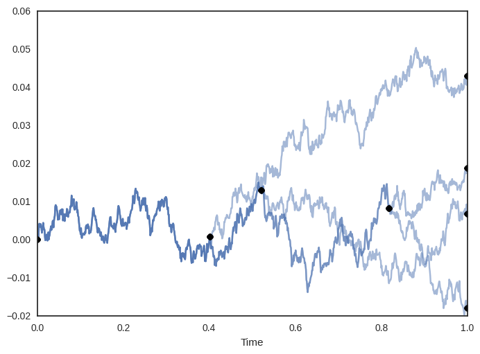
The Dirichlet diffusion tree (DDT) is a generative model for -dimensional vectors . Data are generated sequentially via a continuous-time process, lasting from time to , whereupon they reach their final value.
The first point, , is generated via a Brownian motion, beginning at the origin, i.e. where represents the value of at time . The next point, , follows the path created by until it eventually diverges at a random time, according to a specified acquisition function . When diverges, it creates an internal node in the tree structure which contains both the time and value of when it diverged. After divergence, it continues until with an independent Brownian motion. In general, the -th point follows the path created by the previous points. When it reaches a node, it will first sample one of two branches to enter, then either 1) diverge on the branch, whereupon a divergence time is sampled according to the acquisition function , or 2) recursively continue to the next node. Each of these choices has a probability associated with it, according to various properties of the tree structure and choice of acquisition function (details can be found in Neal (2003)). Eventually, all points will diverge and continue independently, creating an internal node storing the time and intermediate value for each point at divergence. The DDT thus defines a binary tree over the data (see Figure 1 for an example). Furthermore, given a DDT with points, it is possible to sample the possible divergence locations of a -th point, using the generative process.
Sampling the posterior DDT given data can be done with the Metropolis-Hastings (MH) algorithm, an MCMC method. The MH algorithm obtains samples from target distribution indirectly by instead sampling from a conditional “proposal” distribution , creating a Markov chain whose stationary distribution is , assuming satisfies some conditions. Our choice of proposal distribution modifies the DDT’s tree structure via a subtree-prune and regraft (SPR) move, which has the added benefit of extending to other distributions over hierarchies.
The Subtree-Prune and Regraft Move
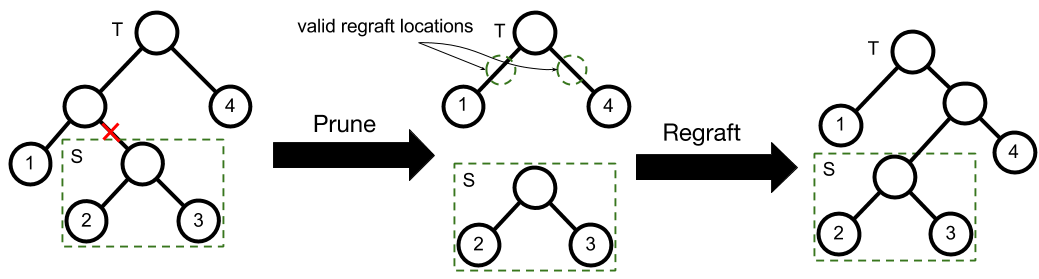
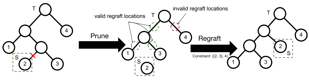
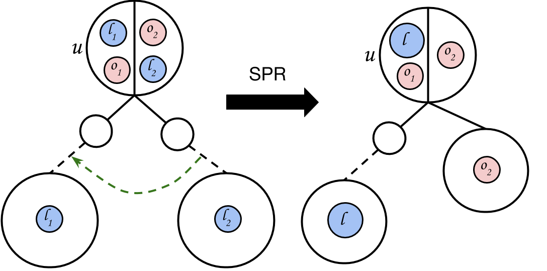
An SPR move consists of first a prune then a regraft. Suppose is a binary tree with leaves. Let be a non-root node in selected uniformly at random and be its corresponding subtree. To prune from , we remove ’s parent from , and replace with ’s sibling.
Regrafting selects a branch at random and attaches to it as follows. Let be the chosen branch ( is the parent of ). is attached to the branch by creating a node with children and and parent (see Figure 2 for an example).
The MH proposal distribution for the DDT is an augmented SPR move, where the time and intermediate value at each node are sampled in addition to tree structure. The exchangeability of the DDT enables efficient sampling of regraft branches by simulating the generation process for a new point and returning the branch and time where it diverges. The intermediate values for the entire tree are sampled via an interleaved Gibbs sampling move, as all conditional distributions are Gaussian.
3 Adding interaction
Impressive as the Dirichlet diffusion tree is, there is no reason to suppose that it will magically find a tree that suits the user’s needs. But a little interaction can be helpful in improving the outcome.
Let denote the target hierarchical clustering. It is not necessarily the case that the user would be able to write this down explicitly, but this is the tree that captures the distinctions he/she is able to make, or wants to make. Figure 3 (left) shows an example, for a small data set of 5 points. In this case, the user does not wish to distinguish between points , but does wish to place them in a cluster that excludes point .
We could posit our goal as exactly recovering . But in many cases, it is good enough to find a tree that captures all the distinctions within but also possibly has some extraneous distinctions, as in the right-hand side of Figure 3.
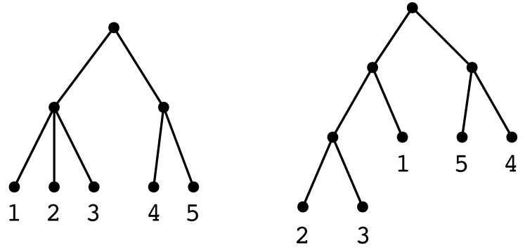
Formally, given data set , we say is a cluster of tree if there is some node of whose descendant leaves are exactly . We say is a refinement of if they have the same set of leaves, and moreover every cluster of is also a cluster of . This, then, is our goal: to find a refinement of the target clustering .
3.1 Triplets
The user provides feedback in the form of triplets. The constraint means that the tree should have a cluster containing and but not . Put differently, the lowest common ancestor of should be a strict descendant of the lowest common ancestor of .
Let denote the set of all proper triplet constraints embodied in tree . If has nodes, then . For non-binary trees, it will be smaller than this number. Figure 3 (left), for instance, has no triplet involving .
Refinement can be characterized in terms of triplets.
Lemma 3.1.
Tree is a refinement of tree if and only if .
Proof.
See supplement. ∎
In particular, any triplet-querying scheme that converges to the full set of triplets of the target tree is also guaranteed to produce trees that converge to a refinement of .
With this lemma in mind, it is natural to measure how close a tree is to the target with the following (asymmetric) distance function, which we call triplet distance (TD):
| (1) |
where is the indicator function. This distance is zero exactly when is a refinement of , in which case we have reached our goal.
A simple strategy for obtaining triplets would be to present the user with three randomly chosen data points and have the user pick the odd one out. This strategy has several drawbacks. First, some sets of three points have no triplet constraint (for instance, points in Figure 3). Second, the chosen set of points might correspond to a triplet that has already been specified, or is implied by specified triplets. For example, knowledge of and implies . Enumerating the set of implied triplets is non-trivial for triplets (Bryant & Steel, 1995), making it difficult to avoid these implied triplets in the first place.
We thus consider another strategy—rather than the user arranging three data points into a triplet, the user observes the hierarchy induced over some -sized subset of the data and corrects an error in the tree by supplying a triplet. We call this is a subtree query. Finally, we note that in this work we only consider the realizable case where the triplets obtained from a user do not contain contradictory information and that there is a tree that satisfies all of them.
3.2 Finding a tree consistent with constraints
We start with a randomly initialized hierarchy over our data and show an induced subtree to the user, obtaining the first triplet. The next step is constructing a new tree that satisfies the triplet. This begins the feedback cycle; a user provides a triplet given a subtree and the triplet is incorporated into a clustering algorithm, producing a new candidate tree. A starting point is an algorithm that returns a tree consistent with a set of triplets.
The simplest algorithm to solve this problem is the BUILD algorithm, introduced in Aho et al. (1981). Given a set of triplets , BUILD will either return a tree that satisfies , or error if no such tree exists. In BUILD, we first construct the Aho graph , which has a vertex for each data point and an undirected edge for each triplet constraint . If is connected, there is no tree that satisfies all triplets. Otherwise, the top split of the tree is a partition of the connected components of : any split is fine as long as points in the same component stay together. Satisfied triplets are discarded, and BUILD then continues recursively on the left and right subtrees.
BUILD satisfies triplet constraints but ignores the geometry of the data, whereas we wish to take both into account. By incorporating triplets into the posterior DDT sampler, we obtain high likelihood trees that still satisfy .
3.3 Incorporating triplets into the sampler
In this section, we present an algorithm to sample candidate trees from the posterior DDT, constrained by a triplet set . It is based on the subtree prune and regraft move.
The SPR move is of particular interest because we can efficiently enforce triplets to form a constrained-SPR move, resulting in a sampler that only produces trees that satisfy a set of triplets. A constrained-SPR move is defined as an SPR move that assigns zero probability to any resulting trees that would violate a set of triplets. Restricting the neighborhood of an SPR move runs the risk of partitioning the state space, losing the convergence guarantees of the Metropolis-Hastings algorithm. Fortunately, a constrained-SPR move does not compromise strong connectivity. For any realizable triplet set , we prove the constrained-SPR move Markov chain’s aperiodicity and irreducibility.
Consider the Markov chain on the state space of rooted binary trees that is induced by the constrained sampler.
Lemma 3.2.
The constrained-SPR Markov chain is aperiodic.
Proof.
A sufficient condition for aperiodicity is the existent of a “self-loop” in the transition matrix: a non-zero probability of a state transitioning to itself. Supposed we have pruned a subtree already. When regrafting, the ordinary SPR move has a non-zero probability of choosing any branch, and a constrained-SPR move cannot regraft to branches that would violate triplets. Since the current tree in the Markov chain satisfies triplet set , there is a non-zero probability of regrafting to the same location. We thus have an aperiodic Markov chain. ∎
Lemma 3.3.
A constrained-SPR Markov chain is irreducible.
Proof.
(sketch) To show irreducibility, we show that a tree has an non-zero probability of reaching an arbitrary tree via constrained-SPR moves where both and satisfy a set of triplets . Our proof strategy is to construct a canonical tree , and show that there exists a non-zero probability path from to , and therefore from to . We then show that for a given constrained-SPR move, the reverse move has a non-zero probability. Thus, there exists a path from to to , satisfying irreducibility.
Recall that the split at a node in a binary tree that satisfies triplet set corresponds to a binary partition of the Aho graph at the node (see Section 3.2). is a tree such that every node in is in canonical form. A node is in canonical form if it is a leaf node, or, the partition of the Aho graph at that node can be written as . is the single connected component containing the point with the minimum data index, and is the rest of the components.
To convert a particular node into canonical form, we first perform “grouping”, which puts into a single descendant of via constrained-SPR moves. We then make two constrained-SPR moves to convert the partition at into the form (see Figure 5). We convert all nodes into canonical form recursively, turning an arbitrary tree into .
Finally, the reverse constrained-SPR move has a non-zero probability. Suppose we perform a constrained-SPR move on tree , converting it into by detaching subtree and attaching it to branch . A constrained-SPR move on can select for pruning and can regraft it to form with a non-zero probability since satisfies the same constraint set as . For a full proof, please refer to the supplement. ∎
The simplest possible scheme for a constrained-SPR move would be rejection sampling. The Metropolis-Hastings algorithm for the DDT would be the same as in the unconstrained case, but any trees violating would have accept probability . Although this procedure is correct, it is impractical. As the number of triplets grows larger, more trees will be rejected and the sampler will slow down over time.
To efficiently sample a tree that satisfies a set of triplets , we modify the regraft in the ordinary SPR move. The constrained-SPR move must assign zero probability to any regraft branches that would result in a tree that violates . This is accomplished by generating the path from the root in the same manner as sampling a branch, but avoiding paths that would resulted in violated triplets.
Description of constrained-SPR sampler
Recall that in the DDT’s sampling procedure for regraft branches, a particle at a node picks a branch, and either diverges from that branch or recursively samples the node’s child. Let be the root of the subtree we are currently grafting back onto tree , let be the triplet set, and let denote the descendant-leaves of node . Suppose we are are currently at node , deciding whether to diverge at the branch or to recursively sample . Consider any triplet . If all—or none—of are in , then the triplet is unaffected by the graft, and can be ignored. Otherwise, some checks are needed:
-
1.
Then we know . If and are split across ’s children, we are banned from sampling .
-
2.
but
If both and are in , we are required to sample . If just is in , we are banned from both diverging at and sampling . Otherwise we can either diverge at or sample .
(The case where is symmetric to case 2.) If we choose to sample , we remove constraints from our current set that are now satisfied, and continue recursively. This defines a procedure by which we can sample a divergence branch that does not violate constraints.
While the constrained-SPR sampler can produce a set of trees given a set of static constraints, the BUILD algorithm is useful in adding new triplets into the sampler. Suppose we have been sampling trees with constrained-SPR moves with satisfying triplet set and we obtain a new triplet from a user query. We take the current tree and find the least common ancestor (call it ) of and . We then call BUILD on just the nodes in , and we substitute the resulting subtree at position in tree .
3.4 Intelligent subset queries
We now have a method to sample a constrained distribution over candidate trees. Given a particular candidate tree , our first strategy for subtree querying is to pick a random subset of the leaves of constant size, and show the user the induced subtree over the subset, . We call this random subtree querying. But can we use a set of trees produced by the sampler to make better subtree queries? If tree structure is ambiguous in a particular region of data, i.e. there are several hierarchies that could explain a particular configuration of data, the MH algorithm will sample over these different configurations. A query over points in these ambiguous regions may help our algorithm converge to a better tree faster. By looking for these regions in our samples, we can choose query subsets for which the tree structure is highly variable, and hopefully the resulting triplet from the user will reduce the ambiguity.
More precisely, we desire a notion of tree variance. Given a set of trees , what is the variance over a given subset of the data ? We propose using the notion of tree distance as a starting point. For a given tree , the tree distance between two nodes and , denoted , is the number of edges of needed to get from to . Consider two leaves and . If the tree structure around them is static, we expect the tree distance between and to change very little, as the surrounding tree will not change. However, if there is ambiguity in the surrounding structure, the tree distance will be more variable. Given a subset of data and a set of trees , the tree distance variance (TDV) of the trees over the subset is defined as:
| (2) |
This measure of variance is the max of the variance of tree distance between any two points in the subset. Computing this requires time, and since since is constant, it is not prohibitively expensive.
Given a set of trees from the sampler , we now select a high-variance subtree by instantiating random subsets of constant size, and picking . We call this active subtree querying. Although using tree variance will help reconcile ambiguity in the tree structure, if a set of samples from a tree all violate the same triplet, it is unlikely that active querying will recover that triplet. Thus, interleaving random querying and active querying will hopefully help the algorithm converge quickly, while avoiding local optima.
4 Experiments
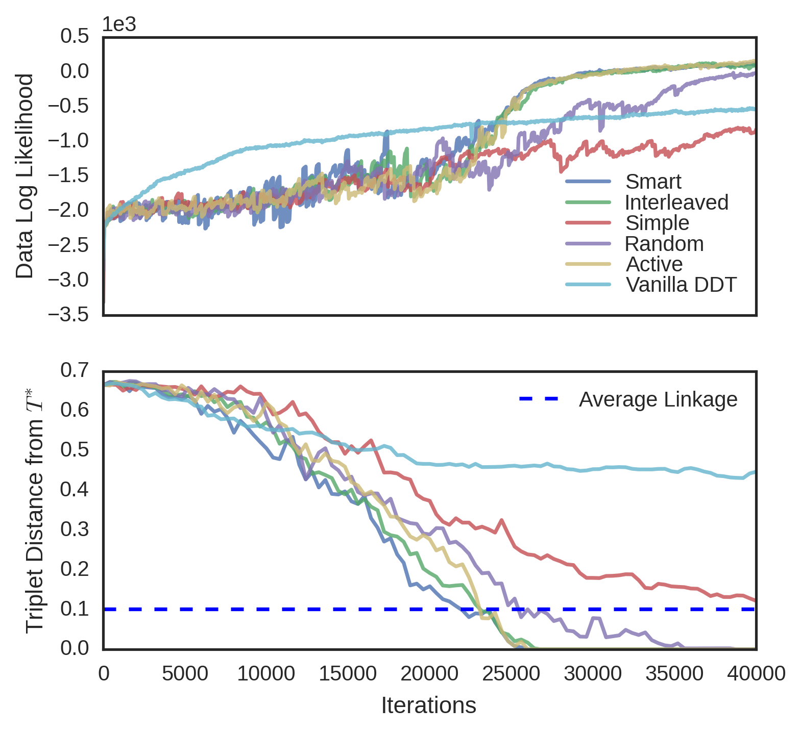
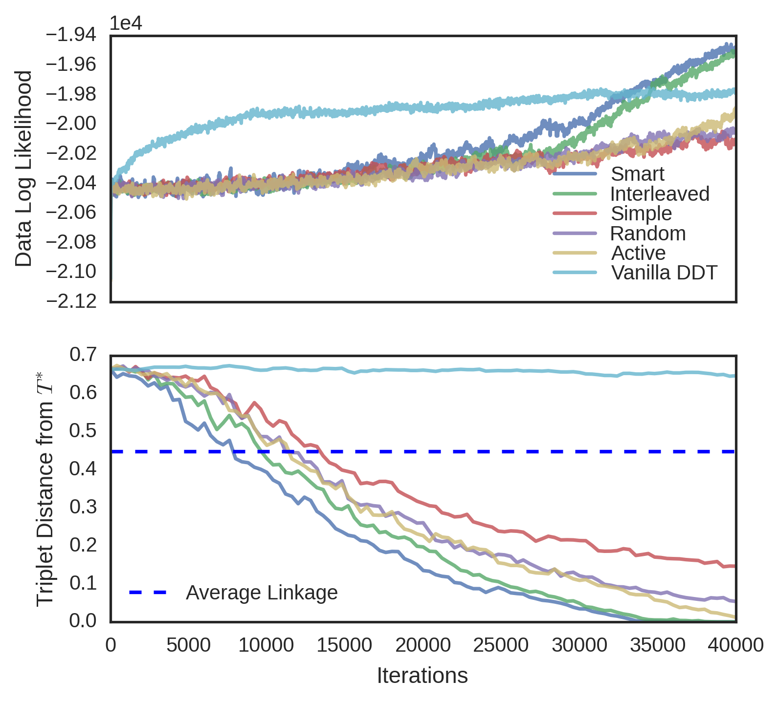
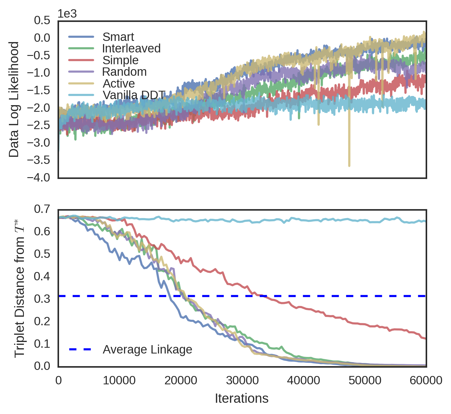
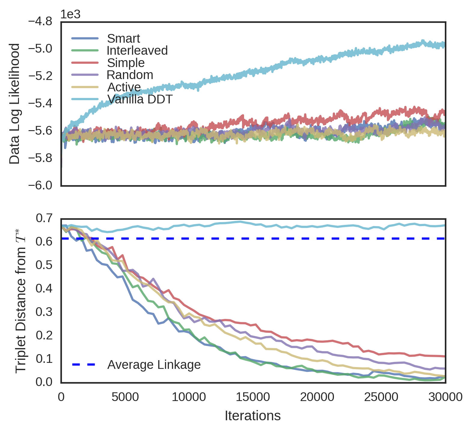
We evaluated the convergence properties of five different querying schemes. In a “simple query”, a user is presented with three random data and picks an odd one out. In a “smart query”, a user is unrealistically shown the entire candidate tree and reports a violated triplet. In a “random query”, the user is shown the induced candidate tree over a random subset of the data. In an “active query”, the user is shown a high variance subtree using tree-distance variance. Finally, in an “interleaved query”, the user is alternatively shown a random subtree and a high variance subtree. In each experiment, was known, so user queries were simulated by picking a triplet violated by the root split of the queried tree, and if no such triplet existed, recursing on a child. Each scheme was evaluated on four different datasets. The first dataset, MNIST (Lecun et al., 1998), is an 10-way image classification dataset where the data are 28 x 28 images of digits. The target tree is simply the -way classification tree over the data. The second dataset is Fisher Iris, a 3-way flower classification problem, where each of 150 flowers has five features. The third dataset, Zoo (Lichman, 2013), is a set of 93 animals and 15 binary morphological features for each of animals, the target tree being the induced binary tree from the Open Tree of Life (Hinchliff et al., 2015). The fourth dataset is 20 Newsgroups (Joachims, 1997), a corpus of text articles on 20 different subjects. We use the first 10 principal components as features in this classification problem. All datasets were modeled with DDT’s with acquisition function and Brownian motion parameter estimated from data. To better visualize the different convergence rates of the querying schemes, MNIST and 20 Newsgroups were subsampled to 150 random points.
For each dataset and querying scheme, we instantiated a SPR sampler with no constraints. Every one hundred iterations of the sampler, we performed a query. In subtree queries, we used subsets of size and in active querying, the highest-variance subset was chosen from different random subsets. As baselines, we measured the triplet distance of the vanilla DDT and the average linkage tree. Finally, results were averaged over four runs of each sampler. The triplet distances for Fisher Iris and MNIST can be seen in Figure 6. Results for the other datasets can be found in the supplement. Although unrealistic due to the size of the tree shown to the user, the smart query performed the best, achieving minimum error with the least amount of queries. Interleaved followed next, followed by active, random, and simple. In general, the vanilla DDT performed the worst, and the average linkage score varied on each dataset, but in all cases, the subtree querying schemes performed better than both the vanilla DDT and average linkage.
In three datasets (MNIST, Fisher Iris and Zoo), interactive methods achieve higher data likelihood than the vanilla DDT. Initially, the sampler is often restructuring the tree with new triplets and data likelihood is unlikely to rise. However, over time as less triplets are reported, the data likelihood increases rapidly. We thus conjecture that triplet constraints may help the MH algorithm find better optima.
5 Future Work
We are interested in studying the non-realizable case, i.e. when there does not exist a tree that satisfies triplet set . We would also like to better understand the effect of constraints on searching for optima using MCMC methods.
References
- Adams et al. (2008) Adams, R.P., Ghahramani, Z., and Jordan, M.I. Tree-structured stick breaking for hierarchical data. In Advances in Neural Information Processing Systems, 2008.
- Aho et al. (1981) Aho, A.V., Sagiv, Y., Szymanski, T.G., and Ullman, J.D. Inferring a tree from lowest common ancestors with an application to the optimization of relational expressions. SIAM Journal on Computing, 10:405–421, 1981.
- Aldous (1995) Aldous, D. Probability distributions on cladograms. In Aldous, D. and Pemantle, R. (eds.), Random Discrete Structures (IMA Volumes in Mathematics and its Applications 76), pp. 1–18, 1995.
- Awasthi & Zadeh (2010) Awasthi, P. and Zadeh, R.B. Supervised clustering. In Advances in Neural Information Processing Systems, 2010.
- Awasthi et al. (2014) Awasthi, P., Balcan, M.-F., and Voevodski, K. Local algorithms for interactive clustering. In Proceedings of the 31st International Conference on Machine Learning, 2014.
- Balcan & Blum (2008) Balcan, M.-F. and Blum, A. Clustering with interactive feedback. In Algorithmic Learning Theory (volume 5254 of the series Lecture Notes in Computer Science), pp. 316–328, 2008.
- Bansal et al. (2004) Bansal, N., Blum, A., and Chawla, S. Correlation clustering. Machine Learning, 56(1–3):89–113, 2004.
- Basu et al. (2004) Basu, S., Banerjee, A., and Mooney, R. Active semi-supervision for pairwise constrained clustering. In SIAM International Conference on Data Mining, 2004.
- Biswas & Jacobs (2014) Biswas, A. and Jacobs, D. Active image clustering with pairwise constraints from humans. International Journal of Computer Vision, 108(1):133–147, 2014.
- Borg & Groenen (2005) Borg, I. and Groenen, P.J.F. Modern Multidimensional Scaling: Theory and Applications. Springer Verlag, 2005.
- Boyles & Welling (2012) Boyles, L. and Welling, M. The time-marginalized coalescent prior for hierarchical clustering. In Advances in Neural Information Processing Systems, 2012.
- Bryant & Steel (1995) Bryant, D and Steel, M. Extension operations on sets of leaf-labeled trees. Advances in Applied Mathematics, 16(4):425–453, 1995.
- Eriksson et al. (2011) Eriksson, B., Dasarathy, G., Singh, A., and Nowak, R. Active clustering: robust and efficient hierarchical clustering using adaptively selected similarities. In Proceedings of the 14th International Conference on Artificial Intelligence and Statistics, 2011.
- Felsenstein (2004) Felsenstein, J. Inferring Phylogenies. Sinauer, 2004.
- Hastie et al. (2009) Hastie, T., Tibshirani, R., and Friedman, J. The Elements of Statistical Learning. Springer, 2nd edition, 2009.
- Heller & Ghahramani (2005) Heller, K. and Ghahramani, Z. Bayesian hierarchical clustering. In Proceedings of the 22nd International Conference on Machine Learning, 2005.
- Hinchliff et al. (2015) Hinchliff, Cody E., Smith, Stephen A., Allman, James F., Burleigh, J. Gordon, Chaudhary, Ruchi, Coghill, Lyndon M., Crandall, Keith A., Deng, Jiabin, Drew, Bryan T., Gazis, Romina, Gude, Karl, Hibbett, David S., Katz, Laura A., Laughinghouse, H. Dail, McTavish, Emily Jane, Midford, Peter E., Owen, Christopher L., Ree, Richard H., Rees, Jonathan A., Soltis, Douglas E., Williams, Tiffani, and Cranston, Karen A. Synthesis of phylogeny and taxonomy into a comprehensive tree of life. In Proceedings of the National Academy of Sciences, 2015.
- Joachims (1997) Joachims, Thorsten. A probabilistic analysis of the rocchio algorithm with tfidf for text categorization. In Proceedings of the Fourteenth International Conference on Machine Learning, ICML ’97, pp. 143–151, 1997. ISBN 1-55860-486-3.
- Knowles & Ghahramani (2015) Knowles, D.A. and Ghahramani, Z. Pitman-Yor diffusion trees for Bayesian hierarchical clustering. IEEE Transactions on Pattern Analysis and Machine Intelligence, 37(2):271–289, 2015.
- Krishnamurthy et al. (2012) Krishnamurthy, A., Balakrishnan, S., Xu, M., and Singh, A. Efficient active algorithms for hierarchical clustering. In Proceedings of the 29th International Conference on Machine Learning, 2012.
- Kulis et al. (2005) Kulis, B., Basu, S., Dhillon, I., and Mooney, R. Semi-supervised graph clustering: a kernel approach. In Proceedings of the 22nd International Conference on Machine Learning, 2005.
- Lecun et al. (1998) Lecun, Yann, Bottou, Léon, Bengio, Yoshua, and Haffner, Patrick. Gradient-based learning applied to document recognition. In Proceedings of the IEEE, pp. 2278–2324, 1998.
- Lichman (2013) Lichman, M. UCI machine learning repository, 2013. URL http://archive.ics.uci.edu/ml.
- McCullagh et al. (2008) McCullagh, P., Pitman, J., and Winkel, M. Gibbs fragmentation trees. Bernoulli, 14(4):988–1002, 2008.
- Neal (2003) Neal, R.M. Density modeling and clustering using Dirichlet diffusion trees. In Bernardo, J.M. et al. (eds.), Bayesian Statistics 7, pp. 619–629. Oxford University Press, 2003.
- Tamuz et al. (2011) Tamuz, O., Liu, C., Belongie, S., Shamir, O., and Kalai, A.T. Adaptively learning the crowd kernel. In Proceedings of the 28th International Conference on Machine Learning, 2011.
- Teh et al. (2008) Teh, Y.W., III, H. Daume, and Roy, D.M. Bayesian agglomerative clustering with coalescents. In Advances in Neural Information Processing Systems, 2008.
- Wagstaff & Cardie (2000) Wagstaff, K. and Cardie, C. Clustering with instance-level constraints. In Proceedings of the 17th International Conference on Machine Learning, 2000.
- Wagstaff et al. (2001) Wagstaff, K., Cardie, C., Rogers, S., and Schroedl, S. Constrained k-means clustering with background knowledge. In Proceedings of the 18th International Conference on Machine Learning, 2001.
- Williams (2000) Williams, C.K.I. A MCMC approach to hierarchical mixture modeling. In Advances in Neural Information Processing Systems, 2000.
- Zoller & Buhmann (2000) Zoller, T. and Buhmann, J.M. Active learning for hierarchical pairwise data clustering. In Proceedings of the 15th International Conference on Pattern Recognition, 2000.
Appendix A Proof Details
See 3.1
Proof.
Suppose, first, that is a refinement of . Pick any triplet . Then there is a node in whose descendants include but not . By the definition of refinement, contains a node with the same descendants. Hence the constraint holds for as well.
Conversely, say . Pick any cluster of ; it consists of the descendants of some node in . Consider the set of all triplet constraints consisting of two nodes of and one node outside . Since these constraints also hold for , it follows that the lowest common ancestor of in must have exactly as its set of descendants. Thus is also a cluster of . ∎
See 3.3
Proof.
To prove irreducibility, we show that there is a non-zero probability of moving from state to , both of which satisfy . We accomplish this by first defining a canonical tree given a triplet set and showing that we can reach from using constrained-SPR moves. We then show that for every constrained-SPR move, there exists an equivalent reverse move that undoes it with non-zero probability. This proves that that from we can reach , creating a path from to to .
A binary tree can be entirely defined by the bipartitions made over the data at each node. Let be the Aho graph for node . For a binary tree that satisfies a set of triplets, the split over the data at each node must be a bipartition of the connected components of . We define a particular node to be in canonical form if either a) it is a leaf, or b) the bipartition over at that node can be written as , where exactly matches a single, particular connected component of , and is the rest of the connected components. The particular component is the connected component in with the minimum data index inside it. Note that we treat the children of nodes as unordered. A canonical tree is one such that every node in the tree is in canonical form. To convert an arbitrary tree that satisfies into , we first convert the root node of into canonical form using constrained-SPR moves.
Let be the root of and let be the set of points that ought to be in their own partition according to . In order for not to be in canonical form, must be in a partition with data from other connected components in , which we will call . The bipartition if were in canonical form would be and the current non-canonical bipartition can thus be written as .
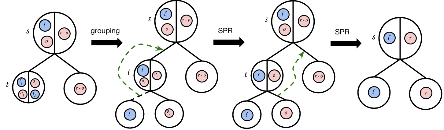
We first examine , the child of the root that contains . In general, the data from and the data from could be split over the children of , so the partition at can be written as where and . This is visualized in the first tree of Figure 5. We first group the data from into their own “pure” subtree of as follows. Let be the root of the lowest non-pure subtree of that has data from in both of its children. There exist two subtrees that are descendants of that contain data from (one on the left and one on the right). Those two subtrees must be pure, and furthermore, they are both free to move within via constrained-SPR moves because they are in different connected components in . Thus, we can perform a constrained-SPR move to merge these two pure subtrees together into a larger pure subtree. We can repeat this process for until all nodes from are in their own pure subtree of . The partition of can thus be written as , since the pure subtree may be several levels down from . This grouping process is visualized in Figure S1 and the results can be seen in the second tree in Figure 5.
We now perform a constrained-SPR move to detach the pure subtree of and regraft it to the edge between and . This is a permissible move since is its own connected component in . We now have the third tree in Figure S2. We now perform a final constrained-SPR move, moving the subtree of to the opposite side of , creating the proper canonical partition of . To entirely convert into , we need to recurse and convert every node in into canonical form.
Every constrained-SPR move has an associated reverse constrained-SPR move that performs the opposite transition. The reverse constrained-SPR move selects the same subtree as the forward one and prunes it, and just regrafts the subtree to its original location before the forward move. We know that this regraft has non-zero probability because the original tree did not violate constraints. Thus, since any arbitrary can be converted into and since each move has a non-zero probability reverse move, can be converted into an arbitrary tree and we have a non-zero probability path to convert into .
∎
Appendix B Additional Results