Interference Cancelation in Coherent CDMA Systems Using Parallel Iterative Algorithms
Abstract
Least mean square-partial parallel interference cancelation (LMS-PPIC) is a partial interference cancelation using adaptive multistage structure in which the normalized least mean square (NLMS) adaptive algorithm is engaged to obtain the cancelation weights. The performance of the NLMS algorithm is mostly dependent to its step-size. A fixed and non-optimized step-size causes the propagation of error from one stage to the next one. When all user channels are balanced, the unit magnitude is the principal property of the cancelation weight elements. Based on this fact and using a set of NLMS algorithms with different step-sizes, the parallel LMS-PPIC (PLMS-PPIC) method is proposed. In each iteration of the algorithm, the parameter estimate of the NLMS algorithm is chosen to match the elements’ magnitudes of the cancelation weight estimate with unity. Simulation results are given to compare the performance of our method with the LMS-PPIC algorithm in three cases: balanced channel, unbalanced channel and time varying channel.
I Introduction
Multiuser detectors for code division multiple access (CDMA) receivers are effective techniques to eliminate the multiple access interference (MAI). In CDMA systems, all users receive the whole transmitted signals concurrently that are recognized by their specific pseudo noise (PN) sequences. In such a system, there exists a limit for the number of users that are able to simultaneously communicate. This limitation is because of the MAI generated by other users (see e.g. [1, 2]). High quality detectors improve the capacity of these systems [1, 6]. However their computational complexities grow exponentially with increasing the number of users and the length of the transmitted sequence [7].
Multiple stage subtractive interference cancelation is a suboptimal solution with reduced computational complexity. In this method and before making data decisions, the estimated interference from other users are removed from the specific user’s received signal. The cancelation can be carried out either in a serial way (successively) (see e.g. [8, 9]) or in a parallel manner (see e.g. [3, 2, 10]). The parallel interference cancelation (PIC) is a low computational complex method that causes less decision delay compared to the successive detection and is much simpler in implementation.
Usually at the first stage of interference cancelation in a multiple stage system, the interfering data for each user which is made by other users is unknown. PIC is implemented to estimate this data stage by stage. In fact when MAI is estimated for each user, the bit decision at the stage of cancelation are used for bit detection at the stage. Apparently, the more accurate the estimates are, the better performance of the detector is. However, in the conventional multistage PIC [3], a wrong decision in one stage can increase the interference. Based on minimizing the mean square error between the received signal and its estimate from the previous stage, G. Xue et al. proposed the least mean square-partial parallel interference cancelation (LMS-PPIC) method [10, 11]. In LMS-PPIC, a weighted value of MAI of other users is subtracted before making the decision of a specific user. The least mean square (LMS) optimization and the normalized least mean square (NLMS) algorithm [13] shape the structure of the LMS-PPIC method of the weight estimation of each cancelation stage. However, the performance of the NLMS algorithm is mostly dependent on its step-size. Although a large step-size results in a faster convergence rate, but it causes a large maladjustment. On the other hand, with a very small step-size, the algorithm almost keeps its initial values and can not estimate the true cancelation weights. In the LMS-PPIC method, both of these cases cause propagation of error from one stage to another. In LMS-PPIC, the element of the weight vector in each stage is the true transmitted binary value of the user divided by its hard estimate value from the previous stage. Hence the magnitude of all weight elements in all stages are equal to unity. This is a valuable information that can be used to improve the performance of the LMS-PPIC method. In this paper, we propose parallel LMS-PPIC (PLMS-PPIC) method by using a set of NLMS algorithms with different step-sizes. The step-size of each algorithm is chosen from a sharp range [14] that guarantees stable operation. While in this paper we assume coherent transmission, the non-coherent scenario is investigated in [5].
The rest of this paper is organized as follows: In section II, the LMS-PPIC [10] is reviewed. The LMS-PPIC algorithm is an important example of multistage parallel interference cancelation methods. In section III, the PLMS-PPIC method is explained. In section IV some simulation examples are given to compare the results of PLMS-PPIC with those of LMS-PPIC. Finally, the paper is concluded in section V.
II Multistage Parallel Interference Cancelation: LMS-PPIC Method
We assume users synchronously send their symbols via a base-band CDMA transmission system where . The user has its own code of length , where , for all . It means that for each symbol bits are transmitted by each user and the processing gain is equal to . At the receiver we assume that perfect power control scheme is applied. Without loss of generality, we also assume that the power gains of all channels are equal to unity and users’ channels do not change during each symbol transmission (it can change from one symbol transmission to the next one) and the channel phase of user is known for all (see [5] for non-coherent transmission). We define
| (1) |
According to the above assumptions, the received signal is
| (2) |
where is additive white Gaussian noise with zero mean and variance . In order to make a new variable set for the current stage , multistage parallel interference cancelation method uses (the bit estimate outputs of the previous stage ) to estimate the related MAI of each user, to subtract it from the received signal and to make a new decision on each user variable individually. The output of the last stage is considered as the final estimate of the transmitted bits. In the following we explain the structure of the LMS-PIC method. Assume is a given estimate of from stage . Let us define
| (3) |
| (4) |
Define
| (5a) | |||||
| (5b) | |||||
where stands for transposition. From equations (4), (5a) and (5b), we have
| (6) |
Given the observations , an adaptive algorithm can be used to compute
| (7) |
which is an estimate of after iterations. Then , the estimate of at stage , is given by
| (8) |
where stands for complex conjugation and
| (9) |
The inputs of the first stage (needed for computing ) is given by the conventional bit detection
| (10) |
Given the available information and using equation (6), there are a variety of choices for parameter estimation. In LMS-PPIC, the NLMS algorithm is used to compute . Table I shows the full structure of the LMS-PPIC method.
To improve the performance of the LMS-PPIC method, in the next section we propose a modified version of it. In our method a set of individual NLMS algorithms with different step-sizes are used.
III Multistage Parallel Interference Cancelation: PLMS-PPIC Method
The NLMS (with fixed step-size) converges only in the mean sense. In the literature, guarantees the mean convergence of the NLMS algorithm [13, 15]. Based on Cramér-Rao bound, a sharper range was given in [14] as follows
| (11) |
where is the length of the parameter under estimate. Here is the number of users or equivalently the system load. As equation (11) shows, the range of the step-size is a decreasing function of the system load. It means that as the number of users increases, the step-size must be decreased and vice versa. In the proposed PLMS-PPIC method, has a critical role.
From (3), we have
| (12) |
which is equivalent to
| (13) |
To improve the performance of the NLMS algorithm, at time iteration , we can determine the step size from , in such a way that is minimized, i.e.
| (14) |
where , the element of , is given by (see Table I)
| (15) |
The complexity to determine from (14) is high, especially for large values of . Instead we propose the following method.
We divide into subintervals and consider individual step-sizes , where , and . In each stage, individual NLMS algorithms are executed ( is the step-size of the algorithm). In stage and at iteration , if , the parameter estimate of the algorithm minimized our criteria, i.e.
| (16) |
where and , then it is considered as the parameter estimate at time iteration , i.e. and all other algorithms replace their weight estimates by . Table II shows the details of the PLMS-PPIC method. As Table II shows, in stage and at time iteration where is computed, the PLMS-PPIC method computes from equation (8). This is similar to the LMS-PPIC method. Here the PLMS-PPIC and the LMS-PPIC methods are compared with each other.
-
•
Computing , times more than LMS-PPIC, and computing in each iteration of each stage of PLMS-PPIC, is the difference between it and the LMS-PPIC method.
-
•
Because the step-sizes of all individual NLMS algorithms of the proposed method are given from a stable operation range, all of them converge fast or slowly. Hence the PLMS-PPIC is a stable method.
-
•
As we expected and our simulations show, choosing the step-size as a decreasing function of system loads (based on relation (11)) improves the performance of both NLMS algorithm in LMS-PPIC and parallel NLMS algorithms in PLMS-PPIC methods in such a way that there is no need for the third stage, i.e. both the LMS-PPIC and PLMS-PPIC methods get the optimum weights in the second stage. However only when the channel is time varying, the third stage is needed, e.g. 3.
-
•
Increasing the number of parallel NLMS algorithms in PLMS-PPIC method increases the complexity, while it improves the performance as well.
-
•
As our simulations show, the LMS-PPIC method is more sensitive to the Channel loss, near-far problem or unbalanced channel gain compared to the PLMS-PPIC.
In the following section, some examples are given to illustrate the effectiveness of our proposed methods.
IV Simulations
In this section we have considered some simulation examples. Examples 1-3 compare the conventional, the LMS-PPIC and the PLMS-PPIC methods in three cases: balanced channels, unbalanced channels and time varying channels. Example 1 is given to compare LMS-PPIC and PLMS-PPIC in the case of balanced channels.
Example 1
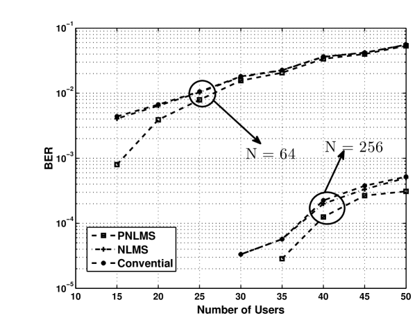
Balanced channels: Consider the system model (4) in which users, each having their own codes of length , send their own bits synchronously to the receiver and through their channels. The signal to noise ratio (SNR) is dB. In this example we assume that there is no power-unbalanced or channel loss. The step-size of the NLMS algorithm in LMS-PPIC method is and the set of step-sizes of the parallel NLMS algorithms in PLMS-PPIC method is , i.e. . Figure 1 shows the average bit error rate (BER) over all users versus , using two stages when and . As it is shown, while there is no remarkable performance difference between all three methods for , the PLMS-PPIC outperforms the conventional and the LMS-PPIC methods for . Simulations also show that there is no remarkable difference between results in two stage and three stage scenarios.
Although LMS-PPIC and PLMS-PPIC are structured based on the assumption of no near-far problem, these methods (especially the second one) have remarkable performance in the cases of unbalanced and/or time varying channels. These facts are shown in the two upcoming examples.
Example 2
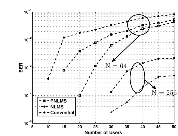
Unbalanced channels: Consider example 1 with power unbalance and/or channel loss in transmission system, i.e. the true model at stage is
| (17) |
where for all . Both the LMS-PPIC and the PLMS-PPIC methods assume the model (4), and their estimations are based on observations , instead of , where the channel gain matrix is . In this case we repeat example 1. We randomly get each element of from . Results are given in Figure 2. As it is shown, in all cases the PLMS-PPIC method outperforms both the conventional and the LMS-PPIC methods.
Example 3
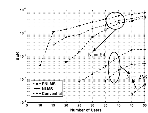
Time varying channels: Consider example 1 with time varying Rayleigh fading channels. In this case we assume the maximum Doppler shift of HZ, the three-tap frequency-selective channel with delay vector of sec and gain vector of dB. Results are given in Figure 3. As it is seen while the PLMS-PPIC outperforms the conventional and the LMS-PPIC methods when the number of users is less than , all three methods have the same performance when the number of users is greater than .
V Conclusion
In this paper, parallel interference cancelation using adaptive multistage structure and employing a set of NLMS algorithms with different step-sizes is proposed. According to the proposed method, in each iteration the parameter estimate is chosen in a way that its corresponding algorithm has the best compatibility with the true parameter. Because the step-sizes of all algorithms are chosen from a stable range, the total system is therefore stable. Simulation results show that the new method has a remarkable performance for different scenarios including Rayleigh fading channels even if the channel is unbalanced.
References
- [1] S. Verdú, Multiuser Detection, Cambridge University Press, 1998.
- [2] D. Divsalar, M. K. Simon and D. Raphaeli, “Improved parallel inteference cancellation for CDMA,” IEEE Trans. Commun., vol. COM-46, no. 2, pp. 258-268, Feb. 1998.
- [3] M. K. Varanasi and B. Aazhang, “Multistage detection in asynchronous code division multiple-access communication,”IEEE trans. Commun., vol. COM-38, no 4, pp.509-519, April 1990.
- [4] S. Verdú, “Minimum probability of error for asynchronous Gaussian multiple-access channels,” IEEE Trans. Inform. Theory, vol. IT-32, pp. 85-96, Jan. 1986.
- [5] K. Shahtalebi, H. S. Rad and G. R. Bakhshi, “Interference Cancellation in Noncoherent CDMA Systems Using Parallel Iterative Algorithms”, submitted to IEEE Wireless Communications and Networking Conference, WCNC’08, Sept. 2007.
- [6] S. Verdú, “Optimum multiuser asymptotic efficiency,” IEEE Transactions on Communications, vol. COM-34, pp. 890-897, Sept. 1986.
- [7] S. Verdú and H. V. Poor, “Abstract dynamic programming models under commutativity conditions,” SIAM J. Control and Optimization, vol. 25, pp. 990-1006, July 1987.
- [8] A.J. Viterbi, “Very low rate convolutional codes for maximum theoretical perfromacne of spread-spectrum multiple-access channels,” IEEE Journal on Selected Areas in Communications, vol. 8, pp. 641-649, May. 1989.
- [9] P. Patel and J. Holtzman, “Analysis of a simple successive interference cancellation scheme in DS/CDMA system,” IEEE Journal on Selected Areas in Communications, vol. 12, pp. 509-519, June. 1994.
- [10] G. Xue, J. Weng, Tho Le-Ngoc, and S. Tahar, “Adaptive multistage parallel interference cancellation for CDMA,” IEEE Journal on Selected Areas in Communications, vol. 17, no. 10, pp. 1815-1827, Oct. 1999.
- [11] G. Xue, J. Weng, Tho Le-Ngoc, and S. Tahar, “Another Approach for partial parallel interference cancellation,” Wireless Personal Communications Journal, vol. 42, no. 4, pp. 587-636, Sep. 2007.
- [12] D. S. Chen and S. Roy, “An adaptive multi-user receiver for CDMA systems,” IEEE J. Select. Areas Commun., vol. 12, pp. 808-816, June 1994.
- [13] S. Haykin, Adaptive Filter Theory, 3rd ed. Englewwod Cliffs, NJ: Prentice-Hall, 1996.
- [14] K. Shahtalebi and S. Gazor “On the adaptive linear estimators, using biased Cramer Rao bound” Elsevier Signal Processing, vol. 87, pp. 1288-1300, June 2007.
- [15] D. T. M. Slock, “On the convergence behavior of the LMS and the Normalized LMS algorithms,” IEEE Trans. on Signal Processing, vol. 41, No. 9, pp. 2811-2825, Sep. 1993.
| Initial Values | ||||
|---|---|---|---|---|
| NLMS algorithm | ||||
| Initial Values | |||||
| PNLMS algorithm | |||||