This paper was converted on www.awesomepapers.org from LaTeX by an anonymous user.
Want to know more? Visit the Converter page.

Interference Cancellation Information Geometry Approach for Massive MIMO Channel Estimation

An-An Lu, , Bingyan Liu and Xiqi Gao A.-A. Lu, B. Liu and X. Q. Gao are with the National Mobile Communications Research Laboratory (NCRL), Southeast University, Nanjing, 210096 China, and also with Purple Mountain Laboratories, Nanjing 211111, China, e-mail: aalu@seu.edu.cn, xqgao@seu.edu.cn.
Abstract

In this paper, the interference cancellation information geometry approaches (IC-IGAs) for massive MIMO channel estimation are proposed. The proposed algorithms are low-complexity approximations of the minimum mean square error (MMSE) estimation. To illustrate the proposed algorithms, a unified framework of the information geometry approach for channel estimation and its geometric explanation are described first. Then, a modified form that has the same mean as the MMSE estimation is constructed. Based on this, the IC-IGA algorithm and the interference cancellation simplified information geometry approach (IC-SIGA) are derived by applying the information geometry framework. The a posteriori means on the equilibrium of the proposed algorithms are proved to be equal to the mean of MMSE estimation, and the complexity of the IC-SIGA algorithm in practical massive MIMO systems is further reduced by considering the beam-based statistical channel model (BSCM) and fast Fourier transform (FFT). Simulation results show that the proposed methods achieve similar performance as the existing information geometry approach (IGA) with lower complexity.

Index Terms:
Massive MIMO, interference cancellation (IC), information geometry approaches (IGA), beam based statistical channel model (BSCM), channel estimation.

I Introduction

Massive multi-input multi-output (MIMO)[1, 2, 3] is the core enabling technology for the 5th generation (5G) mobile communications. It has further evolved into extra large-scale MIMO (XL-MIMO) [4, 5, 6], which has become a research hotspot of the 6th generation (6G) mobile communications. By increasing the number of antennas at the base station (BS), massive MIMO has significantly enhanced the spatial multiplexing and diversity gain and achieved a substantial increase in energy and spectral efficiency. To achieve these potential gains, the most important thing is acquiring accurate channel state information (CSI). In this paper, we focus on the channel estimation problem for massive MIMO.

The object of channel estimation is obtaining the a posteriori information of the channel from received signals. When the a priori probability density function (PDF) is Gaussian, the minimum mean square error (MMSE) estimator, which is also the a posteriori mean, is the optimal estimator. To fully exploit the sparsity of massive MIMO, analytical channel models with joint space-frequency representation such as the doubly beam-based stochastic model (BSCM)[7] are established, and the channel estimation problem can be transformed into the angle-delay domain. As the number of antennas increases, the pilot resources in massive MIMO are no longer enough [8, 9] and non-orthogonal pilots [10, 11] are often used. Thus, the channel estimator in massive MIMO usually needs to perform joint estimation of the channels of different users in the angle-delay domain, which makes the complexity of the matrix inversion in the MMSE estimation prohibitive.

Due to the complexity issue, low-complexity channel estimators that can achieve near MMSE performance are widely investigated in the literature. In [12], a polynomial expansion (PE) channel estimation is proposed for massive MIMO with arbitrary statistics. In [13], a low-complexity channel estimation with low dimensional channel gain estimation is proposed for massive MIMO with uniform planar array (UPA) by estimating the angle of arrival (AOA) first. Deep learning-based channel estimation approaches are proposed for beamspace mmWave massive MIMO and multi-cell massive MIMO systems in [14] and [15], respectively. In [16], a generalized approximate message passing (GAMP) method is proposed for channel estimation of a massive MIMO mmWave channel. Among these approaches, the GAMP might be the most promising one to be implemented in practical systems. However, the derivation of the GAMP is not easy to follow since it lacks of rigorous and concise mathematical explanation. In [11], an information geometry approach (IGA) that can achieve similar performance with similar complexity as the GAMP is proposed for massive MIMO channel estimation.

Information geometry theory arises from the study of invariant geometric structures in statistical inference [17] and provides the mathematical foundation of statistics [18]. It views the space of probability distributions as manifold and tackles problems in information science by using the concepts of differential geometry with tensor calculus [19]. Information geometry theory also plays an important role in machine learning, signal processing, optimization theory[20], and fields such as neuroscience [21] and quantum physics [22]. The information geometry explanation of the belief propagation (BP) algorithm [23] is given in [24], which also shows that the concave-convex procedure (CCCP) method [25] computing the marginal distribution can be interpreted by information geometry. In [26], the decoding algorithms for Turbo codes and low-density parity check (LDPC) codes are derived from the viewpoint of information geometry, and the equilibrium and error of the algorithms are analyzed.

The research on MIMO and massive MIMO based on information geometry is rarely seen in the literature. In [27], an information geometric approach is proposed to approximate ML estimation in semi-blind MIMO channel identification. For massive MIMO, information geometry is introduced in [11] and [28] to derive information geometry approaches (IGA) for channel estimation and detection, respectively. Moreover, a simplified IGA (S-IGA) algorithm is proposed in [29] by using the constant envelope property of the channel measurement matrix. Information geometry provides a unified framework for understanding belief propagation or message passing based algorithms. The detailed relation between the IGA and AMP algorithm is provided in [In preparation].

The information geometry approach define the auxiliary probability density functions (PDFs) based on the orignal PDF to obtain a low complexity algorithm. In [11], The auxiliary PDFs are defined based on the elements of the received signal, and each auxiliary PDF computes the message of all the channel elements. Thus, a natural question is whether we can derive a new channel estimation algorithm that is different from and has a lower complexity than that in [11]. To answer this question, we propose the interference cancellation information geometry approach (IC-IGA) for massive MIMO channel estimation in this paper. In the new algorithm, each auxiliary PDF focuses on the message for one element of the channel vector, and both time and space complexities are much lower than that of the IGA algorithm. To derive this new algorithm, we first provide a unified framework of the channel estimation information geometry approach, and explain the geometric meaning of the equilibrium of this approach. Then, we construct a modified channel estimation form that has the same mean as the MMSE estimation and apply the unified framework to obtain the new IG algorithm. To further reduce the complexity, the interference cancellation simplified information geometry approach (IC-SIGA) is proposed. Finally, the a posteriori means on the equilibriums of the proposed algorithms are proved to be equal to the mean of MMSE estimation, and the complexity analysis is provided.

The rest of this paper is organized as follows. The preliminaries about the manifold of complex Gaussian distributions are provided in Section II. The general information geometry framework for massive MIMO channel estimation is presented in Section III. The derivations of IC-IGA and IC-SIGA are presented in Sections IV and V, respectively. Simulation results are provided in Section VI. The conclusion is drawn in Section VII.

Notations: Throughout this paper, uppercase and lowercase boldface letters are used for matrices and vectors, respectively. The superscripts ()(\cdot)^{*}, ()T(\cdot)^{T}, and ()H(\cdot)^{H} denote the conjugate, transpose, and conjugate transpose operations, respectively. The mathematical expectation operator is denoted by 𝔼{}{\mathbb{E}}\{\cdot\}. The operators det()\det(\cdot) represent the matrix determinant, and 2\|\cdot\|_{2} is the 2\ell_{2} norm. The operators \odot and \otimes denote the Hadamard and Kronecker product, respectively. The N×NN\times N identity matrix is denoted by 𝐈N\mathbf{I}_{N}, and 𝐈N,M\mathbf{I}_{N,M} is used to denote [𝐈N𝟎N,(MN)][\mathbf{I}_{N}~{}\mathbf{0}_{N,(M-N)}] when N<MN<M and [𝐈M𝟎M,(NM)]T[\mathbf{I}_{M}~{}\mathbf{0}_{M,(N-M)}]^{T} when N>MN>M. A vector composed of the diagonal elements of 𝐗\mathbf{X} is denoted by diag(𝐗)\text{diag}(\mathbf{X}), and a diagonal matrix with 𝐱\mathbf{x} along its diagonal is denoted by diag(𝐱)\text{diag}(\mathbf{x}). We use hnh_{n} or [𝐡]n[\mathbf{h}]_{n}, amna_{mn} or [𝐀]mn[\mathbf{A}]_{mn}, [𝐀]:,n[\mathbf{A}]_{:,n} and [𝐀]m,:[\mathbf{A}]_{m,:} to denote the nn-th element of the vector 𝐡\mathbf{h}, the (m,n)(m,n)-th element of the matrix 𝐀\mathbf{A}, the nn-th column and the mm-th row of matrix 𝐀\mathbf{A}, respectively. The symbol x\lceil x\rceil denotes the smallest integer among those larger than xx. Define N+={0,1,,N}\mathbb{Z}_{N}^{+}=\{0,1,\cdots,N\}. The operation amodba\bmod b denotes the integer aa modulo the integer bb.

II Preliminaries

In this section, we present an information geometric perspective on the space of multivariate complex Gaussian distributions by using the concepts from [17].

II-A Affine and Dual Affine Coordinate Systems

From information geometry theory, we have that the manifold of complex Gaussian distribution is a dually flat manifold, which has an affine coordinate system and a dual affine coordinate system. The two coordinate systems are also called natural parameters and expectation parameters in the literature. In the following, we describe the two affine coordinate systems in detail.

The Gaussian distributions belong to the exponential family of distributions [30]. Let 𝜽,𝚯\bm{\theta},\bm{\Theta} be the natural parameter of a complex Gaussian distribution of a random vector 𝐱N×1\mathbf{x}\in\mathbb{C}^{N\times 1}, then the PDF p(𝐱;𝜽,𝚯)p(\mathbf{x};\bm{\theta},\bm{\Theta}) is defined as

p(𝐱;𝜽,𝚯)=exp{𝐱H𝜽+𝜽H𝐱+𝐱H𝚯𝐱ψ(𝜽,𝚯)}\displaystyle p(\mathbf{x};\bm{\theta},\bm{\Theta})=\exp\left\{\mathbf{x}^{H}\bm{\theta}+\bm{\theta}^{H}\mathbf{x}+\mathbf{x}^{H}\bm{\Theta}\mathbf{x}-\psi(\bm{\theta},\bm{\Theta})\right\} (1)

where ψ(𝜽,𝚯)\psi(\bm{\theta},\bm{\Theta}) is the normalization factor, which is called free energy function and given by

ψ(𝜽,𝚯)\displaystyle\psi(\bm{\theta},\bm{\Theta}) =Nlog(π)logdet(𝚯)𝜽H𝚯1𝜽.\displaystyle=N\log(\pi)-\log\det(-\bm{\Theta})-\bm{\theta}^{H}\bm{\Theta}^{-1}\bm{\theta}. (2)

Let ={p(𝐱;𝜽,𝚯)}\mathcal{M}=\{p(\mathbf{x};\bm{\theta},\bm{\Theta})\} be the manifold of multivariate complex Gaussian distributions and 𝜽,𝚯\bm{\theta},\bm{\Theta} is an coordinate system. The free energy function ψ(𝜽,𝚯)\psi(\bm{\theta},\bm{\Theta}) is a convex function of 𝜽,𝚯\bm{\theta},\bm{\Theta} and introduces an affine flat structure, which means the 𝜽,𝚯\bm{\theta},\bm{\Theta} is an affine coordinate system and each coordinate axis of 𝜽,𝚯\bm{\theta},\bm{\Theta} is a straight line. Furthermore, the Bregman divergence [31] from 𝜽,𝚯\bm{\theta},\bm{\Theta} to 𝜽,𝚯\bm{\theta}^{\prime},\bm{\Theta}^{\prime} derived from ψ(𝜽,𝚯)\psi(\bm{\theta},\bm{\Theta}) is the same as the Kullback–Leibler (KL) divergence from p(𝐱;𝜽,𝚯)p(\mathbf{x};\bm{\theta}^{\prime},\bm{\Theta}^{\prime}) to p(𝐱;𝜽,𝚯)p(\mathbf{x};\bm{\theta},\bm{\Theta}).

The dual coordinate system of \mathcal{M} is obtained by the Legendre transformation [32], i.e., the gradients of the free energy function ψ(𝜽,𝚯)\psi(\bm{\theta},\bm{\Theta}). From (2), we can obtain the dual coordinate 𝝁,𝐌\bm{\mu},\mathbf{M} as

\Hy@raisedlink\hyper@anchorstart\@IEEEtheHrefequation\Hy@raisedlink\hyper@anchorendψ𝜽\displaystyle{\Hy@raisedlink{\hyper@anchorstart{\@IEEEtheHrefequation}}\Hy@raisedlink{\hyper@anchorend}}\frac{\partial\psi}{\partial\bm{\theta}^{*}} =𝔼{𝐱}=𝝁=𝚯1𝜽\displaystyle=\mathbb{E}\{\mathbf{x}\}=\bm{\mu}=-\bm{\Theta}^{-1}\bm{\theta} (3a)
ψ𝚯\displaystyle\frac{\partial\psi}{\partial\bm{\Theta}} =𝔼{𝐱𝐱H}=𝐌=𝚯1𝜽𝜽H𝚯1𝚯1=𝝁𝝁H+𝚺\displaystyle=\mathbb{E}\{\mathbf{x}\mathbf{x}^{H}\}=\mathbf{M}=\bm{\Theta}^{-1}\bm{\theta}\bm{\theta}^{H}\bm{\Theta}^{-1}-\bm{\Theta}^{-1}=\bm{\mu}\bm{\mu}^{H}+\bm{\Sigma} (3b)

where 𝚺\bm{\Sigma} is the covariance matrix of 𝐱\mathbf{x}. The dual coordinate is the combination of the first and second order moments of 𝐱\mathbf{x} and is also called the expectation parameter. The dual function of ψ\psi is given by

ϕ=ψ\displaystyle\phi=\psi^{*} =p(𝐱;𝜽,𝚯)logp(𝐱;𝜽,𝚯)d𝐱\displaystyle=\int p(\mathbf{x};\bm{\theta},\bm{\Theta})\log{p(\mathbf{x};\bm{\theta},\bm{\Theta})}\,\mathrm{d}\mathbf{x} (4)

which is the negative entropy of the PDF p(𝐱;𝜽,𝚯)p(\mathbf{x};\bm{\theta},\bm{\Theta}). By using the dual coordinate system, we have that

ϕ(𝝁,𝐌)\displaystyle\phi(\bm{\mu},\mathbf{M}) =clogdet(𝐌𝝁𝝁H)\displaystyle=c-\log\det(\mathbf{M}-\bm{\mu}\bm{\mu}^{H}) (5)

where cc is a constant. The dual function ϕ\phi is a convex function of 𝝁,𝐌\bm{\mu},\mathbf{M} and induces the dual affine flat structure. The Bregman divergence from 𝝁,𝐌\bm{\mu},\mathbf{M} to 𝝁,𝐌\bm{\mu}^{\prime},\mathbf{M}^{\prime} derived from ϕ\phi is the KL divergence from p(𝐱;𝝁,𝐌)p(\mathbf{x};\bm{\mu},\mathbf{M}) to p(𝐱;𝝁,𝐌)p(\mathbf{x};\bm{\mu}^{\prime},\mathbf{M}^{\prime}).

The transformations from expectation parameters to natural parameters can also be obtained from the Legendre transformation as

\Hy@raisedlink\hyper@anchorstart\@IEEEtheHrefequation\Hy@raisedlink\hyper@anchorend𝜽\displaystyle{\Hy@raisedlink{\hyper@anchorstart{\@IEEEtheHrefequation}}\Hy@raisedlink{\hyper@anchorend}}\bm{\theta} =ϕ𝝁=𝚺1𝝁\displaystyle=\frac{\partial\phi}{\partial\bm{\mu}^{*}}=\bm{\Sigma}^{-1}\bm{\mu}\qquad (6a)
𝚯\displaystyle\bm{\Theta} =ϕ𝐌=𝚺1\displaystyle=\frac{\partial\phi}{\partial\mathbf{M}}=-\bm{\Sigma}^{-1} (6b)

where 𝚺=𝐌𝝁𝝁H\bm{\Sigma}=\mathbf{M}-\bm{\mu}\bm{\mu}^{H} is the covariance matrix and is used here for brevity. By using the expectation parameter, the PDF can also be written in the familiar form as

p(𝐱;𝝁,𝚺)\displaystyle p(\mathbf{x};\bm{\mu},\bm{\Sigma}) =exp{𝐱H𝚺1𝝁+𝝁H𝚺1𝐱𝐱H𝚺1𝐱ψ(𝝁,𝚺)}\displaystyle=\exp\left\{\mathbf{x}^{H}\bm{\Sigma}^{-1}\bm{\mu}+\bm{\mu}^{H}\bm{\Sigma}^{-1}\mathbf{x}-\mathbf{x}^{H}\bm{\Sigma}^{-1}\mathbf{x}-\psi(\bm{\mu},\bm{\Sigma})\right\} (7)

where ψ(𝝁,𝚺)=log(πN)+logdet(𝚺)+𝝁H𝚺1𝝁\psi(\bm{\mu},\bm{\Sigma})=\log(\pi^{N})+\log\det(\bm{\Sigma})+\bm{\mu}^{H}\bm{\Sigma}^{-1}\bm{\mu}.

II-B ee-flat Submanifold and mm-Projection

After introducing the affine and dual affine coordinate systems, we present the definitions of ee-flat and mm-projection, which are very important when describing the information geometry approach for channel estimation.

A submanifold 1\mathcal{M}_{1}\subset\mathcal{M} is called ee-flat if it has a linear constraint in the affine coordinate 𝜽,𝚯\bm{\theta},\bm{\Theta}. The term mm-flat can be similarly defined by using the dual affine coordinate 𝝁,𝐌\bm{\mu},\mathbf{M}. An example of ee-flat submanifold is the manifold of independent complex Gaussian distributions, defined as

0={p(𝐱;𝜽0,𝚯0)}\displaystyle\mathcal{M}_{0}=\{p(\mathbf{x};\bm{\theta}_{0},\bm{\Theta}_{0})\} (8)

where 𝚯0N×N\bm{\Theta}_{0}\in\mathbb{R}^{N\times N} is a diagonal matrix. Since 𝚯0\bm{\Theta}_{0} are diagonal matrices, the expectation parameter is very easy to obtain as

𝝁0\displaystyle\bm{\mu}_{0} =𝚯1𝜽0,\displaystyle=-\bm{\Theta}^{-1}\bm{\theta}_{0},\qquad 𝚺0\displaystyle\bm{\Sigma}_{0} = -Θ_0^-1. (9)

The projection to an ee-flat manifold is called mm-projection because the projection can be realized linearly in the dual affine coordinate system. Let p(𝐱;𝜽0,𝚯0)p(\mathbf{x};\bm{\theta}_{0},\bm{\Theta}_{0}) and p(𝐱;𝜽1,𝚯1)p(\mathbf{x};\bm{\theta}_{1},\bm{\Theta}_{1}) be two points in the manifold \mathcal{M}, refered as P0P_{0} and P1P_{1}, and P00P_{0}\in\mathcal{M}_{0} and P10P_{1}\notin\mathcal{M}_{0}.

The mm-projection is unique and minimizes the KL divergence. Specifically, the mm-projection from P1P_{1} to 0\mathcal{M}_{0} is defined as

p(𝐱;𝜽10,𝚯10)\displaystyle p(\mathbf{x};\bm{\theta}_{1}^{0},\bm{\Theta}_{1}^{0}) =Π0m{p(𝐱;𝜽1,𝚯1)}\displaystyle={\Pi}_{\mathcal{M}_{0}}^{m}\{p(\mathbf{x};\bm{\theta}_{1},\bm{\Theta}_{1})\} (10)
=argminp(𝐱;𝜽0,𝚯0)0DKL(p(𝐱;𝜽1,𝚯1);p(𝐱;𝜽0,𝚯0)).\displaystyle=\mathop{\arg\min}\limits_{p(\mathbf{x};\bm{\theta}_{0},\bm{\Theta}_{0})\in\mathcal{M}_{0}}D_{KL}\left(p(\mathbf{x};\bm{\theta}_{1},\bm{\Theta}_{1});p(\mathbf{x};\bm{\theta}_{0},\bm{\Theta}_{0})\right).

By using the affine and dual affine coordinate systems, the mm-projection is easy to obtain. First, rewrite the KL divergence as [17]

DKL(P1;P0)=ϕ(𝝁1,𝐌1)+ψ(𝜽0,𝚯0)𝝁1H𝜽0𝜽0H𝝁1tr(𝐌1𝚯0).\displaystyle D_{KL}(P_{1};P_{0})=\phi(\bm{\mu}_{1},\mathbf{M}_{1})+\psi(\bm{\theta}_{0},\bm{\Theta}_{0})-\bm{\mu}_{1}^{H}\bm{\theta}_{0}-\bm{\theta}_{0}^{H}\bm{\mu}_{1}-{\rm tr}(\mathbf{M}_{1}\bm{\Theta}_{0}). (11)

Then, the minimum can be obtained from the first-order optimal condition

\Hy@raisedlink\hyper@anchorstart\@IEEEtheHrefequation\Hy@raisedlink\hyper@anchorendDKL(P1;P0)𝜽0\displaystyle{\Hy@raisedlink{\hyper@anchorstart{\@IEEEtheHrefequation}}\Hy@raisedlink{\hyper@anchorend}}\frac{\partial D_{KL}(P_{1};P_{0})}{\partial\bm{\theta}_{0}^{*}} =ψ𝜽0𝝁1=𝝁0𝝁1\displaystyle=\frac{\partial\psi}{\partial\bm{\theta}_{0}^{*}}-\bm{\mu}_{1}=\bm{\mu}_{0}-\bm{\mu}_{1} (12a)
DKL(P1;P0)𝚯0\displaystyle\frac{\partial D_{KL}(P_{1};P_{0})}{\partial\bm{\Theta}_{0}} =ψ𝚯0tr(𝐌1𝚯0)𝚯0=𝐈𝐌0𝐈𝐌1\displaystyle=\frac{\partial\psi}{\partial\bm{\Theta}_{0}}-\frac{\partial{\rm tr}(\mathbf{M}_{1}\bm{\Theta}_{0})}{\partial\bm{\Theta}_{0}}=\mathbf{I}\odot{\mathbf{M}}_{0}-\mathbf{I}\odot{\mathbf{M}}_{1} (12b)

where 𝐈𝐌1\mathbf{I}\odot{\mathbf{M}}_{1} is obtained because 𝚯0\bm{\Theta}_{0} is a diagnal matrix. Thus, we have 𝝁0=𝝁1\bm{\mu}_{0}=\bm{\mu}_{1} and 𝐈𝐌0=𝐈𝐌1\mathbf{I}\odot{\mathbf{M}}_{0}=\mathbf{I}\odot{\mathbf{M}}_{1} for the projection point, and 𝜽10,𝚯10\bm{\theta}_{1}^{0},\bm{\Theta}_{1}^{0} are their dual coordiantes. The projection is simple in the dual affine coordinate system. Let P10P_{1}^{0} be the projection point, the dual straight line connecting P1P_{1} and P10P_{1}^{0} is the shortest one among those dual straight lines from P1P_{1} to M0M_{0}.

III Information Geometry Framework for Massive MIMO Channel Estimation

In this section, we provide a framework of information geometry methods for channel estimation in massive MIMO systems inspired by Section 11.3.3 and 11.3.4 in [17].

III-A Problem Formulation

In massive MIMO channel estimation, a general received signal model is given by

𝐲=𝐀𝐡+𝐳\displaystyle\mathbf{y}=\mathbf{A}\mathbf{h}+\mathbf{z} (13)

where 𝐀M×N\mathbf{A}\in\mathbb{C}^{M\times N} is the deterministic measurement matrix, 𝐡\mathbf{h} is a random Gaussian vector distributed as 𝐡𝒞𝒩(𝟎,𝐃)\mathbf{h}\sim\mathcal{CN}(\mathbf{0},\mathbf{D}), and 𝐳\mathbf{z} is the complex Gaussian noise vector distributed as 𝐡𝒞𝒩(𝟎,σz2𝐈)\mathbf{h}\sim\mathcal{CN}(\mathbf{0},\sigma_{z}^{2}\mathbf{I}).

For the received signal model in (13), the posterior distribution can be written as

p(𝐡|𝐲)\displaystyle p(\mathbf{h}|\mathbf{y}) =exp{σz2𝐡H𝐀H𝐲+σz2𝐲H𝐀𝐡𝐡H(σz2𝐀H𝐀+𝐃1)𝐡ψ}.\displaystyle=\exp\left\{\sigma_{z}^{-2}\mathbf{h}^{H}\mathbf{A}^{H}\mathbf{y}+\sigma_{z}^{-2}\mathbf{y}^{H}\mathbf{A}\mathbf{h}-\mathbf{h}^{H}(\sigma_{z}^{-2}\mathbf{A}^{H}\mathbf{A}+\mathbf{D}^{-1})\mathbf{h}-\psi\right\}. (14)

According to (1), the natural parameters of p(𝐡|𝐲)p(\mathbf{h}|\mathbf{y}) are

𝜽\displaystyle\bm{\theta} =σz2𝐀H𝐲\displaystyle=\sigma_{z}^{-2}\mathbf{A}^{H}\mathbf{y} (15a)
𝚯\displaystyle\bm{\Theta} =(σz2𝐀H𝐀+𝐃1)\displaystyle=-(\sigma_{z}^{-2}\mathbf{A}^{H}\mathbf{A}+\mathbf{D}^{-1}) (15b)

whereas the dual affine coordinate can be obtained from (3a) as

𝝁\displaystyle\bm{\mu} =𝚯1𝜽=(σz2𝐀H𝐀+𝐃1)1σz2𝐀H𝐲\displaystyle=-\bm{\Theta}^{-1}\bm{\theta}=(\sigma_{z}^{-2}\mathbf{A}^{H}\mathbf{A}+\mathbf{D}^{-1})^{-1}\sigma_{z}^{-2}\mathbf{A}^{H}\mathbf{y} (16a)
𝐌\displaystyle\mathbf{M} =𝝁𝝁H𝚯1=𝝁𝝁H+(σz2𝐀H𝐀+𝐃1)1.\displaystyle=\bm{\mu}\bm{\mu}^{H}-\bm{\Theta}^{-1}=\bm{\mu}\bm{\mu}^{H}+(\sigma_{z}^{-2}\mathbf{A}^{H}\mathbf{A}+\mathbf{D}^{-1})^{-1}. (16b)

The dual affine coordinate 𝝁\bm{\mu} is the posterior mean of 𝐡\mathbf{h}, and thus is also the MMSE estimation. For massive MIMO systems, the complexity of 𝝁\bm{\mu} is often too high due to the inversion of the large dimensional matrix. Thus, one of the most important problems for massive MIMO is to derive low-complexity channel estimation methods.

III-B Information Geometry Framework

From Section II-B, we know that if we can mm-project p(𝐡;𝜽,𝚯)p(\mathbf{h};\bm{\theta},\bm{\Theta}) onto the ee-flat submanifold 0{\cal{M}}_{0}, then 𝝁\bm{\mu} is equal to the mean at the projection point, which is easy to obtain. However, the mm-projection still involves the matrix inversion of the large dimensional matrix, and thus can not provide a low-complexity solution.

Information geometry provides other low-complexity ways to find a point in 0{\cal{M}}_{0} whose dual coordinate is approximation or the same as that of the mm-projection point instead of using the mm-projection. The IGA algorithm proposed in [11] is a specific algorithm derived based on information geometry, but its complexity can be further reduced. To extend the information geometry approach to derive new low-complexity algorithms, we provide a framework of information geometry for massive MIMO channel estimation.

We call the submanifold 0{\cal{M}}_{0} the target manifold since we want to find a target point in it. Since the target point can not be obtained directly by using the mm-projection, the auxiliary manifolds and PDFs are needed to find a way to approximate the mm-projection. The natural parameters or affine coordinates of original posterior PDF are 𝜽or=σz2𝐀H𝐲\bm{\theta}_{or}=\sigma_{z}^{-2}\mathbf{A}^{H}\mathbf{y}, 𝚯or=(σz2𝐀H𝐀+𝐃1)\bm{\Theta}_{or}=-(\sigma_{z}^{-2}\mathbf{A}^{H}\mathbf{A}+\mathbf{D}^{-1}). With the auxiliary manifolds, the process of the information geometry framework for channel estimation is summarized below:

  1.  (1)

    The natural parameters 𝜽or\bm{\theta}_{or} and 𝚯or\bm{\Theta}_{or} are split to construct QQ auxiliary manifolds of PDFs and one target manifold of PDFs;

  2.  (2)

    Initialize the auxiliary points and the target point in the auxiliary manifolds and target manifold, respectively;

  3.  (3)

    Calculate the mm-projections of the auxiliary points to the target manifold and compute the beliefs in the affine coordinate system;

  4.  (4)

    Update the natural parameters of the auxiliary and target points;

  5.  (5)

    Repeat (3) and (4) until the algorithm converges or fixed iterations, output the mean and variance of the target point.

With the framework, the mm-projection of the original point to the target manifold is approximated by the mm-projections from the auxiliary points to the target manifold. To make the approximation well enough, two important conditions described in the following subsections are needed.

III-C Split of Natural Parameter and the ee-Condition

In the general information geometry framework, the most important thing is to define the auxiliary points and manifolds. These definitions depend on the way of splitting natural parameter and determine what specific algorithm can be derived.

The split of 𝜽or\bm{\theta}_{or} and 𝚯or\bm{\Theta}_{or} into QQ items is given as

\Hy@raisedlink\hyper@anchorstart\@IEEEtheHrefequation\Hy@raisedlink\hyper@anchorend𝜽or=σz2𝐀H𝐲=q=1Q𝐛q\displaystyle{\Hy@raisedlink{\hyper@anchorstart{\@IEEEtheHrefequation}}\Hy@raisedlink{\hyper@anchorend}}\bm{\theta}_{or}=\sigma_{z}^{-2}\mathbf{A}^{H}\mathbf{y}=\sum_{q=1}^{Q}\mathbf{b}_{q} (17a)
𝚯or=(σz2𝐀H𝐀+𝐃1)=(q=1Q𝐂q+𝚲c)\displaystyle\bm{\Theta}_{or}=-(\sigma_{z}^{-2}\mathbf{A}^{H}\mathbf{A}+\mathbf{D}^{-1})=-(\sum_{q=1}^{Q}\mathbf{C}_{q}+\bm{\Lambda}_{c}) (17b)

where the setting of 𝐛q\mathbf{b}_{q}, 𝐂q\mathbf{C}_{q}, QQ, and 𝚲c\bm{\Lambda}_{c} depends on specific algorithms, and 𝚲c\bm{\Lambda}_{c} is usually a diagonal matrix. Let 𝐚q=[𝐀H]:,q\mathbf{a}_{q}=[\mathbf{A}^{H}]_{:,q} be the qq-th column of 𝐀H\mathbf{A}^{H}. In the IGA algorithm proposed in [11], the split 𝐛q=𝐚qyq\mathbf{b}_{q}=\mathbf{a}_{q}y_{q}, 𝐂q=𝐚q𝐚qH\mathbf{C}_{q}=\mathbf{a}_{q}\mathbf{a}_{q}^{H}, Q=MQ=M, and 𝚲c=𝐃1\bm{\Lambda}_{c}=\mathbf{D}^{-1} is used.

Based on the split, we define QQ auxiliary points or PDFs. Let 𝚲q\bm{\Lambda}_{q} be a diagonal matrix. The natural parameter of the qq-th auxiliary point p(𝐡;𝜽q,𝚯q)p(\mathbf{h};{\bm{\theta}}_{q},{\bm{\Theta}}_{q}) is defined by

\Hy@raisedlink\hyper@anchorstart\@IEEEtheHrefequation\Hy@raisedlink\hyper@anchorend𝜽q\displaystyle{\Hy@raisedlink{\hyper@anchorstart{\@IEEEtheHrefequation}}\Hy@raisedlink{\hyper@anchorend}}{\bm{\theta}}_{q} =𝝀q+𝐛q\displaystyle={\bm{\lambda}}_{q}+\mathbf{b}_{q} (18a)
𝚯q\displaystyle{\bm{\Theta}}_{q} =(𝚲q+𝐂q+𝚲c).\displaystyle=-({\bm{\Lambda}}_{q}+\mathbf{C}_{q}+\bm{\Lambda}_{c}). (18b)

where 𝝀q\bm{\lambda}_{q} and 𝚲q\bm{\Lambda}_{q} are variables in the natural parameter. The corresponding auxiliary PDF and manifold are then given as

p(𝐡;𝜽q,𝚯q)=exp{𝐡H(𝝀q+𝐛q)+(𝝀q+𝐛q)H𝐡𝐡H(𝚲q+𝐂q+𝚲c)𝐡ψq}.\displaystyle p(\mathbf{h};{\bm{\theta}}_{q},{\bm{\Theta}}_{q})=\exp\left\{\mathbf{h}^{H}(\bm{\lambda}_{q}+\mathbf{b}_{q})+(\bm{\lambda}_{q}+\mathbf{b}_{q})^{H}\mathbf{h}-\mathbf{h}^{H}(\bm{\Lambda}_{q}+\mathbf{C}_{q}+\bm{\Lambda}_{c})\mathbf{h}-\psi_{q}\right\}. (19)

and

q={p(𝐡;𝜽q,𝚯q)}.\displaystyle\mathcal{M}_{q}=\left\{p(\mathbf{h};{\bm{\theta}}_{q},{\bm{\Theta}}_{q})\right\}. (20)

These auxiliary manifolds q\mathcal{M}_{q}s are parallel to each other when 𝐂q\mathbf{C}_{q}s are not diagonal since the points in different auxiliary manifolds never intersect.

The target manifold is still the manifold of independent complex Gaussian distributions 0={p(𝐡;𝜽0,𝚯0)}\mathcal{M}_{0}=\left\{p(\mathbf{h};{\bm{\theta}}_{0},{\bm{\Theta}}_{0})\right\}. To be consistent with the auxiliary points, the natural parameter of the target point is defined as

\Hy@raisedlink\hyper@anchorstart\@IEEEtheHrefequation\Hy@raisedlink\hyper@anchorend𝜽0\displaystyle{\Hy@raisedlink{\hyper@anchorstart{\@IEEEtheHrefequation}}\Hy@raisedlink{\hyper@anchorend}}{\bm{\theta}}_{0} =𝝀0\displaystyle={\bm{\lambda}}_{0} (21a)
𝚯0\displaystyle{\bm{\Theta}}_{0} =(𝚲0+𝚲c)\displaystyle=-({\bm{\Lambda}}_{0}+\bm{\Lambda}_{c}) (21b)

where 𝚲0{\bm{\Lambda}}_{0} is diagonal. The corresponding PDF p(𝐡;𝜽0,𝚯0)p(\mathbf{h};{\bm{\theta}}_{0},{\bm{\Theta}}_{0}) is

p(𝐡;𝜽0,𝚯0)=exp{𝐡H𝝀0+𝝀0H𝐡𝐡H(𝚲0+𝚲c)𝐡ψ0}\displaystyle p(\mathbf{h};{\bm{\theta}}_{0},{\bm{\Theta}}_{0})=\exp\left\{\mathbf{h}^{H}{\bm{\lambda}}_{0}+{\bm{\lambda}}_{0}^{H}\mathbf{h}-\mathbf{h}^{H}{(\bm{\Lambda}}_{0}+\bm{\Lambda}_{c})\mathbf{h}-\psi_{0}\right\} (22)

The target manifold is also parallel to all the auxiliary manifolds.

Refer to caption
Figure 1: ee-condition

Now, we introduce the first condition of the information geometry framework as

q=1Q(𝜽q,𝚯q)+(1Q)(𝜽0,𝚯0)=(𝜽or,𝚯or)\displaystyle\sum_{q=1}^{Q}({\bm{\theta}}_{q},{\bm{\Theta}}_{q})+(1-Q)({\bm{\theta}}_{0},{\bm{\Theta}}_{0})=(\bm{\theta}_{or},\bm{\Theta}_{or}) (23)

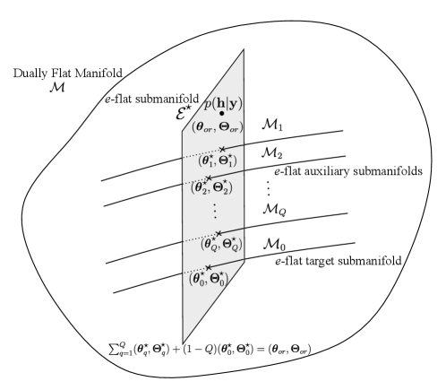
It means the original point, the target point and the auxiliary points are on a hyperplane in the affine coordinate system. This is called the ee-condition since it is a linear condition in the coordinate system 𝜽,𝚯\bm{\theta},\bm{\Theta} as shown in Fig. 1. Because of the split, the ee-condition always holds if

q=1Q(𝝀q,𝚲q)+(1Q)(𝝀0,𝚲0)=0.\displaystyle\sum_{q=1}^{Q}(\bm{\lambda}_{q},\bm{\Lambda}_{q})+(1-Q)(\bm{\lambda}_{0},\bm{\Lambda}_{0})=0. (24)

Thus, the above formula is also the ee-condition. The ee-condition makes sure the target point and auxiliary points are related to the original point, which is important to finally get an approximation of the mm-projection point.

III-D The mm-Condition and General Algorithm

The ee-condition only states the relation between the natural parameters of the original point, the auxiliary points, and the target point, but what we need is part of the expectation parameters of the original point. To obtain an approximation of the mm-projection point, we need another condition, i.e, the mm-condition.

The mm-condition is named because it is a linear condition in the dual affine coordinate system 𝝁,𝐌\bm{\mu},\mathbf{M}, and is given by

(𝝁q,𝐈𝐌q)=(𝝁0,𝐈𝐌0)qQ+.\displaystyle({\bm{\mu}}_{q}^{\star},\mathbf{I}\odot\mathbf{M}_{q}^{\star})=({\bm{\mu}}_{0}^{\star},\mathbf{I}\odot\mathbf{M}_{0}^{\star})\quad\forall q\in\mathbb{Z}_{Q}^{+}. (25)

From Section II-B, it means all the mm-projection points of the auxiliary points are the same and equal to the target point. By combining the mm-condition with the ee-condition, a good approximation of the mm-projection point on the target manifold of the original point can be obtained.

From (3a), the expectation parameters 𝝁q,𝐌q{\bm{\mu}}_{q},{\mathbf{M}}_{q} of auxiliary points can be obtained as

𝝁q\displaystyle{\bm{\mu}}_{q} =(𝚲q+𝐂q+𝚲c)1(𝝀q+𝐛q)\displaystyle=({\bm{\Lambda}}_{q}+\mathbf{C}_{q}+\bm{\Lambda}_{c})^{-1}({\bm{\lambda}}_{q}+\mathbf{b}_{q}) (26a)
𝐌q\displaystyle{\mathbf{M}}_{q} =𝝁q𝝁qH+(𝚲q+𝐂q+𝚲c)1.\displaystyle={\bm{\mu}}_{q}{\bm{\mu}}_{q}^{H}+({\bm{\Lambda}}_{q}+\mathbf{C}_{q}+\bm{\Lambda}_{c})^{-1}. (26b)

Then, the expectation parameters of the mm-projection points on the target manifold 0\mathcal{M}_{0} satisfies

\Hy@raisedlink\hyper@anchorstart\@IEEEtheHrefequation\Hy@raisedlink\hyper@anchorend𝝁q0\displaystyle{\Hy@raisedlink{\hyper@anchorstart{\@IEEEtheHrefequation}}\Hy@raisedlink{\hyper@anchorend}}{\bm{\mu}}_{q}^{0} =𝝁q\displaystyle={\bm{\mu}}_{q} (27a)
𝐈𝐌q0\displaystyle\mathbf{I}\odot{\mathbf{M}}_{q}^{0} =𝐈𝐌q\displaystyle=\mathbf{I}\odot{\mathbf{M}}_{q} (27b)

as shown in Section II-B, and further we have the covariance of the mm-projection 𝚺q0=𝐈𝚺q{\bm{\Sigma}}_{q}^{0}=\mathbf{I}\odot{\bm{\Sigma}}_{q}. The natural parameters of the mm-projection points can be obtained as

\Hy@raisedlink\hyper@anchorstart\@IEEEtheHrefequation\Hy@raisedlink\hyper@anchorend𝜽q0\displaystyle{\Hy@raisedlink{\hyper@anchorstart{\@IEEEtheHrefequation}}\Hy@raisedlink{\hyper@anchorend}}{\bm{\theta}}_{q}^{0} =𝚯q0(𝚲q+𝐂q+𝚲c)1(𝝀q+𝐛q)\displaystyle=-{\bm{\Theta}}_{q}^{0}({\bm{\Lambda}}_{q}+\mathbf{C}_{q}+\bm{\Lambda}_{c})^{-1}({\bm{\lambda}}_{q}+\mathbf{b}_{q}) (28a)
𝚯q0\displaystyle{\bm{\Theta}}_{q}^{0} =(𝐈(𝚲q+𝐂q+𝚲c)1)1.\displaystyle=-(\mathbf{I}\odot({\bm{\Lambda}}_{q}+\mathbf{C}_{q}+\bm{\Lambda}_{c})^{-1})^{-1}. (28b)

To make both the ee-condition and the mm-condition hold, the auxiliary points need to exchange beliefs. Define 𝝀q0{\bm{\lambda}}_{q}^{0} and 𝚲q0{\bm{\Lambda}}_{q}^{0} to make 𝜽q0=𝝀q0{\bm{\theta}}_{q}^{0}={\bm{\lambda}}_{q}^{0} and 𝚯q0=(𝚲q0+𝚲c){\bm{\Theta}}_{q}^{0}=-({\bm{\Lambda}}_{q}^{0}+\bm{\Lambda}_{c}) hold. The beliefs are defined as

\Hy@raisedlink\hyper@anchorstart\@IEEEtheHrefequation\Hy@raisedlink\hyper@anchorend𝝃q\displaystyle{\Hy@raisedlink{\hyper@anchorstart{\@IEEEtheHrefequation}}\Hy@raisedlink{\hyper@anchorend}}\bm{\xi}_{q} =𝝀q0𝝀q\displaystyle={\bm{\lambda}}_{q}^{0}-{\bm{\lambda}}_{q} (29a)
𝚵q\displaystyle\bm{\Xi}_{q} =𝚲q0𝚲q.\displaystyle={\bm{\Lambda}}_{q}^{0}-{\bm{\Lambda}}_{q}. (29b)

Then, the natural parameters of the mm-projection points can be expressed as

\Hy@raisedlink\hyper@anchorstart\@IEEEtheHrefequation\Hy@raisedlink\hyper@anchorend𝜽q0\displaystyle{\Hy@raisedlink{\hyper@anchorstart{\@IEEEtheHrefequation}}\Hy@raisedlink{\hyper@anchorend}}{\bm{\theta}}_{q}^{0} =𝝀q+𝝃q\displaystyle={\bm{\lambda}}_{q}+\bm{\xi}_{q} (30a)
𝚯q0\displaystyle{\bm{\Theta}}_{q}^{0} =(𝚲q+𝚵q+𝚲c).\displaystyle=-\left({\bm{\Lambda}}_{q}+\bm{\Xi}_{q}+\bm{\Lambda}_{c}\right). (30b)

By comparing them with the natural parameters of auxiliary point p(𝐡;𝜽q,𝚯q)p(\mathbf{h};{\bm{\theta}}_{q},{\bm{\Theta}}_{q}), it can be observed that 𝝃q\bm{\xi}_{q}, 𝚵q\bm{\Xi}_{q} are approximations of 𝐛q\mathbf{b}_{q}, 𝐂q\mathbf{C}_{q} in 𝜽q{\bm{\theta}}_{q} and 𝚯q{\bm{\Theta}}_{q}, respectively, where 𝚵q\bm{\Xi}_{q} is also diagonal.

After defining the beliefs, the iterative update of natural parameters of the target point and auxiliary points are constructed as

\Hy@raisedlink\hyper@anchorstart\@IEEEtheHrefequation\Hy@raisedlink\hyper@anchorend𝝀0t+1\displaystyle{\Hy@raisedlink{\hyper@anchorstart{\@IEEEtheHrefequation}}\Hy@raisedlink{\hyper@anchorend}}\bm{\lambda}_{0}^{t+1} =q𝝃qt\displaystyle=\sum_{q}\bm{\xi}_{q}^{t} (31a)
𝚲0t+1\displaystyle\bm{\Lambda}_{0}^{t+1} =q𝚵qt\displaystyle=\sum_{q}\bm{\Xi}_{q}^{t} (31b)

and

\Hy@raisedlink\hyper@anchorstart\@IEEEtheHrefequation\Hy@raisedlink\hyper@anchorend𝝀qt+1\displaystyle{\Hy@raisedlink{\hyper@anchorstart{\@IEEEtheHrefequation}}\Hy@raisedlink{\hyper@anchorend}}\bm{\lambda}_{q}^{t+1} =qq𝝃qt=𝝀0t+1𝝃qt\displaystyle=\sum_{q^{\prime}\neq q}\bm{\xi}_{q^{\prime}}^{t}=\bm{\lambda}_{0}^{t+1}-\bm{\xi}_{q}^{t} (32a)
𝚲qt+1\displaystyle\bm{\Lambda}_{q}^{t+1} =qq𝚵qt=𝚲0t+1𝚵qt.\displaystyle=\sum_{q^{\prime}\neq q}\bm{\Xi}_{q^{\prime}}^{t}=\bm{\Lambda}_{0}^{t+1}-\bm{\Xi}_{q}^{t}. (32b)

From the above two equations, it is observed that the ee-condition always holds. An information geometry based algorithm is obtained by iteratively calculating (28a), (29a), (31a) and (32a). When the algorithm converges, it is easy to obtain that

\Hy@raisedlink\hyper@anchorstart\@IEEEtheHrefequation\Hy@raisedlink\hyper@anchorend(𝜽q0)\displaystyle{\Hy@raisedlink{\hyper@anchorstart{\@IEEEtheHrefequation}}\Hy@raisedlink{\hyper@anchorend}}({\bm{\theta}}_{q}^{0})^{\star} =𝝀0\displaystyle={\bm{\lambda}}_{0}^{\star} (33a)
(𝚯q0)\displaystyle({\bm{\Theta}}_{q}^{0})^{\star} =(𝚲0+𝚲c)=𝚯0\displaystyle=-\left({\bm{\Lambda}}_{0}^{\star}+\bm{\Lambda}_{c}\right)={\bm{\Theta}}_{0}^{\star} (33b)

which means all the mm-projection points are equal to the target point, and is equivalent to the mm-condition. In conclusion, both the ee-condition and the mm-condition are satisfied when the algorithm converges.

Finally, the output of this algorithm is the mean and covariance of the target point

𝝁0\displaystyle{\bm{\mu}}_{0} =𝚯01𝜽0=𝚲01𝝀0\displaystyle=-{\bm{\Theta}}_{0}^{-1}{\bm{\theta}}_{0}={\bm{\Lambda}}_{0}^{-1}{\bm{\lambda}}_{0} (34a)
𝚺0\displaystyle{\bm{\Sigma}}_{0} =𝚯01=𝚲01.\displaystyle=-{\bm{\Theta}}_{0}^{-1}={\bm{\Lambda}}_{0}^{-1}. (34b)

It is regarded as the approximated mean and covariance of the marginal PDF corresponding to the original PDF. When the algorithm does not converge, damping can be introduced in the updating of beliefs to ensure the convergence of the algorithm without changing its equilibrium. Although the process of the mm-projection in (28a) still involves the matrix inversion, i.e., (𝚲q+𝐂q+𝚲c)1({\bm{\Lambda}}_{q}+\mathbf{C}_{q}+\bm{\Lambda}_{c})^{-1}, it can be implemented with low complexity by properly setting of 𝐂q\mathbf{C}_{q} since 𝚲q{\bm{\Lambda}}_{q} and 𝚲c\bm{\Lambda}_{c} are diagonal matrices. For example, in the IGA algorithm proposed in [11], the matrix 𝐂q\mathbf{C}_{q} is a rank-11 matrix.

III-E Geometrical Explanation

This iterative process and the stabilization point can be explained geometrically. Define the mm-flat manifold \mathcal{M}^{\star} and the ee-flat manifold \mathcal{E}^{\star} as

\displaystyle\mathcal{M}^{\star} ={p(𝐡;𝜽,𝚯)|(𝝁,𝐈𝐌)=(𝝁q,𝐈𝐌q)=(𝝁0,𝐈𝐌0),qQ+}\displaystyle=\left\{p(\mathbf{h};\bm{\theta},\bm{\Theta})|(\bm{\mu},\mathbf{I}\odot\mathbf{M})=(\bm{\mu}_{q}^{\star},\mathbf{I}\odot\mathbf{M}_{q}^{\star})=(\bm{\mu}_{0}^{\star},\mathbf{I}\odot\mathbf{M}_{0}^{\star}),\forall q\in\mathbb{Z}_{Q}^{+}\right\} (35a)
\displaystyle\mathcal{E}^{\star} ={p(𝐡;𝜽,𝚯)|(𝜽,𝚯)=q=1Qcq(𝜽q,𝚯q)+(1q=1Qcq)(𝜽0,𝚯0)}\displaystyle=\left\{p(\mathbf{h};\bm{\theta},\bm{\Theta})|(\bm{\theta},\bm{\Theta})=\sum_{q=1}^{Q}c_{q}({\bm{\theta}}_{q}^{\star},{\bm{\Theta}}_{q}^{\star})+(1-\sum_{q=1}^{Q}c_{q})({\bm{\theta}}_{0}^{\star},{\bm{\Theta}}_{0}^{\star})\right\} (35b)

where cqc_{q} are the positive coefficients. The geometric interpretation of the mm-condition is given by Fig. 2. The ee-flat auxiliary and target manifolds are perpendicular to the mm-flat manifold \mathcal{M}^{\star} under the metric induced by the KL divergence.
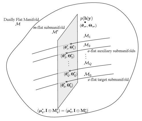
Refer to caption
Figure 2: mm-condition

From the ee-condition and the mm-condition shown in Figs. 1 and 2, it can be seen that when the algorithm converges, all the auxiliary points, the target points and the original points are also on the same ee-flat manifold \mathcal{E}^{\star}. Meanwhile, all the auxiliary points and the target point are on the same mm-flat manifold \mathcal{M}^{\star}. The mm-condition makes sure the mm-projection points of the auxiliary points and the target point are the same. The ee-condition relates the auxiliary points and the target point to the original point. By combining these two conditions, the original point is close to the manifold \mathcal{M}^{\star}. Theorem 11.8 of [17] proves that \mathcal{M}^{\star} contains the original point when the factor graph is acyclic, i.e., which means the exact mean of the original distribution is obtained. However, this property is not guaranteed when the factor graph is cyclic, which is the common case for the channel estimation problem. Fortunately, for the channel estimation problem, it is usually able to prove the mean 𝝁^0\hat{\bm{\mu}}_{0}^{\star} is equal to the mean 𝝁or\bm{\mu}_{or} when the algorithm converges as shown in [11].

IV IC-IGA for Massive MIMO Channel Estimation

In this section, an IC-IGA for massive MIMO channel estimation is proposed. First, a modified form equivalent to the MMSE estimation is given to define the auxiliary manifolds. Then, the framework of the information geometry approach is applied to derive this new IGA algorithm. Finally, the equilibrium and complexity analysis are provided.

IV-A Definition of Auxiliary Manifolds with Modified MMSE Form

In this subsection, we provide a new way of splitting the natural parameters based on a modified MMSE form. Then, the corresponding auxiliary manifolds are constructed.

To derive a new low-complexity IGA algorithm, we want to make each auxiliary manifold focus on the computation of one element of 𝐡\mathbf{h}. According to the framework of information geometry methods, the nn-th auxiliary PDF can be defined as

p(𝐡;𝜽n,𝚯n)=exp{𝐡H(𝝀n+𝐛n)+(𝝀nH+𝐛nH)𝐡𝐡H(𝚲n+𝐂n)𝐡ψn}\displaystyle p(\mathbf{h};{\bm{\theta}}_{n},{\bm{\Theta}}_{n})=\exp\{\mathbf{h}^{H}({\bm{\lambda}}_{n}+\mathbf{b}_{n})+({\bm{\lambda}}_{n}^{H}+\mathbf{b}_{n}^{H})\mathbf{h}-\mathbf{h}^{H}({\bm{\Lambda}}_{n}+\mathbf{C}_{n})\mathbf{h}-\psi_{n}\} (36)

where 𝜽n=𝝀n+𝐛n{\bm{\theta}}_{n}={\bm{\lambda}}_{n}+\mathbf{b}_{n} , 𝚯n=𝚲n+𝐂n{\bm{\Theta}}_{n}={\bm{\Lambda}}_{n}+\mathbf{C}_{n} and 𝚲c\bm{\Lambda}_{c} is set to be a zero matrix.

Let 𝐊=σz2𝐀H𝐀\mathbf{K}=\sigma_{z}^{-2}\mathbf{A}^{H}\mathbf{A}. To make the nn-th auxiliary PDF only compute the information of the nn-th element of 𝐡\mathbf{h}, a natural idea is to set 𝐂n\mathbf{C}_{n} and 𝐛n\mathbf{b}_{n} as

𝐏1n𝐂n𝐏1nH=(cn12𝐤¯nH12𝐤¯n𝟎),𝐏1n𝐛n=(1σz2𝐚nH𝐲𝟎)\displaystyle\mathbf{P}_{1n}\mathbf{C}_{n}\mathbf{P}_{1n}^{H}=\left(\begin{array}[]{cc}c_{n}&\frac{1}{2}\bar{\mathbf{k}}_{n}^{H}\\ \frac{1}{2}\bar{\mathbf{k}}_{n}&\mathbf{0}\end{array}\right),\qquad\mathbf{P}_{1n}\mathbf{b}_{n}=\left(\begin{array}[]{c}\frac{1}{\sigma_{z}^{2}}\mathbf{a}_{n}^{H}\mathbf{y}\\ \mathbf{0}\end{array}\right) (41)

where 𝐚n\mathbf{a}_{n} is the nn-th column of 𝐀\mathbf{A}, 𝐤¯n\bar{\mathbf{k}}_{n} is the vector obtained by deleting the nn-element knnk_{nn} from the nn-column of 𝐊\mathbf{K}, cn=σz2𝐚nH𝐚n+dn1c_{n}=\sigma_{z}^{-2}\mathbf{a}_{n}^{H}\mathbf{a}_{n}+d_{n}^{-1}, and 𝐏1nN×N\mathbf{P}_{1n}\in\mathbb{R}^{N\times N} is the ordering matrix obtained by extracting nn-th row of 𝐈N\mathbf{I}_{N} and put it in the first row. The matrix 𝐏1n\mathbf{P}_{1n} has the property that 𝐏1n𝐏1nH=𝐏1nH𝐏1n=𝐈N\mathbf{P}_{1n}\mathbf{P}_{1n}^{H}=\mathbf{P}_{1n}^{H}\mathbf{P}_{1n}=\mathbf{I}_{N}. By left-multiplying 𝐏1n\mathbf{P}_{1n} or right-multiplying 𝐏1nH\mathbf{P}_{1n}^{H}, one can extract the nn-th row or column of a given matrix and put it in the first row or column.

However, there is a flaw in this setup. The items associated with elements other than hnh_{n} in 𝐡\mathbf{h} are missing in the auxiliary function, and thus might not form a Gaussian-distributed PDF since 𝚲n+𝐂n{\bm{\Lambda}}_{n}+\mathbf{C}_{n} are not always positive semidefinite. To overcome this issue, we present the following theorem.

Theorem 1.

Let the matrices 𝐓\mathbf{T} and 𝚼\bm{\Upsilon} be defined as 𝐓=σz2𝐀H𝐀𝐈(σz2𝐀H𝐀)\mathbf{T}=\sigma_{z}^{-2}\mathbf{A}^{H}\mathbf{A}-\mathbf{I}\odot(\sigma_{z}^{-2}\mathbf{A}^{H}\mathbf{A}) and 𝚼=(𝐈(σz2𝐀H𝐀)+𝐃1)1\bm{\Upsilon}=\left(\mathbf{I}\odot(\sigma_{z}^{-2}\mathbf{A}^{H}\mathbf{A})+\mathbf{D}^{-1}\right)^{-1}. The estimator

𝐡^=(σz2𝐀H𝐀+𝐃1+𝐓+𝐓𝚼𝐓H)1(σz2𝐀H𝐲+𝐓𝚼σz2𝐀H𝐲)\displaystyle\hat{\mathbf{h}}=\left(\sigma_{z}^{-2}\mathbf{A}^{H}\mathbf{A}+\mathbf{D}^{-1}+\mathbf{T}+\mathbf{T}\bm{\Upsilon}\mathbf{T}^{H}\right)^{-1}\left(\sigma_{z}^{-2}\mathbf{A}^{H}\mathbf{y}+\mathbf{T}\bm{\Upsilon}\sigma_{z}^{-2}\mathbf{A}^{H}\mathbf{y}\right) (42)

is equivalent to the MMSE estimator.

Proof.

The proof is provided in Appendix A. ∎

Based on Theorem 1, we can use the following PDF

p(𝐡|𝐲)\displaystyle p(\mathbf{h}|\mathbf{y}) =exp{𝐡H(σz2𝐀H𝐲+𝐓𝚼σz2𝐀H𝐲)+(σz2𝐀H𝐲+𝐓𝚼σz2𝐀H𝐲)H𝐡\displaystyle=\exp\Big{\{}\mathbf{h}^{H}(\sigma_{z}^{-2}\mathbf{A}^{H}\mathbf{y}+\mathbf{T}\bm{\Upsilon}\sigma_{z}^{-2}\mathbf{A}^{H}\mathbf{y})+(\sigma_{z}^{-2}\mathbf{A}^{H}\mathbf{y}+\mathbf{T}\bm{\Upsilon}\sigma_{z}^{-2}\mathbf{A}^{H}\mathbf{y})^{H}\mathbf{h} (43)
𝐡H(σz2𝐀H𝐀+𝐃1+𝐓+𝐓𝚼𝐓H)1𝐡ψ~}\displaystyle\qquad\qquad-\mathbf{h}^{H}\left(\sigma_{z}^{-2}\mathbf{A}^{H}\mathbf{A}+\mathbf{D}^{-1}+\mathbf{T}+\mathbf{T}\bm{\Upsilon}\mathbf{T}^{H}\right)^{-1}\mathbf{h}-\tilde{\psi}\Big{\}}

to compute the original mean. With the modified MMSE form, we propose a new way of splitting natural parameter as

\Hy@raisedlink\hyper@anchorstart\@IEEEtheHrefequation\Hy@raisedlink\hyper@anchorend𝜽or=σz2𝐀H𝐲+𝐓𝚼σz2𝐀H𝐲=n=1N𝐛n\displaystyle{\Hy@raisedlink{\hyper@anchorstart{\@IEEEtheHrefequation}}\Hy@raisedlink{\hyper@anchorend}}\bm{\theta}_{or}=\sigma_{z}^{-2}\mathbf{A}^{H}\mathbf{y}+\mathbf{T}\bm{\Upsilon}\sigma_{z}^{-2}\mathbf{A}^{H}\mathbf{y}=\sum_{n=1}^{N}\mathbf{b}_{n} (44a)
𝚯or=(σz2𝐀H𝐀+𝐃1+𝐓+𝐓𝚼𝐓H)=(n=1N𝐂n)\displaystyle\bm{\Theta}_{or}=-(\sigma_{z}^{-2}\mathbf{A}^{H}\mathbf{A}+\mathbf{D}^{-1}+\mathbf{T}+\mathbf{T}\bm{\Upsilon}\mathbf{T}^{H})=-(\sum_{n=1}^{N}\mathbf{C}_{n}) (44b)

where 𝐛n\mathbf{b}_{n} and 𝐂n\mathbf{C}_{n} are defined as

𝐏1n𝐂n𝐏1nH=(cn𝐤¯nH𝐤¯n1cn𝐤¯n𝐤¯nH),𝐏1n𝐛n=(1σz2𝐚nH𝐲1σz21cn𝐤¯n𝐚nH𝐲).\displaystyle\mathbf{P}_{1n}\mathbf{C}_{n}\mathbf{P}_{1n}^{H}=\left(\begin{array}[]{cc}c_{n}&\bar{\mathbf{k}}_{n}^{H}\\ \bar{\mathbf{k}}_{n}&\frac{1}{c_{n}}\bar{\mathbf{k}}_{n}\bar{\mathbf{k}}_{n}^{H}\end{array}\right),\qquad\mathbf{P}_{1n}\mathbf{b}_{n}=\left(\begin{array}[]{c}\frac{1}{\sigma_{z}^{2}}\mathbf{a}_{n}^{H}\mathbf{y}\\ \frac{1}{\sigma_{z}^{2}}\frac{1}{c_{n}}\bar{\mathbf{k}}_{n}\mathbf{a}_{n}^{H}\mathbf{y}\end{array}\right). (49)

The natural parameter of the nn-th auxiliary PDF is defined as

\Hy@raisedlink\hyper@anchorstart\@IEEEtheHrefequation\Hy@raisedlink\hyper@anchorend𝜽n\displaystyle{\Hy@raisedlink{\hyper@anchorstart{\@IEEEtheHrefequation}}\Hy@raisedlink{\hyper@anchorend}}\bm{\theta}_{n} =𝝀n+𝐛n\displaystyle=\bm{\lambda}_{-n}+\mathbf{b}_{n} (50a)
𝚯n\displaystyle\bm{\Theta}_{n} =(𝚲n+𝐂n)\displaystyle=-(\bm{\Lambda}_{-n}+\mathbf{C}_{n}) (50b)

where 𝝀n,𝚲n\bm{\lambda}_{-n},\bm{\Lambda}_{-n} are given by

𝝀n=(λ1,,λn1,0,λn+1,,λN)T\displaystyle\bm{\lambda}_{-n}=(\lambda_{1},\cdots,\lambda_{n-1},0,\lambda_{n+1},\cdots,\lambda_{N})^{T} (51a)
𝚲n=diag(Λ1,,Λn1,0,Λn+1,,ΛN).\displaystyle\bm{\Lambda}_{-n}=\text{diag}(\Lambda_{1},\cdots,\Lambda_{n-1},0,\Lambda_{n+1},\cdots,\Lambda_{N}). (51b)

The subscript n{-n} instead of nn is used because we impose more constraints on 𝝀n,𝚲n\bm{\lambda}_{n},\bm{\Lambda}_{n}, and the nn-th element has been set to zero. The auxiliary PDF p(𝐡;𝜽n,𝚯n)p(\mathbf{h};\bm{\theta}_{n},\bm{\Theta}_{n}) can be constructed as

p(𝐡;𝜽n,𝚯n)=exp{𝐡H(𝝀n+𝐛n)+(𝝀nH+𝐛nH)𝐡𝐡H(𝚲n+𝐂n)𝐡ψn}.\displaystyle p(\mathbf{h};\bm{\theta}_{n},\bm{\Theta}_{n})=\exp\{\mathbf{h}^{H}(\bm{\lambda}_{-n}+\mathbf{b}_{n})+(\bm{\lambda}_{-n}^{H}+\mathbf{b}_{n}^{H})\mathbf{h}-\mathbf{h}^{H}(\bm{\Lambda}_{-n}+\mathbf{C}_{n})\mathbf{h}-\psi_{n}\}. (52)

and the corresponding auxiliary manifolds are n={p(𝐡;𝜽n,𝚯n)},nN+\mathcal{M}_{n}=\left\{p(\mathbf{h};\bm{\theta}_{n},\bm{\Theta}_{n})\right\},\forall n\in\mathbb{Z}_{N}^{+}.

The natural parameter of the target point is defined as 𝜽0=𝝀\bm{\theta}_{0}=\bm{\lambda}, 𝚯0=𝚲\bm{\Theta}_{0}=-\bm{\Lambda}, where

𝝀\displaystyle\bm{\lambda} =(λ1,λ2,,λN)T\displaystyle=(\lambda_{1},\lambda_{2},\cdots,\lambda_{N})^{T} (53a)
𝚲\displaystyle\bm{\Lambda} =diag(Λ1,Λ2,,ΛN).\displaystyle={\rm diag}(\Lambda_{1},\Lambda_{2},\cdots,\Lambda_{N}). (53b)

The target PDF becomes

p0(𝐡;𝜽0,𝚯0)=exp{𝐡H𝝀+𝝀H𝐡𝐡H𝚲𝐡ψ0}\displaystyle p_{0}(\mathbf{h};\bm{\theta}_{0},\bm{\Theta}_{0})=\exp\{\mathbf{h}^{H}\bm{\lambda}+\bm{\lambda}^{H}\mathbf{h}-\mathbf{h}^{H}\bm{\Lambda}\mathbf{h}-\psi_{0}\} (54)

and the target manifold is still 0={p(𝐡;𝜽0,𝚯0)}\mathcal{M}_{0}=\left\{p(\mathbf{h};\bm{\theta}_{0},\bm{\Theta}_{0})\right\}. It is easy to check the ee-condition always holds due to

n=1N(𝝀n,𝚲n)+(1N)(𝝀,𝚲)=0.\displaystyle\sum_{n=1}^{N}(\bm{\lambda}_{-n},\bm{\Lambda}_{-n})+(1-N)(\bm{\lambda},\bm{\Lambda})=0. (55)

IV-B Derivation of IC-IGA

After constructing the auxiliary manifolds, the estimation problem can be solved by applying the information geometry framework of section III. For convenience, we define 𝝀n,𝚲n\bm{\lambda}_{n},\bm{\Lambda}_{n} as

𝝀n=(λ1,,λn1,λn+1,,λN)T(N1)×1\displaystyle\bm{\lambda}_{n}=(\lambda_{1},\cdots,\lambda_{n-1},\lambda_{n+1},\cdots,\lambda_{N})^{T}\in\mathbb{C}^{(N-1)\times 1} (56a)
𝚲n=diag(Λ1,,Λn1,Λn+1,,ΛN)(N1)×(N1).\displaystyle\bm{\Lambda}_{n}=\text{diag}(\Lambda_{1},\cdots,\Lambda_{n-1},\Lambda_{n+1},\cdots,\Lambda_{N})\in\mathbb{C}^{(N-1)\times(N-1)}. (56b)

The following theorem gives the beliefs 𝝃n\bm{\xi}_{n}, 𝚵n\bm{\Xi}_{n} corresponding to the nn-th auxiliary point at the tt-th iteration.

Theorem 2.

Let the beliefs 𝛏n\bm{\xi}_{n}, 𝚵n\bm{\Xi}_{n} be defined as 𝛏n=𝛌n0𝛌n\bm{\xi}_{n}=\bm{\lambda}_{-n}^{0}-\bm{\lambda}_{-n} and 𝚵n=𝚲n0𝚲n\bm{\Xi}_{n}=\bm{\Lambda}_{-n}^{0}-\bm{\Lambda}_{-n}. Then, their elements are given by

[𝝃n]i={rnμn,i=n0,others\displaystyle[\bm{\xi}_{n}]_{i}=\begin{cases}r_{n}\mu_{n},\quad i=n\\ 0,\quad\text{others}\end{cases} (57a)
[𝚵n]ii={rn,i=n0,others\displaystyle{[\bm{\Xi}_{n}]}_{ii}=\begin{cases}r_{n},\quad i=n\\ 0,\quad\text{others}\end{cases} (57b)

where μn=1σz2cn1(𝐚nH𝐲𝐚nH𝐀𝚲1𝛌+𝐚nH𝐚nΛn1λn)\mu_{n}=\frac{1}{\sigma_{z}^{2}}c_{n}^{-1}\left(\mathbf{a}_{n}^{H}\mathbf{y}-\mathbf{a}_{n}^{H}\mathbf{A}\bm{\Lambda}^{-1}\bm{\lambda}+\mathbf{a}_{n}^{H}\mathbf{a}_{n}\Lambda_{n}^{-1}\lambda_{n}\right), rn=cn(1+en)1r_{n}=c_{n}(1+e_{n})^{-1}, and en=1cn𝐤¯nH𝚲n1𝐤¯ne_{n}=\frac{1}{c_{n}}\bar{\mathbf{k}}_{n}^{H}\bm{\Lambda}_{n}^{-1}\bar{\mathbf{k}}_{n}.

Proof.

The proof is provided in Appendix B. ∎

Before proceeding to the derivation of IC-IGA, we present more insights about Theorem 2. Let 𝐡¯n\bar{\mathbf{h}}_{n} and sns_{n} be defined as 𝐡¯n=(h1,,hn1,hn+1,,hN)T\bar{\mathbf{h}}_{n}=(h_{1},\cdots,h_{n-1},h_{n+1},\cdots,h_{N})^{T} and

sn\displaystyle s_{n} =1σz2𝐚nH𝐲𝐤¯nH𝐡¯n\displaystyle=\frac{1}{\sigma_{z}^{2}}\mathbf{a}_{n}^{H}\mathbf{y}-\bar{\mathbf{k}}_{n}^{H}\bar{\mathbf{h}}_{n} (58)

we have that

1Znexp{𝐡H𝐛n+𝐛nH𝐡𝐡H𝐂n𝐡}\displaystyle\frac{1}{Z_{n}}\exp\{\mathbf{h}^{H}\mathbf{b}_{n}+\mathbf{b}_{n}^{H}\mathbf{h}-\mathbf{h}^{H}\mathbf{C}_{n}\mathbf{h}\} =1Znexp{hnsn+snhnhncnhnsnsncn}\displaystyle=\frac{1}{Z_{n}}\exp\left\{h_{n}^{*}s_{n}+s_{n}^{*}h_{n}-h_{n}^{*}c_{n}h_{n}-\frac{s_{n}^{*}s_{n}}{c_{n}}\right\} (59)

where ZnZ_{n} is the normalization constant. It means this part of p(𝐡;𝜽n,𝚯n)p(\mathbf{h};\bm{\theta}_{n},\bm{\Theta}_{n}) can be viewed as a conditional PDF of hnh_{n} as p(hn|h1,,hn1,hn+1,,hN,𝐲)p(h_{n}|h_{1},\cdots,h_{n-1},h_{n+1},\cdots,h_{N},\mathbf{y}). Furthermore, the remain part of p(𝐡;𝜽n,𝚯n)p(\mathbf{h};\bm{\theta}_{n},\bm{\Theta}_{n}) can be viewed as

exp{𝐡H𝝀n+𝝀nH𝐡𝐡H𝚲n𝐡ψ}=p(h1|𝐲)p(hn1|𝐲)p(hn+1|𝐲)p(hN|𝐲).\displaystyle\exp\{\mathbf{h}^{H}\bm{\lambda}_{-n}+\bm{\lambda}_{-n}^{H}\mathbf{h}-\mathbf{h}^{H}\bm{\Lambda}_{-n}\mathbf{h}-\psi\}=p(h_{1}|\mathbf{y})\cdots p(h_{n-1}|\mathbf{y})p(h_{n+1}|\mathbf{y})\cdots p(h_{N}|\mathbf{y}). (60)

The corresponding PDF pn(𝐡;𝜽n,𝚯n)p_{n}(\mathbf{h};\bm{\theta}_{n},\bm{\Theta}_{n}) can be rewritten as

p(𝐡;𝜽n,𝚯n)\displaystyle\quad p(\mathbf{h};\bm{\theta}_{n},\bm{\Theta}_{n})
=p(hn|h1,,hn1,hn+1,,hN,𝐲)p(h1|𝐲)p(hn1|𝐲)p(hn+1|𝐲)p(hN|𝐲).\displaystyle=p(h_{n}|h_{1},\cdots,h_{n-1},h_{n+1},\cdots,h_{N},\mathbf{y})p(h_{1}|\mathbf{y})\cdots p(h_{n-1}|\mathbf{y})p(h_{n+1}|\mathbf{y})\cdots p(h_{N}|\mathbf{y}). (61)

Thus, the marginal PDF of other elements will be the same as that provided by 𝝀n,𝚲n\bm{\lambda}_{-n},\bm{\Lambda}_{-n}, and each auxiliary manifold only updates the marginal PDF of one element. This explains why the nn-th auxiliary manifold has a belief of 0 for the other elements as shown in Theorem 2.

From Theorem 2, the nn-th auxiliary manifold only computes the mean μn\mu_{n} and variance rn1r_{n}^{-1} of the nn-th element of 𝐡\mathbf{h}. The corresponding natural parameter is λn=rnμn,Λn=rn\lambda_{n}=r_{n}\mu_{n},\Lambda_{n}=r_{n}. In the computation, the mean and variance of the other elements are those of the other auxiliary manifolds in the previous iteration, which is consistent with the idea of interference cancellation (IC), and therefore this method is called IC-IGA.

After calculating the beliefs, the parameters 𝝀\bm{\lambda}, 𝚲\bm{\Lambda} and 𝝀n\bm{\lambda}_{-n}, 𝚲n\bm{\Lambda}_{-n} corresponding to the target and auxiliary points are updated based on (31a) and (32a). However, this update might cause the algorithm to diverge. By introducing damping, the convergence of the algorithm can be enhanced without changing its equilibrium. Let 0<α10<\alpha\leq 1 be the damping coefficient, the natural parameters λnt+1\lambda_{n}^{t+1} and Λnt+1\Lambda_{n}^{t+1} corresponding to the target and auxiliary points in 𝝀t+1\bm{\lambda}^{t+1}, 𝚲t+1\bm{\Lambda}^{t+1}, 𝝀nt+1\bm{\lambda}_{-n}^{t+1} and 𝚲nt+1\bm{\Lambda}_{-n}^{t+1} are updated as

\Hy@raisedlink\hyper@anchorstart\@IEEEtheHrefequation\Hy@raisedlink\hyper@anchorendλnt+1\displaystyle{\Hy@raisedlink{\hyper@anchorstart{\@IEEEtheHrefequation}}\Hy@raisedlink{\hyper@anchorend}}\lambda_{n}^{t+1} =αrnt+1μnt+1+(1α)λnt\displaystyle=\alpha r_{n}^{t+1}\mu_{n}^{t+1}+(1-\alpha)\lambda_{n}^{t} (62a)
Λnt+1\displaystyle\Lambda_{n}^{t+1} =αrnt+1+(1α)Λnt,\displaystyle=\alpha r_{n}^{t+1}+(1-\alpha)\Lambda_{n}^{t}, (62b)

where the computation of μnt\mu_{n}^{t} and rntr_{n}^{t} can be rewritten as

\Hy@raisedlink\hyper@anchorstart\@IEEEtheHrefequation\Hy@raisedlink\hyper@anchorendμnt+1\displaystyle{\Hy@raisedlink{\hyper@anchorstart{\@IEEEtheHrefequation}}\Hy@raisedlink{\hyper@anchorend}}\mu_{n}^{t+1} =1σz2cn1(𝐚nH𝐲𝐚nH𝐀(𝚲t)1𝝀t+𝐚nH𝐚n(Λnt)1λnt)\displaystyle=\frac{1}{\sigma_{z}^{2}}c_{n}^{-1}\left(\mathbf{a}_{n}^{H}\mathbf{y}-\mathbf{a}_{n}^{H}\mathbf{A}(\bm{\Lambda}^{t})^{-1}\bm{\lambda}^{t}+\mathbf{a}_{n}^{H}\mathbf{a}_{n}(\Lambda_{n}^{t})^{-1}\lambda_{n}^{t}\right) (63a)
rnt+1\displaystyle r_{n}^{t+1} =cn1+ent\displaystyle=\frac{c_{n}}{1+e_{n}^{t}} (63b)

where ent=1cn𝐤¯nH(𝚲nt)1𝐤¯ne_{n}^{t}=\frac{1}{c_{n}}\bar{\mathbf{k}}_{n}^{H}(\bm{\Lambda}_{n}^{t})^{-1}\bar{\mathbf{k}}_{n} and cn=1σz2𝐚nH𝐚n+dn1c_{n}=\frac{1}{\sigma_{z}^{2}}\mathbf{a}_{n}^{H}\mathbf{a}_{n}+d_{n}^{-1}. Besides, define the matrix 𝐋=(𝐀H𝐀)(𝐀H𝐀)\mathbf{L}=(\mathbf{A}^{H}\mathbf{A})\odot(\mathbf{A}^{H}\mathbf{A})^{*} and vector 𝐯=(Λ11,Λ21,,ΛN1)T\mathbf{v}=(\Lambda_{1}^{-1},\Lambda_{2}^{-1},\cdots,\Lambda_{N}^{-1})^{T}, then the computation of ente_{n}^{t} can be rewritten as

ent=1σz4cn1(𝐞nT𝐋𝐯t𝐚nH𝐚n(Λn1)t𝐚nH𝐚n)\displaystyle e_{n}^{t}=\frac{1}{\sigma_{z}^{4}}c_{n}^{-1}(\mathbf{e}_{n}^{T}\mathbf{L}\mathbf{v}^{t}-\mathbf{a}_{n}^{H}\mathbf{a}_{n}(\Lambda_{n}^{-1})^{t}\mathbf{a}_{n}^{H}\mathbf{a}_{n}) (64)

where 𝐞n=[𝐈N]:,n\mathbf{e}_{n}=[\mathbf{I}_{N}]_{:,n} is the vector where only the nn-th element is 11 and the rest are all 0s. The channel estimation IC-IGA is summarized as Algorithm 1.

Input: The received signal 𝐲\mathbf{y}, the a priori covariance 𝐃\mathbf{D} of 𝐡\mathbf{h} and the maximal iteration number TT.
Output: The approximated posterior mean 𝝁t\bm{\mu}^{t} and covariance (𝐫t)1(\mathbf{r}^{t})^{-1} of beam domain channel 𝐡\mathbf{h}.
1 Initialization t=0t=0, 𝝁t=𝟎\bm{\mu}^{t}=\mathbf{0}, 𝝀t=𝟎\bm{\lambda}^{t}=\mathbf{0}, 𝚲t=𝐈\bm{\Lambda}^{t}=\mathbf{I}, 𝐯t=𝟏\mathbf{v}^{t}=\mathbf{1}, calculate 𝐀H𝐲\mathbf{A}^{H}\mathbf{y}, 𝐀H𝐀\mathbf{A}^{H}\mathbf{A}, and 𝐋=(𝐀H𝐀)(𝐀H𝐀)\mathbf{L}=(\mathbf{A}^{H}\mathbf{A})\odot(\mathbf{A}^{H}\mathbf{A})^{*}.
2 while tTt\leq T do
3       Calculate the mm-projection of NN auxiliary points to the target manifold and the corresponding mean μnt+1\mu_{n}^{t+1} and covariance (rnt+1)1(r_{n}^{t+1})^{-1} as
μnt+1\displaystyle\mu_{n}^{t+1} =1σz2cn1(𝐚nH𝐲𝐚nH𝐀(𝚲t)1𝝀t+𝐚nH𝐚n(Λnt)1λnt)\displaystyle=\frac{1}{\sigma_{z}^{2}}c_{n}^{-1}\left(\mathbf{a}_{n}^{H}\mathbf{y}-\mathbf{a}_{n}^{H}\mathbf{A}(\bm{\Lambda}^{t})^{-1}\bm{\lambda}^{t}+\mathbf{a}_{n}^{H}\mathbf{a}_{n}(\Lambda_{n}^{t})^{-1}\lambda_{n}^{t}\right)
rnt+1\displaystyle r_{n}^{t+1} =cn1+ent\displaystyle=\frac{c_{n}}{1+e_{n}^{t}}
ent\displaystyle e_{n}^{t} =1σz4cn(𝐞nT𝐋𝐯t𝐚nH𝐚n(Λnt)1𝐚nH𝐚n).\displaystyle=\frac{1}{\sigma_{z}^{4}c_{n}}(\mathbf{e}_{n}^{T}\mathbf{L}\mathbf{v}^{t}-\mathbf{a}_{n}^{H}\mathbf{a}_{n}(\Lambda_{n}^{t})^{-1}\mathbf{a}_{n}^{H}\mathbf{a}_{n}).
Update the parameters of the target and auxiliary points as
\Hy@raisedlink\hyper@anchorstart\@IEEEtheHrefequation\Hy@raisedlink\hyper@anchorendλnt+1\displaystyle{\Hy@raisedlink{\hyper@anchorstart{\@IEEEtheHrefequation}}\Hy@raisedlink{\hyper@anchorend}}\lambda_{n}^{t+1} =αrnt+1μnt+1+(1α)λnt\displaystyle=\alpha r_{n}^{t+1}\mu_{n}^{t+1}+(1-\alpha)\lambda_{n}^{t} (65a)
Λnt+1\displaystyle\Lambda_{n}^{t+1} =αrnt+1+(1α)Λnt.\displaystyle=\alpha r_{n}^{t+1}+(1-\alpha)\Lambda_{n}^{t}.
t=t+1t=t+1.
4 end while
When the algorithm converges or t>Tt>T, output the posterior mean 𝝁t\bm{\mu}^{t} and covariance (𝐫t)1(\mathbf{r}^{t})^{-1} of 𝐡\mathbf{h}.
Algorithm 1 IC-IGA for channel estimation

IV-C Equilibrium and Complexity Analysis

In this subsection, we present analysis for the equilibrium, i.e., fixed point or limit point, and the complexity of the IC-IGA.

From (25) and (24), Algorithm 1 satisfies the following conditions at the equilibrium

𝝁=𝝁n,𝚺=𝐈𝚺n\displaystyle\bm{\mu}^{\star}=\bm{\mu}_{n}^{\star},\quad\bm{\Sigma}^{\star}=\mathbf{I}\odot\bm{\Sigma}_{n}^{\star} (66)
𝝀=1N1n=1N𝝀n,𝚲=1N1n=1N𝚲n\displaystyle\bm{\lambda}^{\star}=\frac{1}{N-1}\sum_{n=1}^{N}\bm{\lambda}_{-n}^{\star},\quad\bm{\Lambda}^{\star}=\frac{1}{N-1}\sum_{n=1}^{N}\bm{\Lambda}_{-n}^{\star} (67)

which leads to the following theorem.

Theorem 3.

At the equilibrium of IC-IGA, the mean 𝛍\bm{\mu}^{\star} of p(𝐡;𝛉0,𝚯0)p(\mathbf{h};\bm{\theta}_{0},\bm{\Theta}_{0}) is equal to the mean 𝛍MMSE\bm{\mu}_{\text{MMSE}} of the posterior distribution p(𝐡|𝐲)p(\mathbf{h}|\mathbf{y}).

Proof.

The proof is provided in Appendix C. ∎

We now analyze the complexity of the IC-IGA algorithm in terms of time complexity (or computational complexity) and space complexity. In each iteration, the time complexity is mainly in the multiplication of matrix 𝐋\mathbf{L} and vector 𝐯\mathbf{v}, where 𝐋N×N\mathbf{L}\in\mathbb{R}^{N\times N} and 𝐯N×1\mathbf{v}\in\mathbb{R}^{N\times 1}, so the complexity is 𝒪(N2)\mathcal{O}(N^{2}). Finally, the time complexity of this algorithm is 𝒪(TN2)\mathcal{O}(TN^{2}), and TT is the number of iterations. The free variables of this algorithm are NN-dimensional vectors 𝝁\bm{\mu}, 𝐫\mathbf{r}, 𝐞\mathbf{e}, 𝝀\bm{\lambda}, diag(𝚲)\text{diag}(\bm{\Lambda}), and the number of free variables is 5N5N, so the space complexity of this algorithm is 𝒪(N)\mathcal{O}(N). When TT is small, the complexity of this algorithm is lower compared with the time complexity of 𝒪(N3+N2M)\mathcal{O}(N^{3}+N^{2}M) and the space complexity of 𝒪(N3)\mathcal{O}(N^{3}) in the MMSE algorithm. In addition, compared with the time complexity of 𝒪(TMN)\mathcal{O}(TMN) and the space complexity of 𝒪(MN)\mathcal{O}(MN) in the existing IGA algorithm [11], the IC-IGA algorithm has a comparable time complexity and a lower space complexity when MM is comparable to NN. In practice, the channel dimension NN is often smaller than the received signal dimension MM due to the sparsity of the channel, and the IC-IGA algorithm has lower time complexity and space complexity compared to the IGA algorithm.

V IC-SIGA for Massive MIMO Channel Estimation with BSCM and ZC Sequences

In this section, an IC-SIGA with lower complexity is proposed based on the IC-IGA by directly constructing the iterative update of the mean. To further reduce the complexity of IC-SIGA in practical systems, a massive MIMO with UPA is considered. By using BSCM and ZC sequences, a practical receive model is then established, and finally, the complexity of IC-SIGA is reduced by FFT and sparsity of the beam domain channel.

V-A Derivation of IC-SIGA

In this subsection, we provide the derivation of IC-SIGA, which can further reduce the complexity of channel estimation.

From the previous section, it is clear that the time complexity of the IC-IGA algorithm is mainly in the multiplication 𝐋𝐯\mathbf{L}\mathbf{v}. This computation is related to the calculation of rnr_{n} and ene_{n}, which involves the computation of the corresponding variance of the mm-projection of each auxiliary point. In the following, we reconsider the computation of the mean corresponding to the mm-projection of each auxiliary point. From (63a) and 𝝁=(𝚲)1𝝀\bm{\mu}^{\star}=(\bm{\Lambda}^{\star})^{-1}\bm{\lambda}^{\star}, we can obtain

𝝁\displaystyle\bm{\mu}^{\star} =1σz2(𝐀H𝐲𝐀H𝐀𝝁+(𝐈𝐀H𝐀)𝝁)./𝐜\displaystyle=\frac{1}{\sigma_{z}^{2}}\left(\mathbf{A}^{H}\mathbf{y}-\mathbf{A}^{H}\mathbf{A}{\bm{\mu}}^{\star}+(\mathbf{I}\odot\mathbf{A}^{H}\mathbf{A}){\bm{\mu}}^{\star}\right)./\mathbf{c} (68)

where 𝐜=(c1,,cN)T\mathbf{c}=(c_{1},\cdots,c_{N})^{T}, cn=1σz2𝐚nH𝐚n+dn1c_{n}=\frac{1}{\sigma_{z}^{2}}\mathbf{a}_{n}^{H}\mathbf{a}_{n}+d_{n}^{-1}, and ././ denotes the element-by-element division of vectors. Equation (68) indicates that 𝝁\bm{\mu} can be updated without rnr_{n}, ene_{n}.

However, equation (68) might also not converge. Thus, we also need to introduce the damping coefficient 0<α10<\alpha\leq 1. Let 𝝁temp\bm{\mu}^{temp} be defined as

𝝁temp\displaystyle\bm{\mu}^{temp} =1σz2(𝐀H𝐲𝐀H𝐀𝝁t+(𝐈𝐀H𝐀)𝝁t)./𝐜\displaystyle=\frac{1}{\sigma_{z}^{2}}\left(\mathbf{A}^{H}\mathbf{y}-\mathbf{A}^{H}\mathbf{A}\bm{\mu}^{t}+(\mathbf{I}\odot\mathbf{A}^{H}\mathbf{A})\bm{\mu}^{t}\right)./\mathbf{c} (69)

where 𝝁t\bm{\mu}^{t} is the mean at the tt-th iteration. Then, the mean of the target point 𝝁t+1\bm{\mu}^{t+1} can be updated as

𝝁t+1=α𝝁temp+(1α)𝝁t.\displaystyle\bm{\mu}^{t+1}=\alpha\bm{\mu}^{temp}+(1-\alpha)\bm{\mu}^{t}. (70)

When the algorithm converges, output the mean of the target point 𝝁t\bm{\mu}^{t}. The IC-SIGA for channel estimation is summarized as Algorithm 2.

Input: The received signal 𝐲\mathbf{y}, the a priori covariance 𝐃\mathbf{D} of 𝐡\mathbf{h} and the maximal iteration number TT.
Output: The approximated posterior mean 𝝁t\bm{\mu}^{t} of beam domain channel 𝐡\mathbf{h}.
1 Initialization t=0t=0, 𝝁t=𝟎\bm{\mu}^{t}=\mathbf{0}, calculate 𝐀H𝐲\mathbf{A}^{H}\mathbf{y}, 𝐈𝐀H𝐀\mathbf{I}\odot\mathbf{A}^{H}\mathbf{A}.
2 while tTt\leq T do
3       Calculate the mm-projection of NN auxiliary points to the target manifold and the corresponding mean 𝝁temp\bm{\mu}^{temp} as
𝝁temp\displaystyle\bm{\mu}^{temp} =1σz2(𝐀H𝐲𝐀H𝐀𝝁t+(𝐈𝐀H𝐀)𝝁t)./𝐜.\displaystyle=\frac{1}{\sigma_{z}^{2}}\left(\mathbf{A}^{H}\mathbf{y}-\mathbf{A}^{H}\mathbf{A}\bm{\mu}^{t}+(\mathbf{I}\odot\mathbf{A}^{H}\mathbf{A})\bm{\mu}^{t}\right)./\mathbf{c}.
Update the mean of the target point as
𝝁t+1=α𝝁temp+(1α)𝝁t.\displaystyle\bm{\mu}^{t+1}=\alpha\bm{\mu}^{temp}+(1-\alpha)\bm{\mu}^{t}.
t=t+1t=t+1.
4 end while
When the algorithm converges or t>Tt>T, output the posterior mean 𝝁t\bm{\mu}^{t} of 𝐡\mathbf{h}.
Algorithm 2 IC-SIGA for channel estimation

For the equilibrium, we can have the following theorem by using similar methods as that in IC-IGA.

Theorem 4.

At the equilibrium of IC-SIGA, the mean 𝛍\bm{\mu}^{\star} is equal to the mean 𝛍MMSE\bm{\mu}_{\text{MMSE}} of the posterior distribution p(𝐡|𝐲)p(\mathbf{h}|\mathbf{y}).

Proof.

The proof is provided in Appendix D. ∎

V-B System Configuration and Channel Model of Massive MIMO

In this subsection, we consider a 3D massive MIMO system equipped with UPA. The system configuration and the BSCM are introduced to show the properties of the channel.

Consider a massive MIMO-OFDM system working in time division duplexing (TDD) mode. The antenna array at the BS is a UPA with Mr=MzMxM_{r}=M_{z}M_{x} antennas, where MzM_{z} and MxM_{x} are the numbers of vertical and horizontal antennas. All users are equipped with a single antenna. The carrier frequency is fcf_{c}, and the wavelength is λc\lambda_{c}. The vertical and horizontal antenna spacings dzd_{z} and dxd_{x} are both set to half wavelength. The number of OFDM subcarriers is NcN_{c}, of which MpM_{p} training subcarriers are used to transmit the uplink pilot signal. Let the set of training subcarrier indexes be defined as ={0,1,,Mp1}\mathcal{L}=\{\ell_{0},\ell_{1},\cdots,\ell_{M_{p}-1}\}. Let MgM_{g} and TsT_{s} be the length of the cyclic prefix (CP) and sampling interval, respectively. The subcarrier interval is Δf=1NcTs\Delta f=\frac{1}{N_{c}T_{s}} and the transmission bandwidth is B=MpΔfB=M_{p}\Delta f.

The directional cosines for the zz and xx axis are defined as ur=sinθru_{r}=\sin\theta_{r} and vr=cosθrsinϕrv_{r}=\cos\theta_{r}\sin\phi_{r}, where θr\theta_{r} and ϕr\phi_{r} are polar and azimuthal angles of arrival (AOA) at the BS. The space steering vector at the BS side is given by [7]

𝐯(ur,vr)=𝐯z(ur)𝐯x(vr)Mr×1\displaystyle\mathbf{v}(u_{r},v_{r})=\mathbf{v}_{z}(u_{r})\otimes\mathbf{v}_{x}(v_{r})\in\mathbb{C}^{M_{r}\times 1} (71)

where

𝐯z(u)=[1ej2πdzλcuej2π(Mz1)dzλcu]T\displaystyle\mathbf{v}_{z}(u)=[1~{}~{}e^{-j2\pi\tfrac{d_{z}}{\lambda_{c}}u}~{}~{}\cdots~{}~{}e^{-j2\pi\tfrac{(M_{z}-1)d_{z}}{\lambda_{c}}u}]^{T} (72)
𝐯x(v)=[1ej2πdxλcvej2π(Mx1)dxλcv]T.\displaystyle\mathbf{v}_{x}(v)=[1~{}~{}e^{-j2\pi\tfrac{d_{x}}{\lambda_{c}}v}~{}~{}\cdots~{}~{}e^{-j2\pi\tfrac{(M_{x}-1)d_{x}}{\lambda_{c}}v}]^{T}. (73)

Let uiu_{i} and vjv_{j} be sampled directional cosines, defined as

ui\displaystyle u_{i} =2(i1)NzNz,iNz+\displaystyle=\frac{2(i-1)-N_{z}}{N_{z}},~{}~{}i\in\mathbb{Z}_{N_{z}}^{+} (74)
vi\displaystyle v_{i} =2(j1)NxNx,jNx+.\displaystyle=\frac{2(j-1)-N_{x}}{N_{x}},~{}~{}j\in\mathbb{Z}_{N_{x}}^{+}. (75)

Based on the space steering vector, the matrix of sampled space steering vectors are defined by

𝐕=𝐕z𝐕xMr×Nr\displaystyle\mathbf{V}=\mathbf{V}_{z}\otimes\mathbf{V}_{x}\in\mathbb{C}^{M_{r}\times N_{r}} (76)

where

𝐕z\displaystyle\mathbf{V}_{z} =[𝐯z(u1)𝐯z(u2)𝐯z(uNz)]\displaystyle=[\mathbf{v}_{z}(u_{1})~{}~{}\mathbf{v}_{z}(u_{2})~{}~{}\cdots~{}~{}\mathbf{v}_{z}(u_{N_{z}})] (77a)
𝐕x\displaystyle\mathbf{V}_{x} =[𝐯x(v1)𝐯x(v2)𝐯x(vNx)].\displaystyle=[\mathbf{v}_{x}(v_{1})~{}~{}\mathbf{v}_{x}(v_{2})~{}~{}\cdots~{}~{}\mathbf{v}_{x}(v_{N_{x}})]. (77b)

The symbols Nz=FzMzN_{z}=F_{z}M_{z} and Nx=FxMxN_{x}=F_{x}M_{x} are the numbers of sampled horizontal and vertical cosines, where FzF_{z} and FxF_{x} are fine factors. The frequency steering vector is defined similarly as

𝐮(τ)=[1ej2πΔfτej2π(Mp1)Δfτ]T.\displaystyle\mathbf{u}(\tau)=\left[1~{}~{}e^{-j2\pi\Delta f\tau}~{}~{}\cdots~{}~{}e^{-j2\pi(M_{p}-1)\Delta f\tau}\right]^{T}. (78)

The matrix of sampled frequency steering vectors is then given by

𝐔=[𝐮(τ1)𝐮(τ2)𝐮(τNf)]Mp×Nf\displaystyle\mathbf{U}=[\mathbf{u}(\tau_{1})~{}~{}\mathbf{u}(\tau_{2})~{}~{}\cdots~{}~{}\mathbf{u}(\tau_{N_{f}})]\in\mathbb{C}^{M_{p}\times N_{f}} (79)

where Np=FpMpN_{p}=F_{p}M_{p} is the number of sampled delays, FpF_{p} is the fine factor, Nf=NpMgNcN_{f}=\left\lceil\frac{N_{p}M_{g}}{N_{c}}\right\rceil, and τr\tau_{r} are sampled delays, given by

τr\displaystyle\tau_{r} =r1NpΔf,rNf+.\displaystyle=\frac{r-1}{N_{p}\Delta f},~{}~{}r\in\mathbb{Z}_{N_{f}}^{+}. (80)

Finally, the space-frequency domain channel matrix of user kk can be expressed as [11, 7]

𝐆k=𝐕𝐇k𝐔TMr×Mp\displaystyle\mathbf{G}_{k}=\mathbf{V}\mathbf{H}_{k}\mathbf{U}^{T}\in\mathbb{C}^{M_{r}\times M_{p}} (81)

where 𝐇kNr×Nf\mathbf{H}_{k}\in\mathbb{C}^{N_{r}\times N_{f}} is the beam domain channel matrix. This model is called the BSCM. The beam-domain channel matrix 𝐇k\mathbf{H}_{k} has improved sparsity than the traditional beam-domain stochastic channel model based on the discrete Fourier transform (DFT) matrices [33]. The elements of 𝐇k\mathbf{H}_{k} are assumed to be independent and follow a complex Gaussian distribution with zero mean and different variances. The beam domain channel power matrix is defined as 𝛀k\bm{\Omega}_{k}, where [𝛀k]ij[\bm{\Omega}_{k}]_{ij} is the variance of [𝐇k]ij[\mathbf{H}_{k}]_{ij}. It is the statistical CSI and remains constant over a relatively longer period than the instantaneous CSI.

V-C Receive Model with BSCM and ZC Sequences

In this subsection, we describe a specific receive model in practical massive MIMO systems, which shows that 𝐀\mathbf{A} multiplying vector can be realized by FFT.

The object of channel estimation is to obtain the a posteriori information of the space-frequency channel 𝐆k\mathbf{G}_{k}, which can be calculated from the beam domain channel 𝐇k\mathbf{H}_{k} with deterministic matrices 𝐔\mathbf{U} and 𝐕\mathbf{V}. Thus, we focus on the estimation of 𝐇k\mathbf{H}_{k}. We use the pilot signal sequence in [34] as

𝐱k=𝐱~q𝐮(τ(p1)Nf+1)\displaystyle\mathbf{x}_{k}=\tilde{\mathbf{x}}_{q}\odot\mathbf{u}(\tau_{(p-1)N_{f}+1}) (82)

where 𝐱~qMp×1\tilde{\mathbf{x}}_{q}\in\mathbb{C}^{M_{p}\times 1} is the Zadoff-Chu (ZC) sequence defined as

[𝐱~q]l=ejπ(q1)l(l1)Nl,l=1,,Mp\displaystyle[\tilde{\mathbf{x}}_{q}]_{l}=e^{-j\frac{\pi(q-1)l(l-1)}{N_{l}}},\ l=1,\cdots,M_{p} (83)

where NlN_{l} is the largest prime number satisfying Nl<MpN_{l}<M_{p}, q=(k1)/P+1q=\lfloor(k-1)/P\rfloor+1 and p=((k1)modP)+1p=\left((k-1)\bmod P\right)+1 denote the root coefficient and cyclic shift, Q=K/PQ=\lceil K/P\rceil is the number of roots, PP is the number of UEs of each root, and τ(p1)Nf+1\tau_{(p-1)N_{f}+1} is the sampled delay defined in (80).

Let 𝐗k=diag(𝐱k)Mp×Mp\mathbf{X}_{k}=\text{diag}(\mathbf{x}_{k})\in\mathbb{C}^{M_{p}\times M_{p}} be the pilot matrix. The received pilot signal matrix 𝐘tMr×Mp\mathbf{Y}_{t}\in\mathbb{C}^{M_{r}\times M_{p}} at the tt-th OFDM symbol is expressed as

𝐘t=k=1K𝐆k,t𝐗k+𝐙t\displaystyle\mathbf{Y}_{t}=\sum\limits_{k=1}^{K}\mathbf{G}_{k,t}\mathbf{X}_{k}+\mathbf{Z}_{t} (84)

where the noise matrix 𝐙t\mathbf{Z}_{t} consists of i.i.d. elements with zero mean and variance σz2\sigma_{z}^{2}.

For convenience, the subscript tt of the OFDM symbol is omitted hereafter. Substituting (81) and (82) into (84), we have

𝐘\displaystyle\mathbf{Y} =q=1Q𝐕(p=1P𝐇q,p𝐔Tdiag(𝐮(τ(p1)Nf+1)))𝐗~q+𝐙\displaystyle=\sum\limits_{q=1}^{Q}\mathbf{V}\left(\sum\limits_{p=1}^{P}\mathbf{H}_{q,p}\mathbf{U}^{T}\text{diag}\left(\mathbf{u}(\tau_{(p-1)N_{f}+1})\right)\right)\tilde{\mathbf{X}}_{q}+\mathbf{Z} (85)

where 𝐗~q=diag(𝐱~q)\tilde{\mathbf{X}}_{q}=\text{diag}\left(\tilde{\mathbf{x}}_{q}\right). Let 𝐅Np\mathbf{F}_{N_{p}} be an NpN_{p}-dimensional DFT matrix and define the partial DFT matrix 𝐔F=[𝐮(τ1),,𝐮(τNp)]Mp×Np\mathbf{U}_{F}=[\mathbf{u}(\tau_{1}),\cdots,\mathbf{u}(\tau_{N_{p}})]\in\mathbb{C}^{M_{p}\times N_{p}}. We then have 𝐔=𝐔F𝐈Np,Nf\mathbf{U}=\mathbf{U}_{F}\mathbf{I}_{N_{p},N_{f}} and 𝐔F=𝐈Mp,Np𝐅Np\mathbf{U}_{F}=\mathbf{I}_{M_{p},N_{p}}\mathbf{F}_{N_{p}}.

In (85), 𝐔Tdiag(𝐮(τ(p1)Nf+1))\mathbf{U}^{T}\text{diag}\left(\mathbf{u}(\tau_{(p-1)N_{f}+1})\right) can be calculated as

𝐔Tdiag(𝐮(τ(p1)Nf+1))\displaystyle\mathbf{U}^{T}\text{diag}\left(\mathbf{u}(\tau_{(p-1)N_{f}+1})\right) =𝐈Nf,Np𝚷Np(p1)Nf𝐔FT\displaystyle=\mathbf{I}_{N_{f},N_{p}}\bm{\Pi}_{N_{p}}^{(p-1)N_{f}}\mathbf{U}_{F}^{T} (86)

where

𝚷Nn=(𝟎𝐈Nn𝐈n𝟎)\displaystyle\bm{\Pi}_{N}^{n}=\left(\begin{array}[]{cc}\mathbf{0}&\mathbf{I}_{N-n}\\ \mathbf{I}_{n}&\mathbf{0}\end{array}\right) (89)

is the permutation matrix. Then, (85) can be reexpressed as

𝐘\displaystyle\mathbf{Y} =q=1Q𝐕(p=1P𝐇q,p𝐈Nf,Np𝚷Np(p1)Nf)𝐔FT𝐗~q+𝐙.\displaystyle=\sum\limits_{q=1}^{Q}\mathbf{V}(\sum\limits_{p=1}^{P}\mathbf{H}_{q,p}\mathbf{I}_{N_{f},N_{p}}\bm{\Pi}_{N_{p}}^{(p-1)N_{f}})\mathbf{U}_{F}^{T}\tilde{\mathbf{X}}_{q}+\mathbf{Z}. (90)

When PNp/NfP\leq\lfloor N_{p}/N_{f}\rfloor, we can avoid mutual aliasing of UEs with the same root and define

𝐇~q\displaystyle\tilde{\mathbf{H}}_{q} =[𝐇q,1,,𝐇q,P,𝟎Nr,NpPNf]Nr×Np.\displaystyle=\left[\mathbf{H}_{q,1},\cdots,\mathbf{H}_{q,P},\mathbf{0}_{N_{r},N_{p}-PN_{f}}\right]\in\mathbb{C}^{N_{r}\times N_{p}}. (91)

Finally, the uplink received signal model is given as

𝐘=𝐕𝐇𝐏+𝐙\displaystyle\mathbf{Y}=\mathbf{V}\mathbf{H}\mathbf{P}+\mathbf{Z} (92)

where

𝐇\displaystyle\mathbf{H} =[𝐇~1𝐇~2𝐇~Q]\displaystyle=[\tilde{\mathbf{H}}_{1}~{}~{}\tilde{\mathbf{H}}_{2}~{}~{}\cdots~{}~{}\tilde{\mathbf{H}}_{Q}] (93)
𝐏\displaystyle\mathbf{P} =[𝐗~1𝐔F𝐗~2𝐔F𝐗~Q𝐔F]T.\displaystyle=[\tilde{\mathbf{X}}_{1}\mathbf{U}_{F}~{}~{}\tilde{\mathbf{X}}_{2}\mathbf{U}_{F}~{}~{}\cdots~{}~{}\tilde{\mathbf{X}}_{Q}\mathbf{U}_{F}]^{T}. (94)

By vectorizing (92), the received signal model in vector form is

𝐲=𝐀~𝐡~+𝐳\displaystyle\mathbf{y}=\tilde{\mathbf{A}}\tilde{\mathbf{h}}+\mathbf{z} (95)

where 𝐲=vec(𝐘)M×1\mathbf{y}=\text{vec}(\mathbf{Y})\in\mathbb{C}^{M\times 1}, 𝐀~=𝐏T𝐕M×N~\tilde{\mathbf{A}}=\mathbf{P}^{T}\otimes\mathbf{V}\in\mathbb{C}^{M\times\tilde{N}}, 𝐡~=vec(𝐇)N~×1\tilde{\mathbf{h}}=\text{vec}(\mathbf{H})\in\mathbb{C}^{\tilde{N}\times 1}, 𝐳=vec(𝐙)𝒞𝒩(𝟎,σz2𝐈)\mathbf{z}=\text{vec}(\mathbf{Z})\sim\mathcal{CN}(\mathbf{0},\sigma_{z}^{2}\mathbf{I}), M=MrMpM=M_{r}M_{p}, and N~=QNpNr\tilde{N}=QN_{p}N_{r}. Since the beam domain channels are sparse, we can obtain a low dimensional 𝐡=𝐄~𝐡N×1\mathbf{h}=\tilde{\mathbf{E}}\mathbf{h}\in\mathbb{C}^{N\times 1} from 𝐡~\tilde{\mathbf{h}} by removing the elements with zero variance, where 𝐄~\tilde{\mathbf{E}} is the extraction matrix. Then, the general received signal model 𝐲=𝐀𝐡+𝐳\mathbf{y}={\mathbf{A}}{\mathbf{h}}+\mathbf{z} in (13) can be obtained, where 𝐀M×N\mathbf{A}\in\mathbb{C}^{M\times N} is the matrix obtained by removing corresponding columns of 𝐀~\tilde{\mathbf{A}}, and 𝐃\mathbf{D} can be obtained from 𝛀k\bm{\Omega}_{k} of all users.

V-D Complexity Analysis

The time complexity of the IC-SIGA algorithm is mainly in the multiplication 𝐀H𝐛\mathbf{A}^{H}\mathbf{b} and 𝐀𝐬\mathbf{A}\mathbf{s}, where 𝐬\mathbf{s} and 𝐛\mathbf{b} are two arbitrary vectors. In the following, we analyze the fast implementation method and complexity of the operation 𝐀H𝐛\mathbf{A}^{H}\mathbf{b}. The computation of 𝐀𝐬\mathbf{A}\mathbf{s} can be implemented similarly.

The computation of 𝐀H𝐛\mathbf{A}^{H}\mathbf{b} can be written as 𝐀H𝐛=𝐀~H𝐛~\mathbf{A}^{H}\mathbf{b}=\tilde{\mathbf{A}}^{H}\tilde{\mathbf{b}}. From 𝐀~=𝐏T𝐕\tilde{\mathbf{A}}=\mathbf{P}^{T}\otimes\mathbf{V}, the vector 𝐀~H𝐛~\tilde{\mathbf{A}}^{H}\tilde{\mathbf{b}} can be transformed into a matrix as 𝐀~H𝐛~=vec(𝐕H𝐁𝐏H)\tilde{\mathbf{A}}^{H}\tilde{\mathbf{b}}=\text{vec}(\mathbf{V}^{H}\mathbf{B}\mathbf{P}^{H}), where 𝐁Mr×Mp\mathbf{B}\in\mathbb{C}^{M_{r}\times M_{p}}, vec(𝐁)=𝐛~\text{vec}(\mathbf{B})=\tilde{\mathbf{b}}. Substituting the expression (94) for 𝐏\mathbf{P} yields 𝐁𝐏H=𝐁(𝐗~1𝐈Mp,Np𝐅Np,,𝐗~Q𝐈Mp,Np𝐅Np)\mathbf{B}\mathbf{P}^{H}=\mathbf{B}(\tilde{\mathbf{X}}_{1}^{*}\mathbf{I}_{M_{p},N_{p}}\mathbf{F}_{N_{p}}^{*},\cdots,\tilde{\mathbf{X}}_{Q}^{*}\mathbf{I}_{M_{p},N_{p}}\mathbf{F}_{N_{p}}^{*}). Define 𝐁~q=[𝐁𝐗~q,𝟎Mp,NpMp]Mr×Np\tilde{\mathbf{B}}_{q}=[\mathbf{B}\tilde{\mathbf{X}}_{q}^{*},\mathbf{0}_{M_{p},N_{p}-M_{p}}]\in\mathbb{C}^{M_{r}\times N_{p}}, then 𝐁𝐗~q𝐈Mp,Np𝐅Np=𝐁~q𝐅Np\mathbf{B}\tilde{\mathbf{X}}_{q}^{*}\mathbf{I}_{M_{p},N_{p}}\mathbf{F}_{N_{p}}^{*}=\tilde{\mathbf{B}}_{q}\mathbf{F}_{N_{p}}^{*}, where 𝐁~q𝐅Np\tilde{\mathbf{B}}_{q}\mathbf{F}_{N_{p}}^{*} can be realized by FFT. Since 𝐗q\mathbf{X}_{q}^{*} is a diagonal matrix, the complexity of 𝐁𝐗q\mathbf{B}\mathbf{X}_{q}^{*} is negligible. Thus, the time complexity of 𝐁𝐏H\mathbf{B}\mathbf{P}^{H} is 𝒪(QMrNplog2Np)\mathcal{O}(QM_{r}N_{p}\log_{2}N_{p}).

From (77a) we have 𝐕=(𝐈Mz,Nz𝐈Mx,Nx)(𝐅Nz𝐅Nx).\mathbf{V}=(\mathbf{I}_{M_{z},N_{z}}\otimes\mathbf{I}_{M_{x},N_{x}})(\mathbf{F}_{N_{z}}\otimes\mathbf{F}_{N_{x}}). Then, 𝐕H(𝐁𝐏H)\mathbf{V}^{H}(\mathbf{B}\mathbf{P}^{H}) can be realized by FFT with a time complexity of 𝒪(QNpNrlog2Nr)\mathcal{O}(QN_{p}N_{r}\log_{2}N_{r}). In summary, the time complexity of IC-SIGA is 𝒪(TQ(MrNplog2Np+NpNrlog2Nr))\mathcal{O}\left(TQ(M_{r}N_{p}\log_{2}N_{p}+N_{p}N_{r}\log_{2}N_{r})\right) b where TT is the iteration number.

Then, we analyze the space complexity. In IC-SIGA, the free variables are NN-dimensional vectors 𝝁temp\bm{\mu}^{temp}, 𝝁t\bm{\mu}^{t}, and the number of free variables is 2N2N. Therefore, the space complexity of IC-SIGA is 𝒪(N)\mathcal{O}(N).

VI Simulation Results

TABLE I: Parameter Setting of the QuaDRiGa
Parameter Value
Number of BS antenna Mr=Mz×MxM_{r}=M_{z}\times M_{x} 128 == 8 ×\times 16
UT number KK 12, 24
Center frequency fcf_{c} 4.8GHz
Number of subcarriers NcN_{c} 2048
Subcarrier spacing Δf\Delta f 30kHz
Number of training subcarriers MpM_{p} 120
CP length MgM_{g} 144
Refer to caption
Figure 3: The layout of the massive MIMO-OFDM system.

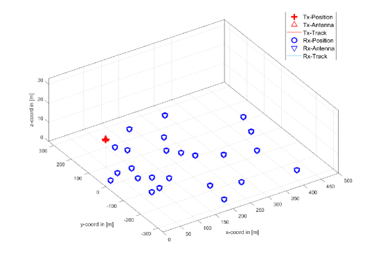
In this section, we provide simulation results to show the performance of the proposed IC-IGA and IC-SIGA for MIMO-OFDM channel estimation. We use the widely used QuaDRiGa channel model. The simulation scenario is set to “3GPP_\_38.901_\_UMa_\_NLOS”. The main parameters for the simulations are summarized in Table I. The layout of this massive MIMO-OFDM system is plotted in Fig. 3, where the location of the BS is at (0,0,25)(0,0,25), and the users are randomly generated in a 120120^{\circ} sector with radius r=500r=500m around (0,0,0)(0,0,0) at 1.51.5m height. The channel is normalized as 𝔼{𝐆kF2}=MrMp\mathbb{E}\{\|\mathbf{G}_{k}\|_{F}^{2}\}=M_{r}M_{p}. Fine factors are set as Fz=Fx=Fp=2F_{z}=F_{x}=F_{p}=2. The SNR is set as SNR =1/σz2=1/\sigma_{z}^{2}. We use the algorithm proposed in [7] to obtain the beam domain channel power matrices 𝛀k,k\bm{\Omega}_{k},\forall k. The normalized mean-squared error (NMSE) is used as the performance metric for the channel estimation, and is defined as

NMSE=1KNsamk=1Kn=1Nsam𝐆¯k,n𝐆k,nF2𝐆k,nF2\displaystyle\text{NMSE}=\frac{1}{KN_{sam}}\sum\limits_{k=1}^{K}\sum\limits_{n=1}^{N_{sam}}\frac{\|\bar{\mathbf{G}}_{k,n}-\mathbf{G}_{k,n}\|_{F}^{2}}{\|\mathbf{G}_{k,n}\|_{F}^{2}} (96)

where NsamN_{sam} is the number of the received pilot signals, 𝐆k,n\mathbf{G}_{k,n} is the exact space-frequency domain channel matrix, and 𝐆¯k,n\bar{\mathbf{G}}_{k,n} is the estimated space-frequency domain channel matrix. We set Nsam=200N_{sam}=200 in our simulations.

TABLE II: Complexities of algorithms
Algorithm Time Complexity Space Complexity
IC-IGA 𝒪(TN2)\mathcal{O}(TN^{2}) 𝒪(N)\mathcal{O}(N)
IC-SIGA 𝒪(TQ(MrNplog2Np+NpNrlog2Nr))\mathcal{O}\left(TQ(M_{r}N_{p}\log_{2}N_{p}+N_{p}N_{r}\log_{2}N_{r})\right) 𝒪(N)\mathcal{O}(N)
IGA 𝒪(TMN)\mathcal{O}(TMN) 𝒪(MN)\mathcal{O}(MN)
MMSE 𝒪(N3+N2M)\mathcal{O}(N^{3}+N^{2}M) 𝒪(N3)\mathcal{O}(N^{3})
Refer to caption
Figure 4: Time Complexity.
Refer to caption
Figure 5: Space Complexity.

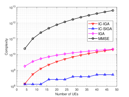
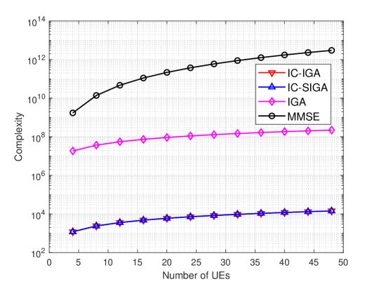
First, we present simulation results to show the complexity performance of different algorithms. The complexity of the IC-IGA, IC-SIGA, IGA, and MMSE algorithms is summarized in Table II. The time complexity and space complexity of the above four algorithms are presented in Figs. 4 and 5 for comparison, where the number of iterations is T=100T=100, the number of pilot roots is Q=K/PQ=\lceil K/P\rceil, and simulation parameters are configured as in Table I. From the figure, it can be found that the order of the time complexities of these algorithms is IC-SIGA<<IC-IGA<<IGA<<MMSE, and the order of the space complexities of these algorithms is IC-SIGA==IC-IGA<<IGA<<MMSE. Meanwhile, the time complexity of IC-SIGA algorithm is the same for the same number of pilot roots. The time complexity of IC-IGA is much less than the MMSE algorithm and also less than the IGA, whereas the space complexity of IC-IGA is much less than the IGA and MMSE algorithm. The time complexity of IC-SIGA is much less than other algorithms, and the space complexity of IC-SIGA is much less than that of the IGA and the MMSE algorithm.

Refer to caption
Figure 6: NMSE performance of IC-IGA and IC-SIGA compared with MMSE

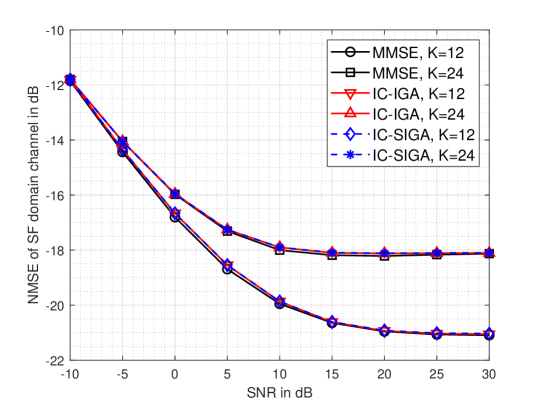
Fig. 6 shows the NMSE performance of IC-IGA and IC-SIGA channel estimation compared with IGA and MMSE. The user number is set to be K=12K=12 and K=24K=24. The iteration numbers of IC-IGA and IC-SIGA are set as 100. The damping coefficients of IC-IGA and IC-SIGA are αIC-IGA=0.45\alpha_{\text{IC-IGA}}=0.45 and αIC-SIGA=0.25\alpha_{\text{IC-SIGA}}=0.25, respectively. From the figure, it can be seen that both IC-IGA and IC-SIGA can obtain almost the same performance as MMSE for all SNR scenarios with two numbers of users. In addition, the performance using orthogonal pilots is more accurate, which is because the non-orthogonal pilots introduce interference from the pilots of users with other roots.

Refer to caption
Figure 7: Convergence performance of IC-IGA and IC-SIGA at SNR=10dB

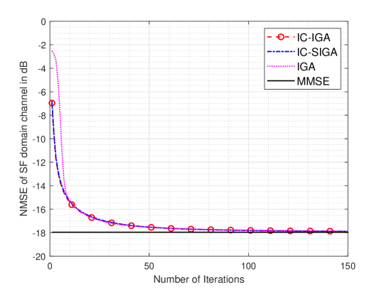
Fig. 7 plots the convergence performance of the IC-IGA and IC-SIGA for K=24K=24 at SNR=1010dB. The results of the MMSE estimation and the IGA in [11] are given for comparison. The damping coefficients of IGA, IC-IGA and IC-SIGA are αIGA=0.05\alpha_{\text{IGA}}=0.05, αIC-IGA=0.45\alpha_{\text{IC-IGA}}=0.45 and αIC-SIGA=0.25\alpha_{\text{IC-SIGA}}=0.25. As shown in the figure, the NMSE performance of IC-IGA and IC-SIGA can converge close to that of the MMSE estimation, which is consistent with Theorems 3 and 4. Furthermore, the NMSE of the IC-IGA decreases rapidly at the beginning, but the convergence speeds of the three algorithms, IC-IGA, IC-SIGA, and IGA, are nearly the same after about 1010 iterations.

Refer to caption
Figure 8: Convergence performance of IC-IGA
Refer to caption
Figure 9: Convergence performance of IC-SIGA

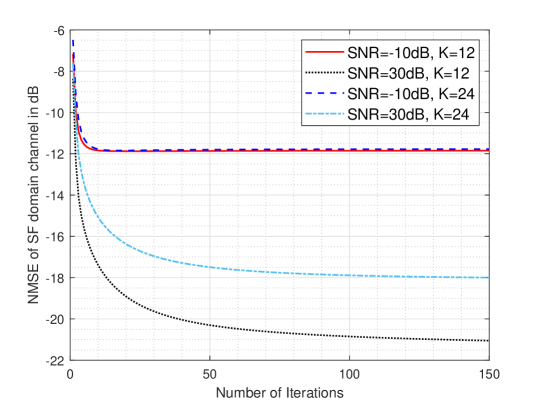
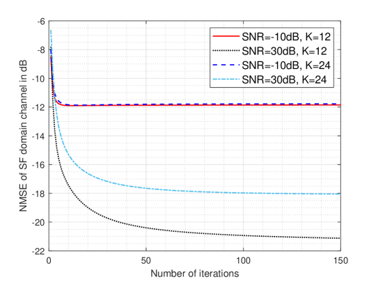
Fig. 8 and Fig. 9 show the convergence performance curves of IC-IGA and IC-SIGA for the orthogonal pilots case (K=12K=12) and non-orthogonal pilots (K=24K=24) case at different SNRs. The SNRs under consideration are low SNR scenarios SNR=10dB\text{SNR}=-10\text{dB} and high SNR scenarios where SNR=30dB\text{SNR}=30\text{dB}. From the figure, it can be seen that IC-IGA and IC-SIGA can approach convergence within 1010 iterations in the low SNR scenario, and 6060 iterations in the high SNR scenario.

VII Conclusion

In this paper, manifolds of complex Gaussian distributions are illustrated under information geometry theory, and a unified information geometry framework for channel estimation is described. To obtain an interference cancellation style algorithm, a modified MMSE form that has the same mean as the original MMSE estimator is constructed. Based on the unified framework and the modified form, the IC-IGA is then proposed for massive MIMO. The form of IC-IGA is simpler than IGA. Then, IC-SIGA is proposed to further reduce the complexity. The equilibria and complexities of the algorithms are analyzed. Simulation results show that the proposed methods can obtain similar performance to the IGA algorithm with fewer iterations and lower complexity.

Appendix A Proof of Theorem 1

It is easy to verify that 𝐈+𝐓𝚼\mathbf{I}+\mathbf{T}\bm{\Upsilon} is invertible. Simultaneously multiplying 𝐈+𝐓𝚼\mathbf{I}+\mathbf{T}\bm{\Upsilon} inside and outside the matrix inversion in the MMSE estimator yields

(σz2𝐀H𝐀+𝐃1)1(σz2𝐀H𝐲)\displaystyle\quad\left(\sigma_{z}^{-2}\mathbf{A}^{H}\mathbf{A}+\mathbf{D}^{-1}\right)^{-1}\left(\sigma_{z}^{-2}\mathbf{A}^{H}\mathbf{y}\right)
=((𝐈+𝐓𝚼)(σz2𝐀H𝐀+𝐃1))1(𝐈+𝐓𝚼)(σz2𝐀H𝐲)\displaystyle=\left((\mathbf{I}+\mathbf{T}\bm{\Upsilon})(\sigma_{z}^{-2}\mathbf{A}^{H}\mathbf{A}+\mathbf{D}^{-1})\right)^{-1}(\mathbf{I}+\mathbf{T}\bm{\Upsilon})\left(\sigma_{z}^{-2}\mathbf{A}^{H}\mathbf{y}\right)
=(σz2𝐀H𝐀+𝐃1+𝐓𝚼σz2𝐀H𝐀+𝐓𝚼𝐃1)1(σz2𝐀H𝐲+𝐓𝚼σz2𝐀H𝐲).\displaystyle=\left(\sigma_{z}^{-2}\mathbf{A}^{H}\mathbf{A}+\mathbf{D}^{-1}+\mathbf{T}\bm{\Upsilon}\sigma_{z}^{-2}\mathbf{A}^{H}\mathbf{A}+\mathbf{T}\bm{\Upsilon}\mathbf{D}^{-1}\right)^{-1}\left(\sigma_{z}^{-2}\mathbf{A}^{H}\mathbf{y}+\mathbf{T}\bm{\Upsilon}\sigma_{z}^{-2}\mathbf{A}^{H}\mathbf{y}\right). (97)

By using σz2𝐀H𝐀=𝐓H+𝐈(σz2𝐀H𝐀)\sigma_{z}^{-2}\mathbf{A}^{H}\mathbf{A}=\mathbf{T}^{H}+\mathbf{I}\odot(\sigma_{z}^{-2}\mathbf{A}^{H}\mathbf{A}), it follows that

(σz2𝐀H𝐀+𝐃1)1(σz2𝐀H𝐲)\displaystyle\quad\left(\sigma_{z}^{-2}\mathbf{A}^{H}\mathbf{A}+\mathbf{D}^{-1}\right)^{-1}\left(\sigma_{z}^{-2}\mathbf{A}^{H}\mathbf{y}\right)
=(σz2𝐀H𝐀+𝐃1+𝐓𝚼𝐓H+𝐓𝚼(𝐈(σz2𝐀H𝐀))+𝐓𝚼𝐃1)1(σz2𝐀H𝐲+𝐓𝚼σz2𝐀H𝐲)\displaystyle=\left(\sigma_{z}^{-2}\mathbf{A}^{H}\mathbf{A}+\mathbf{D}^{-1}+\mathbf{T}\bm{\Upsilon}\mathbf{T}^{H}+\mathbf{T}\bm{\Upsilon}(\mathbf{I}\odot(\sigma_{z}^{-2}\mathbf{A}^{H}\mathbf{A}))+\mathbf{T}\bm{\Upsilon}\mathbf{D}^{-1}\right)^{-1}\left(\sigma_{z}^{-2}\mathbf{A}^{H}\mathbf{y}+\mathbf{T}\bm{\Upsilon}\sigma_{z}^{-2}\mathbf{A}^{H}\mathbf{y}\right)
=(σz2𝐀H𝐀+𝐃1+𝐓𝚼𝐓H+𝐓𝚼𝚼1)1(σz2𝐀H𝐲+𝐓𝚼σz2𝐀H𝐲)\displaystyle=\left(\sigma_{z}^{-2}\mathbf{A}^{H}\mathbf{A}+\mathbf{D}^{-1}+\mathbf{T}\bm{\Upsilon}\mathbf{T}^{H}+\mathbf{T}\bm{\Upsilon}\bm{\Upsilon}^{-1}\right)^{-1}\left(\sigma_{z}^{-2}\mathbf{A}^{H}\mathbf{y}+\mathbf{T}\bm{\Upsilon}\sigma_{z}^{-2}\mathbf{A}^{H}\mathbf{y}\right)
=(σz2𝐀H𝐀+𝐃1+𝐓+𝐓𝚼𝐓H)1(σz2𝐀H𝐲+𝐓𝚼σz2𝐀H𝐲)\displaystyle=\left(\sigma_{z}^{-2}\mathbf{A}^{H}\mathbf{A}+\mathbf{D}^{-1}+\mathbf{T}+\mathbf{T}\bm{\Upsilon}\mathbf{T}^{H}\right)^{-1}\left(\sigma_{z}^{-2}\mathbf{A}^{H}\mathbf{y}+\mathbf{T}\bm{\Upsilon}\sigma_{z}^{-2}\mathbf{A}^{H}\mathbf{y}\right) (98)

where the second equality is due to the definition of 𝚼\bm{\Upsilon}. The above result means (42) is equivalent to the MMSE estimator.

Appendix B Proof of Theorem 2

The subscript tt is omitted here for convenience. After placing the nn-th row and nn-th column of (𝚲n+𝐂n)(\bm{\Lambda}_{-n}+\mathbf{C}_{n}) in the first row and first column by left-multiplying of 𝐏1n\mathbf{P}_{1n} and right-multiplying of 𝐏1nH\mathbf{P}_{1n}^{H}, its inverse matrix can be computed by applying block matrix inversion formula, i.e.,

(𝐏1n(𝚲n+𝐂n)𝐏1nH)1=(cn𝐤¯nH𝐤¯n1cn𝐤¯n𝐤¯nH+𝚲n)1\displaystyle\left(\mathbf{P}_{1n}(\bm{\Lambda}_{-n}+\mathbf{C}_{n})\mathbf{P}_{1n}^{H}\right)^{-1}=\left(\begin{array}[]{cc}c_{n}&\bar{\mathbf{k}}_{n}^{H}\\ \bar{\mathbf{k}}_{n}&\frac{1}{c_{n}}\bar{\mathbf{k}}_{n}\bar{\mathbf{k}}_{n}^{H}+\bm{\Lambda}_{n}\end{array}\right)^{-1} (101)
=(rn11cn𝐤¯nH𝚲n11cn𝚲n1𝐤¯n𝚲n1)\displaystyle=\left(\begin{array}[]{cc}r_{n}^{-1}&-\frac{1}{c_{n}}\bar{\mathbf{k}}_{n}^{H}\bm{\Lambda}_{n}^{-1}\\ -\frac{1}{c_{n}}\bm{\Lambda}_{n}^{-1}\bar{\mathbf{k}}_{n}&\bm{\Lambda}_{n}^{-1}\end{array}\right) (104)

where

rn\displaystyle r_{n} =cn𝐤¯nH(1cn𝐤¯n𝐤¯nH+𝚲n)1𝐤¯n.\displaystyle=c_{n}-\bar{\mathbf{k}}_{n}^{H}\left(\frac{1}{c_{n}}\bar{\mathbf{k}}_{n}\bar{\mathbf{k}}_{n}^{H}+\bm{\Lambda}_{n}\right)^{-1}\bar{\mathbf{k}}_{n}. (105)

By using the Sherman-Morrison formula for matrix inversion, we can obtain that

rn\displaystyle r_{n} =cn𝐤¯nH(𝚲n1𝚲n11cn𝐤¯n𝐤¯nH𝚲n11+1cn𝐤¯nH𝚲n1𝐤¯n)𝐤¯n\displaystyle=c_{n}-\bar{\mathbf{k}}_{n}^{H}\left(\bm{\Lambda}_{n}^{-1}-\frac{\bm{\Lambda}_{n}^{-1}\frac{1}{c_{n}}\bar{\mathbf{k}}_{n}\bar{\mathbf{k}}_{n}^{H}\bm{\Lambda}_{n}^{-1}}{1+\frac{1}{c_{n}}\bar{\mathbf{k}}_{n}^{H}\bm{\Lambda}_{n}^{-1}\bar{\mathbf{k}}_{n}}\right)\bar{\mathbf{k}}_{n} (106)
=cn(𝐤¯nH𝚲n1𝐤¯n1cn𝐤¯nH𝚲n1𝐤¯n𝐤¯nH𝚲n1𝐤¯n1+1cn𝐤¯nH𝚲n1𝐤¯n)\displaystyle=c_{n}-\left(\bar{\mathbf{k}}_{n}^{H}\bm{\Lambda}_{n}^{-1}\bar{\mathbf{k}}_{n}-\frac{\frac{1}{c_{n}}\bar{\mathbf{k}}_{n}^{H}\bm{\Lambda}_{n}^{-1}\bar{\mathbf{k}}_{n}\bar{\mathbf{k}}_{n}^{H}\bm{\Lambda}_{n}^{-1}\bar{\mathbf{k}}_{n}}{1+\frac{1}{c_{n}}\bar{\mathbf{k}}_{n}^{H}\bm{\Lambda}_{n}^{-1}\bar{\mathbf{k}}_{n}}\right)
=cn𝐤¯nH𝚲n1𝐤¯n1+1cn𝐤¯nH𝚲n1𝐤¯n\displaystyle=c_{n}-\frac{\bar{\mathbf{k}}_{n}^{H}\bm{\Lambda}_{n}^{-1}\bar{\mathbf{k}}_{n}}{1+\frac{1}{c_{n}}\bar{\mathbf{k}}_{n}^{H}\bm{\Lambda}_{n}^{-1}\bar{\mathbf{k}}_{n}}
=cn1+1cn𝐤¯nH𝚲n1𝐤¯n\displaystyle=\frac{c_{n}}{1+\frac{1}{c_{n}}\bar{\mathbf{k}}_{n}^{H}\bm{\Lambda}_{n}^{-1}\bar{\mathbf{k}}_{n}}
=cn1+en\displaystyle=\frac{c_{n}}{1+e_{n}}

where en=1cn𝐤¯nH𝚲n1𝐤¯ne_{n}=\frac{1}{c_{n}}\bar{\mathbf{k}}_{n}^{H}\bm{\Lambda}_{n}^{-1}\bar{\mathbf{k}}_{n}. It can be shown that cn=rn(1+en)c_{n}=r_{n}(1+e_{n}).

Further, the natural parameters of the mm-projection of the auxiliary point to the target manifold are

𝚯n0\displaystyle\bm{\Theta}_{n}^{0} =(𝚺n0)1=(𝐈𝚺n)1\displaystyle=-(\bm{\Sigma}_{n}^{0})^{-1}=-(\mathbf{I}\odot\bm{\Sigma}_{n})^{-1} (109)
=(𝐈(𝚲n+𝐂n)1)1\displaystyle=-(\mathbf{I}\odot(\bm{\Lambda}_{-n}+\mathbf{C}_{n})^{-1})^{-1}
=𝐏1nH(rn𝟎H𝟎𝚲n)𝐏1n.\displaystyle=-\mathbf{P}_{1n}^{H}\left(\begin{array}[]{cc}r_{n}&\mathbf{0}^{H}\\ \mathbf{0}&\bm{\Lambda}_{n}\end{array}\right)\mathbf{P}_{1n}.

Since 𝚯n0=𝚲n0\bm{\Theta}_{n}^{0}=-\bm{\Lambda}_{-n}^{0}, then the belief 𝚵n\bm{\Xi}_{n} is

𝚵n\displaystyle\bm{\Xi}_{n} =𝚲n0𝚲n\displaystyle=\bm{\Lambda}_{-n}^{0}-\bm{\Lambda}_{-n} (114)
=𝐏1nH(rn𝟎H𝟎𝚲n)𝐏1n𝐏1nH(0𝟎H𝟎𝚲n)𝐏1n\displaystyle=\mathbf{P}_{1n}^{H}\left(\begin{array}[]{cc}r_{n}&\mathbf{0}^{H}\\ \mathbf{0}&\bm{\Lambda}_{n}\end{array}\right)\mathbf{P}_{1n}-\mathbf{P}_{1n}^{H}\left(\begin{array}[]{cc}0&\mathbf{0}^{H}\\ \mathbf{0}&\bm{\Lambda}_{n}\end{array}\right)\mathbf{P}_{1n}
=𝐏1nH(rn𝟎H𝟎𝟎)𝐏1n.\displaystyle=\mathbf{P}_{1n}^{H}\left(\begin{array}[]{cc}r_{n}&\mathbf{0}^{H}\\ \mathbf{0}&\mathbf{0}\end{array}\right)\mathbf{P}_{1n}. (117)

The mean 𝝁n0\bm{\mu}_{n}^{0} of mm-projection is

𝝁n0\displaystyle\bm{\mu}_{n}^{0} =𝝁n=(𝚲n+𝐂n)1(𝝀n+𝐛n)\displaystyle=\bm{\mu}_{n}=(\bm{\Lambda}_{-n}+\mathbf{C}_{n})^{-1}(\bm{\lambda}_{-n}+\mathbf{b}_{n}) (122)
=𝐏1nH(rn11cn𝐤¯nH𝚲n11cn𝚲n1𝐤¯n𝚲n1)(1σz2𝐚nH𝐲1σz21cn𝐤¯n𝐚nH𝐲+𝝀n).\displaystyle=\mathbf{P}_{1n}^{H}\left(\begin{array}[]{cc}r_{n}^{-1}&-\frac{1}{c_{n}}\bar{\mathbf{k}}_{n}^{H}\bm{\Lambda}_{n}^{-1}\\ -\frac{1}{c_{n}}\bm{\Lambda}_{n}^{-1}\bar{\mathbf{k}}_{n}&\bm{\Lambda}_{n}^{-1}\end{array}\right)\left(\begin{array}[]{c}\frac{1}{\sigma_{z}^{2}}\mathbf{a}_{n}^{H}\mathbf{y}\\ \frac{1}{\sigma_{z}^{2}}\frac{1}{c_{n}}\bar{\mathbf{k}}_{n}\mathbf{a}_{n}^{H}\mathbf{y}+\bm{\lambda}_{n}\end{array}\right).

From

1cn𝚲n1𝐤¯n1σz2𝐚nH𝐲+𝚲n1(1σz21cn𝐤¯n𝐚nH𝐲+𝝀n)=𝚲n1𝝀n\displaystyle\quad-\frac{1}{c_{n}}\bm{\Lambda}_{n}^{-1}\bar{\mathbf{k}}_{n}\frac{1}{\sigma_{z}^{2}}\mathbf{a}_{n}^{H}\mathbf{y}+\bm{\Lambda}_{n}^{-1}\left(\frac{1}{\sigma_{z}^{2}}\frac{1}{c_{n}}\bar{\mathbf{k}}_{n}\mathbf{a}_{n}^{H}\mathbf{y}+\bm{\lambda}_{n}\right)=\bm{\Lambda}_{n}^{-1}\bm{\lambda}_{n} (123)

we have

𝝁n0\displaystyle\bm{\mu}_{n}^{0} =𝝁n=𝐏1nH(μn𝚲n1𝝀n)\displaystyle=\bm{\mu}_{n}=\mathbf{P}_{1n}^{H}\left(\begin{array}[]{c}\mu_{n}\\ \bm{\Lambda}_{n}^{-1}\bm{\lambda}_{n}\end{array}\right) (126)

where

μn\displaystyle\mu_{n} =rn11σz2𝐚nH𝐲1cn𝐤¯nH𝚲n11σz21cn𝐤¯n𝐚nH𝐲1cn𝐤¯nH𝚲n1𝝀n.\displaystyle=r_{n}^{-1}\frac{1}{\sigma_{z}^{2}}\mathbf{a}_{n}^{H}\mathbf{y}-\frac{1}{c_{n}}\bar{\mathbf{k}}_{n}^{H}\bm{\Lambda}_{n}^{-1}\cdot\frac{1}{\sigma_{z}^{2}}\frac{1}{c_{n}}\bar{\mathbf{k}}_{n}\mathbf{a}_{n}^{H}\mathbf{y}-\frac{1}{c_{n}}\bar{\mathbf{k}}_{n}^{H}\bm{\Lambda}_{n}^{-1}\bm{\lambda}_{n}. (127)

The second and third terms can be further simplified as

1cn𝐤¯nH𝚲n11σz21cn𝐤¯n𝐚nH𝐲\displaystyle\quad-\frac{1}{c_{n}}\bar{\mathbf{k}}_{n}^{H}\bm{\Lambda}_{n}^{-1}\cdot\frac{1}{\sigma_{z}^{2}}\frac{1}{c_{n}}\bar{\mathbf{k}}_{n}\mathbf{a}_{n}^{H}\mathbf{y}
=1σz21(cn)2𝐤¯nH𝚲n1𝐤¯n𝐚nH𝐲\displaystyle=-\frac{1}{\sigma_{z}^{2}}\frac{1}{(c_{n})^{2}}\bar{\mathbf{k}}_{n}^{H}\bm{\Lambda}_{n}^{-1}\bar{\mathbf{k}}_{n}\mathbf{a}_{n}^{H}\mathbf{y}
=(a)1σz21cnen𝐚nH𝐲\displaystyle\overset{(a)}{=}-\frac{1}{\sigma_{z}^{2}}\frac{1}{c_{n}}e_{n}\mathbf{a}_{n}^{H}\mathbf{y}
=(b)1σz2rn1(1+en)1en𝐚nH𝐲\displaystyle\overset{(b)}{=}-\frac{1}{\sigma_{z}^{2}}r_{n}^{-1}(1+e_{n})^{-1}e_{n}\mathbf{a}_{n}^{H}\mathbf{y} (128)

and

1cn𝐤¯nH𝚲n1𝝀n=(c)rn1(1+en)1𝐤¯nH𝚲n1𝝀n\displaystyle-\frac{1}{c_{n}}\bar{\mathbf{k}}_{n}^{H}\bm{\Lambda}_{n}^{-1}\bm{\lambda}_{n}\overset{(c)}{=}-r_{n}^{-1}(1+e_{n})^{-1}\bar{\mathbf{k}}_{n}^{H}\bm{\Lambda}_{n}^{-1}\bm{\lambda}_{n} (129)

where the equality =(a)\overset{(a)}{=} is because en=1cn𝐤¯nH𝚲n1𝐤¯ne_{n}=\frac{1}{c_{n}}\bar{\mathbf{k}}_{n}^{H}\bm{\Lambda}_{n}^{-1}\bar{\mathbf{k}}_{n}, and =(b),=(c)\overset{(b)}{=},\overset{(c)}{=} is because cn=rn(1+en)c_{n}=r_{n}(1+e_{n}). By using this simplified results, we further obtain

μn\displaystyle\mu_{n} =rn11σz2𝐚nH𝐲rn1(1+en)1en1σz2𝐚nH𝐲rn1(1+en)1𝐤¯nH𝚲n1𝝀n\displaystyle=r_{n}^{-1}\frac{1}{\sigma_{z}^{2}}\mathbf{a}_{n}^{H}\mathbf{y}-r_{n}^{-1}(1+e_{n})^{-1}e_{n}\frac{1}{\sigma_{z}^{2}}\mathbf{a}_{n}^{H}\mathbf{y}-r_{n}^{-1}(1+e_{n})^{-1}\bar{\mathbf{k}}_{n}^{H}\bm{\Lambda}_{n}^{-1}\bm{\lambda}_{n} (130)
=rn1(1+en)11σz2𝐚nH𝐲rn1(1+en)1𝐤¯nH𝚲n1𝝀n\displaystyle=r_{n}^{-1}(1+e_{n})^{-1}\frac{1}{\sigma_{z}^{2}}\mathbf{a}_{n}^{H}\mathbf{y}-r_{n}^{-1}(1+e_{n})^{-1}\bar{\mathbf{k}}_{n}^{H}\bm{\Lambda}_{n}^{-1}\bm{\lambda}_{n}
=rn1(1+en)1(1σz2𝐚nH𝐲𝐤¯nH𝚲n1𝝀n)\displaystyle=r_{n}^{-1}(1+e_{n})^{-1}\left(\frac{1}{\sigma_{z}^{2}}\mathbf{a}_{n}^{H}\mathbf{y}-\bar{\mathbf{k}}_{n}^{H}\bm{\Lambda}_{n}^{-1}\bm{\lambda}_{n}\right)
=(d)cn1(1σz2𝐚nH𝐲𝐤¯nH𝚲n1𝝀n).\displaystyle\overset{(d)}{=}c_{n}^{-1}\left(\frac{1}{\sigma_{z}^{2}}\mathbf{a}_{n}^{H}\mathbf{y}-\bar{\mathbf{k}}_{n}^{H}\bm{\Lambda}_{n}^{-1}\bm{\lambda}_{n}\right).

where the equality =(d)\overset{(d)}{=} is because cn=rn(1+en)c_{n}=r_{n}(1+e_{n}), μn\mu_{n} and rn1r_{n}^{-1} are the mean and variance of the nn-th element of 𝐡\mathbf{h} computed from the nn-th auxiliary manifold, respectively.

Further, the natural parameter 𝜽n0\bm{\theta}_{n}^{0} of the mm-projection is

𝜽n0\displaystyle\bm{\theta}_{n}^{0} =𝚯n0𝝁n0=𝐏1nH(rnμn𝝀n).\displaystyle=-\bm{\Theta}_{n}^{0}\bm{\mu}_{n}^{0}=\mathbf{P}_{1n}^{H}\left(\begin{array}[]{c}r_{n}\mu_{n}\\ \bm{\lambda}_{n}\end{array}\right). (133)

According to 𝜽n0=𝝀n0\bm{\theta}_{n}^{0}=\bm{\lambda}_{-n}^{0}, the belief 𝝃n\bm{\xi}_{n} is

𝝃n\displaystyle\bm{\xi}_{n} =𝝀n0𝝀n\displaystyle=\bm{\lambda}_{-n}^{0}-\bm{\lambda}_{-n} (138)
=𝐏1nH(rnμn𝝀n)𝐏1nH(0𝝀n)\displaystyle=\mathbf{P}_{1n}^{H}\left(\begin{array}[]{c}r_{n}\mu_{n}\\ \bm{\lambda}_{n}\end{array}\right)-\mathbf{P}_{1n}^{H}\left(\begin{array}[]{c}0\\ \bm{\lambda}_{n}\end{array}\right)
=𝐏1nH(rnμn𝟎).\displaystyle=\mathbf{P}_{1n}^{H}\left(\begin{array}[]{c}r_{n}\mu_{n}\\ \mathbf{0}\end{array}\right). (141)

Appendix C Proof of Theorem 3

From (26a) and (49), at the equilibrium, we have

n=1N𝝀n\displaystyle\sum_{n=1}^{N}\bm{\lambda}_{-n}^{\star} =n=1N(𝚲n+𝐂n)𝝁nn=1N𝐛n\displaystyle=\sum_{n=1}^{N}(\bm{\Lambda}_{-n}+\mathbf{C}_{n})\bm{\mu}_{n}^{\star}-\sum_{n=1}^{N}\mathbf{b}_{n} (142)
=(n=1N𝚲n+n=1N𝐂n)𝝁n=1N𝐛n\displaystyle=\left(\sum_{n=1}^{N}\bm{\Lambda}_{-n}^{\star}+\sum_{n=1}^{N}\mathbf{C}_{n}\right)\bm{\mu}^{\star}-\sum_{n=1}^{N}\mathbf{b}_{n}
=(n=1N𝚲n+σz2𝐀H𝐀+𝐃1+𝐓+𝐓𝚼𝐓H)𝝁\displaystyle=\left(\sum_{n=1}^{N}\bm{\Lambda}_{-n}^{\star}+\sigma_{z}^{-2}\mathbf{A}^{H}\mathbf{A}+\mathbf{D}^{-1}+\mathbf{T}+\mathbf{T}\bm{\Upsilon}\mathbf{T}^{H}\right)\bm{\mu}^{\star}
(σz2𝐀H𝐲+𝐓𝚼σz2𝐀H𝐲).\displaystyle\quad-\left(\sigma_{z}^{-2}\mathbf{A}^{H}\mathbf{y}+\mathbf{T}\bm{\Upsilon}\sigma_{z}^{-2}\mathbf{A}^{H}\mathbf{y}\right).

Substituting n=1N𝚲n=(N1)𝚲\sum_{n=1}^{N}\bm{\Lambda}_{-n}^{\star}=(N-1)\bm{\Lambda}^{\star} in (67) and 𝝁=(𝚲)1𝝀\bm{\mu}^{\star}=\left(\bm{\Lambda}^{\star}\right)^{-1}\bm{\lambda}^{\star} into the above equation, we have

n=1N𝝀n\displaystyle\sum_{n=1}^{N}\bm{\lambda}_{-n}^{\star} =((N1)𝚲+σz2𝐀H𝐀+𝐃1+𝐓+𝐓𝚼𝐓H)𝝁\displaystyle=\left((N-1)\bm{\Lambda}^{\star}+\sigma_{z}^{-2}\mathbf{A}^{H}\mathbf{A}+\mathbf{D}^{-1}+\mathbf{T}+\mathbf{T}\bm{\Upsilon}\mathbf{T}^{H}\right)\bm{\mu}^{\star} (143)
(σz2𝐀H𝐲+𝐓𝚼σz2𝐀H𝐲)\displaystyle\quad-\left(\sigma_{z}^{-2}\mathbf{A}^{H}\mathbf{y}+\mathbf{T}\bm{\Upsilon}\sigma_{z}^{-2}\mathbf{A}^{H}\mathbf{y}\right)
=(N1)𝝀+(σz2𝐀H𝐀+𝐃1+𝐓+𝐓𝚼𝐓H)𝝁\displaystyle=(N-1)\bm{\lambda}^{\star}+\left(\sigma_{z}^{-2}\mathbf{A}^{H}\mathbf{A}+\mathbf{D}^{-1}+\mathbf{T}+\mathbf{T}\bm{\Upsilon}\mathbf{T}^{H}\right)\bm{\mu}^{\star}
(σz2𝐀H𝐲+𝐓𝚼σz2𝐀H𝐲).\displaystyle\quad-\left(\sigma_{z}^{-2}\mathbf{A}^{H}\mathbf{y}+\mathbf{T}\bm{\Upsilon}\sigma_{z}^{-2}\mathbf{A}^{H}\mathbf{y}\right).

According to n=1N𝝀n=(N1)𝝀\sum_{n=1}^{N}\bm{\lambda}_{-n}^{\star}=(N-1)\bm{\lambda}^{\star} in (67), it can be further obtained that

0=(σz2𝐀H𝐀+𝐃1+𝐓+𝐓𝚼𝐓H)𝝁(σz2𝐀H𝐲+𝐓𝚼σz2𝐀H𝐲)\displaystyle 0=\left(\sigma_{z}^{-2}\mathbf{A}^{H}\mathbf{A}+\mathbf{D}^{-1}+\mathbf{T}+\mathbf{T}\bm{\Upsilon}\mathbf{T}^{H}\right)\bm{\mu}^{\star}-\left(\sigma_{z}^{-2}\mathbf{A}^{H}\mathbf{y}+\mathbf{T}\bm{\Upsilon}\sigma_{z}^{-2}\mathbf{A}^{H}\mathbf{y}\right) (144)

which means

𝝁=(σz2𝐀H𝐀+𝐃1+𝐓+𝐓𝚼𝐓H)1(σz2𝐀H𝐲+𝐓𝚼σz2𝐀H𝐲).\displaystyle\bm{\mu}^{\star}=\left(\sigma_{z}^{-2}\mathbf{A}^{H}\mathbf{A}+\mathbf{D}^{-1}+\mathbf{T}+\mathbf{T}\bm{\Upsilon}\mathbf{T}^{H}\right)^{-1}\left(\sigma_{z}^{-2}\mathbf{A}^{H}\mathbf{y}+\mathbf{T}\bm{\Upsilon}\sigma_{z}^{-2}\mathbf{A}^{H}\mathbf{y}\right). (145)

From Theorem 1 it follows that this equation is equal to the mean 𝝁MMSE\bm{\mu}_{\text{MMSE}} of the MMSE estimation, i.e.,

𝝁=(σz2𝐀H𝐀+𝐃1)1σz2𝐀H𝐲.\displaystyle\bm{\mu}^{\star}=\left(\sigma_{z}^{-2}\mathbf{A}^{H}\mathbf{A}+\mathbf{D}^{-1}\right)^{-1}\sigma_{z}^{-2}\mathbf{A}^{H}\mathbf{y}. (146)

Appendix D Proof of Theorem 4

From (68), at the Equilibrium, we have

𝝁\displaystyle\bm{\mu}^{\star} =1σz2(𝐀H𝐲𝐀H𝐀𝝁+(𝐈𝐀H𝐀)𝝁)./𝐜.\displaystyle=\frac{1}{\sigma_{z}^{2}}\left(\mathbf{A}^{H}\mathbf{y}-\mathbf{A}^{H}\mathbf{A}\bm{\mu}^{\star}+(\mathbf{I}\odot\mathbf{A}^{H}\mathbf{A})\bm{\mu}^{\star}\right)./\mathbf{c}. (147)

It can be reexpressed as

(diag(𝐜)𝐈+σz2𝐀H𝐀σz2(𝐈𝐀H𝐀))𝝁\displaystyle\left(\text{diag}(\mathbf{c})\cdot\mathbf{I}+\sigma_{z}^{-2}\mathbf{A}^{H}\mathbf{A}-\sigma_{z}^{-2}\left(\mathbf{I}\odot\mathbf{A}^{H}\mathbf{A}\right)\right)\bm{\mu}^{\star} =σz2𝐀H𝐲.\displaystyle=\sigma_{z}^{-2}\mathbf{A}^{H}\mathbf{y}. (148)

From cn=1σz2𝐚nH𝐚n+dn1c_{n}=\frac{1}{\sigma_{z}^{2}}\mathbf{a}_{n}^{H}\mathbf{a}_{n}+d_{n}^{-1}, it follows that diag(𝐜)=σz2(𝐈𝐀H𝐀)+𝐃1\text{diag}(\mathbf{c})=\sigma_{z}^{-2}\left(\mathbf{I}\odot\mathbf{A}^{H}\mathbf{A}\right)+\mathbf{D}^{-1}, then it follows that

(σz2𝐀H𝐀+𝐃1)𝝁\displaystyle\left(\sigma_{z}^{-2}\mathbf{A}^{H}\mathbf{A}+\mathbf{D}^{-1}\right)\bm{\mu}^{\star} =σz2𝐀H𝐲\displaystyle=\sigma_{z}^{-2}\mathbf{A}^{H}\mathbf{y} (149)

which means

𝝁=(σz2𝐀H𝐀+𝐃1)1σz2𝐀H𝐲.\displaystyle\bm{\mu}^{\star}=\left(\sigma_{z}^{-2}\mathbf{A}^{H}\mathbf{A}+\mathbf{D}^{-1}\right)^{-1}\sigma_{z}^{-2}\mathbf{A}^{H}\mathbf{y}. (150)

References

  • [1] L. Lu, G. Y. Li, A. L. Swindlehurst, A. Ashikhmin, and R. Zhang, “An overview of massive MIMO: Benefits and challenges,” IEEE J. Sel. Topics Signal Process., vol. 8, no. 5, pp. 742–758, 2014.
  • [2] E. Björnson, J. Hoydis, M. Kountouris, and M. Debbah, “Massive MIMO systems with non-ideal hardware: Energy efficiency, estimation, and capacity limits,” IEEE Trans. Inf. Theory, vol. 60, no. 11, pp. 7112–7139, 2014.
  • [3] T. L. Marzetta, E. G. Larsson, H. Yang, and H. Q. Ngo, Fundamentals of Massive MIMO.   Cambridge University Press, 2016.
  • [4] E. De Carvalho, A. Ali, A. Amiri, M. Angjelichinoski, and R. W. Heath, “Non-stationarities in extra-large-scale massive MIMO,” IEEE Wireless Communications, vol. 27, no. 4, pp. 74–80, 2020.
  • [5] J. C. Marinello, T. Abrão, A. Amiri, E. De Carvalho, and P. Popovski, “Antenna selection for improving energy efficiency in XL-MIMO systems,” IEEE Trans. Veh. Technol., vol. 69, no. 11, pp. 13 305–13 318, 2020.
  • [6] Z. Wang, J. Zhang, H. Du, D. Niyato, S. Cui, B. Ai, M. Debbah, K. B. Letaief, and H. V. Poor, “A tutorial on extremely large-scale MIMO for 6G: Fundamentals, signal processing, and applications,” IEEE Communications Surveys & Tutorials, 2024.
  • [7] A.-A. Lu, Y. Chen, and X. Gao, “2D beam domain statistical CSI estimation for massive MIMO uplink,” IEEE Trans. Wireless Commun., vol. 23, no. 1, pp. 749 – 761, 2024.
  • [8] O. Elijah, C. Y. Leow, T. A. Rahman, S. Nunoo, and S. Z. Iliya, “A comprehensive survey of pilot contamination in massive MIMO—5G system,” IEEE Communications Surveys & Tutorials, vol. 18, no. 2, pp. 905–923, 2015.
  • [9] L. You, X. Gao, X.-G. Xia, N. Ma, and Y. Peng, “Pilot reuse for massive MIMO transmission over spatially correlated Rayleigh fading channels,” IEEE Trans. Wireless Commun., vol. 14, no. 6, pp. 3352–3366, 2015.
  • [10] H. Wang, W. Zhang, Y. Liu, Q. Xu, and P. Pan, “On design of non-orthogonal pilot signals for a multi-cell massive mimo system,” IEEE Wireless Commun. Lett., vol. 4, no. 2, pp. 129–132, 2014.
  • [11] J. Yang, A.-A. Lu, Y. Chen, X. Gao, X.-G. Xia, and D. T. Slock, “Channel estimation for massive MIMO: An information geometry approach,” IEEE Trans. Signal Process., vol. 70, pp. 4820–4834, 2022.
  • [12] N. Shariati, E. Björnson, M. Bengtsson, and M. Debbah, “Low-complexity polynomial channel estimation in large-scale mimo with arbitrary statistics,” IEEE J. Sel. Topics Signal Process., vol. 8, no. 5, pp. 815–830, 2014.
  • [13] A. Wang, R. Yin, and C. Zhong, “Channel estimation for uniform rectangular array based massive MIMO systems with low complexity,” IEEE Trans. Veh. Technol., vol. 68, no. 3, pp. 2545–2556, 2019.
  • [14] H. He, C.-K. Wen, S. Jin, and G. Y. Li, “Deep learning-based channel estimation for beamspace mmWave massive MIMO systems,” IEEE Commun. Lett., vol. 7, no. 5, pp. 852–855, 2018.
  • [15] E. Balevi, A. Doshi, and J. G. Andrews, “Massive MIMO channel estimation with an untrained deep neural network,” IEEE Trans. Wireless Commun., vol. 19, no. 3, pp. 2079–2090, 2020.
  • [16] F. Bellili, F. Sohrabi, and W. Yu, “Generalized approximate message passing for massive MIMO mmWave channel estimation with Laplacian prior,” IEEE Trans. Commun., vol. 67, no. 5, pp. 3205–3219, 2019.
  • [17] S.-i. Amari, Information Geometry and Its Applications.   Springer, 2016.
  • [18] N. Ay, J. Jost, H. Vân Lê, and L. Schwachhöfer, Information geometry.   Springer, 2017, vol. 64.
  • [19] F. Nielsen, “The many faces of information geometry,” Not. Am. Math. Soc, vol. 69, no. 1, pp. 36–45, 2022.
  • [20] S.-i. Amari, “Information geometry in optimization, machine learning and statistical inference,” Frontiers of Electrical and Electronic Engineering in China, vol. 5, pp. 241–260, 2010.
  • [21] M. Oizumi, N. Tsuchiya, and S.-i. Amari, “Unified framework for information integration based on information geometry,” Proceedings of the National Academy of Sciences, vol. 113, no. 51, pp. 14 817–14 822, 2016.
  • [22] L. Banchi, P. Giorda, and P. Zanardi, “Quantum information-geometry of dissipative quantum phase transitions,” Physical Review E, vol. 89, no. 2, p. 022102, 2014.
  • [23] J. Pearl, Probabilistic reasoning in intelligent systems: networks of plausible inference.   Morgan kaufmann, 1988.
  • [24] S. Ikeda, T. Tanaka, and S.-i. Amari, “Stochastic reasoning, free energy, and information geometry,” Neural Computation, vol. 16, no. 9, pp. 1779–1810, 2004.
  • [25] A. L. Yuille, “CCCP algorithms to minimize the Bethe and Kikuchi free energies: Convergent alternatives to belief propagation,” Neural computation, vol. 14, no. 7, pp. 1691–1722, 2002.
  • [26] S. Ikeda, T. Tanaka, and S.-i. Amari, “Information geometry of turbo and low-density parity-check codes,” IEEE Trans. Inf. Theory, vol. 50, no. 6, pp. 1097–1114, 2004.
  • [27] A. Zia, J. P. Reilly, J. Manton, and S. Shirani, “An information geometric approach to ML estimation with incomplete data: application to semiblind MIMO channel identification,” IEEE Trans. Signal Process., vol. 55, no. 8, pp. 3975–3986, 2007.
  • [28] J. Yang, Y. Chen, X. Gao, D. Slock, and X.-G. Xia, “Signal detection for ultra-massive MIMO: An information geometry approach,” IEEE Trans. Signal Process., 2024.
  • [29] J. Yang, Y. Chen, A.-A. Lu, W. Zhong, X. Gao, X. You, X.-G. Xia, and D. Slock, “Channel estimation for massive MIMO-OFDM: simplified information geometry approach,” in 2023 IEEE 98th Vehicular Technology Conference (VTC2023-Fall).   IEEE, 2023, pp. 1–6.
  • [30] O. Simeone, Machine learning for engineers.   Cambridge university press, 2022.
  • [31] L. M. Bregman, “The relaxation method of finding the common point of convex sets and its application to the solution of problems in convex programming,” USSR computational mathematics and mathematical physics, vol. 7, no. 3, pp. 200–217, 1967.
  • [32] S.-i. Amari and H. Nagaoka, Methods of information geometry.   American Mathematical Soc., 2000, vol. 191.
  • [33] C. Sun, X. Gao, S. Jin, M. Matthaiou, Z. Ding, and C. Xiao, “Beam division multiple access transmission for massive MIMO communications,” IEEE Trans. Commun., vol. 63, no. 6, pp. 2170–2184, 2015.
  • [34] 3GPP TS 36.211, “Evolved universal terrestrial radio access (E-UTRA); physical channels and modulation (Release 15),” 2019.