Interferometry and dynamics of a transmon-type qubit in front of a mirror
Abstract
We theoretically describe the stationary regime and coherent dynamics of a capacitively shunted transmon-type qubit which is placed in front of a mirror. The considered qubit is irradiated by two signals: pump (dressing) and probe. By changing amplitudes and frequencies of these signals we study the system behaviour. The main tool of our theoretical analysis is solving of the Lindblad equation. We also consider Lindblad superoperators in charge and energy bases and compare the results. Theoretically obtained occupation probability is related to the experimentally measured value. This study helps to understand better the properties of qubit-mirror system and gives new insights about the underlying physical processes.
I Introduction
Considerable attention is being drawn to topics related to quantum computing [Nielsen and Chuang, 2010]. Among the promising building blocks for such devices, superconducting qubits stand out, operating at nanosecond scales with millisecond coherence times [Kockum and Nori, 2019]. These qubits, controlled by microwaves and featuring lithographic scalability [Oliver and Welander, 2013], hold great potential for the advancement of quantum computers.
An essential aspect is the exploration of superconducting qubits within a semi-infinite transmission line [Hoi et al., 2015], crucial for quantum electrodynamics, particularly waveguide quantum electrodynamics (WQED) [Kannan et al., 2020]. Notably, in Ref. [Wen et al., 2018], it was revealed that a transmon qubit at the transmission line’s end could amplify a probe signal with an amplitude gain of up to 7%. In comparison, single quantum dot [Xu et al., 2007] and natural atoms [Wu et al., 1977] exhibit much lower signal amplifications: 0.005% and 0.4%, respectively. Our investigation could address pertinent physics issues in WQED, including dynamics in atom-like mirrors [Mirhosseini et al., 2019], collective Lamb shift [Wen et al., 2019], the dynamical Casimir effect [Wilson et al., 2011], cross-Kerr effect [Hoi et al., 2013], generation of non-classical microwaves [Hoi et al., 2012], probabilistic motional averaging [Karpov et al., 2020], photon routing [Hoi et al., 2011], and more.
Driven quantum systems find description through Landau-Zener-Stückelberg-Majorana (LZSM) transitions [Ivakhnenko et al., 2023; Shevchenko, 2019; Liul et al., 2023a]. When driven periodically, these systems exhibit interference. LZSM interferometry, crucial for studying fundamental quantum phenomena and characterizing quantum systems, was explored in Refs. [Ivakhnenko et al., 2023]. Additionally, quantum logic gates can be implemented using LZSM dynamics [Campbell et al., 2020].
This research is an extension of Ref. [Liul et al., 2023b], where the developed theory was approved experimentally. In this article we build the dependencies which were not considered before. The interferograms and dynamic plots presented in this paper allow to understand better underlying physical processes and thus could be interesting and useful for setting up future experiments. Also we solve the Lindblad equation with Lindblad superoperators in different bases: a charge and an energy one and then conclude that the superoperators have to be in the charge basis, since the equation is also written in this basis. Such a comparison is very important from the methodological point of view.
The rest of the paper is organized as follows. Section II describes the theoretical aspects of the research: the system Hamiltonian and the Lindblad master equation, which was used for obtaining the results, are introduced. In Sec. III we study the relations between charge and energy bases. Section IV shows the obtained interferograms and Sec. V time dependencies. In Sec. VI our conclusions are presented.
II Theoretical aspects
In the study [Wen et al., 2020], the experimentally studied reflection coefficient is linked to the theoretically calculated probability of an upper charge level occupation . An increase in corresponds to a decrease in . In that article the computations were performed in the charge basis. In our analysis, we maintain this alignment between theoretical predictions and experimental results, conducting calculations in the charge basis. The transmon-type qubit which placed in front of a mirror can be characterized by the Hamiltonian:
| (1) |
where the diagonal part describes the energy-level modulation
| (2) |
the off-diagonal part corresponds to the coupling to the probe signal
| (3) |
To exclude the fast driving from the considered Hamiltonian the authors of Ref. [Wen et al., 2020] considered the unitary transformation and the rotating-wave approximation [Silveri et al., 2015] and as a result one obtained the new Hamiltonian
| (4) |
where
| (5) | |||||
| (6) | |||||
| (7) |
Here is the energy-level modulation amplitude, describes the coupling to the probe signal (Rabi frequency of the probe signal). According to Ref. [Wen et al., 2020]
| (8) |
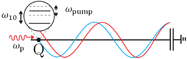
where characterizes the qubit location in a semi-infinite transmission line [corresponding to the blue curve in Fig. 1], and is proportional to the probe signal amplitude. Moreover, we should mention that if the qubit is “hidden” or “decoupled” from the transmission line, with .
To describe the qubit dynamics, we utilize the Lindblad equation, which in the charge basis with the Hamiltonian (4) has the form:
| (9) |
where is the density matrix, such that . The Lindblad superoperator describes the system relaxation induced by interactions with the environment,
| (10) |
where is the anticommutator. For a qubit there exist two relaxation channels: dephasing (described by ) and energy relaxation (described by ). In the energy basis the corresponding operators can be expressed in the following form:
| (11) |
with , , being the qubit relaxation, is the decoherence rate, is the pure dephasing rate.
III Energy and charge basis
In this section we will discuss the question related to the selection of an appropriate basis. As it was mentioned, the Hamiltonian (4) and the Lindnlad equation (9) were written in a charge basis, while the relaxations and are determined in the energy basis. So one should transfer Lindblad operators from the energy basis to the charge one. To study this question let’s rewrite the Hamiltonian (4) in the form:
| (12) |
where the constant component is equal to
| (13) |
and time-dependent part can be written as
| (14) |
In other words the Hamiltonian (4) can be considered as an effective Hamiltonian of a two-level system with tunneling amplitude , and excitation .
The transfer matrix which provides transfer from a charge basis to an energy one has a form:
| (16) |
where
| (17) |
The matrix diagonalizes time-independent part of the Hamiltonian (13):
| (18) |
where , — are eigenvalues of the Hamiltonian .
Therefore, one can transfer Lindblad superoperators from energy basis to the charge one by using the relation:
| (19) |
Substitution of Eqs. (11, 19) to the Lindblad equation (9) will give the necessary dependence , which is used for building theoretical plots.
IV Qubit interferometry
By solving Eq. (9), we get as a function of time , the pump frequency , the pump amplitude , the probe frequency , the signal amplitude . The occupation probability of the upper charge level is a function of all these parameters, . We can also calculate the dependencies for in the stationary regime by averaging the results over time.
To obtain the time-averaged values, we analyzed the curve to select the minimum time after which the amplitude of oscillations does not change. And then averaging was applied for the interval , where corresponds to the pulse off time. We determined that for our case and (see Ref. [Liul et al., 2023b] for more details).
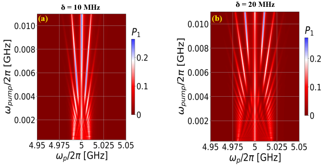
In this section, we theoretically investigate the dependence of the qubit upper charge level occupation probability on the pump frequency and the probe frequency . Note that the experimental study of such dependence was not conducted. But since one found the values of the fitting parameters in Ref. [Liul et al., 2023b] we can construct such a dependence. It is shown in Fig. 2, (a) corresponds to the pump amplitude , for (b) the pump amplitude is equal to . From the analysis of interferograms, it becomes clear that the larger the pumping amplitude , the larger the amplitude along the axis. Similar dependencies can be observed in Ref. [Wen et al., 2020], where only the stationary case was considered.
Such interferograms are useful not only for obtaining fitting parameters between theory and experiment, but they also play a key role in system characterization. In particular, they can help to:
-
•
estimate the system decoherence time;
-
•
provide a tool for calibrating signal strength during experimental studies;
-
•
open up new possibilities for multiphoton spectroscopy.
V Qubit dynamics
V.1 Dependence of the upper charge level occupation probability on the probe frequency for the case of Lindblad operators in the energy basis
This section presents the results of calculations for the case of Lindblad operators in the energy basis. Note, that this approach is not correct and the obtained theoretical dependencies are not consistent with the experimental ones, however, from a methodological point of view, it is useful to give such an example. Figure 3 shows the pictures obtained as a result of such calculations. This dependence corresponds to Fig. 4(d-f) in Ref. [Liul et al., 2023b].
From the comparison of the theoretical (Fig. 3(a-c)) and the corresponding experimental (Fig. 4(a-c) in Ref. [Liul et al., 2023b]) pictures, we can conclude that the Lindblad operators have to be transferred to the charge basis. The obtained dependencies have a behavior similar to the experimental ones, for example, resonances occur at both in the theory and in the experiment. However, unlike the experimental ones in the theoretical pictures, the resonance is slightly shifted from the line and it is more blurred (wider).
V.2 Dependence of the upper charge level occupation probability on the probe frequency and time
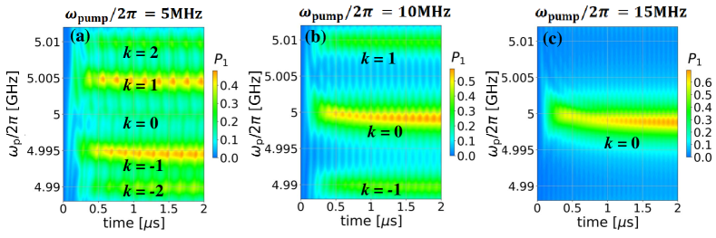
In the presented section, we will construct dependencies similar to those shown in the work [Liul et al., 2023b] in Fig. 4(d,e,f), but at lower values of the frequency of the pump signal . Figure 4 shows the obtained interferograms. The qubit is irradiated by pump signal with a frequency of (a) , (b) , (c) .
In Fig. 4(a), for the case , the resonance peaks are not distinguished, this may occur due to the fact that they are located too close to each other and therefore merge. For the Fig. 4(b), strong peaks are observed only at a distance from the line , for the Fig. 4(c) strong peaks are observed only at a distance from the line , while peaks at a distance of are weakly highlighted.
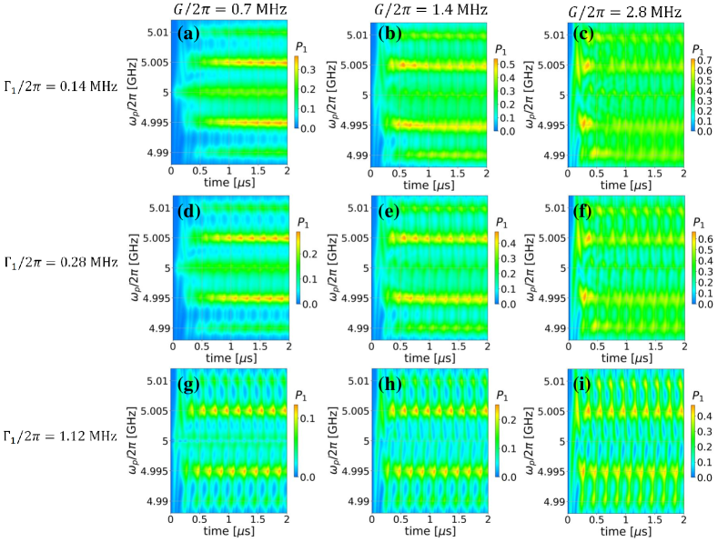
V.3 Dependence of the upper charge level occupation probability on the probe amplitude and the probe frequency for at different values of the probe amplitude and the relaxation rate
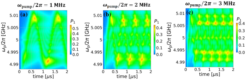
In the presented section, we will investigate the dependence of the upper charge level occupation probability on time and the probe frequency at different values of the probe amplitude and the relaxation rate for the pump frequency . For calculations, the pump amplitude is taken equal to . The resulting dependencies are shown in Fig. 5.
Analyzing the obtained dependencies, it can be concluded that with an increase of the relaxation rate at a fixed value of the probe amplitude (within a certain column we move from top to bottom), the resonances become less blurred, that is, their amplitude along the time axis decreases. This fact is understandable, because with an increase in the relaxation rate, the system quickly relaxes to the unexcited state, what is observed on the obtained dependencies.
For the case , the first resonances observed at 0.25 are clearly expressed, while for probe amplitude , the maximum value of the upper charge level occupation probability corresponds to the second and third resonances, while the first resonance is weakly highlighted. For and , during the first 1 the value of the upper charge level occupation probability has smaller values than for longer time values. In the case of and the first two resonances ( 0.5 ) are highlighted more weakly than the following ones.
VI Conclusions
We considered the dynamics and stationary mode of a transmon-type capacitive shunted qubit in front of a mirror, which is affected by two signals: probing and pumping.
To analyze the steady state, the upper charge level occupation probability was calculated as a function of the pump frequency and the probe frequency at the fixed pump amplitude and the probe amplitude . The resulting dependencies can be used to obtain fitting parameters; system decoherence time estimation; power calibration; studying multiphoton spectroscopy.
To analyze the dynamics, we plotted the dependencies of the upper charge level occupation probability on (a) time and the probe frequency at different pump frequencies ; (b) time and the probe frequency at different values of the probe amplitude and the relaxation rate for the pump frequency . The obtained results can be used in setting up future experiments.
The Lindblad equation with Lindblad superoperators in different bases: a charge and an energy one was solved. One concluded that the superoperators had to be in the charge basis, since the equation is also written in this basis. Such a comparison should be useful from the methodological point of view.
Acknowledgements.
The author acknowledge fruitful discussions with S. N. Shevchenko, A. I. Ryzhov, O. V. Ivakhnenko. The author was partially supported by the grant from the National Academy of Sciences of Ukraine for research works of young scientists (1/H-2023, 0123U103073).References
- Nielsen and Chuang (2010) M. A. Nielsen and I. L. Chuang, Quantum Computation and Quantum Information: 10th Anniversary Edition (Cambridge University Press, 2010).
- Kockum and Nori (2019) A. F. Kockum and F. Nori, “Quantum Bits with Josephson Junctions,” in Fundamentals and Frontiers of the Josephson Effect (Springer International Publishing, 2019) pp. 703–741.
- Oliver and Welander (2013) W. D. Oliver and P. B. Welander, “Materials in superconducting quantum bits,” MRS Bulletin 38, 816 (2013).
- Hoi et al. (2015) I.-C. Hoi, A. F. Kockum, L. Tornberg, A. Pourkabirian, G. Johansson, P. Delsing, and C. M. Wilson, “Probing the quantum vacuum with an artificial atom in front of a mirror,” Nat. Phys. 11, 1045–1049 (2015).
- Kannan et al. (2020) B. Kannan, M. J. Ruckriegel, D. L. Campbell, A. F. Kockum, J. Braumuller, D. K. Kim, M. Kjaergaard, P. Krantz, A. Melville, B. M. Niedzielski, A. Vepsalainen, R. Winik, J. L. Yoder, F. Nori, T. P. Orlando, S. Gustavsson, and W. D. Oliver, “Waveguide quantum electrodynamics with superconducting artificial giant atoms,” Nature 583, 775–779 (2020).
- Wen et al. (2018) P. Y. Wen, A. F. Kockum, H. Ian, J. C. Chen, F. Nori, and I.-C. Hoi, “Reflective amplification without population inversion from a strongly driven superconducting qubit,” Phys. Rev. Lett. 120, 063603 (2018).
- Xu et al. (2007) X. Xu, B. Sun, P. R. Berman, D. G. Steel, A. S. Bracker, D. Gammon, and L. J. Sham, “Coherent optical spectroscopy of a strongly driven quantum dot,” Science 317, 929–932 (2007).
- Wu et al. (1977) F. Y. Wu, S. Ezekiel, M. Ducloy, and B. R. Mollow, “Observation of amplification in a strongly driven two-level atomic system at optical frequencies,” Phys. Rev. Lett. 38, 1077–1080 (1977).
- Mirhosseini et al. (2019) M. Mirhosseini, E. Kim, X. Zhang, A. Sipahigil, P. B. Dieterle, A. J. Keller, A. Asenjo-Garcia, D. E. Chang, and O. Painter, “Cavity quantum electrodynamics with atom-like mirrors,” Nature 569, 692 (2019).
- Wen et al. (2019) P. Y. Wen, K.-T. Lin, A. F. Kockum, B. Suri, H. Ian, J. C. Chen, S. Y. Mao, C. C. Chiu, P. Delsing, F. Nori, G.-D. Lin, and I.-C. Hoi, “Large collective Lamb shift of two distant superconducting artificial atoms,” Phys. Rev. Lett. 123, 233602 (2019).
- Wilson et al. (2011) C. M. Wilson, G. Johansson, A. Pourkabirian, M. Simoen, J. R. Johansson, T. Duty, F. Nori, and P. Delsing, “Observation of the dynamical Casimir effect in a superconducting circuit,” Nature 479, 376–379 (2011).
- Hoi et al. (2013) I.-C. Hoi, A. F. Kockum, T. Palomaki, T. M. Stace, B. Fan, L. Tornberg, S. R. Sathyamoorthy, G. Johansson, P. Delsing, and C. M. Wilson, “Giant Cross-Kerr effect for propagating microwaves induced by an artificial atom,” Phys. Rev. Lett. 111, 053601 (2013).
- Hoi et al. (2012) I.-C. Hoi, T. Palomaki, J. Lindkvist, G. Johansson, P. Delsing, and C. M. Wilson, “Generation of nonclassical microwave states using an artificial atom in 1D open space,” Phys. Rev. Lett. 108, 263601 (2012).
- Karpov et al. (2020) D. Karpov, V. Monarkha, D. Szombati, A. Frieiro, A. Omelyanchouk, E. Il’ichev, A. Fedorov, and S. Shevchenko, “Probabilistic motional averaging,” Eur. Phys. J. B 93, 49 (2020).
- Hoi et al. (2011) I.-C. Hoi, C. M. Wilson, G. Johansson, T. Palomaki, B. Peropadre, and P. Delsing, “Demonstration of a single-photon router in the microwave regime,” Phys. Rev. Lett. 107, 073601 (2011).
- Ivakhnenko et al. (2023) O. V. Ivakhnenko, S. N. Shevchenko, and F. Nori, “Nonadiabatic Landau-Zener-Stückelberg-Majorana transitions, dynamics and interference,” Phys. Rep. 995, 1–89 (2023).
- Shevchenko (2019) S. N. Shevchenko, Mesoscopic Physics meets Quantum Engineering (World Scientific, Singapore, 2019).
- Liul et al. (2023a) M. P. Liul, A. I. Ryzhov, and S. N. Shevchenko, “Rate-equation approach for a charge qudit,” Eur. Phys. J.: Spec. Top. (2023a).
- Campbell et al. (2020) D. L. Campbell, Y.-P. Shim, B. Kannan, R. Winik, D. K. Kim, A. Melville, B. M. Niedzielski, J. L. Yoder, C. Tahan, S. Gustavsson, and W. D. Oliver, “Universal nonadiabatic control of small-gap superconducting qubits,” Phys. Rev. X 10, 041051 (2020).
- Liul et al. (2023b) M. P. Liul, C.-H. Chien, C.-Y. Chen, P. Y. Wen, J. C. Chen, Y.-H. Lin, S. N. Shevchenko, F. Nori, and I.-C. Hoi, “Coherent dynamics of a photon-dressed qubit,” Phys. Rev. B 107, 195441 (2023b).
- Wen et al. (2020) P. Y. Wen, O. V. Ivakhnenko, M. A. Nakonechnyi, B. Suri, J.-J. Lin, W.-J. Lin, J. C. Chen, S. N. Shevchenko, F. Nori, and I.-C. Hoi, “Landau-Zener-Stückelberg-Majorana interferometry of a superconducting qubit in front of a mirror,” Phys. Rev. B 102, 075448 (2020).
- Silveri et al. (2015) M. Silveri, K. Kumar, J. Tuorila, J. Li, A. Vepsalainen, E. Thuneberg, and G. Paraoanu, “Stueckelberg interference in a superconducting qubit under periodic latching modulation,” New J. Phys. 17, 043058 (2015).