Interpolation for Robust Learning:
Data Augmentation on Wasserstein Geodesics

Abstract

We propose to study and promote the robustness of a model as per its performance through the interpolation of training data distributions. Specifically, (1) we augment the data by finding the worst-case Wasserstein barycenter on the geodesic connecting subpopulation distributions of different categories. (2) We regularize the model for smoother performance on the continuous geodesic path connecting subpopulation distributions. (3) Additionally, we provide a theoretical guarantee of robustness improvement and investigate how the geodesic location and the sample size contribute, respectively. Experimental validations of the proposed strategy on four datasets, including CIFAR-100 and ImageNet, establish the efficacy of our method, e.g., our method improves the baselines’ certifiable robustness on CIFAR10 up to $7.7\%$ , with $16.8\%$ on empirical robustness on CIFAR-100. Our work provides a new perspective of model robustness through the lens of Wasserstein geodesic-based interpolation with a practical off-the-shelf strategy that can be combined with existing robust training methods.

Jiacheng Zhu¹

Jielin Qiu¹

Aritra Guha²

Zhuolin Yang³

XuanLong Nguyen⁴

Bo Li³

Ding Zhao¹

Carnegie Mellon University¹, AT&T Chief Data Office²

University of Illinois at Urbana-Champaign³, University of Michigan⁴

\doparttoc\faketableofcontents

1 Introduction

Deep neural networks (DNNs) have shown tremendous success in an increasing range of domains such as natural language processing, image classification & generation and even scientific discovery (e.g. (Bahdanau et al., 2014; Krizhevsky et al., 2017; Ramesh et al., 2022)). However, despite their super-human accuracy on training datasets, neural networks may not be robust. For example, adding imperceptible perturbations, e.g., adversarial attacks, to the inputs may cause neural networks to make catastrophic mistakes (Szegedy et al., 2014; Goodfellow et al., 2014). Conventional defense techniques focus on obtaining adversarial perturbations (Carlini & Wagner, 2017; Goodfellow et al., 2014) and augmenting them to the training process. For instance, the projected gradient descent (PGD) (Madry et al., 2018), which seeks the worst-case perturbation via iterative updates, marks a category of effective defense methods.

Recent works show that additional training data, including data augmentation and unlabeled datasets, can effectively improve the robustness of deep learning models (Volpi et al., 2018; Rebuffi et al., 2021). Despite augmenting worst-case samples with gradient information, an unlabeled, even out-of-distribution dataset may also be helpful in this regard (Carmon et al., 2019; Bhagoji et al., 2019). Among available strategies, Mixup (Zhang et al., 2018), which interpolates training samples via convex combinations, is shown to improve both the robustness and generalization (Zhang et al., 2021). Moreover, Gaussian noise is appended to training samples to achieve certifiable robustness (Cohen et al., 2019), which guarantees the model performance under a certain degree of perturbation. However, most aforementioned approaches operate on individual data samples (or pairs) and require the specification of a family of augmentation policies, model architecture, and additional datasets. Thus, the robustness can hardly be generalizable, e.g., to out-of-sample data examples. To this end, we are curious: Can we let the underlying data distribution guide us to robustness?

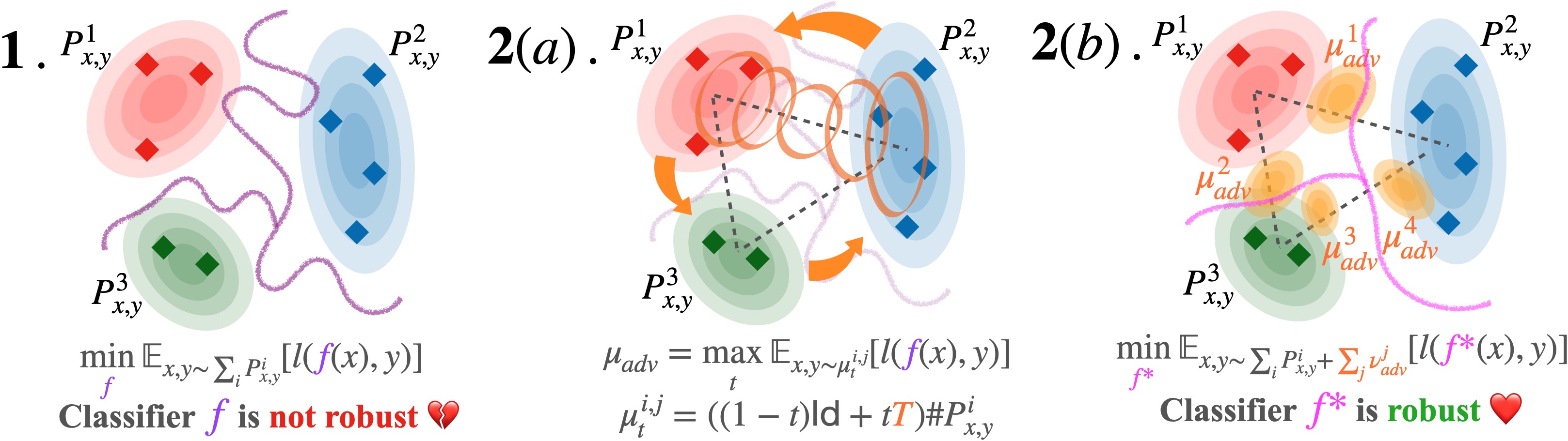
We propose a framework to augment synthetic data samples by interpolating the underlying distributions of the training datasets. Specifically, we find the worst-case interpolation distributions that lie on the decision boundary and improve the model’s smoothness with samples from these distributions. This is justified by the fact that better decision margin (Kim et al., 2021a) and boundary thickness (Moosavi-Dezfooli et al., 2019) are shown to benefit robustness.

The probabilistic perspective allows us to formulate the distribution interpolation as barycenter distribution on Wasserstein geodesics, where the latter can be reviewed as a dynamic formulation of optimal transport (OT) (Villani, 2009). This formulation has the following benefits: (a). It nicely connects our worst-case barycenter distribution to distributionally robust optimization (Duchi & Namkoong, 2021) on the geodesic and substantiates our method’s benefit in promoting robustness. (b). The geodesic provides a new protocol to assess one model’s robustness beyond the local area surrounding individual data points. (c). Our data augmentation strategy also exploits the local distribution structure by generalizing the interpolation from (mostly Euclidean) feature space to probability space. (d). Apart from most OT use cases that rely on coupling, we reformulate the objective to include explicit optimal transport maps following McCann’s interpolation (McCann, 1997). This enables us to deal with out-of-sample data and appreciate the recent advances in OT map estimation (Perrot et al., 2016; Zhu et al., 2021; Amos, 2022), neural OT map estimators (Makkuva et al., 2020; Seguy et al., 2017; Fan et al., 2021) for large-scale high-dimensional datasets, and OT between labeled datasets (Alvarez-Melis & Fusi, 2020; Fan & Alvarez-Melis, 2022).

1.1 Related Work

Interpolation of data distributions

Gao & Chaudhari (2021) propose a transfer distance based on the interpolation of tasks to guide transfer learning. Meta-learning with task interpolation (Yao et al., 2021), which mixes features and labels according to tasks, also effectively improves generalization. For gradual domain adaptation, Wang et al. (2022) interpolate the source dataset towards the target in a probabilistic fashion following the OT schema. Moreover, the interpolation of environment distribution Huang et al. (2022) is also effective in reinforcement learning. The recently proposed rectified flow (Liu et al., 2022) facilities a generating process by interpolating data distributions in their optimal paths. In addition, the distribution interpolant (Albergo & Vanden-Eijnden, 2022) has motivated an efficient flow model which avoids the costly ODE solver but minimizes a quadratic objective that controls the Wasserstein distance between the source and the target. Recently, the interpolation among multiple datasets realized on generalized geodesics (Fan & Alvarez-Melis, 2022) is also shown to enhance generalizability for pretraining tasks. Most aforementioned works focus on the benefit of distribution interpolation in generalization.

On the other hand, Mixup (Zhang et al., 2018), which augments data by linear interpolating between two samples, is a simple yet effective data augmentation method. As detailed in survey (Cao et al., 2022; Lewy & Mańdziuk, 2022), there are plenty of extensions such as CutMix (Yun et al., 2019), saliency guided (Uddin et al., 2020), AugMix (Hendrycks et al., 2019), manifold mixup (Verma et al., 2019), and so on (Yao et al., 2022). A few studies have explored the usage of optimal transport (OT) ideas within mixup when interpolating features (Kim et al., 2020; 2021b). However, those methods focus on individual pairs, thus neglecting the local distribution structure of the data. One recent work (Greenewald et al., 2021) also explores mixing multiple-batch samples with OT alignment. Although their proposed K-mixup better preserves the data manifold, our approach aims to determine the worst-case Wasserstein barycenter, achieved through an interpolation realized by transport maps.

Data augmentation for robustness.

Augmentation of data(Rebuffi et al., 2021; Volpi et al., 2018) or more training data (Carmon et al., 2019; Sehwag et al., 2021) can improve the performance and robustness of deep learning models. However, (Schmidt et al., 2018) show that sample complexity for robust learning may be prohibitively large when compared to standard learning. Moreover, with similar theoretical frameworks, recent papers (Deng et al., 2021; Xing et al., 2022) further establish theoretical justifications to characterize the benefit of additional samples for model robustness. However, additional data may not be available; in this work, we therefore use a data-dependent approach to generate additional data samples.

1.2 Contributions

Our key contributions are as follows. We propose a data augmentation strategy that improves the robustness of the label prediction task by finding worst-case data distributions on the interpolation within training distributions. This is realized through the notion of Wasserstein geodesics and optimal transport map, and further strengthened by connection to DRO and regularization effect. Additionally, we also provide a theoretical guarantee of robustness improvement and investigate how the geodesic location and the sample size contribute, respectively. Experimental validations of the proposed strategy on four datasets including CIFAR-100 and ImageNet establish the efficacy of our method.

2 Preliminaries

Consider a classification problem on the data set $S=\{(x_{1},y_{1}),...,(x_{n},y_{n})\}$ , where $x_{i}\in\mathcal{X}\subseteq\mathbb{R}^{d}$ and $y_{i}\in\mathcal{Y}\subseteq\mathbb{R}^{y}$ are drawn i.i.d from a joint distribution $\mathcal{P}^{all}_{x,y}$ . Having a loss criteria $l(\cdot,\cdot):\mathcal{Y}\times\mathcal{Y}\mapsto\mathbb{R}$ , the task is to seek a prediction function $f_{\theta}:\mathbb{R}^{d}\mapsto\mathbb{R}^{y}$ that minimizes the standard loss $L(\theta)=\mathbb{E}_{x,y\sim\mathcal{P}^{all}_{x,y}}[l(f_{\theta}(x),y)]$ , and in practice people optimize the empirical loss $\hat{L}(\theta)=1/n\sum_{i=1}^{n}l(f(x_{i}),y_{i})$ following the Empirical Risk Minimization (ERM). In large-scale classification tasks such as $k$ -class image classification, the label is the one-hot encoding of the class as $y_{i}\in\{0,1\}^{k}:=\mathbb{R}^{k}$ and $l$ are typically cross-entropy loss.

Adversarial training & distributional robustness

Typically, adversarial training is a minimax optimization problem (Madry et al., 2018) which finds adversarial examples $x+\delta$ within a perturbation set $\mathcal{S}=\{\delta:\|\delta\|_{\infty}\leq\epsilon,\epsilon>0\}$ . While finding specific attack examples is effective, there are potential issues such as overfitting on the attack pattern (Kurakin et al., 2016; Xiao et al., 2019; Zhang & Wang, 2019).

An alternative approach is to capture the distribution of adversarial perturbations for more generalizable adversarial training (Dong et al., 2020). In particular, the optimization problem solves a distributional robust optimization (Duchi & Namkoong, 2021; Weber et al., 2022) as follows:

\min_{\theta}\sup_{Q_{x,y}\in\mathcal{U}_{P}}\mathbb{E}_{x,y\sim Q_{x,y}}[l(f_{\theta}(x),y)],

(1)

where $\mathcal{U}_{P}\subseteq\mathcal{P(Z)}$ is a set of distributions with constrained support. Intuitively, it finds the worst-case optimal predictor $f^{*}_{\theta}$ when the data distribution $P$ is perturbed towards an adversarial distribution $\mathcal{U}_{P}$ . However, the adversarial distribution family needs to be properly specified. In addition, adversarial training may still have unsmooth decision boundaries (Moosavi-Dezfooli et al., 2019), thus, are vulnerable around unobserved samples.

Optimal transport

Given two probability distributions $\mu,\nu\in\mathcal{M}(\mathcal{X})$ , where $\mathcal{M}(\mathcal{X})$ is the set of Borel measures on $\mathcal{X}$ . The optimal transport (OT) (Villani, 2009) finds the optimal joint distribution and quantifies the movement between $\mu$ and $\nu$ . Particularly, the Wasserstein distance is formulated as $W_{p}(\mu,\nu):=(\inf_{\pi\in\Pi}\int_{\mathcal{X}\times\mathcal{X}}d^{p}(x,y)d\pi(x,y))^{1/p},$ where $d(\cdot,\cdot):\mathcal{X}\times\mathcal{X}\mapsto\mathbb{R}^{+}$ is the ground metric cost function, and $\Pi$ denotes set of all joint probability measures on $\mathcal{X}\times\mathcal{X}$ that have the corresponding marginals $\mu$ and $\nu$ .

Wasserstein barycenter and geodesic

Equipped with the Wasserstein distance, we can average and interpolate distributions beyond the Euclidean space. The Wasserstein barycenter $\mu^{\{\nu_{i}\}}_{\alpha}$ of a set of measures $\{\nu_{1},...,\nu_{N}\}$ in a probability space $\mathbb{P}\subset\mathcal{M}(\mathcal{X})$ is a minimizer of objective $U^{N}_{wb}$ over $\mathbb{P}$ , where

\displaystyle\small U^{N}_{wb}(\mu):=\sum_{i=1}^{N}\alpha_{i}W(\mu,\nu_{i}),

(2)

and $\alpha_{i}$ are the weights such that $\sum\alpha_{i}=1$ and $\alpha_{i}>0$ . Let $\nu_{0}$ and $\nu_{1}$ be two measure with an existing optimal transportation map, $T$ , satisfying $\nu_{1}=T\#\nu_{0}$ and $W^{2}_{2}(\nu_{0},\nu_{1})=\int_{\mathcal{X}}\|x-T(x)\|^{2}d\nu_{0}$ . Then, for each $t$ , the barycenter distribution(denoted by $\mu_{t}$ ) corresponding to $\alpha_{0}=t,\alpha_{1}=1-t$ in Eq.(2), lies on the geodesic curve connecting $\nu_{0}$ and $\nu_{1}$ . Moreover, (McCann, 1997),

\displaystyle\small\mu_{t}:=((1-t)\text{Id}+tT)\#\nu_{0},

(3)

where Id is the identity map. While the above McCann’s interpolation is defined only for two distributions, the Wasserstein barycenter eq. (2) can be viewed as a generalization to $N\geq 2$ marginals. To this point, we are able to look for adversarial distributions leveraging such interpolation.

Refer to caption — Figure 1: 1: For a classification problem, the data samples give empirical access to the underlying data distribution, which is a mixture of distinct subpopulation distributions. 2(a): The inner maximization step finds the worst-case Wasserstein barycenter on the geodesic. 2(b): The outer minimization step updates the predictive function with augmented samples.

3 Adversarial robustness by interpolation

For a $k$ -classification task, it is natural to view the data of each category are samples from distinct distributions $P^{all}_{x,y}=\sum^{k}_{i}P^{i}_{x,y}$ . Following eq.(1), we can write the following minimax objective

\displaystyle\min_{f}\max_{\alpha}\mathbb{E}_{x,y\sim U^{wb}(\alpha)}\left[l(f(x),y)\right]

(4)

where $U^{wb}(\alpha)$ is the Wasserstein barycenter (eq. 2), in other words, the interpolation of different category distributions. In fact, this corresponds to a special case of DRO eq.(1) as shown in the below proposition, and naturally corresponds to the adversarial distribution within a particular Wasserstein ball, for distributional robustness.

Proposition 3.1.

Suppose the original data $\{{X}_{i},{Y}_{i},\}_{i=1}^{{n_{0}}}$ are iid with distribution satisfying $X|Y=y\sim\nu_{\mu}(X|Y)=N_{d}(y\mu,\sigma^{2}I)$ , $Y\sim\nu(Y)=U\{-1,1\}$ . Assume the loss function is given by $l(f(x),y)=\mathbbm{1}(f(x)\neq y)$ . We consider $f(x)=f_{\alpha,\beta}(x)$ of the form $\text{sign}(\alpha^{\prime}x+\beta)$ .Then the following holds

	$\displaystyle\max_{A(\nu_{\mu},\epsilon)}\inf_{\alpha,\beta}\mathbb{E}_{(X,Y)\sim\eta(X\|Y)\nu(Y)}l(f_{(\alpha,\beta)}(X),Y)$	(5)
$\displaystyle=$	$\displaystyle inf_{\alpha,\beta}\max_{A(\nu_{\mu},\epsilon)}\mathbb{E}_{(X,Y)\sim\eta(X\|Y)\nu(Y)}l(f_{(\alpha,\beta)}(X),Y)$
$\displaystyle=$	$\displaystyle\mathbb{E}_{(X,Y)\sim\nu_{(1-\epsilon)\mu}(X\|Y)\nu(Y)}l(f_{(\mu,0)}(X),Y).$

Here, $A(\nu_{\mu},\epsilon)=\{\eta(X|Y):\eta(\cdot|Y)$ is Gaussian, $W(\eta(X|Y),\nu_{\mu}(X|Y))\leq\epsilon,\ \forall Y\in\{-1,1\}\}$ .

This proposition, whose proof is discussed in Section A.4.

3.1 Data augmentation: worst-case interpolation

In this section, we proceed to device computation strategies for the worst-case barycenter approach. Akin to robust training methods that seek adversarial examples approximately, such as PGD (Madry et al., 2018) and FGSM (Goodfellow et al., 2014), our paradigm learns an adversarial distribution (Dong et al., 2020) and then samples from these distributions.

Here we make an important choice by focusing on the interpolation between $K=2$ distributions rather than a generalized $K$ -margin barycenter. To date, efficient computational solutions for for multimarginal OT (MOT) are still nascent (Lin et al., 2022). Solving an MOT with linear programming would scale to $O(n^{K})$ , and would be more costly when we want to solve for (free-support) barycenters to facilitate robustness in deep learning pipelines. Focusing on $K=2$ not only (1) allows us to focus on the decision boundary between the different categories of data, and even to deepen our understanding with theoretical analysis for robustness. (2) Achieve computation efficiency by leveraging established OT algorithms when iterating between pairs of distributions, as illustrated in Fig.(1).

Thus, our data augmentation strategy is to sample data from the worst-case adversarial Wasserstein barycenter $\{\hat{x}_{i},\hat{y}_{i}\}\sim\mu^{\{P_{0},P_{1}\}}_{adv}$ , which can be obtained as an inner maximization problem,

\displaystyle\mu^{\{P_{0},P_{1}\}}_{adv}

\displaystyle:=\max_{t\in[0,1]}\mathbb{E}_{x,y\sim\mu^{\{P_{0},P_{1}\}}_{t}}\left[l(f_{\theta}(x),y)\right].

(6)

Despite a list of recent advances (Villani, 2009; Korotin et al., 2022a; Fan et al., 2020), the usage of Wasserstein barycenter may still be limited by scalability, and those solvers are more limited since we are optimizing the location of barycenters. However, thanks to the celebrated properties (Brenier, 1991; McCann, 1997), which connects the Monge pushforward map with the coupling, we can avoid the intractable optimization over $\mu_{t}$ and turn to the training distribution with a transport map.

Interpolation with OT map

When $\nu_{0},\nu_{1}\in\mathcal{M}(\mathcal{X})$ , $\nu_{1}$ is absolutely continuous with respect to $\nu_{0}$ . Let $\mu(t)=\{\mu_{t}\}_{0\leq t\leq 1}$ be the geodesic of displacement interpolation, then we have a unique and deterministic interpolation $\mu_{t}=(T_{t})\#P^{0}$ , where $T_{t}(x):=(1-t)x+tT(x)$ and convex function $T(\cdot)$ is the optimal transport map (Villani, 2009). Thus, the following proposition yields an objective for finding the worst-case barycenter:

Proposition 3.2.

Consider a factored map $T^{xy}:=(T^{x},T^{y}):\mathbb{R}^{d}\times\mathbb{R}^{y}\mapsto\mathbb{R}^{d}\times\mathbb{R}^{y}$ defined as $T(\cdot,*):=(T^{x}(\cdot),T^{y}(*))$ . Consequently, rewriting Eq, (6) with this above map yields

$\displaystyle\tilde{\mu}^{\{P_{0},P_{1}\}}_{adv}:=$	$\displaystyle\max_{t\in[0,1]}\mathbb{E}_{x,y\sim P^{0}}\left[l(f_{\theta}(T^{x}_{t}(x)),T^{y}_{t}(y))\right]$	(7)
where,	$\displaystyle T^{x}_{t}(x)=(1-t)x+tT^{x}(x),$
	$\displaystyle T^{y}_{t}(y)=(1-t)y+tT^{y}(y)$

such that the map $T^{xy}$ satisfies the Monge problem $\min_{T^{xy}\#P^{0}=P^{1}}\mathbb{E}_{x,y\sim P^{0}}[\mathcal{D}(\{x,y\},T^{xy}(\{x,y\}))^{2}]$ . Here $\mathcal{D}(\{x_{1},y_{1}\},\{x_{2},y_{2}\})=d(x_{1}-y_{1})+{L}(y_{1},y_{2})$ is a measure that combines the distance between samples the discrepancy between $y_{1}$ and $y_{2}$ Courty et al. (2017b). We note here this joint cost is separable and the analysis of the generic joint cost function is left for future studies (Fan et al., 2021; Korotin et al., 2022b).

The benefits of this formulation: (1) Rather than the barycenter, the problem uses the OT map estimation where a lot of previous works have concerned efficiency (Perrot et al., 2016), scalability (Seguy et al., 2017) and convergence (Manole et al., 2021). (2) The transport map can be estimated solely on data and stored regardless of the supervised learning task. Moreover, the map can project out-of-sample points, which improves the generalization. (3) For the case where real data lies on a complex manifold, it is necessary to utilize an embedding space. Specifically, we perform the computation of Wasserstein geodesic and interpolation in an embedding space that is usually more regularized (Kingma & Welling, 2013). (4) Such OT results on labeled data distributions have been shown effective (Alvarez-Melis & Fusi, 2020; 2021; Fan & Alvarez-Melis, 2022) in transfer learning tasks while we first investigate its distributional robustness. Also, interestingly, when ignoring the expectation and defining the map as $T^{x}(x^{0}):=x^{1}$ , $T^{y}(y^{0}):=y^{1}$ , such interpolation coincides with the popular mixup (Zhang et al., 2018) which is simple but effective even on complicated datasets.

3.2 Implicit regularization: geodesic smoothness

Data augmentation is, in general, viewed as implicit regularization (Rebuffi et al., 2021). However, our augmentation policy also motivates an explicit regularization term to enhance the training of deep neural networks.

For a given predictive function $f^{*}_{\theta}:\mathbb{R}^{d}\mapsto\mathbb{R}^{y}$ and a loss criterion $l(\cdot,\cdot):\mathcal{Y}\times\mathcal{Y}\mapsto\mathbb{R}$ , now we consider the following performance geodesic,

\small\text{R}^{\text{g}}_{f^{*}_{\theta},l}(t):=\mathbb{E}_{x,y\sim\mu(t)}\left[l(f(x),y)\right],

(8)

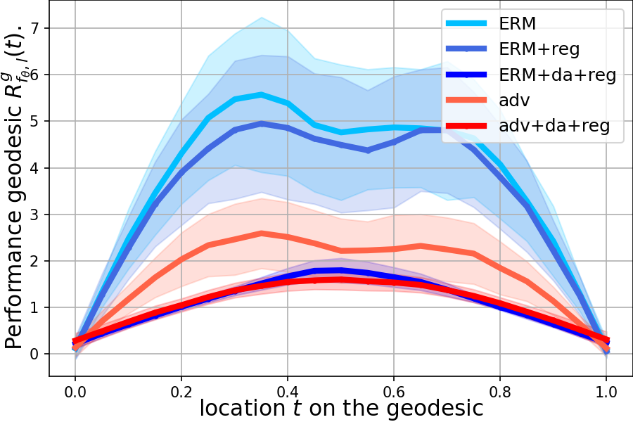
which quantifies the loss associated with the prediction task, where $\mu(t)$ is the displacement interpolation as stated after Eq. (6). The geodesic loss $\text{R}^{\text{geo}}_{f^{*}_{\theta}}$ provides us a new lens through which we can measure, interpret, and improve a predictive model’s robustness from a geometric perspective.

Since the geodesic is a smooth and continuous path connecting $P^{0},P^{1}$ , The factorized geodesic interpolation $T^{xy}$ Eq. (6) allows us to formulate a new metric $\text{Reg}^{T^{xy}}_{l}$ that measures the change of a classifier $f^{*}_{\theta}$ , under criteria $l(\cdot,\cdot)$ when gradually transporting from $P^{0}$ to $P^{1}$ .

\displaystyle\int_{0}^{1}\left|\frac{d}{dt}\int_{\mathcal{X}\times\mathcal{Y}}l(f_{\theta}(T^{x}_{t}(x),T^{y}_{t}(y))dP^{0}(x,y)\right|dt=\int_{0}^{1}\left|\frac{d}{dt}\text{R}^{T^{xy}}_{f_{\theta},l}(t)\right|dt

(9)

where $\text{R}^{T}_{f_{\theta},l}(t)=\mathbb{E}_{x,y\sim P^{0}}\left[l(f^{*}_{\theta}(T^{x}_{t}(x)),T^{y}_{t}(y))\right]$ is the expected loss of $f^{*}_{\theta}$ at the location $t$ on the geodesic interpolation. Thus, to robustify a classifier $f_{\theta}$ , we propose to use the following regularization, which promotes the smoothness derivative along the geodesic.

\displaystyle\text{Reg}^{T}_{l}(f_{\theta}):=\int_{0}^{1}\left|\frac{d}{dt}\text{R}^{T}_{f_{\theta},l}(t)\right|dt,\text{ (geodesic regularizer) }

(10)

Proposition 3.3 (Geodesic performance as data-adaptive regularization).

Consider the following minimization

\min_{f\in\mathcal{H}}\mathbb{E}_{x,y\sim P}[l(f(x),y)]+\frac{\lambda_{1}}{2}\text{Reg}^{\hat{T}}_{l}(f)^{2}+\frac{\lambda_{2}}{2}\|f\|^{2}_{\mathcal{H}}.

where $\mathcal{H}$ is space of function. When the data distribution is $P:=1/2P_{0}+1/2P_{1}$ and $P_{0}=\mathcal{N}(-\mu,I),P_{1}=\mathcal{N}(\mu,T)$ . The objective has the following form:

\min_{\theta}\mathcal{L}(\theta):=-\langle\theta,\mu\rangle+\frac{\lambda_{1}}{2}|\langle\theta,\mu\rangle|^{2}+\frac{\lambda_{2}}{2}\|\theta\|^{2}_{2}

The optimal solution $f$ corresponding to data assumption has the closed form $\theta^{*}=(\lambda_{1}\mu\otimes\mu+\lambda_{2}I_{m})^{-1}\mu,$ where $\otimes$ refers to the outer product.

The illustrative result above indicates our geodesic regularizer is a data-depend regularization adjusted by the underlying data distributions. This agrees with the recent theoretical understanding of mixup and robustness (Zhang et al., 2021). In addition, existing robustness criteria (empirical and certified robustness) focus on the local area of individual samples within a perturbation ball $\mathcal{S}=\{\delta:\|\delta\|_{\infty}\leq\epsilon,\epsilon>0\}$ without considering the robustness behavior of $f_{\theta}$ while transitioning from $P^{0}_{x,y}$ to $P^{1}_{x,y}$ . The interpolation provides a new perspective for robustness, as shown in Fig.(2).

3.3 Computation and implementation

OT map estimation

Our formulation allows us to leverage off-the-shelf OT map estimation approaches. Despite recent scalable and efficient solutions that solve the Monge problem (Seguy et al., 2017), withGAN (Arjovsky et al., 2017), ICNN (Makkuva et al., 2020), flow (Huang et al., 2020; Makkuva et al., 2020; Fan et al., 2021), and so on (Korotin et al., 2022b; Bunne et al., 2022). As the first step, in this work, we refer to barycentric projection (Ambrosio et al., 2005) thanks to its flexibility (Perrot et al., 2016) and recent convergence understandings (Manole et al., 2021; Pooladian & Niles-Weed, 2021). Specifically, we are not given access to the probability distributions $P^{0}$ and $P^{1}$ , but only samples $\{(x^{0}_{i},y^{0}_{i})\}_{i=1}^{n}\sim P^{0}_{xy}$ and $\{(x^{1}_{i},y^{1}_{i})\}_{i=1}^{n}\sim P^{1}_{xy}$ . When an optimal map $T_{0}\in\{T:\mathcal{X}\times\mathcal{Y}\mapsto\mathcal{X}\times\mathcal{Y}|T\#P^{0}=P^{1}\}$ exists, we want an estimator $\hat{T}_{n}$ with empirical distributions $\hat{P}^{0}_{xy,n}$ and $\hat{P}^{1}_{xy,n}$ . This problem is usually regarded as the two-sample estimation problem (Manole et al., 2021). Among them, the celebrated Sinkhorn algorithm (Cuturi, 2013) solves the entropic Kantorovich objective efficiently $\hat{\pi}{\epsilon,n}:=\arg\min_{\pi\in\Pi(\mathbb{R}^{n\times n})}\langle\pi,M\rangle+\epsilon H(\pi)$ , where $H(\pi):=-\sum_{ij}\pi_{ij}\log\pi_{ij}$ is the negative entropy, provides an efficient $O(n^{2})$ solution. Furthermore, It was shown in Section 6.2 of (Pooladian & Niles-Weed, 2021) that an entropy-regularised map (given by $\hat{T}_{\epsilon,{n}}$ ) for empirical distributions can approximate the population transportation map efficiently.

From the computation perspective, $T_{\epsilon,n}$ can be realized through the entropically optimal coupling (Cuturi, 2013) $\pi^{*}_{e}$ as $\hat{T}_{\epsilon,n}(X_{0})=\text{diag}(\pi^{*}\mathbf{1}_{n_{1}})^{-1}\pi^{*}_{\epsilon}X_{1}$ . Since we assume the samples are drawn i.i.d, then $\hat{T}_{\epsilon,n}(X_{0})=n_{0}\pi^{*}X_{1}$ . At this point, we can have the geodesic interpolation computed via regularized OT as

\displaystyle\hat{T}^{xy}_{t}:=\begin{cases}\hat{T}^{x}_{t}(X_{0})&=(1-t)X_{0}+t\hat{T}_{\epsilon,n}(X_{0}),\\ \hat{T}^{y}_{t}(Y_{0})&=(1-t)Y_{0}+tY_{1}\end{cases}

(11)

Since the labels $Y^{i}$ have a Dirac distribution within each $P_{i}$ , we utilize the map $T^{y}(y^{0}):=y^{1}$ . With such closed-form interpolation, we then generate samples by optimizing Eq. (7) using numerical methods such as grid search. Notice that, when setting $T^{x}(X_{0}):=X_{1}$ then the geodesic turns into the mixup however it can not deal with the case where we have different numbers of samples $n_{0}\neq n_{1}$ .

Regularization

With the aforementioned parameterization, we thus have the following expression for the smoothness regularizer $\text{Reg}^{T}_{l}(f_{\theta})$ .

		$\displaystyle\text{Reg}^{\hat{T}}_{l}(f_{\theta})=\int_{0}^{1}\left\|\frac{d}{dt}\text{R}^{T^{xy}}_{f_{\theta},l}(t)\right\|dt\text{ {} where {} }\frac{d}{dt}\text{R}^{T^{xy}}_{f_{\theta},l}(t)$		(12)
		$\displaystyle=\int\frac{dL}{d\tilde{y}}\nabla f_{\theta}((1-t)x+t\hat{T}_{\epsilon,n}(x))(\hat{T}_{\epsilon,n}(x)-x)dP^{0}(x,y)$		(12)

where $\tilde{y}=f_{\theta}((1-t)x+t\hat{T}(x))$ is the predicted target, $L=l(\tilde{y},\hat{T}^{y}_{t}(y))$ measures the loss with regard to the interpolated target. This regularizer can be easily computed with the Jacobian of $f_{\theta}$ on mixup samples. In fact, we regularize the inner product of the expected loss, the Jacobian on interpolating samples, and the difference of $\hat{T}_{\epsilon,n}(x_{0})-x_{0}$ . In fact, Jacobian regularizer has already been shown to improve adversarial robustness (Hoffman et al., 2019)

Manifold and feature space

The proposed data augmentation and regularization paradigms using the OT formulation have nice properties when data lie in a Euclidean space. However, the real data may lie on a complex manifold. In such a scenario, we can use an embedding network $\phi:\mathcal{X}\mapsto\mathcal{Z}$ that projects it to a low-dimensional Euclidean space $Z\in\mathbb{R}^{z}$ and a decoder network $\psi:\mathcal{Z}\mapsto\mathcal{X}$ . Similarly, data augmentation may be carried out via

\displaystyle\tilde{\mu}^{\{P_{0},P_{1}\}}_{adv}=

\displaystyle\max_{t\in[0,1]}\mathbb{E}_{x,y\sim P^{0}}\left[l(f_{\theta}(\psi(T^{x}_{t}(\phi(x)))),T^{y}_{t}(y))\right].

(13)

Also, regularize the geodesic on the manifold

		$\displaystyle\text{Reg}^{\hat{T}}_{l}(f_{\theta})=\int_{0}^{1}\left\|\frac{d}{dt}\text{R}^{T^{xy}}_{f_{\theta},l}(t)\right\|dt{\text{, {} where }}\frac{d}{dt}\text{R}^{T^{xy}}_{f_{\theta},l}(t)$		(14)
		$\displaystyle=\frac{1}{n}\frac{dL}{d\tilde{y}}\nabla f_{\theta}((1-t)\phi(X_{0})+tn\pi^{}_{\epsilon}\phi(X_{1}))(n\pi^{}_{\epsilon}\phi(X_{1})-\phi(X_{0})).$		(14)

In fact, such a method has shown effectiveness in Manifold Mixup (Verma et al., 2019) since a well-trained embedding helps create semantically meaningful samples than mixing pixels, even on a Euclidean distance that mimics Wasserstein distance (Courty et al., 2017a). Recent advances in representation learning (Radford et al., 2021) also facilitate this idea. In this work, we also adopt Variational Autoencoder (VAE) (Kingma & Welling, 2013) and pre-trained ResNets to obtain the embedding space. We follow a standard adversarial training scheme where we iteratively (a) update the predictor $f_{\theta}$ with objective $\min_{\theta}\mathbb{E}_{x_{i},y_{i}\sim\sum P^{i}+\sum\nu_{adv}[l(f_{\theta}(x),y)]}+\lambda\text{Reg}(f_{\theta})$ , where the geodesic regularization $\text{Reg}(f_{\theta})$ is computed via Eq.(LABEL:eq:comput_reg). (b) Find and store the augmented data by maximizing the equation (6). A pseudocode Algo.(2) is attached in the Appendix.

Scalability and batch OT

To handle large-scale datasets, we follow the concept of minibatch optimal transport (Fatras et al., 2021b; 2019; Nguyen et al., 2022) where we sample a batch of $b_{n}$ samples from only two classes during the data augmentation procedure. Whereas minibatch OT could lead to non-optimal couplings, it contributes to better domain adaptation performance (Fatras et al., 2021a) without being concerned by the limitations of algorithmic complexity. Further, our experimental results have demonstrated that our data augmentation is still satisfactory.

Algorithm 1 The data augmentation algorithm

1: for a batch of mixture data do

2: We only sample from two classes.

\{X_{s,i},y_{s,i}\}_{i=1}^{n_{s}}

, and

\{X_{t,j},y_{t,j}\}_{j=1}^{n_{t}}

3: Map to manifold

Z_{s}=\phi_{rep}(X_{s})

Z_{t}=\phi_{rep}(X_{t})

4: # Obtain the worst-case Wasserstein barycenters

5: Empirical distributions

\hat{\nu}_{s}=\sum_{i=1}^{n_{s}}p_{s,i}\delta_{Z_{s}}

\hat{\nu}_{t}=\sum_{j=1}^{n_{t}}p_{t,j}\delta_{Z_{y}}

6: Sample a list of

\{t_{i}\}\sim U[0,1]

for Monte-Carlo

7: for each

t_{i}

8: # Get transported samples via (11).

9: Get the pushforward measures on the geodesic

\mu_{t_{i}}=(T_{t_{i}})\#\hat{\nu}_{s}

10: Map to data space

\hat{X}=\phi^{-1}(\hat{Z}_{s})

\hat{Z}_{s}\sim\mu_{t_{i}}

11: Prediction on the geodesic

\tilde{y}=f(\hat{T}^{x}_{t_{i}}(\hat{X}))

, Compute the loss

L=l(\tilde{y},\hat{T}^{y}_{t}(y))

12: end for

13: Store the worst-case data

\hat{X}_{t_{i}}

of this batch.

14: end for

15: return All the augmented data

4 Theoretical analysis

Here, we rigorously investigate how the interpolation along geodesics affects the decision boundary and robustness.

We use the concrete and natural Gaussian model (Schmidt et al., 2018) since it is theoretically tractable and, at the same time, reflects underlying properties in high-dimensional learning problems. In fact, such settings have been widely studied to support theoretical understandings in complex ML problems such as adversarial learning (Carmon et al., 2019; Dan et al., 2020), self-supervised learning (Deng et al., 2021), and neural network calibration (Zhang et al., 2022). More importantly, recent advances in deep generative models such as GAN (Goodfellow et al., 2020), VAE (Kingma & Welling, 2013), and diffusion model (Song & Ermon, 2019) endorse the theoretical analysis of Gaussian generative models (Zhang et al., 2021) on complicated real-world data, akin to our manifold geodesic setting.

Problem set-up

As introduced in our preliminary (Sec. 2) and problem formulation (Sec. 3), we consider a $2-$ classification task where all the data $S=\{(x_{1},y_{1}),...,(x_{n},y_{n})\}\sim\mathcal{P}^{all}_{x,y}$ are sampled from a joint distribution $\mathcal{P}^{all}_{x,y}=1/2P^{0}_{xy}+1/2P^{1}_{xy}$ . Formally,

Definition 4.1 (Conditional Gaussian model).

For $\mu\in\mathbb{R}^{d}$ and $\sigma\geq 0$ , the model is defined as the distribution over $(x,y)\in\mathcal{X}\times\mathcal{Y}$ , where $\mathcal{X}\subseteq\mathbb{R}^{d},\mathcal{Y}:=\{-1,1\}$ ,

\displaystyle(x,y)\sim P^{all}_{xy}:

\displaystyle=p(y=-1)P^{0}_{xy}+p(y=1)P^{1}_{xy}

where $P^{0}_{xy}=N(-\mu,\sigma^{2}I)$ , $P^{1}_{xy}=N(\mu,\sigma^{2}I)$ , and $p(y=1)=p(y=-1)=\frac{1}{2}$ .

The goal here is is to learn a classifier $f_{\theta}:\mathcal{X}\mapsto\mathcal{Y}$ parameterized by $\theta$ which minimizes population classification error

\displaystyle R_{\mu,\sigma}(f):=\mathbb{E}_{x,y\sim P^{all}_{xy}}[\mathbb{I}(f_{\theta}(x)\neq y)].

(15)

And such classifier is estimated from $n_{0}$ observed training data samples $\{x_{i},y_{i}\}_{i=1}^{n_{0}}\sim P^{all}_{x,y}$ .

4.1 Geodesic between Gaussian distributions

The assumption of Gaussian distribution not only provides a tractable guarantee for classification but also allows us to employ desirable conclusions for optimal transport between Gaussian distributions, thanks to established studies (Dowson & Landau, 1982; Givens & Shortt, 1984; Knott & Smith, 1984). More specifically, although the Wasserstein distance and the transport map between regular measures rarely admit closed-form expressions, the $W_{2}$ -Wasserstein distance between Gaussian measures can be obtained explicitly (Dowson & Landau, 1982). Moreover, the Optimal transport map (Knott & Smith, 1984) between two Gaussian distributions as well as the constant speed geodesics between them, termed McCann’s interpolation have explicit forms (McCann, 1997). Please see the Appendix for more detail on this.

Given explicit forms of the augmented distribution, to proceed with the theoretical analysis, we construct the following data augmentation scheme: We always consider a symmetric pair of augmented Gaussian distributions $G^{g}_{t}$ and $G^{g}_{1-t}$ , $t\in[0,\frac{1}{2})$ . Further, since the marginal distributions of the Gaussian model are $P^{1}=N(-\mu,\sigma^{2}I)$ and $P_{2}=N(+\mu,\sigma^{2}I)$ , we can denote the augmented data distribution as a mixture of Gaussian distributions as $P^{A(t)}_{xy}:=\frac{1}{2}G^{g}_{t}+\frac{1}{2}G^{g}_{1-t}$ with augmented samples $\tilde{x}_{i},\tilde{y}_{i}:x|y\sim N(ry\mu,\sigma^{2}I),y\sim U\{-1,1\}$ , where $r=1-2t$ .

4.2 Data augmentation improves robustness, provably

Here, we demonstrate that the data augmentation obtained via Wasserstein geodesic perturbation provably improves the robust accuracy probability. In this work, we consider the $\ell_{p}$ norm ball with $p=\infty$ . Specifically, we apply a bounded worst-case perturbation before feeding the sample to the classifier. Then, we recap the definition of the standard classification and robust classification error.

Definition 4.2 (Standard, robust, and smoothed classification error probability (Schmidt et al., 2018; Carmon et al., 2019)).

Let the original data distribution be $P_{X,Y}$ . The standard error probability for classifier $f_{\theta}:\mathbb{R}^{d}\mapsto\mathcal{Y}$ is defined is $\mathbb{PE}_{a}(f_{\theta})=P_{(x,y)\sim P_{X,Y}}(f_{\theta}(x)\neq y)$ . The robust classification error probability is defined as $\mathbb{PE}^{p,\epsilon}_{a}(f_{\theta})=P_{(x,y)\sim P_{X,Y}}(\exists u^{\prime}\in\mathcal{B}^{p}_{\epsilon}(x),f_{\theta}(u^{\prime})\neq y)$ , where the perturbations in a $\ell_{p}$ norm ball $\mathcal{B}^{p}_{\epsilon}(x):=\{x^{\prime}\in\mathcal{X}|\|x^{\prime}-x\|\leq\epsilon\}$ of radius $\epsilon$ around the input. The smoothed classification error for certifiable robustness is defined as $\mathbb{PE}^{\sigma_{s}}_{a}(f_{\theta})=P_{(x,y)\sim P_{X,Y},\delta\sim N(0,\sigma_{s}^{2}I)}(f_{\theta}(x+\delta)\neq y)$ .

Remark:

In this setting, standard, robust, and smoothed accuracies are aligned (Carmon et al., 2019). In other words, a highly robust standard classifier will (1) also be robust to $\ell_{\infty}$ perturbation and (2) will be a robust base classifier for certifiable robustness, as randomized smoothing is a Weierstrauss transform of the deterministic base classifier.

The following result provides a bound for the robust error in such a case compared to using the original data alone.

Theorem 4.3.

Suppose the original data $\{{X}_{i},{Y}_{i},\}_{i=1}^{{n_{0}}}$ are iid with distribution satisfying $X|Y=y\sim N(y\mu,\sigma^{2}I)$ , $Y\sim U\{-1,1\}$ . Additionally our $n_{1}=m_{a}n_{0}$ augmented data $\{\tilde{X}_{i},\tilde{Y}_{i}\}_{i=1}^{n_{1}}$ are iid and independent of the original data and satisfies $X|Y=y\sim N(yr\mu,\sigma^{2}I)$ , $Y\sim U\{-1,1\}$ where $r\in[0,1]$ , are the Wasserstein geodesic interpolation. Then for $\epsilon>0$ , for all $n_{1}>N_{1}$ with $N_{1}$ (depending on $t$ ) satisfying $tN_{1}+n_{0}>\sqrt{N_{1}}\log(N_{1})$ and $\sqrt{n_{0}}(r+n_{0})/(\sqrt{N_{1}}\sigma)\leq\log{N_{1}}$ , then we have

\small\mathbb{PE}^{p,\epsilon}_{a}(f_{\hat{\theta}_{n_{0}}})\geq\mathbb{PE}^{p,\epsilon}_{a}(f_{\hat{\theta}_{n_{0},n_{1}}}),

(16)

\small w.p.\geq P_{X\sim N(0,I_{d})}(\|X\|\leq\log(n_{1})/\sigma)\times P_{X\sim N(0,I_{d})}(A\cap B),

(17)

where $\scriptsize{A=\{X:\sqrt{n_{0}}(r+n_{0})/(\sqrt{n_{1}}\sigma)\leq\|X\|\leq\log{n_{1}}\}},$ $\scriptsize{B=\{X:\mu^{T}X/\|X\|\leq\sqrt{\|\mu\|^{2}-\{n_{0}(r+n_{0})^{2}/({n_{1}}\sigma^{2})}\},}$ and $\small{\hat{{\theta}}_{n_{0},n_{1}}={(\sum_{i=1}^{n_{0}}Y_{i}X_{i}+\sum_{i=1}^{n_{1}}\tilde{Y}_{i}\tilde{X}_{i})}/{n_{0}+n_{1}},}$ $\small{\hat{{\theta}}_{n_{0}}={\left(\sum_{i=1}^{n_{0}}Y_{i}X_{i}\right)}/{n_{0}}}$ . $f_{\theta}(x)$ defined as $sign(x^{T}\theta)$ .

Note that in the above theorem $P_{X\sim N(0,I_{d})}(\|X\|\leq\log(n_{1})/\sigma)\to 1$ as $n_{1}\to\infty$ . Moreover, $P(A)$ and $P(B)\to 1$ as well with $n\to\infty$ . The proof is shown in the Appendix.

Remark:

From the above theory, we can see that the robustness from data augmentation will increase when we have a larger $r$ and sample size. This explains the property of interpolation-based methods where the samples from vicinal distributions are desired. Actually, the effect of sample size can be observed in the following experiments (figure (3)).

5 Experiments and Discussion

We evaluate our proposed method in terms of both empirical robustness and certified robustness (Cohen et al., 2019) on the MNIST (LeCun et al., 1998), CIFAR-10 and CIFAR-100 (Krizhevsky, 2009) dataset, and samples from ImageNet( $64\times 64$ ) dataset (Deng et al., 2009; Le & Yang, 2015). Typically, we use data augmentation to double the size of the training set $m_{a}=1$ at first and use the regularization with a fixed weight $\alpha_{reg}=5.0$ during the training, as implicit data augmentation. For the MNIST samples, we train a LeNet (LeCun et al., 1998) classifier with a learning rate $lr=0.01$ for $90$ epochs. For the CIFAR dataset, we use the ResNet110 (He et al., 2016) for the certifiable task on CIFAR10 and PreactResNet18 on CIFAR-100. The Sinkhorn entropic coefficient is chosen to be $\epsilon=0.01$ . We use VAE with different latent dimensions as embedding, where details can be found in the appendix. The experiments are carried out on several NVIDIA RTX A6000 GPUs and two NVIDIA GeForce RTX 3090 GPUs.

Empirical robustness

We use the strongest PGD method to perform $\ell_{\infty}$ attack with $\epsilon=2.0$ and $4$ steps. As shown in table (1), either data augmentation and regularization can improve the $\ell_{\infty}$ robustness. Moreover, our method can further improve gradient-based adversarial training. In fig.(2), we visualize the performance geodesic of various training strategies where more robust models apparently have mode smoother geodesic. Here ERM stands for normal training, $+$ reg is using geodesic regularization, $+$ da means using data augmentation, adv denotes adversarial training with PGD. For empirical robustness on CIFAT-100 and ImageNet( $64\times 64$ ), we follow training protocol from (Kim et al., 2020) and compare our method with ERM, vanilla mixup (Zhang et al., 2018), Manifold mixup (Verma et al., 2019), CutMix (Yun et al., 2019), AugMix (Hendrycks et al., 2019), and PuzzleMix (Kim et al., 2020). To enable a fair comparison, we reproduce only the non-adversarial PuzzleMix methods.

For ImageNet( $64\times 64$ ), it contains 200 classes with $64\times 64$ resolution(Chrabaszcz et al., 2017). As in table (2), our approach outperforms the best baseline by $16.8\%$ under ( $\epsilon=4/255$ ) FGSM attack. For CIFAR-100, as in table (3), we exceed baseline by $22.4\%$ under FGSM, while having comparable performance in standard accuracy. It may be caused by our data augmentation populating samples only on the local decision boundaries.

$\ell_{2}$ Certifiable robustness

We compare the performance with Gaussian (Cohen et al., 2019), Stability training (Li et al., 2018), SmoothAdv (Salman et al., 2019), MACER (Zhai et al., 2020), Consistency (Jeong & Shin, 2020), and SmoothMix (Jeong et al., 2021). We follow the same evaluation protocol proposed by (Cohen et al., 2019) and used by previous works (Salman et al., 2019; Zhai et al., 2020; Jeong & Shin, 2020), which is a Monte Carlo-based certification procedure, calculating the prediction and a "safe" lower bound of radius over the randomness of $n$ samples with probability at least $1-\alpha$ , or abstaining the certification. We consider three different models as varying the noise level $\sigma\in\{0.25,0.5,1.0\}$ . During inference, we apply randomized smoothing with the same $\sigma$ used in training. The parameters in the evaluation protocol (Cohen et al., 2019) are set as: $n=100,000$ , $n_{0}=100$ , and $\alpha=0.001$ , with previous work (Cohen et al., 2019; Jeong & Shin, 2020).

Table 4: Certified accuracy on CIFAR-10 dataset.

$\sigma$ Models (CIFAR-10) 0.00 0.25 0.50 0.75 1.00 1.25 1.50 1.75 2.00 2.25 0.25 Gaussian 76.6 61.2 42.2 25.1 0.0 0.0 0.0 0.0 0.0 0.0 Stability training 72.3 58.0 43.3 27.3 0.0 0.0 0.0 0.0 0.0 0.0 SmoothAdv^∗ 73.4 65.6 57.0 47.1 0.0 0.0 0.0 0.0 0.0 0.0 MACER^∗ 79.5 69.0 55.8 40.6 0.0 0.0 0.0 0.0 0.0 0.0 Consistency 75.8 67.6 58.1 46.7 0.0 0.0 0.0 0.0 0.0 0.0 SmoothMix 77.1 67.9 57.9 46.7 0.0 0.0 0.0 0.0 0.0 0.0 Ours 69.7 63.4 56.0 47.3 0.0 0.0 0.0 0.0 0.0 0.0 0.50 Gaussian 65.7 54.9 42.8 32.5 22.0 14.1 8.3 3.9 0.0 0.0 Stability training 60.6 51.5 41.4 32.5 23.9 15.3 9.6 5.0 0.0 0.0 SmoothAdv^∗ 65.3 57.8 49.9 41.7 33.7 26.0 19.5 12.9 0.0 0.0 MACER^∗ 64.2 57.5 49.9 42.3 34.8 27.6 20.2 12.6 0.0 0.0 Consistency 64.3 57.5 50.6 43.2 36.2 29.5 22.8 16.1 0.0 0.0 SmoothMix 65.0 56.7 49.2 41.2 34.5 29.6 23.5 18.1 0.0 0.0 Ours 55.4 50.7 45.6 40.6 35.2 30.5 25.7 19.5 0.0 0.0 1.00 Gaussian 47.2 39.2 34.0 27.8 21.6 17.4 14.0 11.8 10.0 7.6 Stability training 43.5 38.9 32.8 27.0 23.1 19.1 15.4 11.3 7.8 5.7 SmoothAdv^∗ 50.8 44.9 39.0 33.6 28.1 23.7 19.4 15.4 12.0 8.7 MACER^∗ 40.4 37.5 34.2 31.3 27.5 23.4 22.4 19.2 16.4 13.5 Consistency 46.3 41.8 37.9 34.2 30.1 26.1 22.3 19.7 16.4 13.8 SmoothMix 47.1 42.5 37.5 32.9 28.2 24.9 21.3 18.3 15.5 12.6 Ours 40.9 36.9 34.5 31.5 28.1 24.4 22.5 20.4 16.5 14.0

For the CIFAR-10 dataset, Table 4 showed that our method generally exhibited better certified robustness compared to other baselines, i.e., SmoothAdv (Salman et al., 2019), MACER (Zhai et al., 2020), Consistency (Jeong & Shin, 2020), and SmmothMix (Jeong et al., 2021). The important characteristic of our method is the robustness under larger noise levels. Our method achieved the highest certified test accuracy among all the noise levels when the radii are large, i.e., radii 0.25-0.75 under noise level $\sigma=0.25$ , radii 0.50-1.75 under noise level $\sigma=0.50$ , and radii 0.50-2.75 under noise level $\sigma=1.00$ . We obtained the new state-of-the-art certified robustness performance under large radii. As shown in Table 4, we find that by combing our data augmentation mechanism, the performance of previous SOTA methods can be even better, which demonstrates our method can be easily used as an add-on mechanism for other algorithms to improve robustness.

Ablation study

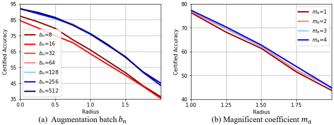
Here, we conducted detailed ablation studies to investigate the effectiveness of each component. We performed experiments on MNIST with $\sigma=1.0$ , and the results are shown in Figure 3. (More results are shown in the Appendix.) We investigated the influence by the augmentation batch size $b_{n}$ (Figure 3(a)) following the batch optimal transport setting. Also, we studied data augmentation sample size $m_{a}$ (Figure 3(b)). We found that a larger augmentation batch size $b_{n}$ leads to better performance, which is expected since it better approximates the joint measure. In addition, more augmented data samples $m_{a}$ benefit robustness, which agrees with our theoretical results.

6 Conclusion and Future Work

In this report, we proposed to characterize the robustness of a model through its performance on the Wasserstein geodesic connecting different training data distributions. The worst-case distributions on the geodesic allow us to create augmented data for training a more robust model. Further, we can regularize the smoothness of a classifier to promote robustness. We provided theoretical guarantees and carried out extensive experimental studies on multiple datasets, including CIFAR100 and ImageNet. Our results showed new SOTA performance compared with existing methods and can be easily combined with other learning schemes to boost the robustness.

As a first step, this work provides a new perspective to characterize the model’s robustness. There could be several future works, including considering multi-marginal adversarial Wasserstein barycenter on a simplex, more efficient optimization on the geodesic, and more thorough theoretical studies beyond Gaussian models.

References

Agueh & Carlier (2011) Martial Agueh and Guillaume Carlier. Barycenters in the wasserstein space. SIAM Journal on Mathematical Analysis, 43(2):904–924, 2011.
Albergo & Vanden-Eijnden (2022) Michael S Albergo and Eric Vanden-Eijnden. Building normalizing flows with stochastic interpolants. arXiv preprint arXiv:2209.15571, 2022.
Alvarez-Melis & Fusi (2020) David Alvarez-Melis and Nicolo Fusi. Geometric dataset distances via optimal transport. Advances in Neural Information Processing Systems, 33:21428–21439, 2020.
Alvarez-Melis & Fusi (2021) David Alvarez-Melis and Nicolò Fusi. Dataset dynamics via gradient flows in probability space. In International Conference on Machine Learning, pp. 219–230. PMLR, 2021.
Ambrosio et al. (2005) Luigi Ambrosio, Nicola Gigli, and Giuseppe Savaré. Gradient flows: in metric spaces and in the space of probability measures. Springer Science & Business Media, 2005.
Amos (2022) Brandon Amos. On amortizing convex conjugates for optimal transport. arXiv preprint arXiv:2210.12153, 2022.
Arjovsky et al. (2017) Martin Arjovsky, Soumith Chintala, and Léon Bottou. Wasserstein generative adversarial networks. In International conference on machine learning, pp. 214–223. PMLR, 2017.
Bahdanau et al. (2014) Dzmitry Bahdanau, Kyunghyun Cho, and Yoshua Bengio. Neural machine translation by jointly learning to align and translate. arXiv preprint arXiv:1409.0473, 2014.
Bhagoji et al. (2019) Arjun Nitin Bhagoji, Daniel Cullina, and Prateek Mittal. Lower bounds on adversarial robustness from optimal transport. arXiv preprint arXiv:1909.12272, 2019.
Brenier (1991) Yann Brenier. Polar factorization and monotone rearrangement of vector-valued functions. Communications on pure and applied mathematics, 44(4):375–417, 1991.
Bunne et al. (2022) Charlotte Bunne, Andreas Krause, and Marco Cuturi. Supervised training of conditional monge maps. arXiv preprint arXiv:2206.14262, 2022.
Cao et al. (2022) Chengtai Cao, Fan Zhou, Yurou Dai, and Jianping Wang. A survey of mix-based data augmentation: Taxonomy, methods, applications, and explainability. arXiv preprint arXiv:2212.10888, 2022.
Carlini & Wagner (2017) Nicholas Carlini and David Wagner. Towards evaluating the robustness of neural networks. In IEEE Symposium on Security and Privacy, pp. 39–57. IEEE, 2017.
Carmon et al. (2019) Yair Carmon, Aditi Raghunathan, Ludwig Schmidt, John C Duchi, and Percy S Liang. Unlabeled data improves adversarial robustness. Advances in Neural Information Processing Systems, 32, 2019.
Chrabaszcz et al. (2017) Patryk Chrabaszcz, Ilya Loshchilov, and Frank Hutter. A downsampled variant of imagenet as an alternative to the cifar datasets. arXiv preprint arXiv:1707.08819, 2017.
Cohen et al. (2019) Jeremy Cohen, Elan Rosenfeld, and Zico Kolter. Certified adversarial robustness via randomized smoothing. In International Conference on Machine Learning, pp. 1310–1320. PMLR, 2019.
Courty et al. (2017a) Nicolas Courty, Rémi Flamary, and Mélanie Ducoffe. Learning wasserstein embeddings. arXiv preprint arXiv:1710.07457, 2017a.
Courty et al. (2017b) Nicolas Courty, Rémi Flamary, Amaury Habrard, and Alain Rakotomamonjy. Joint distribution optimal transportation for domain adaptation. Advances in neural information processing systems, 30, 2017b.
Cuturi (2013) Marco Cuturi. Sinkhorn distances: Lightspeed computation of optimal transport. Advances in neural information processing systems, 26:2292–2300, 2013.
Dan et al. (2020) Chen Dan, Yuting Wei, and Pradeep Ravikumar. Sharp statistical guaratees for adversarially robust gaussian classification. In International Conference on Machine Learning, pp. 2345–2355. PMLR, 2020.
Deng et al. (2009) Jia Deng, Wei Dong, Richard Socher, Li-Jia Li, Kai Li, and Li Fei-Fei. Imagenet: A large-scale hierarchical image database. In 2009 IEEE conference on computer vision and pattern recognition, pp. 248–255. Ieee, 2009.
Deng et al. (2021) Zhun Deng, Linjun Zhang, Amirata Ghorbani, and James Zou. Improving adversarial robustness via unlabeled out-of-domain data. In International Conference on Artificial Intelligence and Statistics, pp. 2845–2853. PMLR, 2021.
Dong et al. (2020) Yinpeng Dong, Zhijie Deng, Tianyu Pang, Jun Zhu, and Hang Su. Adversarial distributional training for robust deep learning. Advances in Neural Information Processing Systems, 33:8270–8283, 2020.
Dowson & Landau (1982) DC Dowson and BV666017 Landau. The fréchet distance between multivariate normal distributions. Journal of multivariate analysis, 12(3):450–455, 1982.
Duchi & Namkoong (2021) John C Duchi and Hongseok Namkoong. Learning models with uniform performance via distributionally robust optimization. The Annals of Statistics, 49(3):1378–1406, 2021.
Fan & Alvarez-Melis (2022) Jiaojiao Fan and David Alvarez-Melis. Generating synthetic datasets by interpolating along generalized geodesics. In NeurIPS 2022 Workshop on Synthetic Data for Empowering ML Research, 2022.
Fan et al. (2020) Jiaojiao Fan, Amirhossein Taghvaei, and Yongxin Chen. Scalable computations of wasserstein barycenter via input convex neural networks. arXiv preprint arXiv:2007.04462, 2020.
Fan et al. (2021) Jiaojiao Fan, Shu Liu, Shaojun Ma, Yongxin Chen, and Haomin Zhou. Scalable computation of monge maps with general costs. arXiv preprint arXiv:2106.03812, pp. 4, 2021.
Fatras et al. (2019) Kilian Fatras, Younes Zine, Rémi Flamary, Rémi Gribonval, and Nicolas Courty. Learning with minibatch wasserstein: asymptotic and gradient properties. arXiv preprint arXiv:1910.04091, 2019.
Fatras et al. (2021a) Kilian Fatras, Thibault Séjourné, Rémi Flamary, and Nicolas Courty. Unbalanced minibatch optimal transport; applications to domain adaptation. In International Conference on Machine Learning, pp. 3186–3197. PMLR, 2021a.
Fatras et al. (2021b) Kilian Fatras, Younes Zine, Szymon Majewski, Rémi Flamary, Rémi Gribonval, and Nicolas Courty. Minibatch optimal transport distances; analysis and applications. arXiv preprint arXiv:2101.01792, 2021b.
Fisher (1936) Ronald A Fisher. The use of multiple measurements in taxonomic problems. Annals of eugenics, 7(2):179–188, 1936.
Gao & Chaudhari (2021) Yansong Gao and Pratik Chaudhari. An information-geometric distance on the space of tasks. In International Conference on Machine Learning, pp. 3553–3563. PMLR, 2021.
Givens & Shortt (1984) Clark R Givens and Rae Michael Shortt. A class of wasserstein metrics for probability distributions. Michigan Mathematical Journal, 31(2):231–240, 1984.
Goodfellow et al. (2020) Ian Goodfellow, Jean Pouget-Abadie, Mehdi Mirza, Bing Xu, David Warde-Farley, Sherjil Ozair, Aaron Courville, and Yoshua Bengio. Generative adversarial networks. Communications of the ACM, 63(11):139–144, 2020.
Goodfellow et al. (2014) Ian J Goodfellow, Jonathon Shlens, and Christian Szegedy. Explaining and harnessing adversarial examples. arXiv preprint arXiv:1412.6572, 2014.
Greenewald et al. (2021) Kristjan Greenewald, Anming Gu, Mikhail Yurochkin, Justin Solomon, and Edward Chien. k-mixup regularization for deep learning via optimal transport. arXiv preprint arXiv:2106.02933, 2021.
He & Sun (2015) Kaiming He and Jian Sun. Convolutional neural networks at constrained time cost. In Proceedings of the IEEE conference on computer vision and pattern recognition, pp. 5353–5360, 2015.
He et al. (2016) Kaiming He, X. Zhang, Shaoqing Ren, and Jian Sun. Deep residual learning for image recognition. 2016 IEEE Conference on Computer Vision and Pattern Recognition (CVPR), pp. 770–778, 2016.
Hendrycks et al. (2019) Dan Hendrycks, Norman Mu, Ekin D Cubuk, Barret Zoph, Justin Gilmer, and Balaji Lakshminarayanan. Augmix: A simple data processing method to improve robustness and uncertainty. arXiv preprint arXiv:1912.02781, 2019.
Hoffman et al. (2019) Judy Hoffman, Daniel A Roberts, and Sho Yaida. Robust learning with jacobian regularization. arXiv preprint arXiv:1908.02729, 2019.
Howard (2013) Andrew G Howard. Some improvements on deep convolutional neural network based image classification. arXiv preprint arXiv:1312.5402, 2013.
Hua et al. (2023) Xinru Hua, Truyen Nguyen, Tam Le, Jose Blanchet, and Viet Anh Nguyen. Dynamic flows on curved space generated by labeled data. arXiv preprint arXiv:2302.00061, 2023.
Huang et al. (2020) Chin-Wei Huang, Ricky TQ Chen, Christos Tsirigotis, and Aaron Courville. Convex potential flows: Universal probability distributions with optimal transport and convex optimization. arXiv preprint arXiv:2012.05942, 2020.
Huang et al. (2022) Peide Huang, Mengdi Xu, Jiacheng Zhu, Laixi Shi, Fei Fang, and Ding Zhao. Curriculum reinforcement learning using optimal transport via gradual domain adaptation. arXiv preprint arXiv:2210.10195, 2022.
Janati et al. (2020) Hicham Janati, Marco Cuturi, and Alexandre Gramfort. Debiased sinkhorn barycenters. In International Conference on Machine Learning, pp. 4692–4701. PMLR, 2020.
Jeong & Shin (2020) Jongheon Jeong and Jinwoo Shin. Consistency regularization for certified robustness of smoothed classifiers. In Advances in Neural Information Processing Systems, 2020.
Jeong et al. (2021) Jongheon Jeong, Sejun Park, Minkyu Kim, Heung-Chang Lee, Do-Guk Kim, and Jinwoo Shin. Smoothmix: Training confidence-calibrated smoothed classifiers for certified robustness. Advances in Neural Information Processing Systems, 34, 2021.
Kim et al. (2021a) Hoki Kim, Woojin Lee, Sungyoon Lee, and Jaewook Lee. Bridged adversarial training. arXiv preprint arXiv:2108.11135, 2021a.
Kim et al. (2020) Jang-Hyun Kim, Wonho Choo, and Hyun Oh Song. Puzzle mix: Exploiting saliency and local statistics for optimal mixup. In International Conference on Machine Learning, pp. 5275–5285. PMLR, 2020.
Kim et al. (2021b) Jang-Hyun Kim, Wonho Choo, Hosan Jeong, and Hyun Oh Song. Co-mixup: Saliency guided joint mixup with supermodular diversity. arXiv preprint arXiv:2102.03065, 2021b.
Kingma & Welling (2013) Diederik P Kingma and Max Welling. Auto-encoding variational bayes. arXiv preprint arXiv:1312.6114, 2013.
Knott & Smith (1984) Martin Knott and Cyril S Smith. On the optimal mapping of distributions. Journal of Optimization Theory and Applications, 43(1):39–49, 1984.
Korotin et al. (2022a) Alexander Korotin, Vage Egiazarian, Lingxiao Li, and Evgeny Burnaev. Wasserstein iterative networks for barycenter estimation. arXiv preprint arXiv:2201.12245, 2022a.
Korotin et al. (2022b) Alexander Korotin, Daniil Selikhanovych, and Evgeny Burnaev. Neural optimal transport. arXiv preprint arXiv:2201.12220, 2022b.
Krizhevsky (2009) Alex Krizhevsky. Learning multiple layers of features from tiny images. 2009.
Krizhevsky et al. (2017) Alex Krizhevsky, Ilya Sutskever, and Geoffrey E Hinton. Imagenet classification with deep convolutional neural networks. Communications of the ACM, 60(6):84–90, 2017.
Kurakin et al. (2016) Alexey Kurakin, Ian Goodfellow, and Samy Bengio. Adversarial machine learning at scale. arXiv preprint arXiv:1611.01236, 2016.
Le & Yang (2015) Ya Le and Xuan Yang. Tiny imagenet visual recognition challenge. CS 231N, 7(7):3, 2015.
LeCun et al. (1998) Yann LeCun, Léon Bottou, Yoshua Bengio, and Patrick Haffner. Gradient-based learning applied to document recognition. Proc. IEEE, 86:2278–2324, 1998.
Lewy & Mańdziuk (2022) Dominik Lewy and Jacek Mańdziuk. An overview of mixing augmentation methods and augmentation strategies. Artificial Intelligence Review, pp. 1–59, 2022.
Li et al. (2018) Bai Li, Changyou Chen, Wenlin Wang, and Lawrence Carin. Certified adversarial robustness with additive noise. arXiv preprint arXiv:1809.03113, 2018.
Li et al. (2021) Linyi Li, Maurice Weber, Xiaojun Xu, Luka Rimanic, Bhavya Kailkhura, Tao Xie, Ce Zhang, and Bo Li. Tss: Transformation-specific smoothing for robustness certification. In Proceedings of the 2021 ACM SIGSAC Conference on Computer and Communications Security, pp. 535–557, 2021.
Lin et al. (2022) Tianyi Lin, Nhat Ho, Marco Cuturi, and Michael I Jordan. On the complexity of approximating multimarginal optimal transport. Journal of Machine Learning Research, 23(65):1–43, 2022.
Liu et al. (2022) Xingchao Liu, Chengyue Gong, and Qiang Liu. Flow straight and fast: Learning to generate and transfer data with rectified flow. arXiv preprint arXiv:2209.03003, 2022.
Liutkus et al. (2019) Antoine Liutkus, Umut Simsekli, Szymon Majewski, Alain Durmus, and Fabian-Robert Stöter. Sliced-wasserstein flows: Nonparametric generative modeling via optimal transport and diffusions. In International Conference on Machine Learning, pp. 4104–4113. PMLR, 2019.
Madry et al. (2018) Aleksander Madry, Aleksandar Makelov, Ludwig Schmidt, Dimitris Tsipras, and Adrian Vladu. Towards deep learning models resistant to adversarial attacks. In International Conference on Learning Representations, 2018. URL https://openreview.net/forum?id=rJzIBfZAb.
Makkuva et al. (2020) Ashok Makkuva, Amirhossein Taghvaei, Sewoong Oh, and Jason Lee. Optimal transport mapping via input convex neural networks. In International Conference on Machine Learning, pp. 6672–6681. PMLR, 2020.
Manole et al. (2021) Tudor Manole, Sivaraman Balakrishnan, Jonathan Niles-Weed, and Larry Wasserman. Plugin estimation of smooth optimal transport maps. arXiv preprint arXiv:2107.12364, 2021.
McCann (1997) Robert J McCann. A convexity principle for interacting gases. Advances in mathematics, 128(1):153–179, 1997.
Moosavi-Dezfooli et al. (2019) Seyed-Mohsen Moosavi-Dezfooli, Alhussein Fawzi, Jonathan Uesato, and Pascal Frossard. Robustness via curvature regularization, and vice versa. In Proceedings of the IEEE/CVF Conference on Computer Vision and Pattern Recognition, pp. 9078–9086, 2019.
Mroueh & Nguyen (2021) Youssef Mroueh and Truyen Nguyen. On the convergence of gradient descent in gans: Mmd gan as a gradient flow. In International Conference on Artificial Intelligence and Statistics, pp. 1720–1728. PMLR, 2021.
Ng et al. (2020) Nathan Ng, Kyunghyun Cho, and Marzyeh Ghassemi. Ssmba: Self-supervised manifold based data augmentation for improving out-of-domain robustness. ArXiv, abs/2009.10195, 2020.
Nguyen et al. (2022) Khai Nguyen, Dang Nguyen, Tung Pham, Nhat Ho, et al. Improving mini-batch optimal transport via partial transportation. In International Conference on Machine Learning, pp. 16656–16690. PMLR, 2022.
Perrot et al. (2016) Michaël Perrot, Nicolas Courty, Rémi Flamary, and Amaury Habrard. Mapping estimation for discrete optimal transport. Advances in Neural Information Processing Systems, 29, 2016.
Pooladian & Niles-Weed (2021) Aram-Alexandre Pooladian and Jonathan Niles-Weed. Entropic estimation of optimal transport maps. arXiv preprint arXiv:2109.12004, 2021.
Qiu et al. (2022a) Jielin Qiu, Jiacheng Zhu, Michael Rosenberg, Emerson Liu, and Ding Zhao. Optimal transport based data augmentation for heart disease diagnosis and prediction. arXiv preprint arXiv:2202.00567, 2022a.
Qiu et al. (2022b) Jielin Qiu, Jiacheng Zhu, Mengdi Xu, Franck Dernoncourt, Trung Bui, Zhaowen Wang, Bo Li, Ding Zhao, and Hailin Jin. Semantics-consistent cross-domain summarization via optimal transport alignment. arXiv preprint arXiv:2210.04722, 2022b.
Radford et al. (2021) Alec Radford, Jong Wook Kim, Chris Hallacy, Aditya Ramesh, Gabriel Goh, Sandhini Agarwal, Girish Sastry, Amanda Askell, Pamela Mishkin, Jack Clark, Gretchen Krueger, and Ilya Sutskever. Learning transferable visual models from natural language supervision, 2021.
Ramesh et al. (2022) Aditya Ramesh, Prafulla Dhariwal, Alex Nichol, Casey Chu, and Mark Chen. Hierarchical text-conditional image generation with clip latents. arXiv preprint arXiv:2204.06125, 2022.
Rebuffi et al. (2021) Sylvestre-Alvise Rebuffi, Sven Gowal, Dan Andrei Calian, Florian Stimberg, Olivia Wiles, and Timothy A Mann. Data augmentation can improve robustness. Advances in Neural Information Processing Systems, 34, 2021.
Salman et al. (2019) Hadi Salman, Jerry Li, Ilya Razenshteyn, Pengchuan Zhang, Huan Zhang, Sebastien Bubeck, and Greg Yang. Provably robust deep learning via adversarially trained smoothed classifiers. Advances in Neural Information Processing Systems, 32, 2019.
Schmidt et al. (2018) Ludwig Schmidt, Shibani Santurkar, Dimitris Tsipras, Kunal Talwar, and Aleksander Madry. Adversarially robust generalization requires more data. arXiv preprint arXiv:1804.11285, 2018.
Seguy et al. (2017) Vivien Seguy, Bharath Bhushan Damodaran, Rémi Flamary, Nicolas Courty, Antoine Rolet, and Mathieu Blondel. Large-scale optimal transport and mapping estimation. arXiv preprint arXiv:1711.02283, 2017.
Sehwag et al. (2021) Vikash Sehwag, Saeed Mahloujifar, Tinashe Handina, Sihui Dai, Chong Xiang, Mung Chiang, and Prateek Mittal. Robust learning meets generative models: Can proxy distributions improve adversarial robustness? arXiv preprint arXiv:2104.09425, 2021.
Song & Ermon (2019) Yang Song and Stefano Ermon. Generative modeling by estimating gradients of the data distribution. Advances in Neural Information Processing Systems, 32, 2019.
Szegedy et al. (2014) Christian Szegedy, Wojciech Zaremba, Ilya Sutskever, Joan Bruna, D. Erhan, Ian J. Goodfellow, and Rob Fergus. Intriguing properties of neural networks. CoRR, abs/1312.6199, 2014.
Tokozume et al. (2017) Yuji Tokozume, Yoshitaka Ushiku, and Tatsuya Harada. Learning from between-class examples for deep sound recognition. arXiv preprint arXiv:1711.10282, 2017.
Uddin et al. (2020) AFM Uddin, Mst Monira, Wheemyung Shin, TaeChoong Chung, Sung-Ho Bae, et al. Saliencymix: A saliency guided data augmentation strategy for better regularization. arXiv preprint arXiv:2006.01791, 2020.
Venkataramanan et al. (2022) Shashanka Venkataramanan, Ewa Kijak, laurent amsaleg, and Yannis Avrithis. Alignmix: Improving representations by interpolating aligned features, 2022. URL https://openreview.net/forum?id=jFlWZEv6dv.
Verma et al. (2019) Vikas Verma, Alex Lamb, Christopher Beckham, Amir Najafi, Ioannis Mitliagkas, David Lopez-Paz, and Yoshua Bengio. Manifold mixup: Better representations by interpolating hidden states. In International Conference on Machine Learning, pp. 6438–6447. PMLR, 2019.
Villani (2009) Cédric Villani. Optimal transport: old and new, volume 338. Springer, 2009.
Volpi et al. (2018) Riccardo Volpi, Hongseok Namkoong, Ozan Sener, John C Duchi, Vittorio Murino, and Silvio Savarese. Generalizing to unseen domains via adversarial data augmentation. Advances in neural information processing systems, 31, 2018.
Wang et al. (2022) Haoxiang Wang, Bo Li, and Han Zhao. Understanding gradual domain adaptation: Improved analysis, optimal path and beyond. In International Conference on Machine Learning, pp. 22784–22801. PMLR, 2022.
Weber et al. (2022) Maurice Weber, Linyi Li, Boxin Wang, Zhikuan Zhao, Bo Li, and Ce Zhang. Certifying out-of-domain generalization for blackbox functions. arXiv preprint arXiv:2202.01679, 2022.
Wei et al. (2020) Colin Wei, Kendrick Shen, Yining Chen, and Tengyu Ma. Theoretical analysis of self-training with deep networks on unlabeled data. arXiv preprint arXiv:2010.03622, 2020.
Xiao et al. (2019) Chang Xiao, Peilin Zhong, and Changxi Zheng. Enhancing adversarial defense by k-winners-take-all. arXiv preprint arXiv:1905.10510, 2019.
Xing et al. (2022) Yue Xing, Qifan Song, and Guang Cheng. Unlabeled data help: Minimax analysis and adversarial robustness. In International Conference on Artificial Intelligence and Statistics, pp. 136–168. PMLR, 2022.
Yao et al. (2021) Huaxiu Yao, Linjun Zhang, and Chelsea Finn. Meta-learning with fewer tasks through task interpolation. arXiv preprint arXiv:2106.02695, 2021.
Yao et al. (2022) Huaxiu Yao, Yu Wang, Sai Li, Linjun Zhang, Weixin Liang, James Zou, and Chelsea Finn. Improving out-of-distribution robustness via selective augmentation. In International Conference on Machine Learning, pp. 25407–25437. PMLR, 2022.
Yun et al. (2019) Sangdoo Yun, Dongyoon Han, Seong Joon Oh, Sanghyuk Chun, Junsuk Choe, and Youngjoon Yoo. CutMix: Regularization strategy to train strong classifiers with localizable features. In Proceedings of the IEEE/CVF International Conference on Computer Vision, pp. 6023–6032, 2019.
Zhai et al. (2019) Runtian Zhai, Tianle Cai, Di He, Chen Dan, Kun He, John Hopcroft, and Liwei Wang. Adversarially robust generalization just requires more unlabeled data. arXiv preprint arXiv:1906.00555, 2019.
Zhai et al. (2020) Runtian Zhai, Chen Dan, Di He, Huan Zhang, Boqing Gong, Pradeep Ravikumar, Cho-Jui Hsieh, and Liwei Wang. MACER: Attack-free and scalable robust training via maximizing certified radius. In International Conference on Learning Representations, 2020.
Zhang & Wang (2019) Haichao Zhang and Jianyu Wang. Defense against adversarial attacks using feature scattering-based adversarial training. Advances in Neural Information Processing Systems, 32, 2019.
Zhang et al. (2018) Hongyi Zhang, Moustapha Cisse, Yann N. Dauphin, and David Lopez-Paz. mixup: Beyond empirical risk minimization. In International Conference on Learning Representations, 2018. URL https://openreview.net/forum?id=r1Ddp1-Rb.
Zhang et al. (2021) Linjun Zhang, Zhun Deng, Kenji Kawaguchi, Amirata Ghorbani, and James Zou. How does mixup help with robustness and generalization? In International Conference on Learning Representations, 2021. URL https://openreview.net/forum?id=8yKEo06dKNo.
Zhang et al. (2022) Linjun Zhang, Zhun Deng, Kenji Kawaguchi, and James Zou. When and how mixup improves calibration. In International Conference on Machine Learning, pp. 26135–26160. PMLR, 2022.
Zhu et al. (2021) Jiacheng Zhu, Aritra Guha, Dat Do, Mengdi Xu, XuanLong Nguyen, and Ding Zhao. Functional optimal transport: map estimation and domain adaptation for functional data, 2021.
Zhu et al. (2022a) Jiacheng Zhu, Gregory Darnell, Agni Kumar, Ding Zhao, Bo Li, Xuanlong Nguyen, and Shirley You Ren. Physiomtl: Personalizing physiological patterns using optimal transport multi-task regression. arXiv preprint arXiv:2203.12595, 2022a.
Zhu et al. (2022b) Jiacheng Zhu, Jielin Qiu, Zhuolin Yang, Douglas Weber, Michael A Rosenberg, Emerson Liu, Bo Li, and Ding Zhao. Geoecg: Data augmentation via wasserstein geodesic perturbation for robust electrocardiogram prediction. arXiv preprint arXiv:2208.01220, 2022b.
Zhu et al. (2020) Jianchao Zhu, Liangliang Shi, Junchi Yan, and Hongyuan Zha. Automix: Mixup networks for sample interpolation via cooperative barycenter learning. In European Conference on Computer Vision, pp. 633–649. Springer, 2020.

Appendix

\parttoc

Appendix A Theoretical results

A.1 The Wasserstein distance between Gaussian distribution

Theorem A.1 (The Wasserstein distance between Gaussian distribution ).

Given two Gaussian measures, $P^{0}=N(\mu_{0},\Sigma_{0})$ and $P^{1}=N(\mu_{1},\Sigma_{1})$ . The $L^{2}$ -Wasserstein distance between them is given by

	$\displaystyle W^{2}_{2}(P^{0},P^{1})=$	$\displaystyle\\|\mu_{0}-\mu_{1}\\|^{2}+tr(\Sigma_{0})+tr(\Sigma_{1})$		(18)
		$\displaystyle-2tr(\sqrt{\Sigma_{0}^{1/2}\Sigma_{1}\Sigma_{0}^{1/2}})$		(18)

The proof largely depends on a summary of Givens & Shortt (1984), as well as. We recall the theorem. Given two Gaussian measures, $P^{0}=N(\mu_{0},\Sigma_{0})$ and $P^{1}=N(\mu_{1},\Sigma_{1})$ . The $L^{2}$ -Wasserstein distance between them is given by

\displaystyle W^{2}_{2}(P^{0},P^{1})=

\displaystyle\|\mu_{0}-\mu_{1}\|^{2}+tr(\Sigma_{0})+tr(\Sigma_{1})-2tr(\sqrt{\Sigma_{0}^{1/2}\Sigma_{1}\Sigma_{0}^{1/2}})

(19)

Given two distributions $P^{0}=N(\mu_{0},\Sigma_{0})$ and $P^{1}=N(\mu_{1},\Sigma_{1})$ , one can first reduce to the centered case $\mu_{0}=\mu_{1}=0$ . Next, let $X\sim P^{0}$ and $Y\sim P^{1}$ and if $(X,Y)$ is a random vector of $\mathbb{R}^{n}\times\mathbb{R}^{n}$ with covariance matrix

\Gamma=\begin{bmatrix}\Sigma_{0}&C\\ C^{\top}&\Sigma_{1}\end{bmatrix}

then the quantity

\mathbb{E}[\|X-Y\|^{2}_{2}]=Tr(\Sigma_{0}+\Sigma_{1}-2C)

depends only on $\Gamma$ . Also, when $P^{0}=N(0,\Sigma_{0})$ and $P^{1}=N(0,\Sigma_{1})$ , one can restrict the infimum which defines $W_{2}$ to run over $W_{2}$ to run over Gaussian laws $N(0,\Gamma)$ on $\mathbb{R}^{n}\times\mathbb{R}^{n}$ with covariance matrix $\Gamma$ structured above. Here the constrain on $C$ is the Schur complement constraint $\Sigma_{0}-C\Sigma^{-1}_{1}C^{\top}\succeq 0.$ Thus, the minimization of the function $C\mapsto-2Tr(C)$ leads to the result.

A.2 Transport map between Gaussian measures

Proposition A.2 (Optimal transport map between Gaussian measures, adopted from Knott & Smith (1984), Example 1.7 McCann (1997)).

Given the two Gaussian distributions defined in theorem (18), define a symmetric positive matrix $T$ and a corresponding linear map $\mathcal{T}:\mathcal{X}\mapsto\mathcal{X}$

	$\displaystyle\mathcal{T}(x)=\mu_{1}+T(x-\mu_{0}),{{}where}$		(20)
	$\displaystyle T=\Sigma_{1}^{1/2}(\Sigma_{1}^{1/2}\Sigma_{0}\Sigma_{1}^{1/2})^{-1/2}\Sigma_{1}^{1/2}$		(20)

Then, $\mathcal{T}$ is the optimal map such that $P^{1}=T\#P^{0}$ .

Hence we obtain a closed-form map and that leads to an explicit form of the geodesic interpolation among two Gaussian distributions, as:

\displaystyle{T}^{G,xy}_{t}:=\begin{cases}{T}^{G,x}_{t}(x^{0})&=(1-t)x^{0}+\mathcal{T}(x^{0}),\\ {T}^{G,y}_{t}(y^{0})&=\begin{cases}y^{0},{{}}0<t<0.5,\\ -y^{0},{{}}0.5<t<1.\end{cases}\end{cases}

Here the interpolation of $y^{0}$ means we will always label a sample as $-1$ or $1$ , which allows us to proceed to the analysis under the classification error. Given the two Gaussian distributions defined in theorem (18), define a symmetric positive matrix $T$ and a corresponding linear map $\mathcal{T}:\mathcal{X}\mapsto\mathcal{X}$

	$\displaystyle\mathcal{T}(x)=\mu_{1}+T(x-\mu_{0}),{{}where}$
	$\displaystyle T=\Sigma_{1}^{1/2}(\Sigma_{1}^{1/2}\Sigma_{0}\Sigma_{1}^{1/2})^{-1/2}\Sigma_{1}^{1/2}$

Then, $\mathcal{T}$ is the optimal map such that $P^{1}=T\#P^{0}$ .

Check the optimal transport map from $N(\mu_{0},\Sigma_{0})$ to $N(\mu_{1},\Sigma_{1})$ , again assume $\mu_{0}=\mu_{1}=0$ for simplicity, one may define the random column vectors $X\sim N(\mu_{0},\Sigma_{1})$ and $Y=TX$ and write

	$\displaystyle\mathbb{E}(YY^{\top})$	$\displaystyle=T\mathbb{E}(XX^{\top})T^{\top}$
		$\displaystyle=\Sigma_{0}^{-1/2}(\Sigma^{1/2}_{1}\Sigma_{2}\Sigma^{1/2}_{0})^{1/2}(\Sigma^{1/2}_{1}\Sigma_{2}\Sigma^{1/2}_{0})^{1/2}\Sigma_{0}^{-1/2}$
		$\displaystyle=\Sigma_{1}$

To show the map is optimal, one may use

	$\displaystyle\mathbb{E}(\\|X-Y\\|^{2}_{2})$	$\displaystyle=\mathbb{E}(\\|X\\|^{2}_{2})+\mathbb{E}(\\|Y\\|^{2}_{2})-2\mathbb{E}(<X,Y>)$
		$\displaystyle=Tr(\Sigma_{0})+Tr(\Sigma_{1})-2\mathbb{E}(<X,TX>)$
		$\displaystyle=Tr(\Sigma_{0})+Tr(\Sigma_{1})-2Tr(\Sigma_{0}T)$

and one can observe that by the cyclic property of the trace

Tr(\Sigma_{0}T)=Tr((\Sigma^{1/2}_{1}\Sigma_{2}\Sigma^{1/2}_{0})^{1/2})

Moreover, for the interpolation Geodesic, the following result holds.

Proposition A.3 (Interpolation between Gaussian distributions (McCann, 1997) example 1.7).

Given the two Gaussian distributions defined in theorem (18), respectively. A constant speed geodesic is defined by the the path $(G^{g}_{t})_{t\in[0,1]}$ , such that $\forall t\in[0,1]$ , and $G^{g}_{t}:=N(m_{t},\Sigma_{t})$ is given by

		$\displaystyle m_{t}=(1-t)\mu_{1}+t\mu_{2},$		(21)
		$\displaystyle\Sigma_{t}=((1-t)Id+tT)\Sigma_{1}((1-t)Id+tT)$		(21)

where $T=\Sigma_{1}^{1/2}(\Sigma_{1}^{1/2}\Sigma_{0}\Sigma_{1}^{1/2})^{-1/2}\Sigma_{1}^{1/2}$ .

We have illustrated that the Wasserstein barycenter, on the geodesic, of two Gaussian distributions is still a Gaussian distribution and admits an explicit form.

	where,	$\displaystyle T^{x}_{t}(x)=(1-t)x+tT^{x}(x),$		(22)
		$\displaystyle T^{y}_{t}(y)=(1-t)y+tT^{y}(y)$		(22)

A.3 The effect of the regularization

Recall that the geodesic regularization term is

\displaystyle\text{Reg}^{T^{xy}}_{l}(f_{\theta})=\int_{t=0}^{1}\left|\frac{d}{dt}\int_{\mathcal{X}\times\mathcal{Y}}l(f_{\theta}(T^{x}_{t}(x),T^{y}_{t}(y))dP^{0}(x,y)\right|dt

(23)

Recall the classifier to be $f_{\theta}(x)=\langle\theta,x\rangle=\theta^{\top}x$ , and the loss to be $l(f(x),y)=-yf(x)$ ,

Consider the following minimization problem

\min_{f\in\mathcal{H}}\mathbb{E}_{(x,y)\sim P_{all}}[l(f(x),y)]+\frac{\lambda_{1}}{2}\text{Reg}^{T^{xy}}_{l}(f_{\theta})

(24)

Proof. The problem above can be written as follows

\min_{\theta\in\mathbb{R}^{d}}\mathcal{L}(\theta)=-(\langle\theta,\mu_{1}-\mu_{0}\rangle)+\lambda_{1}\text{Reg}(\theta)

(25)

And under the above setting, we have

$\displaystyle\text{Reg}^{T^{xy}}_{l}(f_{\theta})$	$\displaystyle=\int_{t=0}^{1}\left\|\frac{d}{dt}\int_{\mathcal{X}\times\mathcal{Y}}l(f_{\theta}(T^{x}_{t}(x),T^{y}_{t}(y))dP^{0}(x,y)\right\|dt$	(26)
	$\displaystyle=\int_{t=0}^{1}\left\|\frac{d}{dt}\mathbb{E}_{x_{0}.y_{0}\sim P^{0}(x,y)}[l(f_{\theta}(T^{x}_{t}(x),T^{y}_{t}(y))]\right\|dt$
	$\displaystyle=\int_{t=0}^{1}\left\|\frac{d}{dt}\mathbb{E}_{x_{0}.y_{0}\sim P^{0}(x,y)}[-T^{y}_{t}(y_{0})\langle\theta,T^{x}_{t}(x_{0})\rangle]\right\|dt$
	Recall the parameterization of the map as interpolation, as e.q., 7,

Here, using the dominated convergence theorem. Also, use the closed form interpolation $T^{x}_{t}(x_{0})=(1-t)x_{0}+t\hat{T}(x_{0})$ , and $T^{y}_{t}(y_{0})=2t-1$ ( $y_{0}=-1$ and $y_{1}=1$ ), the above equation turns into

\displaystyle=\int_{t=0}^{1}\left|\mathbb{E}_{x_{0}.y_{0}\sim P^{0}(x,y)}[-2\langle\theta,T^{x}_{t}(x_{0})\rangle-(2t-1)\langle\theta,\hat{T}(x_{0})-x_{0}\rangle]\right|dt

(27)

Since we have closed-form expression for the geodesic as $\mathbb{E}_{x_{0}\sim P^{0}}[T^{t}(x_{0})]=(2t-1)\mu$ and $\mathbb{E}_{x_{0}\sim P^{0}}[\hat{T}(x_{0})-x_{0}]=2\mu$ , then

\displaystyle=\int_{t=0}^{1}\left|-2(2t-1)\theta^{\top}\mu-2(2t-1)\theta^{\top}\mu\right|dt=\int_{t=0}^{1}\left|4(1-2t)\theta^{\top}\mu\right|dt=2|\theta^{\top}\mu|

(28)

Then, the objective becomes

\min_{\theta}\mathcal{L}(\theta):=-\langle\theta,\mu\rangle+\frac{\lambda_{1}}{2}|\langle\theta,\mu\rangle|^{2}+\frac{\lambda_{2}}{2}\|\theta\|^{2}_{2}

(29)

Setting the first-order derivative to be zero, we obtain the solution

	$\displaystyle\nabla_{\theta}\mathcal{L}(\theta)$	$\displaystyle=-\mu+\lambda_{1}\mu\otimes\mu\theta+\lambda_{2}\theta=0,$		(30)
	$\displaystyle\theta^{*}$	$\displaystyle=(\lambda_{1}\mu\otimes\mu+\lambda_{2}I_{m})^{-1}\mu$		(30)

From Eq. (29), we can see that geodesic regularization is a data-adaptive regularization that smooths the classifier according to the distribution of original data.

A.4 Proof of Proposition 3.1

Assumptions and generalisation

Without loss of generalisation, we assume $\sigma=1$ and $\mu=(1,0,\ldots,0)$ , with $1$ at the first coordinate and $0$ elsewhere. Thus $\|\mu\|=1$ .

Since $\eta(x|y=-1),\eta(x|y=1)$ are both Gaussian, assume $\eta(x|y=-1)\sim N(\psi_{-1},\Sigma_{-1})$ and $\eta(x|y=1)\sim N(\psi_{1},\Sigma_{1})$ .

Let $u_{1},\ldots,u_{d}$ be the eigenvalues of $\Sigma_{0}$ Following Theorem A.1, we have

	$\displaystyle W^{2}_{2}(N_{d}(\psi_{1},\Sigma_{1}),N_{d}(\mu,\mathbb{I}))$	$\displaystyle=\\|\psi_{1}-\mu\\|^{2}+tr(\Sigma_{1})+d-2tr({\Sigma_{1}}^{1/2})$		(31)
		$\displaystyle=\\|\psi_{1}-\mu\\|^{2}+\sum_{i=1}^{d}\left(\sqrt{u_{i}}-1\right)^{2}$		(31)

Similarly,

\displaystyle W^{2}_{2}(N_{d}(\psi_{-1},\Sigma_{-1}),N_{d}(-\mu,\mathbb{I}))=\|\psi_{-1}+\mu\|^{2}+\sum_{i=1}^{d}\left(\sqrt{v_{i}}-1\right)^{2},

(32)

where $\{v_{i}\}_{1}^{d}$ are the eigenvalues of $\Sigma_{-1}$ .

By linearity property of Gaussian distributions $\eta(X|Y=y)\sim N(\psi_{y},\Sigma_{y})$ implies, $\alpha^{\prime}X+\beta|Y=y\sim N(\alpha^{\prime}\psi_{y}+\beta,\alpha^{\prime}\Sigma_{y}\alpha)$ . Therefore,

\displaystyle\mathbb{E}_{(X,Y)\sim\eta(X|Y)\nu(Y)}l(f_{(\alpha,\beta)}(X),Y)\propto P_{N(0,1)}\left(Z_{1}<-\dfrac{(\alpha^{\prime}\psi_{1}+\beta)}{\sqrt{\alpha^{\prime}\Sigma_{1}\alpha}}\right)+P_{N(0,1)}\left(Z_{-1}>-\dfrac{(\alpha^{\prime}\psi_{-1}+\beta)}{\sqrt{\alpha^{\prime}\Sigma_{-1}\alpha}}\right),

(33)

where $Z_{1}=\dfrac{\alpha^{\prime}(X-\psi_{1})}{\sqrt{\alpha^{\prime}\Sigma_{1}\alpha}}\biggr{|}Y=1\sim N(0,1)$ if $X|Y=1\sim N(\psi_{1},\Sigma_{1})$ and
$Z_{-1}=\dfrac{\alpha^{\prime}(X-\psi_{-1})}{\sqrt{\alpha^{\prime}\Sigma_{-1}\alpha}}\biggr{|}Y=-1\sim N(0,1)$ if $X|Y=-1\sim N(\psi_{-1},\Sigma_{-1})$ .

The LHS of Eq. (5) becomes

\displaystyle\max_{(\psi_{1},\psi_{-1},\Sigma_{1},\Sigma_{-1})\in B_{\epsilon}(\mu)}\inf_{\alpha,\beta}P_{N(0,1)}\left(Z_{1}<-\dfrac{(\alpha^{\prime}\psi_{1}+\beta)}{\sqrt{\alpha^{\prime}\Sigma_{1}\alpha}}\right)+P_{N(0,1)}\left(Z_{-1}>-\dfrac{(\alpha^{\prime}\psi_{-1}+\beta)}{\sqrt{\alpha^{\prime}\Sigma_{-1}\alpha}}\right),

(34)

where, $B_{\epsilon}(\mu)=\{(\psi_{1},\psi_{-1},\Sigma_{1},\Sigma_{-1}):\|\psi_{-1}+\mu\|^{2}+\sum_{i=1}^{d}\left(\sqrt{v_{i}}-1\right)^{2}\leq\epsilon^{2},\|\psi_{1}-\mu\|^{2}+\sum_{i=1}^{d}\left(\sqrt{u_{i}}-1\right)^{2}\leq\epsilon^{2}\}$ $\{u_{i}\}_{1}^{d}$ are eigenvalues of $\Sigma_{-1}$ , and $\{u_{i}\}_{1}^{d}$ are eigenvalues of $\Sigma_{-1}$ .

Step 1:

First, we show the proof under the assumption $\Sigma_{1}=\Sigma_{-1}=\Sigma$ .

Fixing $\psi_{1},\psi_{-1},\Sigma$ so that $\psi_{1},\psi_{-1},\Sigma,\Sigma\in B_{\epsilon}(\mu)$ and setting derivative to $0$ of

\displaystyle P_{N(0,1)}\left(Z_{1}<-\dfrac{(\alpha^{\prime}\psi_{1}+\beta)}{\sqrt{\alpha^{\prime}\Sigma\alpha}}\right)+P_{N(0,1)}\left(Z_{-1}>-\dfrac{(\alpha^{\prime}\psi_{-1}+\beta)}{\sqrt{\alpha^{\prime}\Sigma\alpha}}\right)

(35)

w.r.t $\beta$ yields either (i) $\alpha^{\prime}\psi_{1}+\beta=\alpha^{\prime}\psi_{-1}+\beta$ , or (ii) $\alpha^{\prime}\psi_{1}+\beta=-(\alpha^{\prime}\psi_{-1}+\beta)$ .

Setting derivative of (35) w.r.t $\alpha$ to $0$ yields $\psi_{1}=\psi_{-1}$ , which clearly is a contradiction for $\epsilon<1$ .

Considering (ii) above yields $\beta=-\alpha^{\prime}(\psi_{-1}+\psi_{1})/2$ . Then Eq. (35) leads to

	$\displaystyle P_{N(0,1)}\left(Z>\dfrac{\alpha^{\prime}(\psi_{1}-\psi_{-1})}{2\sqrt{\alpha^{\prime}\Sigma\alpha}}\right)+P_{N(0,1)}\left(Z<-\dfrac{\alpha^{\prime}(\psi_{1}-\psi_{-1})}{2\sqrt{\alpha^{\prime}\Sigma\alpha}}\right)$
	$\displaystyle=2P_{N(0,1)}\left(Z>\dfrac{\alpha^{\prime}(\psi_{1}-\psi_{-1})}{2\sqrt{\alpha^{\prime}\Sigma\alpha}}\right).$		(36)

The RHS above is minimized w.r.t $\alpha$ when $\dfrac{\alpha^{\prime}(\psi_{1}-\psi_{-1})}{2\sqrt{\alpha^{\prime}\Sigma\alpha}}$ is maximized. A simple calculation shows that this is achieved for $\alpha=\dfrac{\tilde{a}\Sigma^{-1}}{\sqrt{\tilde{a}^{\prime}\Sigma^{-1}\tilde{a}}}$ , where $\tilde{a}=(\psi_{1}-\psi_{-1})$ . This gives $\dfrac{\alpha^{\prime}(\psi_{1}-\psi_{-1})}{\sqrt{\alpha^{\prime}\Sigma\alpha}}={\sqrt{\tilde{a}^{\prime}\Sigma^{-1}\tilde{a}}}$ .

For a given $\Sigma$ , this is minimized (and equivalently Eq. (35) is maximised) when $(\psi_{1}-\psi_{-1})/2$ is in the direction of the largest eigenvector of $\Sigma$ , say $v_{1}$ , and $\tilde{a}^{\prime}\Sigma^{-1}\tilde{a}=\|\psi_{1}-\psi_{-1}\|^{2}/v_{1}$ .

Notice that since the other eigenvalues do not affect the choice of $(\psi_{1}-\psi_{-1})$ , based on the constraints $\|\psi_{-1}+\mu\|^{2}+\sum_{i=1}^{d}\left(\sqrt{v_{i}}-1\right)^{2}\leq\epsilon^{2}$ and $\|\psi_{1}+\mu\|^{2}+\sum_{i=1}^{d}\left(\sqrt{v_{i}}-1\right)^{2}\leq\epsilon^{2}$ , where $v_{i}$ are the ordered eigenvalues of $\Sigma$ , we can assume all other eigenvalues to be $1$ without affecting the value in the RHS of Eq. (A.4).

Let the largest eigenvalue of $\Sigma$ be $(1+\delta)^{2}$ . Then based on the constraints $\|\psi_{1}-\psi_{-1}\|^{2}/v_{1}$ is minimized when $\psi_{1}=-\psi_{-1}$ and they are concurrent with $\mu$ and $-\mu$ .

Based on the constraints, this yields,

\displaystyle\sqrt{\|\psi_{1}-\psi_{-1}\|^{2}/v_{1}}=2(1-\sqrt{\epsilon^{2}-\delta^{2}})/(1+\delta),

(37)

which is an increasing function of $\delta$ and is minimised at $\delta=1$ , which implies $\Sigma=\mathbb{I}$ , and $\psi_{1}=(1-\epsilon)\mu$ , $\psi_{-1}=(1-\epsilon)-\mu$ , which are the geodesic optimizers.

Therefore,

	$\displaystyle\max_{\tilde{A}(\nu_{\mu},\epsilon)}\inf_{\alpha,\beta}\mathbb{E}_{(X,Y)\sim\eta(X\|Y)\nu(Y)}l(f_{(\alpha,\beta)}(X),Y)=$
	$\displaystyle\mathbb{E}_{(X,Y)\sim\nu_{(1-\epsilon)\mu}(X\|Y)\nu(Y)}l(f_{(\mu,0)}(X),Y).$		(38)

where $\tilde{A}(\nu_{\mu},\epsilon)=\{\eta(X|Y):\eta(\cdot|Y)$ is Gaussian, $W(\eta(X|Y),\nu_{\mu}(X|Y))\leq\epsilon,\ \forall Y\in\{-1,1\}$ , $Cov(\eta(\cdot|Y=1))=Cov(\eta(\cdot|Y=-1))\}$

Step 2:

Next, we use the result in Step 1 to show the remaining.

Therefore, consider the situation where we do not restrict to $\Sigma_{1}=\Sigma_{-1}$ .

Set $\Sigma^{0}_{1}=\Sigma^{0}_{-1}=\mathbb{I}$ , $\psi^{0}_{1}=(1-\epsilon)\mu$ , $\psi^{0}_{-1}=-(1-\epsilon)\mu$ , $\alpha_{0}=(1-\epsilon)\mu$ , $\beta_{0}=0$ . Also, let

\displaystyle F(\psi_{1},\psi_{-1},\Sigma_{1},\Sigma_{-1},\alpha,\beta):=\mathbb{E}_{(X,Y)\sim\eta(X|Y)\nu(Y)}l(f_{(\alpha,\beta)}(X),Y),

(39)

where $\eta(X|Y=1)\sim N(\psi_{1},\Sigma_{1})$ , $\eta(X|Y=-1)\sim N(\psi_{-1},\Sigma_{-1})$ .

Note that $F(\psi^{0}_{1},\psi^{0}_{-1},\Sigma^{0}_{1},\Sigma^{0}_{-1},\alpha_{0},\beta_{0})={E}_{(X,Y)\sim\nu_{(1-\epsilon)\mu}(X|Y)\nu(Y)}l(f_{(\mu,0)}(X),Y)$ .

From Step 1 of the proof, we have shown that, $F(\psi^{0}_{1},\psi^{0}_{-1},\Sigma^{0}_{1},\Sigma^{0}_{-1},\alpha,\beta)\geq F(\psi^{0}_{1},\psi^{0}_{-1},\Sigma^{0}_{1},\Sigma^{0}_{-1},\alpha_{0},\beta_{0})$ .

Now, we claim it is enough to show $F(\psi_{1},\psi_{-1},\Sigma_{1},\Sigma_{-1},\alpha_{0},\beta_{0})\leq F(\psi^{0}_{1},\psi^{0}_{-1},\Sigma^{0}_{1},\Sigma^{0}_{-1},\alpha_{0},\beta_{0})$ for $\psi_{1},\psi_{-1},\Sigma_{1},\Sigma_{-1}\in{A}(\nu_{\mu},\epsilon)$ , since then

	$\displaystyle\max_{\tilde{A}(\nu_{\mu},\epsilon)}inf_{\alpha,\beta}F(\psi^{0}_{1},\psi^{0}_{-1},\Sigma^{0}_{1},\Sigma^{0}_{-1},\alpha,\beta)$	(40)
$\displaystyle\geq$	$\displaystyle inf_{\alpha,\beta}F(\psi^{0}_{1},\psi^{0}_{-1},\Sigma^{0}_{1},\Sigma^{0}_{-1},\alpha,\beta)$
$\displaystyle\geq$	$\displaystyle F(\psi^{0}_{1},\psi^{0}_{-1},\Sigma^{0}_{1},\Sigma^{0}_{-1},\alpha_{0},\beta_{0})$
$\displaystyle\geq$	$\displaystyle\max_{\tilde{A}(\nu_{\mu},\epsilon)}F(\psi_{1},\psi_{-1},\Sigma_{1},\Sigma_{-1},\alpha_{0},\beta_{0})$
$\displaystyle\geq$	$\displaystyle inf_{\alpha,\beta}\max_{\tilde{A}(\nu_{\mu},\epsilon)}F(\psi^{0}_{1},\psi^{0}_{-1},\Sigma^{0}_{1},\Sigma^{0}_{-1},\alpha,\beta)$

and we know that

\displaystyle inf_{\alpha,\beta}\max_{A(\nu_{\mu},\epsilon)}F(\psi^{0}_{1},\psi^{0}_{-1},\Sigma^{0}_{1},\Sigma^{0}_{-1},\alpha,\beta)\geq\max_{A(\nu_{\mu},\epsilon)}inf_{\alpha,\beta}F(\psi^{0}_{1},\psi^{0}_{-1},\Sigma^{0}_{1},\Sigma^{0}_{-1},\alpha,\beta)

(41)

This would imply that

	$\displaystyle inf_{\alpha,\beta}\max_{A(\nu_{\mu},\epsilon)}F(\psi^{0}_{1},\psi^{0}_{-1},\Sigma^{0}_{1},\Sigma^{0}_{-1},\alpha,\beta)$	$\displaystyle=$	$\displaystyle\max_{A(\nu_{\mu},\epsilon)}inf_{\alpha,\beta}F(\psi^{0}_{1},\psi^{0}_{-1},\Sigma^{0}_{1},\Sigma^{0}_{-1},\alpha,\beta)$		(42)
		$\displaystyle=$	$\displaystyle{E}_{(X,Y)\sim\nu_{(1-\epsilon)\mu}(X\|Y)\nu(Y)}l(f_{(\mu,0)}(X),Y)$		(42)

and complete the proof.

Now,

\displaystyle F(\psi_{1},\psi_{-1},\Sigma_{1},\Sigma_{-1},\alpha_{0},\beta_{0})=P\left(Z<\dfrac{\mu^{\prime}\psi_{-1}}{\sqrt{\mu^{\prime}\Sigma_{-1}\mu}}\right)+P\left(Z>\dfrac{\mu^{\prime}\psi_{1}}{\sqrt{\mu^{\prime}\Sigma_{-1}\mu}}\right).

(43)

Since the constraints in $A(\nu_{\mu},\epsilon)$ are separate and symmetric with respect to $\psi_{1},\Sigma_{1}$ and $\psi_{-1},\Sigma_{-1}$ respectively, and standard Normal distribution is symmetric. Therefore the max of $F(\psi_{1},\psi_{-1},\Sigma_{1},\Sigma_{-1},\alpha_{0},\beta_{0})$ over $A(\nu_{\mu},\epsilon)$ is attained when $\psi_{-1}=-\psi_{1}$ and $\Sigma_{1}=\Sigma_{-1}$ . The remainder follows from Step 1.

A.5 Error probabilities in closed form (Definition 4.2)

Standard accuracy probability.

The standard accuracy probability is given as

\mathbb{P}_{x\sim D}(f_{\theta}(x)=y)=1-\mathbb{P}_{x\sim D}(yx^{\top}\theta<0)=1-Q\left(\frac{\mu^{\top}\theta}{\sigma\|\theta\|}\right)

(44)

where $Q(x)=\frac{1}{\sqrt{2\pi}}\int^{\infty}_{x}e^{-t^{2}/2}dt$ .

$l_{\infty}^{\epsilon}$ robust accuracy.

The $l_{\infty}^{\epsilon}$ robust accuracy is given as:

	$\displaystyle\inf_{\\|v\\|_{\infty}<\epsilon}\mathbb{P}_{x\sim D}(f_{\theta}(x)=y)$	$\displaystyle=1-\mathbb{P}_{x\sim D}\left(\inf_{\\|v\\|_{\infty}<\epsilon}\left\{y\cdot(x+v)^{\top}\theta\right\}<0\right)$
		$\displaystyle=1-Q\left(\frac{\mu^{\top}\theta}{\sigma\\|\theta\\|}-\frac{\epsilon\\|\theta\\|_{1}}{\sigma\\|\theta\\|}\right)$		(45)

$l_{2}^{\sigma_{s}}$ smoothed classifier for certifiable robust accuracy.

It is the accuracy probability from a $N(0,\sigma_{s}^{2}I)$ smoothed classifier:

\displaystyle\mathbb{P}_{x\sim D,\delta\sim N(0,\sigma_{s}^{2}I)}(f_{\theta}(x+\delta)=y)

(46)

The above probability involves two random variables $x(y)\sim D$ and $\delta\sim N(0,\sigma_{s}^{2}I)$ , which are independent of each other. This addition is considered as the convolution of two pdfs. Since $D$ is a mixture of Gaussian and $\delta$ subjects to a Gaussian, there is a closed form

\displaystyle D^{*}=N(\mu,\sigma^{2}I)\ast N(0,\sigma_{s}^{2}I)=N(\mu,\sigma^{2}+\sigma_{s}^{2}I)

(47)

Thus, the certifiable robust accuracy in this setting is equivalent to the standard accuracy probability from a convoluted dataset.

\displaystyle\mathbb{P}_{x\sim D^{*}}(f_{\theta}(x)=y)=1-Q\left(\frac{\mu^{\top}\theta}{(\sigma+\sigma_{s})\|\theta\|}\right)

(48)

A.6 Provable improvement from data augmentation (Theorem 4.3)

Proof.

We divide the proof into several steps as follows:

Step 1:

The distribution of original data $(X,Y)$ is iid with $X|Y\sim N(y\mu,\sigma^{2}I)$ . Thus, from Eq.(10) and (11) in Carmon et al. (2019), we have

\displaystyle\mathbb{PE}^{p,\epsilon}_{a}(f_{\theta})=Q\left(\dfrac{\mu^{T}\theta}{\sigma\|\theta\|}-\dfrac{\epsilon\sqrt{d}}{\sigma}\right),~{}\text{where}~{}Q(x)=\dfrac{1}{2\pi}\int_{x}^{\infty}e^{-z^{2}/2}\mathrm{d}z.

(49)

Let $\alpha(n_{0},n_{1})$ be used to denote $n_{1}/(n_{0}+n_{1})$ . Additionally, let $\hat{{\theta}}_{n_{1}}=\dfrac{\left(\sum_{i=1}^{n_{1}}\tilde{Y}_{i}\tilde{X}_{i}\right)}{n_{1}}$ .

Step 2:

Note that $\mathbb{PE}^{p,\epsilon}_{a}(f_{\hat{\theta}_{n_{0}}})\geq\mathbb{PE}^{p,\epsilon}_{a}(f_{\hat{\theta}_{n_{0},n_{1}}})$ holds as long as $\dfrac{\mu^{T}\hat{\theta}_{n_{0}}}{\|\mu\|\|\hat{\theta}_{n_{0}}\|}\leq\dfrac{\mu^{T}\hat{\theta}_{n_{0},n_{1}}}{\|\mu\|\|\hat{\theta}_{n_{0},n_{1}}\|}$ . This is what we will show.

Step 3:

Let $\hat{\theta}_{n_{1}}\in\{x:\|x-t\mu\|\leq A_{3}:=t\log(n_{1})/n_{1}\}$ . Also assume:

	$\displaystyle\hat{\theta}_{n_{0}}\in\{x:A_{1}:=(t+n_{0})/\sqrt{n_{1}}\leq\\|x-\mu\\|A_{2}:=\log(n_{1})\}\cap\{x:\mu^{T}(x)/\\|x\\|$		(50)
	$\displaystyle\leq\sqrt{\\|\mu\\|^{2}-((t+n_{0})/\sqrt{n_{1}})^{2}\}\}}$		(51)

We show that in this case $\dfrac{\mu^{T}\hat{\theta}_{n_{0}}}{\|\mu\|\|\hat{\theta}_{n_{0}}\|}\leq\dfrac{\mu^{T}\hat{\theta}_{n_{0},n_{1}}}{\|\mu\|\|\hat{\theta}_{n_{0},n_{1}}\|}$ . Indeed,

$\displaystyle\small\dfrac{\mu^{T}\hat{\theta}_{n_{0}}}{\\|\mu\\|\\|\hat{\theta}_{n_{0}}\\|}$	$\displaystyle\leq$	$\displaystyle\cos(\pi/2-\arcsin(A_{1}/\\|\mu\\|))$	(52)
	$\displaystyle<$	$\displaystyle\cos\left(\pi_{2}-\arcsin\left(\dfrac{n_{1}A_{3}+n_{0}A_{2}}{n_{1}t\\|\mu\\|+n_{0}\\|\mu\\|}\right)\right)$
	$\displaystyle<$	$\displaystyle\dfrac{(n_{1}t\mu+n_{0}\mu)^{T}\hat{\theta}_{n_{0},n_{1}}}{\\|n_{1}t\mu+n_{0}\mu\\|\\|\hat{\theta}_{n_{0},n_{1}}\\|}$
	$\displaystyle=$	$\displaystyle\dfrac{\mu^{T}\hat{\theta}_{n_{0},n_{1}}}{\\|\mu\\|\\|\hat{\theta}_{n_{0},n_{1}}\\|}.$	(53)

The first inequality holds by Cauchy-Schwartz, while the second inequality holds by substituting values of $A_{1},A_{2}$ and $A_{3}$ (note that $n_{1}A_{3}+n_{0}A_{2}\leq(n_{1}t+n_{0})A_{1}$ ) combined with the facts that $tN_{1}+n_{0}>\sqrt{N_{1}}\log(N_{1})$ and $f(n)=tn+n_{0}-\sqrt{n}\log(n)$ is monotonically increasing in $n$ .

Note that $\hat{\theta}_{n_{0},n_{1}}=\alpha(n_{0},n_{1})\hat{\theta}_{n_{1}}+(1-\alpha(n_{0},n_{1}))\hat{\theta}_{n_{0}}$ . Moreover, $\hat{\theta}_{n_{1}}$ and $\hat{\theta}_{n_{0}}$ follow $\hat{\theta}_{n_{1}}\sim N(t\mu,\sigma^{2}I_{d}/n_{1})$ and $\hat{\theta}_{n_{0}}\sim N(\mu,\sigma^{2}I_{d}/n_{0})$ , independently.

The third inequality therefore holds because $\|y-t\mu\|\leq A_{3}$ and $\|x-\mu\|\leq A_{2}$ implies $\|\alpha(n_{0},n_{1})y+(1-\alpha(n_{0},n_{1}))x-\alpha(n_{0},n_{1})t\mu+(1-\alpha(n_{0},n_{1}))\mu\|\leq\alpha(n_{0},n_{1})A_{3}+(1-\alpha(n_{0},n_{1}))A_{2}$ .

Therefore, $P\left(\dfrac{\mu^{T}\hat{\theta}_{n_{0}}}{\|\mu\|\|\hat{\theta}_{n_{0}}\|}\leq\dfrac{\mu^{T}\hat{\theta}_{n_{0},n_{1}}}{\|\mu\|\|\hat{\theta}_{n_{0},n_{1}}\|}\right)\geq P(\hat{\theta}_{n_{1}}\in\{x:\|x-t\mu\|\leq A_{3}:=t\log(n_{1})/n_{1}\})\times P(\hat{\theta}_{n_{0}}\in\{x:A_{1}:=(t+n_{0})/\sqrt{n_{1}}\leq\|x-\mu\|\leq A_{2}:=\log(n_{1})\}\cap\{x:\mu^{T}(x)/\|x\|\leq\sqrt{\|\mu\|^{2}-((t+n_{0})/\sqrt{n_{1}})^{2}\}\}})$ .

The result now holds true by simple variable transformations. ∎

Appendix B Additional intuition & related works

B.1 Related works

Nonparametric gradient flow (Liutkus et al., 2019) provides satisfactory data generation with theoretical guarantees. Further, data synthesis (Hua et al., 2023) on the feature-Gaussian manifold can be realized by the maximum mean discrepancy (MMD) gradient flow (Mroueh & Nguyen, 2021) is proven to be effective for transfer learning tasks.

Recent studies have shown that data augmentation, including potentially unlabelled data, improves adversarial robustness, both empirically and theoretically. A line of study is rigorously explaining how the adversarial robustness is affected by the sample size Schmidt et al. (2018) where unlabeled or out-of-distribution data are helpful (Carmon et al., 2019; Deng et al., 2021; Dan et al., 2020; Bhagoji et al., 2019). Although conventional data augmentation techniques (such as random flips, rotations, or clips) (Howard, 2013; He & Sun, 2015) have remarkable standard learning performance, is not until recently that researchers started to investigate how data augmentation can improve deep learning robustness (Volpi et al., 2018; Ng et al., 2020; Rebuffi et al., 2021).

A few studies have already explored the usage of optimal transport (OT) ideas within mixup. PuzzelMix (Kim et al., 2020) aligns saliency regions of images with a masked optimal transport. The idea of augmentation with saliency is extended in recent works (Kim et al., 2021b). OT also helps align feature tensors in high-dimensional vector space (Venkataramanan et al., 2022), while this method also requires autoencoder models to capture reasonable representations, they perform barycentric projection (linear map) and implicitly restrict the interpolation manifold. The idea of barycenter is also used in AutoMix (Zhu et al., 2020), which relies on a barycenter generator. On the other hand, OT has been shown to be effective in various areas such as data augmentation for cardiovascular diseases (Zhu et al., 2022b; Qiu et al., 2022a), model personalization (Zhu et al., 2022a), and multimodal learning Qiu et al. (2022b).

B.2 Intuitions

The recently proposed idea of randomized smoothing (Cohen et al., 2019) provides a certifiably robust classifier on $\ell_{2}$ -perturbations. This notion is desirable as it not only offers a provable guarantee of the robustness of deep neural networks but also can be obtained in a relatively computationally-efficient fashion. To improve the robustness, multiple approaches have been proposed to facilitate the training of base classifiers that could have better certified robustness. In addition to different regularization methods (Zhai et al., 2020; Jeong & Shin, 2020; Li et al., 2018), the pioneering work adopted Gaussian data augmentation (Cohen et al., 2019) to pursue smoothness, augmenting more complicated smoothing distribution (Li et al., 2021), adversarial samples (Salman et al., 2019), and mixing adversarial samples with original samples (Jeong et al., 2021) are all promising methods.

We can illustrate our intuitions as follows: (1) Instead of the datapoint-specific adversarial perturbations that are aimed to attack one specific sample, the directed augmented data distribution can be considered as universal perturbations (Moosavi-Dezfooli et al., 2019) that cause label change for a set of samples from the perturbed distribution $\mathcal{U}_{P}$ . (2) Such perturbation matches the global manifold structure of the dataset (Greenewald et al., 2021), therefore promoting a smoother decision boundary. (3) It is shown in Wei et al. (2020) that this augmentation strategy improves the expansion of the neighborhood of class-conditional distributions. This formulation allows us to employ the results from OT theories (Villani, 2009) and Wasserstein Barycenter (Agueh & Carlier, 2011) thus firmly estimating the perturbed distribution $\mathcal{U}_{P}$ . (4) Apart from most data augmentation techniques that improve the generalization by creating samples that are likely to cover the testing distribution. Our argumentation promotes the inter-class behavior (Tokozume et al., 2017) and potentially enlarges the ratio of the between-class distance to the within-class variance (Fisher, 1936), or Fisher’s criterion.

B.3 Mixture of distributions

Mixture of distributions in classification

While it is challenging to specify a general distribution family for $\mathcal{U}_{P}$ to enable robust training, we further look into the structure of the joint data distribution $\mathcal{P}^{all}_{x,y}$ . Considering a $k$ -class classification problem, it is natural to view the data distribution as a mixture of subpopulation distributions

\displaystyle\small\mathcal{P}^{all}_{x,y}=\sum_{i=1}^{k}w_{k}P_{k}(X,Y),

(54)

where each mixture $P_{k}(X,Y)$ stands for an individual class (Carmon et al., 2019; Zhai et al., 2019; Dan et al., 2020). In such a case, we can utilize the geometric structure underneath the training data to specify the adversarial distribution and improve the model’s robustness, especially when differentiating subpopulation distributions.

B.4 Connection to Mixup

Let us define $x\in\mathcal{X}$ to be input data and $y\in\mathcal{Y}$ to be the output label. Let $(X_{0},Y_{0})\sim P^{0}_{x,y}$ and $(X_{1},Y_{1})\sim P^{1}_{x,y}$ be two distributions on $\mathcal{X}\times\mathcal{Y}$ . We may also allow $Y_{1}=1$ a.s. $P^{1}_{x,y}$ and $Y_{0}=0$ a.s. $P^{0}_{x,y}$ .For brevity, we use $P^{i}_{x,y}$ and $P^{i}$ interchangeably. For the mixup setting (Kim et al., 2020), the goal is to optimize a loss function as follows:

\displaystyle\min_{f}\mathbb{E}_{(X_{0},Y_{0})\sim P^{0}_{x,y},(X_{1},Y_{1})\sim P^{1}_{x,y}}\mathbb{E}_{\lambda\sim q}(l(f(h_{\lambda}(X_{0},X_{1})),e_{\lambda}(Y_{0},Y_{1})))

(55)

where the label mixup function is $e_{\lambda}(y_{0},y_{1})=(1-\lambda)y_{0}+\lambda y_{1}$ . Input mixup uses $h_{\lambda}(x_{0},x_{1})=(1-\lambda)x_{0}+\lambda x_{1}$ , and $q$ is the distribution of $\lambda$ considered. Here conventional mixup (Zhang et al., 2018) considers the linear interpolation of independently sampled data. However, we feel this may be too restrictive in nature, since this may lead to the creation of samples that may not contribute in situations when the task is binary classification. In that respect, consider the following minimization problem instead,

\displaystyle\min_{f}\mathbb{E}_{t\sim q}\mathbb{E}_{(X_{0},X_{1},Y_{0},Y_{1})\sim\tilde{\pi}}\left[l(f(h_{t}(X_{0},X_{1})),e_{t}(Y_{0},Y_{1})\right],

where $\tilde{\pi}(x_{0},x_{1},y_{0},y_{1})=$ $\tilde{\pi}_{x}((x_{0},x_{1})|(y_{0},y_{1}))\times\tilde{\pi}_{y}((y_{0},y_{1}))$ , with $\tilde{\pi}_{x}((\cdot,*)|(y_{0},y_{1}))$ being the optimal transport coupling between the conditional distributions $P^{0}(\cdot|y_{0})$ and $P^{1}(\cdot|y_{1})$ , while $\tilde{\pi}_{y}((\cdot,\cdot))$ is the optimal transport coupling between the marginal distributions of $Y_{0}$ and $Y_{1}$ . It is easy to see that under the existence of unique Monge maps in-between marginal and conditional distributions of $Y_{0},Y_{1}$ and $X_{0}|Y_{0},X_{1}|Y_{1}$ respectively, this is equivalent to solving the following optimization problem.

\displaystyle\min_{f}\mathbb{E}_{t\sim q}\mathbb{E}_{(x,y)\sim\mu^{\{P_{0},P_{1}\}}_{t}}\left[l(f(x),y)\right]

(56)

where Eq.(2) $\mu^{\{P_{0},P_{1}\}}_{t}=\min_{\mu}U^{N=2}_{wb}(\mu):=\min_{\mu}(1-t)W(\mu,P^{0})+tW(\mu,P^{1})$ and $W(\cdot,*)$ is the Wasserstein metric.

B.5 A more general problem formulation: multi-marginal optimal transport

We restrict the adversarial distribution family to be the geodesic interpolations between individual subpopulation distributions. Thus eq.(1) becomes

\displaystyle\min_{f}\max_{\alpha}\mathbb{E}_{x,y\sim U^{wb}(\alpha)}\left[l(f(x),y)\right]

(57)

where $U^{wb}(\alpha)=\arg\min_{U}\frac{1}{K}\sum_{i}\alpha_{i}W(U,P_{i})$ is the Wasserstein barycenter, in other words, the interpolation of subpopulation distributions.

In addition, with a predictive function $f$ , we can consider a dynamic metric, geodesic loss, $\text{R}^{\text{geo}}_{f}$ that measures the change of its performance with the criteria function $l$ while gradually interpolating among subpopulation distributions $\{P_{i}\}_{i=1}^{K}$ . This metric is thus a continuous function of $\alpha$ , where

\small\text{R}^{\text{geo}}_{f}(\alpha)=\mathbb{E}_{x,y\sim U^{wb}(\alpha)}\left[l(f(x),y)\right]

(58)

The geodesic loss $\text{R}^{\text{geo}}_{f}$ provides us a new lens through which we can measure, interpret, and improve a predictive model’s robustness from a geometric perspective.

Appendix C Algorithm & Computation

Algorithm 2 Sinkhorn Barycenter

1: Input: Empirical distributions

\alpha_{1},\alpha_{2}

, cost matrix

\mathbf{C}

\mathbf{K}=exp(-\mathbf{C}/\epsilon)

2: Output: debiased barycenters

\alpha_{S_{\epsilon}}

3: Initialize scalings

(b_{1},b_{2}),d

\mathbf{1}

4: while not converge do

5: for

k=1

2

a_{k}\xleftarrow{}\left(\alpha_{k}/\mathbf{K}n_{k}\right)

7: end for

\alpha\xleftarrow{}d\odot\sum_{k=1}^{K}(\mathbf{K}^{\top}a_{k})^{w_{k}}

9: for

k=1

2

10:

b_{k}\xleftarrow{}\left(\alpha/\mathbf{K}^{\top}\alpha_{k}\right)

11: end for

12:

d\xleftarrow{}\sqrt{d\odot(\alpha\mathbf{K}d)}

13: end while

In practice, we only observe discrete training samples that represent an empirical distribution of $P_{i}$ and $P_{j}$ . Consider $\mathbf{X}_{i}=\{\mathbf{x}^{i}_{l}\}_{l=1}^{n_{i}}$ and $\mathbf{X}_{j}=\{\mathbf{x}^{j}_{l}\}_{l=1}^{n_{j}}$ are two set of features from class $i$ and $j$ respectively. The empirical distributions are written as $\hat{P}_{i}=\sum_{l=1}^{n_{i}}p_{l}^{i}\delta_{x^{i}_{l}}$ and $\hat{P}_{j}=\sum_{l=1}^{n_{j}}p_{l}^{j}\delta_{x^{j}_{l}}$ where $\delta_{x}$ is the Dirac function at location $x\in\Omega$ , $p_{l}^{i}$ and $p_{l}^{j}$ are probability mass associated to the sample. Then the Wasserstein distance, between empirical measures $\hat{P}_{i}$ and $\hat{P}_{j}$ becomes

\small W(\hat{P}_{i},\hat{P}_{j})=\inf_{\pi\in\hat{\Pi}}\sum_{l=1,k=1}^{n_{i},n_{j}}c(\mathbf{x}^{i}_{l},\mathbf{x}^{j}_{k})\pi_{l,k}+H(\pi),

(59)

where $\hat{\Pi}:=\{\pi\in(\mathbb{R}^{+})^{n_{i}\times n_{j}}|\pi\mathbf{1}_{n_{j}}=\mathbf{1}_{n_{i}}/n_{i},\pi^{\top}\mathbf{1}_{n_{i}}=\mathbf{1}_{n_{j}}/n_{j}\}$ with $\mathbf{1}_{n}$ a length $n$ vector of ones, $H(\cdot)$ is the negative entropy regularizer for us to utilize the Sinkhorn algorithm. $c(x,y)$ is the ground cost function that specifies the actual cost to transport the mass, or probability measure, from position $x$ to $y$ . Most studies merely use $l_{2}$ norm as the ground metric as there are a lot of desirable properties, such as the linear barycentric projection (Villani, 2009) used in other OT-based mixup methods Venkataramanan et al. (2022).

Computation concerns: batch OT and entropic OT

Discrete optimal transport involves a linear program that has an $O(n^{3})$ complexity. Hence, the potential computation issues can not be ignored.

First of all, we adopted the celebrated entropic optimal transport (Cuturi, 2013) and used the Sinkhorn algorithm to solve for OT objectives and Barycenters (Janati et al., 2020) (algorithm 2). The Sinkhorn algorithm has a $O(n\log n)$ complexity, thus it can ease the computation burden. In addition, the pairwise Wasserstein distance can be precomputed and stored. Last but not least, we follow the concept of minibatch optimal transport (Fatras et al., 2021b) where we sample a batch of samples from each condition during the data augmentation procedure. Whereas minibatch OT could lead to non-optimal couplings, our experimental results have demonstrated that our data augmentation is still satisfactory.

Data augmentation

In our work, we focus on studying the advantages and limitations brought by certain data augmentation algorithm $\mathcal{A}:\mathcal{X}\mapsto\mathcal{X}$ such that $\mathcal{A}_{\#}P^{0}_{X,Y}=P^{1}_{X,Y}$ , where $A_{\#}\mu=\nu$ denotes that $\nu$ is the pushfoward measure of $\mu$ by $A$ . Under this notation, a data augmentation algorithm is a transport map that transforms the original data distribution $P^{0}_{X,Y}$ towards the augmentation distribution $P^{1}_{X,Y}$ . In practice, the estimation of such a transport map is challenging. Nevertheless, we can assume the access to the distribution $P^{1}_{X,Y}$ and augmented data samples $\{\tilde{x}_{i},\tilde{y}_{i}\}_{i=1}^{n_{1}}\sim P^{1}_{X,Y}$ . Consider a supervised learning algorithm $T(\cdot,\cdot):(\mathcal{X}\times\mathcal{X})\mapsto\Theta$ that maps a dataset to a model parameter $\theta$ . The standard training process relies on the raw dataset $\hat{\theta}_{n_{0}}=T(X,Y)$ while data augmentation provides additional dataset and $\tilde{\theta}_{n_{0}+n_{1}}=T([X,Y],[\tilde{X},\tilde{Y}])$ .

Appendix D Additional Experimental Results

D.1 Experiments on MNIST dataseet

Table 5: Certified accuracy on MNIST dataset.

$\sigma$ Models (MNIST) 0.00 0.25 0.50 0.75 1.00 1.25 1.50 1.75 2.00 2.25 2.50 2.75 0.25 Gaussian 99.2 98.5 96.7 93.3 0.0 0.0 0.0 0.0 0.0 0.0 0.0 0.0 Stability training 99.3 98.6 97.1 93.8 0.0 0.0 0.0 0.0 0.0 0.0 0.0 0.0 SmoothAdv 99.4 99.0 98.2 96.8 0.0 0.0 0.0 0.0 0.0 0.0 0.0 0.0 MACER 99.3 98.7 97.5 94.8 0.0 0.0 0.0 0.0 0.0 0.0 0.0 0.0 Consistency 99.3 98.7 98.2 95.8 0.0 0.0 0.0 0.0 0.0 0.0 0.0 0.0 SmoothMix 99.2 98.8 98.0 96.3 0.0 0.0 0.0 0.0 0.0 0.0 0.0 0.0 ours 99.0 98.1 97.3 95.8 0.0 0.0 0.0 0.0 0.0 0.0 0.0 0.0 ours + SmoothAdv 98.2 97.1 96.3 94.7 0.0 0.0 0.0 0.0 0.0 0.0 0.0 0.0 ours + SmoothMix 98.3 97.7 97.0 96.1 0.0 0.0 0.0 0.0 0.0 0.0 0.0 0.0 0.50 Gaussian 99.2 98.3 96.8 94.3 89.7 81.9 67.3 43.6 0.0 0.0 0.0 0.0 Stability training 99.2 98.5 97.1 94.8 90.7 83.2 69.2 45.4 0.0 0.0 0.0 0.0 SmoothAdv 99.0 98.3 97.3 95.8 93.2 88.5 81.1 67.5 0.0 0.0 0.0 0.0 MACER 98.5 97.5 96.2 93.7 90.0 83.7 72.2 54.0 0.0 0.0 0.0 0.0 Consistency 99.2 98.6 97.6 95.9 93.0 87.8 78.5 60.5 0.0 0.0 0.0 0.0 SmoothMix 98.7 98.0 97.0 95.3 92.7 88.5 81.8 70.0 0.0 0.0 0.0 0.0 ours 98.1 97.3 96.2 94.8 92.2 87.8 79.5 67.7 0.0 0.0 0.0 0.0 ours + SmoothAdv 88.8 86.7 84.4 80.6 77.6 73.9 70.3 64.0 0.0 0.0 0.0 0.0 ours + SmoothMix 97.7 97.0 95.4 93.6 89.1 84.9 78.0 67.7 0.0 0.0 0.0 0.0 1.00 Gaussian 96.3 94.4 91.4 86.8 79.8 70.9 59.4 46.2 32.5 19.7 10.9 5.8 Stability training 96.5 94.6 91.6 87.2 80.7 71.7 60.5 47.0 33.4 20.6 11.2 5.9 SmoothAdv 95.8 93.9 90.6 86.5 80.8 73.7 64.6 53.9 43.3 32.8 22.2 12.1 MACER 91.6 88.1 83.5 77.7 71.1 63.7 55.7 46.8 38.4 29.2 20.0 11.5 Consistency 95.0 93.0 89.7 85.4 79.7 72.7 63.6 53.0 41.7 30.8 20.3 10.7 SmoothMix 93.5 91.3 87.9 83.2 77.9 71.1 62.5 53.6 44.9 36.5 28.8 21.3 ours 91.7 88.7 85.4 81.1 75.4 68.0 61.4 52.3 45.0 37.8 30.7 23.2 ours+ SmoothAdv 86.2 82.4 78.9 73.9 67.9 62.4 56.8 49.4 43.7 38.4 33.0 27.8 ours + SmoothMix 92.5 90.2 86.5 83.0 77.3 70.6 62.6 53.4 45.9 37.8 30.7 22.5

In Table 5, we show the comparison results on the MNIST dataset with certified accuracy at various radii, and the comparison results on the CIFAR-10 dataset are shown in Table 4. We set our results bold-faced whenever the value improves the Gaussian baseline and underlines whenever the value improves the best among the considered baselines.

As shown in Table 5, our method can significantly improve the certified test accuracy compared with Gaussian Cohen et al. (2019) on the MNIST dataset, and also outperforms existing methods, i.e., SmoothAdv (Salman et al., 2019), MACER (Zhai et al., 2020), Consistency (Jeong & Shin, 2020), and SmoothMix (Jeong et al., 2021). The important characteristic of our method is the robustness under larger noise levels. Our method achieved the highest certified test accuracy among all the noise levels when the radii are large, i.e., radii 0.50-0.75 under noise level $\sigma=0.25$ , radii 0.75-1.75 under noise level $\sigma=0.50$ , and radii 1.50-2.75 under noise level $\sigma=1.00$ , which clearly demonstrated the effectiveness of our data augmentation method, as the robustness improvement under large noise level is more critical Cohen et al. (2019).

We also combined our method with SmoothAdv and SmoothMix to evaluate whether our data augmentation method can provide additive improvements. As shown in Table 5, we find that by combing our data augmentation mechanism, the performance of previous SOTA methods can be even better, which demonstrates the effectiveness of our method, and can be easily used as an add-on mechanism for many other algorithms to improve learning robustness.

D.2 More ablation studies

Comparison on training batch size

We show the performance comparison for different training batch sizes on the MNIST dataset.

Table 6: Comparison of different training batch with VAE on the MNIST dataset of certified accuracy at various radii (noise level

\sigma=0.5

$\sigma$ Training batch (MNIST) 0.00 0.25 0.50 0.75 1.00 1.25 1.50 1.75 2.00 2.25 2.50 0.5 64 97.5 96.5 95.2 93.5 90.4 84.5 76.5 64.4 0.0 0.0 0.0 128 97.7 96.9 96.0 94.5 91.5 87.0 78.7 65.8 0.0 0.0 0.0 256 97.9 96.8 95.9 94.3 91.6 86.5 79.0 66.3 0.0 0.0 0.0 512 97.6 97.2 96.1 94.5 91.8 87.0 78.7 67.0 0.0 0.0 0.0 1024 97.9 97.0 96.1 94.1 91.7 86.7 78.4 66.8 0.0 0.0 0.0 2048 97.7 97.2 96.1 94.2 91.8 86.4 78.2 67.0 0.0 0.0 0.0 3072 97.7 96.8 96.0 94.1 91.5 86.2 78.1 66.6 0.0 0.0 0.0 4096 97.4 96.7 95.4 93.5 91.0 86.0 78.1 66.0 0.0 0.0 0.0

Comparison on augmentation batch size $b_{n}$

We show the performance comparison for different augmentation batch sizes on the MNIST dataset.

Table 7: Comparison of different augmentation batch size

b_{n}

with VAE on the MNIST dataset of certified accuracy at various radii (noise level

\sigma=0.5

$\sigma$ augmentation batch $b_{n}$ (MNIST) 0.00 0.25 0.50 0.75 1.00 1.25 1.50 1.75 2.00 2.25 2.50 0.5 4 97.9 96.8 95.9 94.4 91.9 87.0 78.7 67.5 0.0 0.0 0.0 8 97.8 97.2 95.9 94.6 91.6 87.4 79.2 66.7 0.0 0.0 0.0 16 97.9 97.1 96.1 94.2 91.8 87.8 78.7 67.0 0.0 0.0 0.0 32 98.0 96.9 95.9 94.8 91.7 87.0 79.2 67.1 0.0 0.0 0.0 64 97.8 96.9 95.8 94.2 92.1 87.5 78.6 67.5 0.0 0.0 0.0 128 97.9 97.2 95.9 94.7 91.8 87.5 78.6 66.3 0.0 0.0 0.0 256 97.7 97.1 96.1 94.4 91.9 88.0 78.8 67.6 0.0 0.0 0.0 512 97.8 97.2 96.2 94.6 91.8 87.1 79.1 66.8 0.0 0.0 0.0 1024 98.0 96.9 96.2 94.5 91.1 86.7 78.4 67.3 0.0 0.0 0.0

Influence of magnificent coefficient $m_{a}$

The comparison results of different magnificent coefficient $m_{a}$ with corresponding certified accuracy at various radii are shown in Table 8.

Table 8: Comparison of different magnificent coefficients

m_{a}

on the MNIST dataset of certified accuracy at various radii. (noise level

\sigma=0.5

)

$\sigma$ magnificent coefficient $m_{a}$ (MNIST) 0.00 0.25 0.50 0.75 1.00 1.25 1.50 1.75 2.00 2.25 2.50 2.75 0.5 1 97.8 97.2 95.9 94.3 92.2 87.6 78.7 67.5 0.0 0.0 0.0 0.0 2 98.1 97.3 96.2 94.8 92.2 87.8 78.7 67.7 0.0 0.0 0.0 0.0 3 98.2 97.3 96.0 94.7 92.0 87.4 78.6 66.6 0.0 0.0 0.0 0.0 4 97.9 97.1 95.8 94.6 92.2 87.8 78.5 66.8 0.0 0.0 0.0 0.0 5 98.1 97.1 96.1 94.5 92.3 87.4 79.2 66.4 0.0 0.0 0.0 0.0 6 97.8 97.0 96.1 94.5 92.6 87.5 79.2 67.0 0.0 0.0 0.0 0.0 7 98.1 96.7 96.0 94.5 92.0 87.7 78.9 66.4 0.0 0.0 0.0 0.0

Influence of ot_lbd

The comparison results of different ot_lbd with corresponding certified accuracy at various radii are shown in Table 9.

Table 9: Comparison of different ot_lbd on the MNIST dataset of certified accuracy at various radii. (noise level

\sigma=0.5

)

$\sigma$ ot_lbd (MNIST) 0.00 0.25 0.50 0.75 1.00 1.25 1.50 1.75 2.00 2.25 2.50 2.75 0.5 1e-1 97.3 96.1 94.6 92.5 88.3 82.4 75.1 63.0 0.0 0.0 0.0 0.0 1e-2 96.7 96.1 94.6 92.3 88.6 82.4 74.6 64.9 0.0 0.0 0.0 0.0 1e-3 96.8 96.2 94.4 91.6 88.6 82.5 75.1 63.4 0.0 0.0 0.0 0.0 1e-4 97.2 96.3 94.3 91.3 87.7 82.6 75.4 64.5 0.0 0.0 0.0 0.0

Influence of ot_t

The comparison results of different ot_t with corresponding certified accuracy at various radii are shown in Table 10.

Table 10: Comparison of different ot_t on the MNIST dataset of certified accuracy at various radii. (noise level

\sigma=0.5

)

$\sigma$ ot_t (MNIST) 0.00 0.25 0.50 0.75 1.00 1.25 1.50 1.75 2.00 2.25 2.50 0.5 0.1 97.8 97.2 96.1 94.8 92.1 87.6 78.5 66.5 0.0 0.0 0.0 0.2 97.7 97.2 95.9 94.3 92.2 87.5 78.5 66.6 0.0 0.0 0.0 0.3 97.9 97.0 96.2 94.5 91.4 86.5 78.4 67.0 0.0 0.0 0.0 0.4 97.9 97.1 96.1 93.9 91.3 87.3 78.6 67.2 0.0 0.0 0.0 0.5 98.0 97.3 95.9 93.8 91.0 86.7 77.7 66.7 0.0 0.0 0.0

D.3 More experimental results

Influence of VAE training

The training protocol for VAE can also affect performance. We adopted different VAE training mechanisms and computed the corresponding certified accuracy at various radii, which is shown in Table 11.

Table 11: Comparison of different VAE training methods on the CIFAR-10 dataset of certified accuracy at various radii.

$\sigma$ VAE training (CIFAR-10) 0.00 0.25 0.50 0.75 1.00 1.25 1.50 1.75 2.00 2.25 2.50 2.75 0.25 Without crop and flip 67.80 60.70 51.50 41.70 0.00 0.00 0.00 0.00 0.00 0.00 0.00 0.00 With crop and flip 67.20 60.30 53.40 44.60 0.00 0.00 0.00 0.00 0.00 0.00 0.00 0.00 0.5 Without crop and flip 50.70 46.10 41.60 36.50 32.90 28.20 22.40 18.20 0.00 0.00 0.00 0.00 With crop and flip 47.50 44.10 39.70 35.50 30.70 26.50 22.40 18.60 0.00 0.00 0.00 0.00 1.0 Without crop and flip 34.90 31.90 28.20 25.20 23.10 21.30 19.20 17.70 15.60 13.60 11.10 9.70 With crop and flip 36.40 33.00 29.90 26.90 24.30 21.90 20.00 17.60 14.80 12.90 10.40 8.70

Influence of the hidden size $z$ in VAE

More ablation study results on the hidden size $z$ in VAE on the CIFAR-10 dataset are shown in Table 12.

Table 12: Comparison of different hidden sizes

z

in VAE on the CIFAR-10 dataset of certified accuracy at various radii.

$\sigma$ $z$ in VAE (CIFAR10) 0.00 0.25 0.50 0.75 1.00 1.25 1.50 1.75 2.00 2.25 2.50 2.75 0.25 30 67.90 59.40 48.80 41.20 0.00 0.00 0.00 0.00 0.00 0.00 0.00 0.00 64 67.80 60.70 51.50 41.70 0.00 0.00 0.00 0.00 0.00 0.00 0.00 0.00 90 67.90 59.40 48.90 41.20 0.00 0.00 0.00 0.00 0.00 0.00 0.00 0.00 128 69.70 63.40 56.00 47.30 0.00 0.00 0.00 0.00 0.00 0.00 0.00 0.00 0.5 30 51.30 47.00 41.90 38.70 33.80 28.70 23.90 19.20 0.00 0.00 0.00 0.00 64 50.70 46.10 41.60 36.50 32.90 28.20 22.40 18.20 0.00 0.00 0.00 0.00 90 51.30 47.00 41.90 38.70 34.00 28.60 23.80 18.80 0.00 0.00 0.00 0.00 128 55.40 50.70 45.60 40.60 35.20 30.50 25.70 19.50 0.00 0.00 0.00 0.00 1.0 30 33.80 31.00 28.00 24.60 22.00 19.40 17.30 14.90 13.40 10.40 9.40 8.40 64 34.90 31.90 28.20 25.20 23.10 21.30 19.20 17.70 15.60 13.60 11.10 9.70 90 40.90 36.90 34.50 31.50 28.10 24.40 22.50 20.40 16.50 14.00 12.30 9.70 128 39.00 35.50 31.90 28.20 24.40 21.80 18.50 16.10 13.80 11.20 9.20 7.70

Influence of $t$ on MNIST dataset

More ablation study results of different ot_t with PCA and VAE on the MNIST dataset are shown in the following tables.

Table 13: Comparison of different

t

with PCA on the MNIST dataset of certified accuracy at various radii (without mixing label, noise level

\sigma=0.25

$\sigma$ $t$ (MNIST) 0.00 0.25 0.50 0.75 1.00 1.25 1.50 1.75 2.00 2.25 2.50 0.25 0.001 99.40 98.50 97.20 95.00 0.00 0.00 0.00 0.00 0.00 0.00 0.00 0.005 99.30 98.30 96.90 94.60 0.00 0.00 0.00 0.00 0.00 0.00 0.00 0.10 99.40 98.40 97.20 95.30 0.00 0.00 0.00 0.00 0.00 0.00 0.00 0.15 99.50 98.20 97.10 94.50 0.00 0.00 0.00 0.00 0.00 0.00 0.00 0.20 99.20 98.70 97.00 95.30 0.00 0.00 0.00 0.00 0.00 0.00 0.00 0.25 99.50 98.40 97.00 94.50 0.00 0.00 0.00 0.00 0.00 0.00 0.00 0.30 99.30 98.10 97.30 95.10 0.00 0.00 0.00 0.00 0.00 0.00 0.00 0.35 99.40 98.60 96.90 94.0 0.00 0.00 0.00 0.00 0.00 0.00 0.00 0.40 99.60 98.20 96.90 95.00 0.00 0.00 0.00 0.00 0.00 0.00 0.00 0.45 99.40 98.30 97.00 94.80 0.00 0.00 0.00 0.00 0.00 0.00 0.00 0.50 99.40 98.40 97.20 95.30 0.00 0.00 0.00 0.00 0.00 0.00 0.00

Table 14: Comparison of different

t

with VAE on the MNIST dataset of certified accuracy at various radii (without mixing label, noise level

\sigma=0.25

$\sigma$ $t$ (MNIST) 0.00 0.25 0.50 0.75 1.00 1.25 1.50 1.75 2.00 2.25 2.50 0.25 0.001 99.30 98.60 96.40 93.30 0.00 0.00 0.00 0.00 0.00 0.00 0.00 0.005 99.30 98.20 97.20 93.50 0.00 0.00 0.00 0.00 0.00 0.00 0.00 0.10 98.90 98.20 97.00 93.40 0.00 0.00 0.00 0.00 0.00 0.00 0.00 0.15 99.10 98.50 97.40 94.00 0.00 0.00 0.00 0.00 0.00 0.00 0.00 0.20 98.80 98.50 97.30 94.40 0.00 0.00 0.00 0.00 0.00 0.00 0.00 0.25 99.30 98.60 96.80 94.20 0.00 0.00 0.00 0.00 0.00 0.00 0.00 0.30 99.10 98.00 96.80 93.80 0.00 0.00 0.00 0.00 0.00 0.00 0.00 0.35 99.00 98.40 97.00 94.30 0.00 0.00 0.00 0.00 0.00 0.00 0.00 0.40 99.20 98.00 96.90 94.50 0.00 0.00 0.00 0.00 0.00 0.00 0.00 0.45 99.10 98.20 96.60 94.40 0.00 0.00 0.00 0.00 0.00 0.00 0.00 0.50 99.30 98.40 97.00 94.60 0.00 0.00 0.00 0.00 0.00 0.00 0.00

Table 15: Comparison of different

t

with PCA on the MNIST dataset of certified accuracy at various radii (without mixing label, noise level

\sigma=0.5

$\sigma$ $t$ (MNIST) 0.00 0.25 0.50 0.75 1.00 1.25 1.50 1.75 2.00 2.25 2.50 0.5 0.001 99.00 98.10 96.90 95.40 91.40 85.50 75.10 56.20 0.00 0.00 0.00 0.005 98.90 97.90 97.10 95.50 92.20 85.70 75.20 57.50 0.00 0.00 0.00 0.10 99.00 98.30 97.20 95.30 92.10 85.60 75.70 56.50 0.00 0.00 0.00 0.15 99.10 98.20 97.10 95.50 91.50 85.30 74.80 55.70 0.00 0.00 0.00 0.20 99.00 98.40 96.70 95.20 91.90 86.00 75.30 58.20 0.00 0.00 0.00 0.25 99.10 98.10 97.10 95.20 92.10 85.80 75.70 58.00 0.00 0.00 0.00 0.30 99.10 98.30 97.40 95.30 91.30 86.00 74.60 57.50 0.00 0.00 0.00 0.35 99.10 97.80 97.10 95.20 92.10 86.30 75.50 57.50 0.00 0.00 0.00 0.40 99.10 98.10 97.00 95.10 91.60 85.90 75.70 55.90 0.00 0.00 0.00 0.45 99.00 98.30 97.30 95.60 92.50 85.90 75.00 57.30 0.00 0.00 0.00 0.50 99.00 98.30 96.70 95.40 91.90 85.60 75.00 57.00 0.00 0.00 0.00

Table 16: Comparison of different

t

with VAE on the MNIST dataset of certified accuracy at various radii (without mixing label, noise level

\sigma=0.5

$\sigma$ $t$ (MNIST) 0.00 0.25 0.50 0.75 1.00 1.25 1.50 1.75 2.00 2.25 2.50 0.5 0.001 99.00 98.100 96.90 95.40 91.40 85.50 75.10 56.20 0.00 0.00 0.00 0.005 98.90 97.90 97.10 95.50 92.20 85.70 75.20 57.50 0.00 0.00 0.00 0.10 99.00 98.30 97.20 95.30 92.10 85.60 75.70 56.50 0.00 0.00 0.00 0.15 99.10 98.20 97.10 95.50 91.50 85.30 74.80 55.70 0.00 0.00 0.00 0.20 99.00 98.40 96.70 95.20 91.90 86.00 75.30 58.20 0.00 0.00 0.00 0.25 99.100 98.10 97.10 95.20 92.10 85.80 75.70 58.00 0.00 0.00 0.00 0.30 99.100 98.30 97.40 95.30 91.30 86.00 74.60 57.50 0.00 0.00 0.00 0.35 99.10 97.80 97.10 95.20 92.10 86.30 75.50 57.50 0.00 0.00 0.00 0.40 99.10 98.10 97.00 95.10 91.60 85.90 75.70 55.90 0.00 0.00 0.00 0.45 99.00 98.30 97.30 95.60 92.50 85.90 75.00 57.30 0.00 0.00 0.00 0.50 99.00 98.30 96.70 95.40 91.90 85.60 75.00 57.00 0.00 0.00 0.00

Table 17: Comparison of different

t

with PCA on the MNIST dataset of certified accuracy at various radii (without mixing label, noise level

\sigma=1.0

$\sigma$ $t$ (MNIST) 0.00 0.25 0.50 0.75 1.00 1.25 1.50 1.75 2.00 2.25 2.50 1.0 0.001 95.90 93.90 90.20 86.40 80.40 72.70 61.70 50.80 38.80 27.50 16.40 0.005 96.00 94.00 90.20 86.40 80.40 72.80 61.40 50.90 38.40 28.20 16.50 0.10 95.70 93.80 90.00 85.90 80.10 72.50 61.60 50.90 39.20 28.20 16.90 0.15 95.60 93.90 89.80 86.20 80.30 72.80 62.10 50.80 38.10 27.20 15.90 0.20 96.20 94.00 90.40 86.30 80.30 72.40 61.50 50.40 38.40 27.40 16.30 0.25 96.10 93.90 90.50 86.10 80.20 72.70 61.40 50.80 38.70 27.90 16.00 0.30 96.10 94.10 90.00 86.70 80.00 72.40 61.40 50.50 38.10 27.20 16.10 0.35 95.90 93.80 90.20 86.40 80.30 72.90 61.40 50.70 37.80 27.600 15.800 0.40 96.10 93.90 90.20 86.60 79.90 72.50 61.50 50.30 38.10 28.00 16.30 0.45 95.80 93.90 90.10 86.60 80.40 72.30 61.30 50.80 37.80 27.40 16.30 0.50 96.10 93.60 90.00 86.00 79.80 73.20 61.70 50.90 38.30 27.30 16.10

Table 18: Comparison of different

t

with VAE on the MNIST dataset of certified accuracy at various radii (without mixing label, noise level

\sigma=1.0

$\sigma$ $t$ (MNIST) 0.00 0.25 0.50 0.75 1.00 1.25 1.50 1.75 2.00 2.25 2.50 1.0 0.001 96.00 94.20 90.40 86.70 79.70 73.10 61.80 49.90 35.90 24.20 13.30 0.005 95.70 93.90 90.50 86.20 80.20 72.40 61.80 49.80 35.80 24.90 13.50 0.10 95.60 93.90 90.00 86.80 80.30 72.60 61.20 50.30 36.00 24.80 13.70 0.15 95.80 94.00 90.30 86.70 80.30 72.30 61.90 49.90 6.60 25.40 13.70 0.20 95.50 94.10 89.80 86.20 79.70 72.30 62.00 50.10 37.10 26.100 14.100 0.25 95.80 93.80 90.10 86.50 80.30 72.70 62.50 50.50 37.10 25.90 14.40 0.30 95.80 93.70 90.50 86.00 80.30 72.70 62.10 50.00 37.90 26.60 14.50 0.35 95.50 93.50 89.80 86.10 80.40 72.40 61.70 50.50 37.30 26.50 14.60 0.40 95.80 93.60 89.80 85.60 79.70 72.30 62.10 51.00 37.80 26.80 14.80 0.45 95.60 93.20 89.70 86.00 79.80 72.20 62.30 50.10 38.40 28.20 15.70 0.50 95.50 93.30 89.60 85.80 79.70 72.20 61.80 51.20 38.40 27.80 16.90

	$\displaystyle\inf_{\\|v\\|_{\infty}<\epsilon}\mathbb{P}_{x\sim D}(f_{\theta}(x)=y)$	$\displaystyle=1-\mathbb{P}_{x\sim D}\left(\inf_{\\|v\\|_{\infty}<\epsilon}\left\{y\cdot(x+v)^{\top}\theta\right\}<0\right)$
		$\displaystyle=1-Q\left(\frac{\mu^{\top}\theta}{\sigma\\|\theta\\|}-\frac{\epsilon\\|\theta\\|_{1}}{\sigma\\|\theta\\|}\right)$		(45)

Interpolation for Robust Learning: Data Augmentation on Wasserstein Geodesics

Abstract

1 Introduction

1.1 Related Work

Interpolation of data distributions

Data augmentation for robustness.

1.2 Contributions

2 Preliminaries

Adversarial training & distributional robustness

Optimal transport

Wasserstein barycenter and geodesic

3 Adversarial robustness by interpolation

Proposition 3.1.

3.1 Data augmentation: worst-case interpolation

Interpolation with OT map

Proposition 3.2.

3.2 Implicit regularization: geodesic smoothness

Proposition 3.3 (Geodesic performance as data-adaptive regularization).

3.3 Computation and implementation

OT map estimation

Regularization

Manifold and feature space

Scalability and batch OT

4 Theoretical analysis

Problem set-up

Definition 4.1 (Conditional Gaussian model).

4.1 Geodesic between Gaussian distributions

4.2 Data augmentation improves robustness, provably

Definition 4.2 (Standard, robust, and smoothed classification error probability (Schmidt et al., 2018; Carmon et al., 2019)).

Remark:

Theorem 4.3.

Remark:

5 Experiments and Discussion

Empirical robustness

ℓ2\ell_{2} Certifiable robustness

Ablation study

6 Conclusion and Future Work

References

Appendix

Appendix A Theoretical results

A.1 The Wasserstein distance between Gaussian distribution

Theorem A.1 (The Wasserstein distance between Gaussian distribution ).

A.2 Transport map between Gaussian measures

Proposition A.2 (Optimal transport map between Gaussian measures, adopted from Knott & Smith (1984), Example 1.7 McCann (1997)).

Proposition A.3 (Interpolation between Gaussian distributions (McCann, 1997) example 1.7).

A.3 The effect of the regularization

A.4 Proof of Proposition 3.1

Assumptions and generalisation

Step 1:

Step 2:

A.5 Error probabilities in closed form (Definition 4.2)

Standard accuracy probability.

l∞ϵl_{\infty}^{\epsilon} robust accuracy.

l2σsl_{2}^{\sigma_{s}} smoothed classifier for certifiable robust accuracy.

A.6 Provable improvement from data augmentation (Theorem 4.3)

Proof.

Step 1:

Step 2:

Step 3:

Appendix B Additional intuition & related works

B.1 Related works

B.2 Intuitions

B.3 Mixture of distributions

Mixture of distributions in classification

B.4 Connection to Mixup

B.5 A more general problem formulation: multi-marginal optimal transport

Appendix C Algorithm & Computation

Computation concerns: batch OT and entropic OT

Data augmentation

Appendix D Additional Experimental Results

D.1 Experiments on MNIST dataseet

D.2 More ablation studies

Comparison on training batch size

Comparison on augmentation batch size bnb_{n}

Influence of magnificent coefficient mam_{a}

Influence of ot_lbd

Influence of ot_t

D.3 More experimental results

Influence of VAE training

Influence of the hidden size zz in VAE

Interpolation for Robust Learning:
Data Augmentation on Wasserstein Geodesics

$\ell_{2}$ Certifiable robustness

$l_{\infty}^{\epsilon}$ robust accuracy.

$l_{2}^{\sigma_{s}}$ smoothed classifier for certifiable robust accuracy.

Comparison on augmentation batch size $b_{n}$

Influence of magnificent coefficient $m_{a}$

Influence of the hidden size $z$ in VAE

Influence of $t$ on MNIST dataset