Interpretation of the $\eta_{1}(1855)$ as a $K\bar{K}_{1}(1400)+$ c.c. molecule

Many efforts have been put into searching for non-conventional hadrons other than quark-antiquark mesons or 3-quark baryons since the quark model was proposed by Gell-Mann Gell-Mann (1964) and Zweig Zweig (1964). Quantum Chromodynamics (QCD), the most fundamental theory describing the strong interaction, does not forbid the existence of multi-quark states, hybrid states or glueballs, collectively called exotic hadrons. Actually, there were several candidates for exotic hadrons before the beginning of this century but none of them are identified unambiguously Klempt and Zaitsev (2007). For example, even now there is not a widely accepted explanation for the nature of $\Lambda(1405)$, which was ever discovered almost 60 years ago Dalitz and Tuan (1959, 1960); Alston et al. (1961), see the discussions in the most recent reviews Hyodo and Niiyama (2021); Mai (2021).

Since the discovery of the charmonium-like state X(3872) Choi et al. (2003), the last twenty years has witnessed the booming experimental evidence of exotic states, see Refs. Chen et al. (2016); Hosaka et al. (2016); Richard (2016); Lebed et al. (2017); Esposito et al. (2017); Guo et al. (2018); Ali et al. (2017); Olsen et al. (2018); Altmannshofer et al. (2019); Kalashnikova and Nefediev (2019); Cerri et al. (2019); Liu et al. (2019); Brambilla et al. (2020); Guo et al. (2020); Yang et al. (2020); Ortega and Entem (2021); Dong et al. (2021a, b) for recent reviews. To identify exotic states or their candidates, the following guidelines may be helpful: a) In the charmonium and bottomonium sectors, quark models give quite precise descriptions of the conventional mesons (see, e.g., Refs. Godfrey and Isgur (1985); Capstick and Isgur (1985)). If the observed resonances do not fit such properties, they can be considered as candidates of exotic states, such as X(3872) and Y(4260) Aubert et al. (2005); b) In some cases, the decay channels imply the resonances consist of multiquarks and therefore, these states are exotic definitely, such as $Z_{c(s)}$ states Ablikim et al. (2013); Liu et al. (2013); Ablikim et al. (2021), $P_{c(s)}$ states Aaij et al. (2015, 2019, 2021a) and most recently observed doubly charmed $T_{cc}$ state Aaij et al. (2021b, c); c) Some combinations of $J^{PC}$ for conventional mesons are forbidden, such as $0^{--},(\rm{even})^{+-}$ and $(\rm{odd})^{-+}$. Therefore, a state with such forbidden quantum numbers must be exotic. Up to now there are two well-established states with exotic $J^{PC}$ in light quark sector, $\pi_{1}(1400),\pi_{1}(1600)$ Zyla et al. (2020) and one possible state $\pi_{1}(2015)$ Kuhn et al. (2004); Lu et al. (2005)¹¹1See Ref. Meyer and Swanson (2015) for a recent review on the experimental status of these $\pi_{1}$’s., all of which have $J^{PC}=1^{-+}$, while no experimental signals appear in the heavy quark sector.

Recently, BESIII Collaboration Ablikim et al. (2022a, b) reported a resonance, denoted as $\eta_{1}(1855)$, with $m=1855\pm 9^{+6}_{-1}$ MeV and $\Gamma=188\pm 18^{+3}_{-8}$ MeV, in the invariant mass distribution of $\eta\eta^{\prime}$ in $J/\psi\to\gamma\eta\eta^{\prime}$ with a significance of 19 $\sigma$. Its quantum numbers $J^{PC}=1^{-+}$ ensure it to be an exotic state, which immediately stimulates the explanation of $\eta_{1}(1875)$ being an isoscalar hybrid candidate Chen et al. (2022); Qiu and Zhao (2022). Notice that this state locates at just around 40 MeV below the $K\bar{K}_{1}(1400)$ threshold and therefore, it is natural to interpret it as a molecule of $K\bar{K}_{1}(1400)+$ c.c.($K\bar{K}_{1}$ for short in the following), which can decay into $\eta\eta^{\prime}$ via $K^{*}$ exchange on the hadronic level.

In this paper, we investigate whether $K\bar{K}_{1}$ can form a bound state via the interaction driven by one boson exchange as shown in Fig. 1. Pseudoscalar exchange between $K\bar{K}_{1}$ is forbidden by parity conservation. Hence it is expected that the $\sigma$ and vector meson ($\rho,\omega,\phi$) exchanges dominate the interaction. In the Review of Particle Physics (RPP) Zyla et al. (2020) there are two $K_{1}$’s, $K_{1}(1270)$ with mass 1270 MeV and $K_{1}(1400)$ with mass 1403 MeV. These two mass eigenstates have quite different decay behaviors and are considered as the mixing of two flavor eigenstates from the ${}^{3}P_{1}$ and ${}^{1}P_{1}$ octets Burakovsky and Goldman (1997); Suzuki (1993); Cheng (2003); Yang (2011); Hatanaka and Yang (2008); Tayduganov et al. (2012); Divotgey et al. (2013); Zhang et al. (2018). It was also explored in Refs. Roca et al. (2005); Geng et al. (2007); Wang et al. (2019) that the $K_{1}(1270)$ may have a two-pole structure in vector-pseudoscalar scattering. In this paper we adopt the former treatment to investigate their interactions.

With the above considerations we find that a) the meson exchange potential with reasonable cutoff is strong enough for $K\bar{K}_{1}(1400)$ to form a bound state; b) The branch ratio of the predicted molecule decaying into $\eta\eta^{\prime}$ is consistent with the experimental data of BESIII Ablikim et al. (2022a, b), Br$(J/\psi\rightarrow\gamma\eta_{1}(1855)\rightarrow\gamma\eta\eta^{\prime})=\left(2.70\pm 0.41_{-0.35}^{+0.16}\right)\times 10^{-6}$; c) Its $C-$parity partner are predicted to have a similar binding energy and the $\pi\rho$, $\eta\omega$ and $K\bar{K}$ channels are good places to search for it. The properties predicted in this paper serve as guidance for further experimental explorations of these states and future experiments can in turn test our molecular state assignment for the observed $\eta_{1}(1855)$.

Due to the $U(3)_{V}$ flavor symmetry breaking effect derived from the mass difference between $u/d$ and $s$ quarks, the axialvector $K_{1A}$ (${}^{3}P_{1}$ state) and pseudovector $K_{1B}$ (${}^{1}P_{1}$ state) can mix with each other and generate the two physical resonances $K_{1}(1270)$ and $K_{1}(1400)$. Following Ref. Divotgey et al. (2013) the mixing is parameterized as

where the mixing angle $\theta$ is determined to be $(56.4\pm 4.3)^{\circ}$. The flavor wave functions of $|K\bar{K}_{1}\rangle$ with positive and negative C-parity read

with the following conventions, $\mathcal{C}|K\rangle=|\bar{K}\rangle$, $\mathcal{C}|K_{1A}\rangle=|\bar{K}_{1A}\rangle$ and $\mathcal{C}|K_{1B}\rangle=-|\bar{K}_{1B}\rangle$. Here $\mathcal{C}$ is the charge conjugation operator.

Working with the chiral perturbation theory, the pseudoscalar-pseudoscalar-vector coupling is described by Meissner (1988)

and analogously, we assume the following couplings

with

and

Here all irrelevant axialvector and pseudovector states are labeled as “*” in the multiplet matrix Eq. (25). The coupling constant $G_{\rm V}\approx 3.0$ was estimated from the decay width of $\rho\to\pi\pi$ Zhang et al. (2006) and we assumed the magnitude of $G^{\prime}_{V}$ is comparable with $G_{\rm V}$, i.e., $|G^{\prime}_{\rm V}|\approx G_{\rm V}$. Moreover, taking the mixing angle obtained in Ref. Divotgey et al. (2013) and fitting to the experimental widths of $K_{1}(1270)$/$K_{1}(1400)$ decaying to $K\rho$, one can determine the coupling constants as $a\approx 1.92\pm 0.09$ GeV and $b\approx-2.47\pm 0.08$ GeV Dong and Zou (2021).

In our previous work Dong et al. (2020), we have discussed the $D\bar{D}_{1}+$ c.c. bound state via one boson exchange to understand the nature of Y(4260). $KK_{1}$ system behaves similarly with $DD_{1}$ system in the one boson exchange picture, just replacing the $c$ quarks in $DD_{1}$ with $s$ quarks, except that $KK_{1}$ can couple to $\phi$ while $DD_{1}$ can not. Therefore one can expect that they have the same Lagrangian except the slightly different values of coupling constants. Note that the $DDV$ coupling constant is 0.9 of the $KKV$ coupling Casalbuoni et al. (1997); Isola et al. (2003). These observations make us confident that the Language in Eqs. (10, 11) can give a good description of the $K_{1}K_{1}V$ vertices and also indicate the following couplings,

with $f_{\pi}=132\ \rm{MeV}$ the pion decay constant. As a rough approximation, we take $g_{\sigma}=g^{\prime\prime}_{\sigma}=-0.76$, $h^{\prime}_{\sigma}=0.35$ Bardeen et al. (2003). We have ignored the mixing nature of $K_{1}(1270)$ and $K_{1}(1400)$ in Eqs.(27, 28), which does not matter here.

The potential of $K\bar{K}_{1}$ in the non-relativistic limit reads

with $\mathcal{M}$ the invariant scattering amplitude of $K\bar{K}_{1}\to K\bar{K}_{1}$. The potentials in momentum space for the direct and cross scatterings, see the top and bottom diagram in Fig. 1, are written as

with $\tilde{m}_{\rm{V}/\sigma}^{2}=m_{\rm V/\sigma}^{2}-(m_{\rm{K}_{1}}-m_{\rm{K}})^{2}$. The coupling constants are

with “$+$” for $K_{1}(1400)$ and “$-$” for $K_{1}(1270)$ and the isospin factors, $f_{\mathrm{I}}$, are

A form factor should be introduced at each vertex to account for the finite size of the involved mesons. Here we take the commonly used monopole form factor,

which in position space can be looked upon as a spherical source of the exchanged mesons Tornqvist (1994). The potentials in position space can be obtained by Fourier transformation of Eqs.(30, 31), together with the form factor Eq. (44),

where $Y(x)=e^{-x}/4\pi x$ and $\tilde{\Lambda}^{2}=\Lambda^{2}-(m_{\rm K_{1}}-m_{\rm K})^{2}.$ Note that the Fourier transformation of Eqs.(31,33) contains a $\delta$ function, which is omitted in some works, see the discussion in Ref. Burns and Swanson (2019). The $\delta$ potential is from short distance physics, which we are blind to, and may contain contributions from the exchange of heavier mesons not considered here. In Ref. Yalikun et al. (2021), the $\delta$ contribution is varied in the range of $0\sim 1$ to take into account the uncertainty of the unknown short distance interaction in the formation of $P_{c}$ states. Here we consider the marginal cases where the $\delta$ function is kept and omitted, corresponding to $\lambda=\tilde{\Lambda}$ and $\lambda=\tilde{m}_{\rm V}$ in Eqs. (46, 48), respectively. We take the real part of potentials when they are complex. The total potential for positive or negative C-parity $K\bar{K}_{1}$ system reads

with $I=0,1$. We take the following masses from RPP Zyla et al. (2020) to perform numerical calculations, $m_{{K}}=0.495\ \rm{GeV}$, $m_{{K_{1}}(1400)}=1.403\ \rm{GeV}$, $m_{{K_{1}}(1270)}=1.272\ \rm{GeV}$, $m_{\rho}=0.775\ \rm{GeV}$, $m_{\omega}=0.783\ \rm{GeV}$, $m_{\phi}=1.019\ \rm{GeV}$ and $m_{\sigma}=0.600\ \rm{GeV}$.

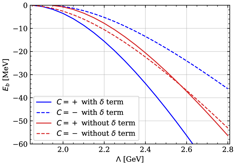
The Schrödinger equations for both $K\bar{K}_{1}(1400)$ and $K\bar{K}_{1}(1270)$ systems are solved numerically. For the isovector cases, no bound states are found since contributions from $\rho$ and $\omega$ exchanges cancel with each other. Now we focus on the isoscalar cases. The binding energies for $K\bar{K}_{1}(1400)$ with different cutoffs are shown in Fig. 2. We can see that the $1^{-+}$ system can form a bound state when $\Lambda\gtrsim 1.9$ GeV. We need $\Lambda\approx 2.5$ GeV to produce a binding energy of 40 MeV, the experimental value of the newly observed exotic state by BESIII. With the same cutoff, the binding energy of the $1^{--}$ $K\bar{K}_{1}(1400)$ state is predicted to be $10\sim 30$ MeV where the uncertainty comes from whether the $\delta$ potential is included or not. Due to the large coupling of $K_{1}(1270)KV$, the potential between $K\bar{K}_{1}(1270)$ is repulsive for $C=+$ and therefore, no bound states are expected. On the other hand, the potential is too attractive for $C=-$ to form a molecule with a reasonable binding energy if we use a cutoff about $2.5$ GeV. Even when $\Lambda\sim 1.5$ GeV the binding energy is larger than 100 MeV, which is not acceptable for a shallow bound state, for which our previous treatments hold valid.

With reasonable cutoff we have obtained the possible bound states of $K\bar{K}_{1}(1400)$ with $J^{PC}=1^{-\pm}$, denoted as $X$ temporarily. It is now desirable to estimate the decay patterns of the predicted molecular states, especially the $\eta\eta^{\prime}$ channel, to compare with BESIII observation and provide guidance to further experimental investigations. It is natural that such molecules decay through their components, as illustrated in Fig. 3. Since $K_{1}$’s have a quite large decay width, we assume that the three-body decays of the molecules are dominated by the process shown in the right diagram in Fig. 3, where $P,V=\pi,K^{*}$ or $K,\rho/\omega$. Two-body strong decay channels considered here are listed in Table 1.

The coupling between a hadronic molecule and its components can be constructed as

where $y$ is the coupling constant and $X$ denotes the field of the molecule. For a loosely bound state, one can estimate the coupling constant in a model-independent way by means of Weinberg compositeness criterion Weinberg (1965); Baru et al. (2004); Guo et al. (2018), which is developed to estimate the amount of compact and molecular components in a given state, where the molecular components consist of two stable (or narrow ²²2“narrow” is relative to the binding energy of that molecular state, that is, the widths of the molecular components should be much smaller than its binding energy.) compact states. However, $K_{1}(1400)$ has a width of 174 MeV, much larger than the obtained binding energy in our case. Strictly speaking, one should consider the dynamics between the sub-ingredients of $K_{1}(1400)$ and kaon, such as $K\bar{K}^{*}\pi$ three-body system, like what were done for $X(3872)$ Baru et al. (2011) and $T_{cc}^{+}$ Du et al. (2022). On the other hand, the decay width of $K_{1}(1400)$ is much smaller than the masses of exchanged $\rho$ and $\omega$, and hence it should not jeopardize the molecular interpretation of $\eta_{1}(1855)$ as argued in Ref. Guo and Meissner (2011).

To obtain a better estimate of the coupling $y$, we consider in the following the pole position of the $X$ on the complex $\sqrt{s}$ plane by assuming that the $X$ is a purely molecular state of $K\bar{K}_{1}(1400)$. The dominant decay channel of $K_{1}(1400)$ is $K^{*}\pi$ with a branching ratio of 94% and for simplicity, we take it to be 100% by ignoring all other channels. The pole position of $K\bar{K}(1400)$ system with coupled channel effects ignored is determined by

where $V$, assumed to be constant, is the interaction strength of $K\bar{K}(1400)$ and $G$ is the scalar two particle loop propagator,

with $P$ the total momentum. Note that we have ignored the spin structures of the intermediate $K_{1}$, the corrections from which, as argued in Refs Roca et al. (2005); Molina et al. (2008), are at the order of $l_{\rm on}^{2}/m_{K_{1}}^{2}$ with $l_{\rm on}$ the on-shell 3-momentum of $K\bar{K}_{1}$. A hard cutoff, $\Lambda$, of the 3-momentum $\bm{l}$ will be introduced to regularize the UV divergence. The running width of $K_{1}$ reads

with $g_{K_{1}}=3.65$ GeV the coupling constant of $K_{1}K^{*}\pi$ and $\bm{q}$, depending on $s$, the 3-momentum of $K^{*}$ in the center of mass frame of $K_{1}$.

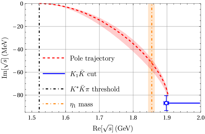
The pole trajectory when varying $V$ is shown in Fig. 4. As expected, the partial width of $\eta_{1}(1855)\to K(\bar{K}_{1}(1400)\to\bar{K}^{*}\pi)$ gets smaller when the binding energy becomes larger and the pole will touch the $K\bar{K}_{1}(1400)$ cut, around $1900-i87$ MeV, if the binding energy goes to zero. For the measured $\eta_{1}$ mass, the three body decay width of $X$ is around $105$ MeV, which weakly depends on the hard cutoff $\Lambda$ in the phenomenological reasonable range of $0.6\sim 1$ GeV. By matching the three body decay width of $X$ to the obtained pole position, we have an estimate of the coupling constant,

We refer to our previous work for other relevant couplings Dong and Zou (2021). In particular, a non-zero $D$-wave component is introduced in the vertex $K_{1}K^{*}\pi$ and $K_{1}K^{*}\eta$ as similar with $D_{1}D^{*}\pi$ interaction used in Ref. Dong and Zou (2021). The ratio of $D$-wave component over the $S$-wave from RPP Zyla et al. (2020) is $0.04\pm 0.01$. When performing the loop integral in the triangle diagram of the two-body decays, a Gaussian regulator $f_{1}$ (at the vertex of $XK\bar{K}_{1}$) and a multipole form factor $f_{2}$ (at one of the vertices where the exchanged particle $A$ is involved), formulated as follows, are included to regularize the ultraviolet divergence.

where $\bm{p}$ are the three dimensional space part of momentum of $K$ or $\bar{K}_{1}$, $m$ and $q$ is the mass and momentum of the exchanged particle.

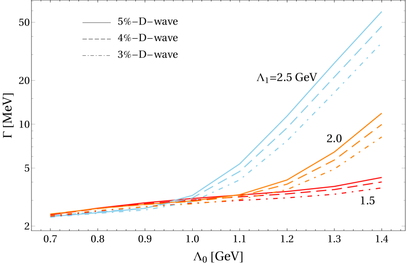
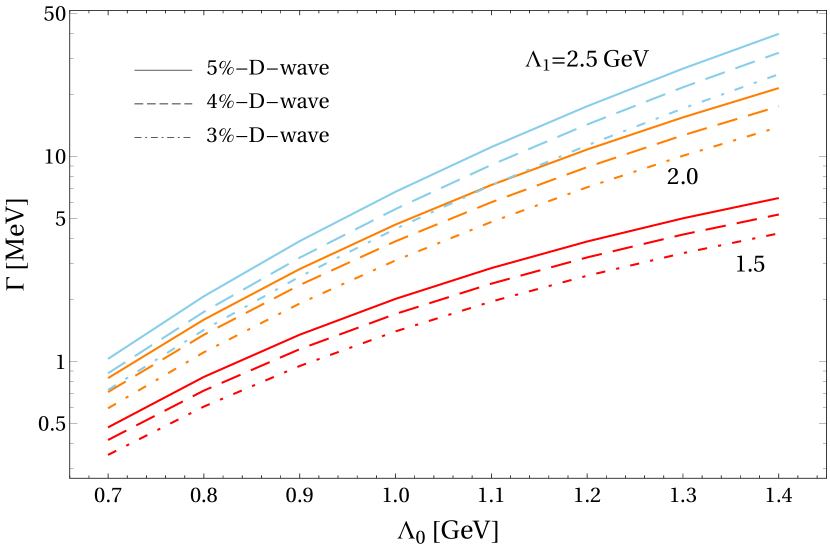
The decay patterns of $1^{--}$ and $1^{-+}$ $K\bar{K}_{1}(1400)$ molecules for $\Lambda_{0}=1.3$ GeV and $\Lambda_{1}=2.5$ GeV are shown in Table 1. Our results show that the three-body $K\bar{K}^{*}\pi$ is the largest decay channel for both $1^{--}$ and $1^{-+}$ $K\bar{K}_{1}$ molecules. And their dominant two-body decay channel is also the same, i.e., $K^{*}\bar{K}^{*}$. Moreover, the $1^{-+}$ exotic state also couples strongly to the $\eta\eta^{\prime}$ channel. It is quite similar with the properties of $D\bar{D}_{1}$ molecules where the $D^{*}\bar{D}^{*}$ and $\eta\eta_{c}$ channels contribute dominantly to the two-body decay widths Dong et al. (2020). In general, one can find that the molecular scenario always seems to support the strong couplings with the open-flavor channels. In addition, we find that the $1^{-+}$ molecule has also a strong coupling with $a_{1}\pi$ channel, which is also reflected in a recent lattice simulation Woss et al. (2021). In that work, the exotic $1^{-+}$ hybird meson with negative $G$-parity decays dominantly into $b_{1}\pi$ channel which translates to $a_{1}\pi$ channel for the positive $G$-parity $1^{-+}$ state. The parameter sensitivity of partial widths of two dominant two-body decay channels for the $1^{-+}$ $K\bar{K}_{1}(1400)$ molecule, namely $K^{*}\bar{K}^{*}$ and $\eta\eta^{\prime}$, is presented in Fig. 5.

We have used the one boson exchange potential between the $K\bar{K}_{1}$, for both $J^{PC}=1^{--}$ and $J^{PC}=1^{-+}$ systems, to investigate if it is possible for them to form bound states. It turns out that with a momentum cutoff $\Lambda\approx 2.5$ GeV, the attractive force between $K\bar{K}_{1}(1400)$ with $J^{PC}=1^{-+}$ is strong enough to form a bound state with a binding energy of around 40 MeV, which can be related to the newly observed $\eta_{1}(1855)$. The C-parity partner of this molecule is predicted to exist with a binding energy around 10 $\sim$ 30 MeV. While for the $K_{1}(1270)$, the strong coupling between $K_{1}(1270)KV$ results in a repulsive force for $C=+$ and a much deeply attractive force for $C=-$, neither of which is expected to form a molecular state.

The decay properties of the two possible molecules of $K\bar{K}_{1}(1400)$ are investigated. For both the $1^{--}$ and $1^{-+}$ states, the three body channel $K\bar{K}^{*}\pi$ dominates due to the large decay width of $K_{1}(1400)\to K^{*}\pi$. The $K^{*}\bar{K}^{*}$ and $\eta\eta^{\prime}$ channels have the largest contributions among the two body decays. The presented decay pattern of $1^{-+}$ $K\bar{K}_{1}(1400)$ molecule is compatible with BESIII’s measurements.

In summary, it is shown that the newly observed exotic state $\eta_{1}(1855)$ can be explained as a $K\bar{K}_{1}(1400)$ molecule. This interpretation can be checked by searching for $\eta_{1}(1855)$ in $\omega\phi$ channel and its $C$-partner in $\pi\rho$, $\eta\omega$ and $K\bar{K}$ channels, in addition to $K^{*}\bar{K}^{*}$ channel.

We thank Feng-Kun Guo, Xiao-Yu Li, Jia-Jun Wu and Mao-Jun Yan for useful discussions. This work is supported by the NSFC and the Deutsche Forschungsgemeinschaft (DFG, German Research Foundation) through the funds provided to the Sino German Collaborative Research Center TRR110 Symmetries and the Emergence of Structure in QCD (NSFC Grant No.12070131001, DFG Project-ID 196253076-TRR 110), by the NSFC Grants No. 11835015 and No. 12047503, and by the Chinese Academy of Sciences (CAS) under Grant No.XDB34030000.

References

- Gell-Mann (1964) M. Gell-Mann, Phys. Lett. 8, 214 (1964).
- Zweig (1964) G. Zweig, “An SU(3) model for strong interaction symmetry and its breaking. Version 2,” in DEVELOPMENTS IN THE QUARK THEORY OF HADRONS. VOL. 1. 1964 - 1978, edited by D. B. Lichtenberg and S. P. Rosen (1964) pp. 22–101.
- Klempt and Zaitsev (2007) E. Klempt and A. Zaitsev, Phys. Rept. 454, 1 (2007), arXiv:0708.4016 [hep-ph] .
- Dalitz and Tuan (1959) R. H. Dalitz and S. F. Tuan, Phys. Rev. Lett. 2, 425 (1959).
- Dalitz and Tuan (1960) R. H. Dalitz and S. F. Tuan, Annals Phys. 10, 307 (1960).
- Alston et al. (1961) M. H. Alston, L. W. Alvarez, P. Eberhard, M. L. Good, W. Graziano, H. K. Ticho, and S. G. Wojcicki, Phys. Rev. Lett. 6, 698 (1961).
- Hyodo and Niiyama (2021) T. Hyodo and M. Niiyama, Prog. Part. Nucl. Phys. 120, 103868 (2021), arXiv:2010.07592 [hep-ph] .
- Mai (2021) M. Mai, Eur. Phys. J. ST 230, 1593 (2021), arXiv:2010.00056 [nucl-th] .
- Choi et al. (2003) S. K. Choi et al. (Belle), Phys. Rev. Lett. 91, 262001 (2003), arXiv:hep-ex/0309032 .
- Chen et al. (2016) H.-X. Chen, W. Chen, X. Liu, and S.-L. Zhu, Phys. Rept. 639, 1 (2016), arXiv:1601.02092 [hep-ph] .
- Hosaka et al. (2016) A. Hosaka, T. Iijima, K. Miyabayashi, Y. Sakai, and S. Yasui, PTEP 2016, 062C01 (2016), arXiv:1603.09229 [hep-ph] .
- Richard (2016) J.-M. Richard, Few Body Syst. 57, 1185 (2016), arXiv:1606.08593 [hep-ph] .
- Lebed et al. (2017) R. F. Lebed, R. E. Mitchell, and E. S. Swanson, Prog. Part. Nucl. Phys. 93, 143 (2017), arXiv:1610.04528 [hep-ph] .
- Esposito et al. (2017) A. Esposito, A. Pilloni, and A. D. Polosa, Phys. Rept. 668, 1 (2017), arXiv:1611.07920 [hep-ph] .
- Guo et al. (2018) F.-K. Guo, C. Hanhart, U.-G. Meißner, Q. Wang, Q. Zhao, and B.-S. Zou, Rev. Mod. Phys. 90, 015004 (2018), arXiv:1705.00141 [hep-ph] .
- Ali et al. (2017) A. Ali, J. S. Lange, and S. Stone, Prog. Part. Nucl. Phys. 97, 123 (2017), arXiv:1706.00610 [hep-ph] .
- Olsen et al. (2018) S. L. Olsen, T. Skwarnicki, and D. Zieminska, Rev. Mod. Phys. 90, 015003 (2018), arXiv:1708.04012 [hep-ph] .
- Altmannshofer et al. (2019) W. Altmannshofer et al. (Belle-II), PTEP 2019, 123C01 (2019), [Erratum: PTEP 2020, 029201 (2020)], arXiv:1808.10567 [hep-ex] .
- Kalashnikova and Nefediev (2019) Y. S. Kalashnikova and A. V. Nefediev, Phys. Usp. 62, 568 (2019), arXiv:1811.01324 [hep-ph] .
- Cerri et al. (2019) A. Cerri et al., CERN Yellow Rep. Monogr. 7, 867 (2019), arXiv:1812.07638 [hep-ph] .
- Liu et al. (2019) Y.-R. Liu, H.-X. Chen, W. Chen, X. Liu, and S.-L. Zhu, Prog. Part. Nucl. Phys. 107, 237 (2019), arXiv:1903.11976 [hep-ph] .
- Brambilla et al. (2020) N. Brambilla, S. Eidelman, C. Hanhart, A. Nefediev, C.-P. Shen, C. E. Thomas, A. Vairo, and C.-Z. Yuan, Phys. Rept. 873, 1 (2020), arXiv:1907.07583 [hep-ex] .
- Guo et al. (2020) F.-K. Guo, X.-H. Liu, and S. Sakai, Prog. Part. Nucl. Phys. 112, 103757 (2020), arXiv:1912.07030 [hep-ph] .
- Yang et al. (2020) G. Yang, J. Ping, and J. Segovia, Symmetry 12, 1869 (2020), arXiv:2009.00238 [hep-ph] .
- Ortega and Entem (2021) P. G. Ortega and D. R. Entem, Symmetry 13, 279 (2021), arXiv:2012.10105 [hep-ph] .
- Dong et al. (2021a) X.-K. Dong, F.-K. Guo, and B.-S. Zou, Progr. Phys. 41, 65 (2021a), arXiv:2101.01021 [hep-ph] .
- Dong et al. (2021b) X.-K. Dong, F.-K. Guo, and B.-S. Zou, Commun. Theor. Phys. 73, 125201 (2021b), arXiv:2108.02673 [hep-ph] .
- Godfrey and Isgur (1985) S. Godfrey and N. Isgur, Phys. Rev. D 32, 189 (1985).
- Capstick and Isgur (1985) S. Capstick and N. Isgur, AIP Conf. Proc. 132, 267 (1985).
- Aubert et al. (2005) B. Aubert et al. (BaBar), Phys. Rev. Lett. 95, 142001 (2005), arXiv:hep-ex/0506081 .
- Ablikim et al. (2013) M. Ablikim et al. (BESIII), Phys. Rev. Lett. 110, 252001 (2013), arXiv:1303.5949 [hep-ex] .
- Liu et al. (2013) Z. Q. Liu et al. (Belle), Phys. Rev. Lett. 110, 252002 (2013), [Erratum: Phys.Rev.Lett. 111, 019901 (2013)], arXiv:1304.0121 [hep-ex] .
- Ablikim et al. (2021) M. Ablikim et al. (BESIII), Phys. Rev. Lett. 126, 102001 (2021), arXiv:2011.07855 [hep-ex] .
- Aaij et al. (2015) R. Aaij et al. (LHCb), Phys. Rev. Lett. 115, 072001 (2015), arXiv:1507.03414 [hep-ex] .
- Aaij et al. (2019) R. Aaij et al. (LHCb), Phys. Rev. Lett. 122, 222001 (2019), arXiv:1904.03947 [hep-ex] .
- Aaij et al. (2021a) R. Aaij et al. (LHCb), Sci. Bull. 66, 1391 (2021a), arXiv:2012.10380 [hep-ex] .
- Aaij et al. (2021b) R. Aaij et al. (LHCb), (2021b), arXiv:2109.01038 [hep-ex] .
- Aaij et al. (2021c) R. Aaij et al. (LHCb), (2021c), arXiv:2109.01056 [hep-ex] .
- Zyla et al. (2020) P. A. Zyla et al. (Particle Data Group), PTEP 2020, 083C01 (2020).
- Kuhn et al. (2004) J. Kuhn et al. (E852), Phys. Lett. B 595, 109 (2004), arXiv:hep-ex/0401004 .
- Lu et al. (2005) M. Lu et al. (E852), Phys. Rev. Lett. 94, 032002 (2005), arXiv:hep-ex/0405044 .
- Meyer and Swanson (2015) C. A. Meyer and E. S. Swanson, Prog. Part. Nucl. Phys. 82, 21 (2015), arXiv:1502.07276 [hep-ph] .
- Ablikim et al. (2022a) M. Ablikim et al. (BESIII), (2022a), arXiv:2202.00621 [hep-ex] .
- Ablikim et al. (2022b) M. Ablikim et al. (BESIII), (2022b), arXiv:2202.00623 [hep-ex] .
- Chen et al. (2022) H.-X. Chen, N. Su, and S.-L. Zhu, (2022), arXiv:2202.04918 [hep-ph] .
- Qiu and Zhao (2022) L. Qiu and Q. Zhao, (2022), arXiv:2202.00904 [hep-ph] .
- Burakovsky and Goldman (1997) L. Burakovsky and J. T. Goldman, Phys. Rev. D 56, R1368 (1997), arXiv:hep-ph/9703274 .
- Suzuki (1993) M. Suzuki, Phys. Rev. D 47, 1252 (1993).
- Cheng (2003) H.-Y. Cheng, Phys. Rev. D 67, 094007 (2003), arXiv:hep-ph/0301198 .
- Yang (2011) K.-C. Yang, Phys. Rev. D 84, 034035 (2011), arXiv:1011.6113 [hep-ph] .
- Hatanaka and Yang (2008) H. Hatanaka and K.-C. Yang, Phys. Rev. D 77, 094023 (2008), [Erratum: Phys.Rev.D 78, 059902 (2008)], arXiv:0804.3198 [hep-ph] .
- Tayduganov et al. (2012) A. Tayduganov, E. Kou, and A. Le Yaouanc, Phys. Rev. D 85, 074011 (2012), arXiv:1111.6307 [hep-ph] .
- Divotgey et al. (2013) F. Divotgey, L. Olbrich, and F. Giacosa, Eur. Phys. J. A 49, 135 (2013), arXiv:1306.1193 [hep-ph] .
- Zhang et al. (2018) Z.-Q. Zhang, H. Guo, and S.-Y. Wang, Eur. Phys. J. C 78, 219 (2018), arXiv:1705.00524 [hep-ph] .
- Roca et al. (2005) L. Roca, E. Oset, and J. Singh, Phys. Rev. D 72, 014002 (2005), arXiv:hep-ph/0503273 .
- Geng et al. (2007) L. S. Geng, E. Oset, L. Roca, and J. A. Oller, Phys. Rev. D 75, 014017 (2007), arXiv:hep-ph/0610217 .
- Wang et al. (2019) G. Y. Wang, L. Roca, and E. Oset, Phys. Rev. D 100, 074018 (2019), arXiv:1907.09188 [hep-ph] .
- Meissner (1988) U. G. Meissner, Phys. Rept. 161, 213 (1988).
- Zhang et al. (2006) Y.-J. Zhang, H.-C. Chiang, P.-N. Shen, and B.-S. Zou, Phys. Rev. D 74, 014013 (2006), arXiv:hep-ph/0604271 .
- Dong and Zou (2021) X.-K. Dong and B.-S. Zou, Eur. Phys. J. A 57, 139 (2021), arXiv:2009.11619 [hep-ph] .
- Dong et al. (2020) X.-K. Dong, Y.-H. Lin, and B.-S. Zou, Phys. Rev. D 101, 076003 (2020), arXiv:1910.14455 [hep-ph] .
- Casalbuoni et al. (1997) R. Casalbuoni, A. Deandrea, N. Di Bartolomeo, R. Gatto, F. Feruglio, and G. Nardulli, Phys. Rept. 281, 145 (1997), arXiv:hep-ph/9605342 .
- Isola et al. (2003) C. Isola, M. Ladisa, G. Nardulli, and P. Santorelli, Phys. Rev. D 68, 114001 (2003), arXiv:hep-ph/0307367 .
- Bardeen et al. (2003) W. A. Bardeen, E. J. Eichten, and C. T. Hill, Phys. Rev. D 68, 054024 (2003), arXiv:hep-ph/0305049 .
- Tornqvist (1994) N. A. Tornqvist, Z. Phys. C 61, 525 (1994), arXiv:hep-ph/9310247 .
- Burns and Swanson (2019) T. J. Burns and E. S. Swanson, Phys. Rev. D 100, 114033 (2019), arXiv:1908.03528 [hep-ph] .
- Yalikun et al. (2021) N. Yalikun, Y.-H. Lin, F.-K. Guo, Y. Kamiya, and B.-S. Zou, Phys. Rev. D 104, 094039 (2021), arXiv:2109.03504 [hep-ph] .
- Weinberg (1965) S. Weinberg, Phys. Rev. 137, B672 (1965).
- Baru et al. (2004) V. Baru, J. Haidenbauer, C. Hanhart, Y. Kalashnikova, and A. E. Kudryavtsev, Phys. Lett. B 586, 53 (2004), arXiv:hep-ph/0308129 .
- Baru et al. (2011) V. Baru, A. A. Filin, C. Hanhart, Y. S. Kalashnikova, A. E. Kudryavtsev, and A. V. Nefediev, Phys. Rev. D 84, 074029 (2011), arXiv:1108.5644 [hep-ph] .
- Du et al. (2022) M.-L. Du, V. Baru, X.-K. Dong, A. Filin, F.-K. Guo, C. Hanhart, A. Nefediev, J. Nieves, and Q. Wang, Phys. Rev. D 105, 014024 (2022), arXiv:2110.13765 [hep-ph] .
- Guo and Meissner (2011) F.-K. Guo and U.-G. Meissner, Phys. Rev. D 84, 014013 (2011), arXiv:1102.3536 [hep-ph] .
- Molina et al. (2008) R. Molina, D. Nicmorus, and E. Oset, Phys. Rev. D 78, 114018 (2008), arXiv:0809.2233 [hep-ph] .
- Woss et al. (2021) A. J. Woss, J. J. Dudek, R. G. Edwards, C. E. Thomas, and D. J. Wilson (Hadron Spectrum), Phys. Rev. D 103, 054502 (2021), arXiv:2009.10034 [hep-lat] .