Interval Estimation of the Unknown Exponential Parameter Based on Time Truncated Data
Abstract
In this paper we consider the statistical inference of the unknown parameter of an exponential distribution based on the time truncated data. The time truncated data occurs quite often in the reliability analysis for type-I or hybrid censoring cases. All the results available today are based on the conditional argument that at least one failure occurs during the experiment. In this paper we provide some inferential results based on the unconditional argument. We extend the results for some two-parameter distributions also.
Key Words and Phrases: Exponential distribution; type-I censoring; hybrid censoring; conjugate prior; confidence interval; credible interval.
AMS Subject Classifications: 62F10, 62F03, 62H12.
1 Department of Mathematics and Statistics, Indian Institute of Technology Kanpur, Pin 208016, India. E-mail: arnab@iitk.ac.in.
2 Department of Mathematics and Statistics, Indian Institute of Technology Kanpur, Pin 208016, India. Corresponding author, E-mail: kundu@iitk.ac.in, Phone no. 91-512-2597141, Fax no. 91-512-2597500.
1 Introduction
Let be a random sample from an exponential distribution with parameter , then it has the following probability density function (PDF)
| (1) |
Here is the natural parameter space. Since for = 0, as defined in (1) is not a proper PDF, we are not including the point 0 in the parameter space. Suppose items are tested and their ordered failure times are denoted by . If the experiment is stopped at a prefixed time then it results in a simple type-I censoring case. Let there be failures in . Then and , although are not observed. Here is a random variable that can take the values . The main aim of this note is to draw inference on , based on observations.
This is an old problem and Bartholomew (1963) was the first to consider it. He considered the following form of the exponential PDF;
| (2) |
He considered as the parameter space of . In this case the maximum likelihood estimator (MLE) of does not exist when . Hence all the inferences related to are based on the conditional argument that . Later on a series of papers starting with Chen and Bhattacharyya (1988) and then continuing with Gupta and Kundu (1998) and Childs et al. (2003) considered type-I hybrid censoring case for the model (2), and obtained the exact inference on based on the conditional argument that .
In case of type-I censoring, and this probability can be quite high for small value of . The natural question here is whether it is possible to draw any inference on , when . The second aim of the study is to determine if there exists any significant difference between the conditional and unconditional inference. For example, in this paper it has been shown that it is possible to construct an exact 100 confidence interval of even when = 0. Following the approach of Chen and Bhattacharyya (1998), an exact 100 confidence interval of also can be obtained based on the conditional MLE of , conditioning on the event that . The question is whether the lengths of the confidence intervals based on the two different approaches are significantly different or not. We perform some simulation experiments to compare the confidence intervals based on the two different methods. We further obtain the Bayes estimate and the associated credible interval of the unknown parameter based on the non-informative prior. Finally the results are extended for the two-parameter exponential, Weibull and generalized exponential distributions also.
Rest of the paper is organized as follows. In Section 2, we provide two different constructions of confidence intervals and the Bayesian credible intervals. The simulation results for confidence and credible intervals of the parameter are provided in Section 3. In Section 4, we extend the results for the two parameter exponential, Weibull and generalized exponential distributions, and finally we conclude the paper in Section 5.
2 Construction of Confidence and Credible Intervals
In this section we proceed to construct the confidence and credible intervals of the parameter of interest , based on a new estimator of and the posterior distribution of , respectively.
2.1 Confidence interval (CI)
Based on the observations from the model (1), the likelihood function becomes
| (3) |
Note that the MLE of does not exist when . It exists only if and it is given by
Now based on , the joint sufficient statistic for , we define a new estimator of for all as follows
| (4) |
Note that, is equal to only when . Now we provide the exact distribution of , which will be useful in constructing an exact confidence interval of .
Theorem 1
The distribution of for , can be written as,
| (5) |
where
and , is the incomplete gamma function.
Proof: For , can be written as,
| (6) | |||||
Note that the expression of can be obtained by using the moment generating function approach. Refer to Corollary 2.2 of Childs et al. (2003) or equation (8) of Gupta and Kundu (1998) for it. It is possible to obtain (5) in terms of the chi-square integral as in Bartholomew (1963). The distribution of is a mixture of discrete and continuous distributions. The following corollary comes from Theorem 1.
Corollary 1
and for , the PDF of is given by
| (7) |
where
| (8) |
Now we consider the construction of an exact 100 confidence interval of . We need the following lemma for further development.
Lemma 1
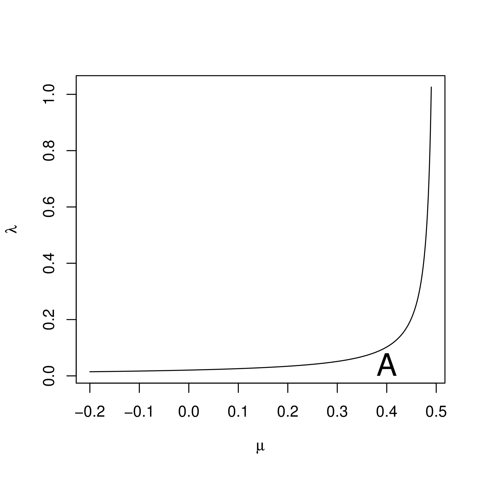
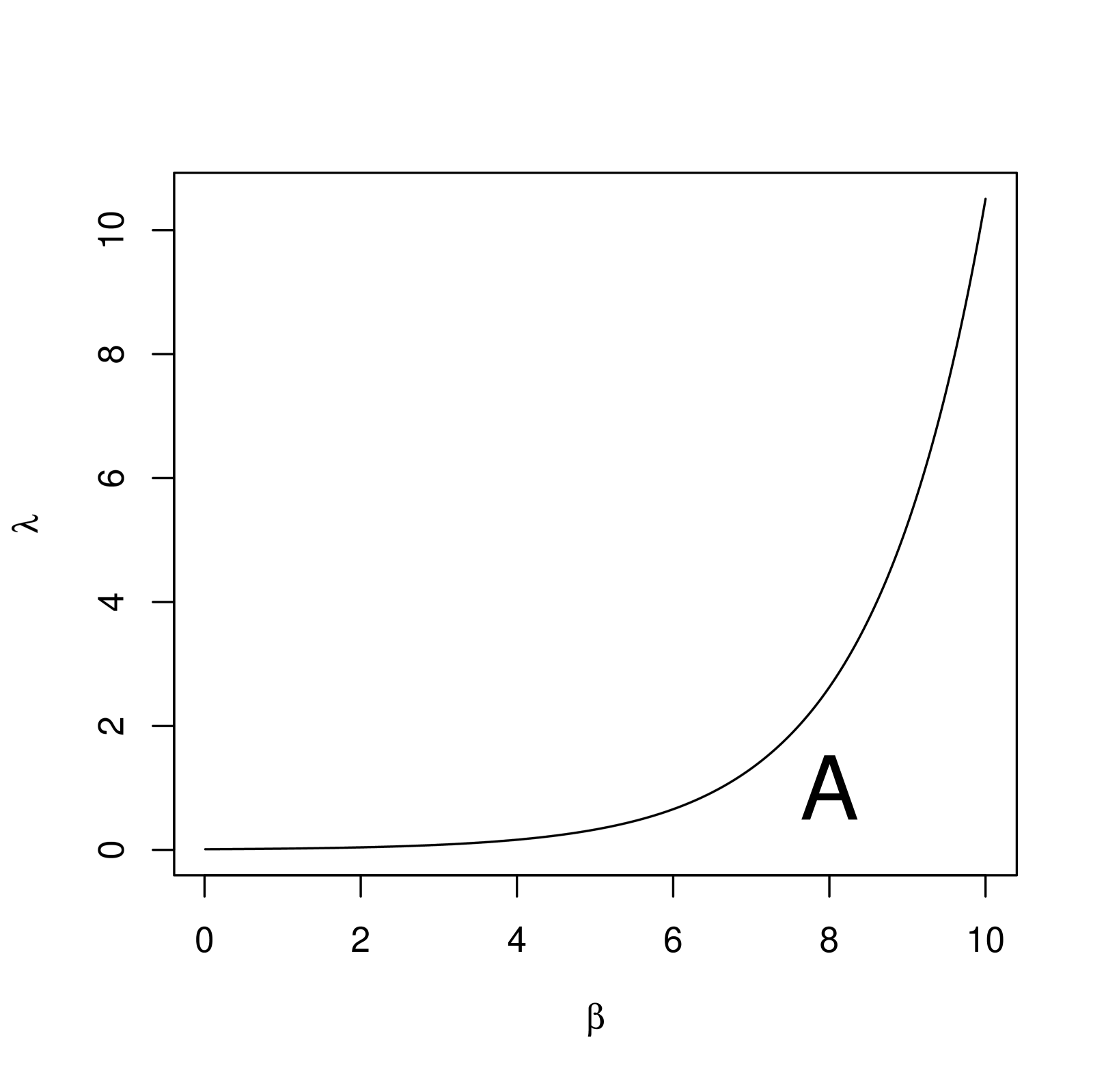
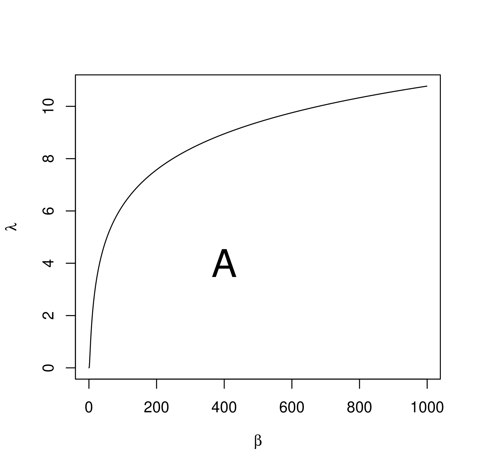
For a fixed , is a monotonically decreasing function of .
Proof: The proof can be obtained along the same line as the proof of the three monotonic lemmas by Balakrishnan and Iliopoulos (2009).
A graphical plot (Figure 1) of as a function of for a fixed value of is provided for a visual illustration. Here we have taken = 5, = 0.5 and = 1.

We now provide an exact 100 confidence interval of for different values of .
Case-I: Construction of CI when :
Since and it is a decreasing function of , a one sided 100 confidence interval of can be obtained as .
Hence,
Case-II: Construction of CI when :
A symmetric
100 confidence interval, , of can be obtained by solving the following two non-linear equations
| (9) |
These non-linear equations are to be solved using standard non-linear solver viz. Newton Rapshon, bisection method etc.
2.2 Credible interval (CRI)
In this subsection we will discuss constructing a 100 credible interval of based on the conjugate prior on . It is assumed that has a natural gamma prior with the shape and scale parameters as and , respectively with the following PDF
| (10) |
Therefore the posterior density function of becomes
| (11) |
Hence the Bayes estimate of under the squared error loss function becomes
| (12) |
The associated 100 symmetric credible interval of can be obtained as , where and can be obtained as the solutions of
| (13) |
respectively. Here is the incomplete gamma function and . Observe that, when , the Bayes estimate of matches with , although it is an improper prior. Therefore, the comparison of the confidence intervals based on (9) and the credible interval based on (13) makes sense, although their interpretations are different. When = 0, the posterior density function of becomes improper for = 0. Due to this reason we propose to use a proper prior with 0 as suggested by Congdon (2014).
3 Numerical Comparisons
In this section we present some simulation results to compare the performances of the two confidence intervals and the corresponding credible intervals. We compare the performances in terms of the average lengths and the coverage percentages. Different values of , and are taken. We consider = 5, 10, 15, 20, = 0.5, 1.0, 2.0 and = 1, 2. For Bayesian inference we have taken = 0.001. All the results are based on 5,000 replications. The results are reported in Tables 1 to 3.
The following points have been revealed from these simulation experiments. In all these cases it is observed that biases and mean squared errors (MSEs) decrease as sample size increases, increases or increases as expected. Now comparing the confidence intervals and credible intervals in Tables 1 to 3 it is clear that for small sample sizes, small and small values, the confidence intervals based on unconditional distribution performs better that the credible intervals based on non-informative priors in terms of the coverage percentages. The coverage percentages of the confidence intervals based on unconditional distribution are very close to the nominal value (95%) in all cases. Although, as expected for large sample sizes they are almost equal. The confidence intervals based on the conditional distribution do not perform very well when the sample size is very small and is also small, although when the sample size is not very small it performs well. Performances of the two confidence intervals match as expected when sample size is large.
4 Some Related Models
In this section we consider some of the related two-parameter models, and construct an exact 100 confidence set of the two parameters, when items are tested and there is no observed failure during .
Model 1: A two-parameter exponential distribution with the location parameter and scale parameter having the following PDF
| (14) |
Here and . In this case . Hence, a 100 confidence set of can be obtained as . Therefore,
Model 2: Let us consider now a two-parameter Weibull distribution with the shape parameter and scale parameter which has the following PDF
| (15) |
Here and . In this case . A 100 confidence set of , can be obtained as . Hence,
Model 3: Similarly, if we consider two-parameter generalized exponential distribution which has the following PDF
| (16) |
Here is the shape parameter and is the scale parameter. Here, . A 100 confidence set of , can be obtained as . Therefore,
Joint Confidence Set
Just for illustrative purposes, taking = 5 and = 0.5, we provide the joint 100 confidence set as the shaded region of (i) for two-parameter exponential distribution, (ii) for two-parameter Weibull distribution and (iii) for two-parameter generalized exponential distribution, in Figure 2 when = 0.
5 Conclusions
In this paper we have considered the time truncated exponential distribution and provide the exact confidence interval of the unknown scale parameter based on the unconditional argument. All the existing results are based on the conditional argument and it does not provide any statistical inference of the unknown parameter when there is no observation. In this paper we have provided the inference on the scale parameter even when there is no observation. Simulation experiments are performed and it is observed that the proposed method works quite well even when the sample size is very small. The joint confidence sets have been provided for two-parameter exponential, Weibull and generalized exponential distributions also for time truncated case when there is no observation during the time period of the experiment. The results can be extended to the competing risks model also, as considered in Kundu, Kannan and Balakrishnan (2004).
| T=1 | T=2 | ||||||||
|---|---|---|---|---|---|---|---|---|---|
| Bias | MSE | CI | CP | Bias | MSE | CI | CP | ||
| 5 | 0.074 | 0.207 | 1.577 | 97.36 | 0.091 | 0.166 | 1.253 | 94.42 | |
| 10 | 0.033 | 0.080 | 1.041 | 94.10 | 0.038 | 0.055 | 0.825 | 94.62 | |
| =0.5 | 15 | 0.020 | 0.049 | 0.833 | 94.86 | 0.023 | 0.033 | 0.659 | 94.58 |
| 20 | 0.015 | 0.035 | 0.716 | 94.86 | 0.016 | 0.023 | 0.565 | 94.96 | |
| 5 | 0.182 | 0.662 | 2.505 | 94.42 | 0.226 | 0.619 | 2.240 | 94.50 | |
| 10 | 0.076 | 0.221 | 1.649 | 94.62 | 0.092 | 0.181 | 1.434 | 94.60 | |
| =1.0 | 15 | 0.046 | 0.132 | 1.318 | 94.58 | 0.056 | 0.104 | 1.139 | 94.56 |
| 20 | 0.032 | 0.092 | 1.130 | 94.98 | 0.040 | 0.071 | 0.974 | 94.86 | |
| 5 | 0.452 | 2.477 | 4.481 | 94.50 | 0.510 | 2.428 | 4.351 | 94.66 | |
| 10 | 0.183 | 0.724 | 2.869 | 94.60 | 0.214 | 0.688 | 2.742 | 94.42 | |
| =2.0 | 15 | 0.112 | 0.416 | 2.278 | 94.56 | 0.131 | 0.390 | 2.162 | 94.92 |
| 20 | 0.081 | 0.284 | 1.948 | 94.86 | 0.094 | 0.260 | 1.843 | 94.92 |
| T=1 | T=2 | ||||||||
|---|---|---|---|---|---|---|---|---|---|
| Bias | MSE | CI | CP | Bias | MSE | CI | CP | ||
| 5 | 0.067 | 0.185 | 1.398 | 69.28 | 0.088 | 0.156 | 1.241 | 91.28 | |
| 10 | 0.034 | 0.072 | 1.037 | 92.74 | 0.038 | 0.055 | 0.826 | 94.62 | |
| =0.5 | 15 | 0.021 | 0.048 | 0.837 | 94.96 | 0.023 | 0.033 | 0.659 | 94.58 |
| 20 | 0.016 | 0.035 | 0.718 | 94.88 | 0.016 | 0.023 | 0.565 | 94.96 | |
| 5 | 0.176 | 0.623 | 2.482 | 91.28 | 0.226 | 0.618 | 2.245 | 94.48 | |
| 10 | 0.076 | 0.219 | 1.652 | 94.62 | 0.092 | 0.181 | 1.435 | 94.60 | |
| =1.0 | 15 | 0.046 | 0.132 | 1.318 | 94.58 | 0.056 | 0.104 | 1.139 | 94.56 |
| 20 | 0.032 | 0.092 | 1.130 | 94.98 | 0.040 | 0.071 | 0.974 | 94.86 | |
| 5 | 0.452 | 2.471 | 4.490 | 94.48 | 0.510 | 2.428 | 4.352 | 94.66 | |
| 10 | 0.184 | 0.724 | 2.869 | 94.60 | 0.214 | 0.688 | 2.742 | 94.42 | |
| =2.0 | 15 | 0.112 | 0.416 | 2.278 | 94.56 | 0.131 | 0.390 | 2.162 | 94.92 |
| 20 | 0.081 | 0.284 | 1.948 | 94.86 | 0.094 | 0.260 | 1.843 | 94.92 |
| T=1 | T=2 | ||||||||
|---|---|---|---|---|---|---|---|---|---|
| Bias | MSE | CRI | CP | Bias | MSE | CRI | CP | ||
| 5 | 0.074 | 0.207 | 1.390 | 89.36 | 0.091 | 0.166 | 1.202 | 90.42 | |
| 10 | 0.033 | 0.080 | 0.985 | 92.36 | 0.038 | 0.055 | 0.807 | 93.78 | |
| =0.5 | 15 | 0.020 | 0.049 | 0.804 | 94.94 | 0.023 | 0.033 | 0.649 | 93.76 |
| 20 | 0.015 | 0.035 | 0.697 | 93.28 | 0.016 | 0.023 | 0.559 | 94.28 | |
| 5 | 0.182 | 0.662 | 2.404 | 90.42 | 0.226 | 0.619 | 2.212 | 93.54 | |
| 10 | 0.076 | 0.221 | 1.614 | 93.78 | 0.092 | 0.181 | 1.424 | 94.04 | |
| =1.0 | 15 | 0.046 | 0.132 | 1.299 | 93.76 | 0.056 | 0.104 | 1.134 | 94.04 |
| 20 | 0.032 | 0.092 | 1.117 | 94.28 | 0.040 | 0.071 | 0.970 | 94.58 | |
| 5 | 0.452 | 2.477 | 4.422 | 93.54 | 0.510 | 2.428 | 4.343 | 94.46 | |
| 10 | 0.183 | 0.724 | 2.849 | 94.04 | 0.214 | 0.688 | 2.738 | 94.26 | |
| =2.0 | 15 | 0.112 | 0.416 | 2.267 | 94.06 | 0.131 | 0.390 | 2.161 | 94.76 |
| 20 | 0.081 | 0.284 | 1.941 | 94.58 | 0.094 | 0.260 | 1.842 | 94.80 |
References
- [1] Bartholomew, D.J. (1963), ”The sampling distribution of an estimate arising in life testing”, Technometrics, vol. 5, 361-372.
- [2] Balakrishnan, N. and Iliopoulos, G. (2009), “Stochastic monotonicity of the MLE of exponential mean under different censoring scheme”, Annals of the Institute of Statistical Mathematics, vol. 61, 753 - 772.
- [3] Chen, S.M., Bhattayacharya, G.K. (1998), ”Exact confidence bound for an exponential parameter under hybrid censoring”, Communication in Statistics Theory and Methodology, 2429-2442.
- [4] Childs, A., Chandrasekhar, B., Balakrishnan, N. and Kundu, D. (2003), “Exact likelihood inference based on type-I and type-II hybrid censored samples from the exponential distribution”, Annals of the Institute of Statistical Mathematics, vol. 55, 319 - 330.
- [5] Congdon, P. (2014), Applied Bayesian Modelling, 2nd edition, Wiley, New York.
- [6] Gupta, R.D. and Kundu, D. (1998), “Hybrid censoring schemes with exponential failure distribution”, Communications in Statistics - Theory and Methods, vol. 27, 3065 - 3083.
- [7] Kundu, D., Kannan, N. and Balakrishnan, N. (2004), “Analysis of progressively censored competing risks data”, Handbook of Statistics, vol. 23, Eds. N. Balakrishnan and C.R. Rao, 331 - 348.