Intrinsic Dimension Estimation Using Wasserstein Distances
Abstract
It has long been thought that high-dimensional data encountered in many practical machine learning tasks have low-dimensional structure, i.e., the manifold hypothesis holds. A natural question, thus, is to estimate the intrinsic dimension of a given population distribution from a finite sample. We introduce a new estimator of the intrinsic dimension and provide finite sample, non-asymptotic guarantees. We then apply our techniques to get new sample complexity bounds for Generative Adversarial Networks (GANs) depending only on the intrinsic dimension of the data.
1 Introduction
Recently, practical applications of machine learning involve a very large number of features, often many more than there are samples on which to train a model. Despite this imbalance, many modern machine learning models work astonishingly well. One of the more compelling explanations for this behavior is the manifold hypothesis, which posits that, though the data appear to the practitioner in a high-dimensional, ambient space, , they really lie on (or close to) a low dimensional space of “dimension” , where we define dimension formally below. A good example to keep in mind is that of image data: each of thousands of pixels corresponds to three dimensions, but we expect that real images have some inherent structure that limits the true number of degrees of freedom in a realistic picture. This phenomenon has been thoroughly explored over the years, beginning with the linear case and moving into the more general, nonlinear regime, with such works as Niyogi et al., (2008, 2011); Belkin & Niyogi, (2001); Bickel et al., (2007); Levina & Bickel, (2004); Kpotufe, (2011); Kpotufe & Dasgupta, (2012); Kpotufe & Garg, (2013); Weed et al., (2019); Tenenbaum et al., (2000); Bernstein et al., (2000); Kim et al., (2019); Farahmand et al., (2007), among many, many others. Some authors have focused on finding representations for these lower dimensional sets (Niyogi et al.,, 2008; Belkin & Niyogi,, 2001; Tenenbaum et al.,, 2000; Roweis & Saul,, 2000; Donoho & Grimes,, 2003), while other works have focused on leveraging the low dimensionality into statistically efficient estimators (Bickel et al.,, 2007; Kpotufe,, 2011; Nakada & Imaizumi,, 2020; Kpotufe & Dasgupta,, 2012; Kpotufe & Garg,, 2013; Ashlagi et al.,, 2021).
In this work, our primary focus is on estimating the intrinsic dimension. To see why this is an important question, note that the local estimators of Bickel et al., (2007); Kpotufe, (2011); Kpotufe & Garg, (2013) and the neural network architecture of Nakada & Imaizumi, (2020) all depend in some way on the intrinsic dimension. As noted in Levina & Bickel, (2004), while a practitioner may simply apply cross-validation to select the optimal hyperparameters, this can be very costly unless the hyperparameters have a restricted range; thus, an estimate of intrinsic dimension is critical in actually applying the above works. In addition, for manifold learning, where the goal is to construct a representation of the data manifold in a lower dimensional space, the intrinsic dimension is a key parameter in many of the most popular methods (Tenenbaum et al.,, 2000; Belkin & Niyogi,, 2001; Donoho & Grimes,, 2003; Roweis & Saul,, 2000).
We propose a new estimator, based on distances between probability distributions, as well as provide rigorous, finite sample guarantees for the quality of the novel procedure. Recall that if are two measures on a metric space , then the Wasserstein- distance between and is
| (1) |
where is the set of all couplings of the two measures. If , then there are two natural metrics to put on : one is simply the restriction of the Euclidean metric to while the other is the geodesic metric in , i.e., the minimal length of a curve in that joins the points under consideration. In the sequel, if the metric is simply the Euclidean metric, we leave the Wasserstein distance unadorned to distinguish it from the intrinsic metric. For a thorough treatment of such distances, see Villani, (2008). We recall that the Hölder integral probability metric (Hölder IPM) is given by
where is the Hölder ball defined in the sequel. When , the classical result of Kantorovich-Rubinstein says that the Wasserstein and Hölder distances agree. It has been known at least since Dudley, (1969) that if a space has dimension , is a measure with support , and is the empirical measure of independent samples drawn from , then . More recently, Weed et al., (2019) has determined sharp rates for the convergence of this quantity for higher order Wasserstein distances in terms of the intrinsic dimension of the distribution. Below, we find sharp rates for the convergence of the empirical measure to the population measure with respect to the Hölder IPM: if , then and if then . These sharp rates are intuitive in that convergence to the population measure should only depend on the intrinsic complexity (i.e. dimension) without reference to the possibly much larger ambient dimension.
The above convergence results are nice theoretical insights, but they have practical value, too. The results of Dudley, (1969); Weed et al., (2019), as well as our results on the rate of convergence of the Hölder IPM, present a natural way to estimate the intrinsic dimension: take two independent samples, from and consider the ratio of or ; as , the first ratio should be about , while the second should be about , and so can be computed by taking the logarithm with respect to . The first problem with this idea is that we do not know ; to address this, we instead compute the ratios using two independent samples. A more serious issue regards how large must be in order for the asymptotic regime to apply. As we shall see below, the answer depends on the geometry of the supporting manifold.
We define two estimators: one using the intrinsic distance and the other using Euclidean distance
| (2) |
where the primes indicate independent samples of the same size and is a graph-based metric that approximates the intrinsic metric. Before we go into the details, we give an informal statement of our main theorem, which provides finite sample, non-asymptotic guarantees on the quality of the estimator111Explicit constants are given in the formal statement of Theorem 22:
Theorem 1 (Informal version of Theorem 22).
Let be a measure on supported on a compact manifold of dimension . Let be the reach of , an intrinsic geometric quantity defined below. Suppose we have independent samples from where
where is the volume of a -dimensional Euclidean unit ball. Then with probability at least , the estimated dimension satisfies
The same conclusion holds for .
Although the guarantees for and are similar, empirically is much better, as explained below. Note that the ambient dimension never enters the statistical complexity given above. While the exponential dependence on the intrinsic dimension is unfortunate, it is likely necessary as described below.
While the reach, , determines the sample complexity of our dimension estimator, consideration of the injectivity radius, , is relevant for practical application. Both geometric quantities are defined formally in the following section, but, to understand the intuition, note that, as discussed above, there are two natural metrics we could be placing on , the Euclidean metric and the geodesic distance. The reach is, intuitively, the size of the largest ball with respect to the ambient metric such that we can treat points in as if they were simply in Euclidean space; the injectivity radius is similar, except it treats neighborhoods with respect to the intrinsic metric. Considering that manifold distances are always at least as large as Euclidean distances, it is unsurprising that . Getting back to dimension estimation, specializing to the case of , and recalling (2), there are now two choices for our dimension estimator: we could use Wasserstein distance with respect to the Euclidean metric or Wasserstein distance with respect to the intrinsic metric (which we will denote by ). We will see that if , then the two estimators induced by each of these distances behave similarly, but when , the latter is better. While we wish to use to estimate the dimension, we do not know the intrinsic metric. As such, we use the NN graph to approximate this intrinsic metric and introduce the measure . Note that if we had oracle access to geodesic distance , then the -based estimator would only require samples. However, our NN estimator of , unfortunately, still requires the samples. Nevertheless, there is a practical advantage of in that the metric estimator can leverage all available samples, so that works if and only , whereas for we require itself.
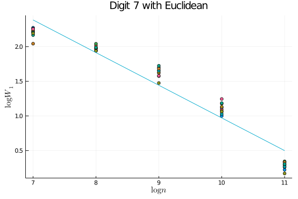
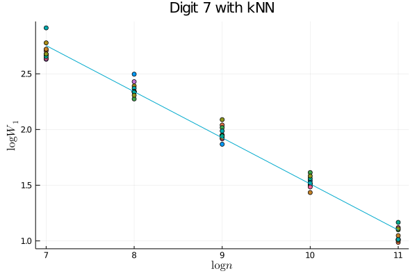
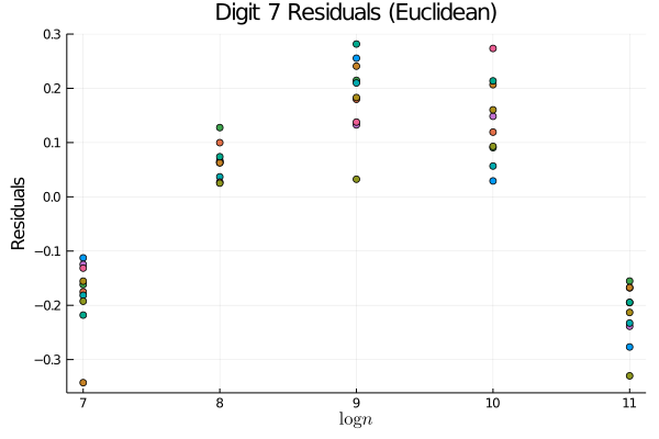
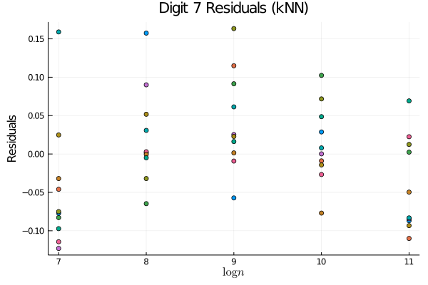
A natural question: is this more complicated approach necessary? i.e., is on real datasets? We believe that the answer is yes. To see this, consider the case of images of the digit 7 (for example) from MNIST (LeCun & Cortes,, 2010). As a demonstration, we sample images from MNIST in datasets of size ranging in powers of 2 from to , calculate the Wasserstein distance between these two samples, and plot the resulting trend. In the right plot, we pool all of the data to estimate the manifold distances, and then use these estimated distances to compute the Wasserstein distance between the empirical distributions. In order to better compare these two approaches, we also plot the residuals to the linear fit that we expect in the asymptotic regime. Looking at Figure 1, it is clear that we are not yet in the asymptotic regime if we simply use Euclidean distances; on the other hand, the trend using the manifold distances is much more clearly linear, suggesting that the slope of the best linear fit is meaningful. Thus we see that in order to get a meaningful dimension estimate from practical data sets, we cannot simply use but must also estimate the geometry of the underlying distribution; this suggests that on this data manifold. More generally, we note that the injectivity radius, , is intrinsic to the geometry of the manifold and thus unaffected by the imbedding; in contradistinction, the reach, , is extrinsic and thus can be made smaller by changing the imbedding. In particular, when the obstruction to the reach being large is a “bottleneck” in the sense that the manifold is imbedded in such a way as to place distant neighborhoods of the manifold close together in Euclidean distance (see Figure 2 for an example), we may expect . Intuitively, this matches the notion that the geometry of the data would be simple if we were to have access to the “correct” coordinate system and that the difficulty in understanding the geometry comes from its imbedding in the ambient space.
We emphasize that, like many estimators of intrinsic dimension, we do not claim robustness to off-manifold noise (Levina & Bickel,, 2004; Farahmand et al.,, 2007; Kim et al.,, 2019). Indeed, any “fattening” of the manifold will force any consistent estimator of intrinsic dimension to asymptotically grow to the full, ambient dimension as the number of samples grows. Various works have included off-manifold noise in different ways, often with the assumption that either the noise is known (Koltchinskii,, 2000) or the manifold is linear (Niles-Weed & Rigollet,, 2019). Methods that do not make these simplifying assumptions are often highly sensitive to scaling parameters that are required inputs in such methods as multi-scale, local SVD (Little et al.,, 2009). Extensions of our method to such noisy settings are a promising avenue of future research, particularly in understanding the effect of this noise on downstream applications as is done for Lipschitz classification in metric spaces and the resulting dimension-distortion tradeoff found in Gottlieb et al., (2016); in this work, however, we confine our theoretical study to the noiseless setting. The primary theoretical advantage of our estimator over that of Levina & Bickel, (2004); Farahmand et al., (2007) is that we do not require the stringent regularity assumptions for our nonasymptotic rates to hold. We leave it for future empirical works whether this weakening of assumptions allows for a better practical estimator on real-world data sets.
Our main contributions are as follows:
-
•
In Section 3, we introduce a new estimator of intrinsic dimension. In Theorem 22 we prove non-asymptotic bounds on the quality of the introduced estimator. Moreover, unlike the MLE estimator of Levina & Bickel, (2004) with non-asymptotic analysis in Farahmand et al., (2007), minimal regularity of the density of the population distribution is required for our guarantees and, unlike that suggested in Kim et al., (2019), our estimator is both computationally efficient and has sample complexity independent of the ambient dimension.
-
•
In the course of proving Theorem 22, we adapt the techniques of Bernstein et al., (2000) to provide new, non-asymptotic bounds on the quality of kNN distance as an estimate of intrinsic distance in Proposition 24, with explicit sample complexity in terms of the reach of the underlying space. To our knowledge, these are the first such non-asymptotic bounds.
We further note that the techniques we develop to prove the non-asymptotic bounds on our dimension estimator also serve to provide new statistical rates in learning Generative Adversarial Networks (GANs) with a Hölder discriminator class:
-
•
We prove in Theorem 25 that if is a Hölder GAN, then the distance between and , as measured by the Hölder IPM, is governed by rates dependent only on the intrinsic dimension of the data, independent of the ambient dimension or the dimension of the feature space. In particular, we prove in great generality that if has intrinsic dimension , then the rate of a Wasserstein GAN is . This improves on the recent work of Schreuder et al., (2020).
The work is presented in the order of the above listed contributions, preceded by a brief section on the geometric preliminaries and prerequisite results. We conclude the introduction by fixing notation and surveying some related work.
Notation:
We fix the following notation. We always let be a probability distribution on and, whenever defined, we let . We reserve for samples taken from and we denote by their empirical distribution. We reserve for the smoothness of a Hölder class, is always a bounded open domain, and is always the intrinsic diameter of a closed set. We also reserve for a compact manifold. In general, we denote by the support of a distribution and we reuse if we restrict ourselves to the case where is a compact manifold, with Riemannian metric induced by the Euclidean metric. We denote by the volume of the manifold with respect to its inherited metric and we reserve for the volume of the unit ball in . When a compact manifold manifold can be assumed from context, we take the uniform measure on to be the volume measure of normalized so that has unit measure.
1.1 Related Work
Dimension Estimation
There is a long history of dimension estimation, beginning with linear methods such as thresholding principal components (Fukunaga & Olsen,, 1971), regressing k-Nearest-Neighbors (kNN) distances (Pettis et al.,, 1979), estimating packing numbers (Kégl,, 2002; Grassberger & Procaccia,, 2004; Camastra & Vinciarelli,, 2002), an estimator based solely on neighborhood (but not metric) information that was recently proven consistent (Kleindessner & Luxburg,, 2015), and many others. An exhaustive recent survey on the history of these techniques can be found in Camastra & Staiano, (2016). Perhaps the most popular choice among current practitioners is the MLE estimator of Levina & Bickel, (2004).
The MLE estimator is constructed as the maximum likelihood of a parameterized Poisson process. As worked out in Levina & Bickel, (2004), a local estimate of dimension for and is given by
where is the distance between and its nearest neighbor in the data set. The final estimate for fixed is given by averaging over the data points in order to reduce variance. While not included in the original paper, a similar motivation for such an estimator could be noting that if is uniformly distributed on a ball of radius in , then ; the local estimator is the empirical version under the assumption that the density is smooth enough to be approximately constant on this small ball. The easy computation is included for the sake of completeness in Appendix E. In Farahmand et al., (2007), the authors examined a closely related estimator and provided non-asymptotic guarantees with an exponential dependence on the intrinsic dimension, albeit with stringent regularity conditions on the density.
In addition to the estimators motivated by the volume growth of local balls discussed in the previous paragraph, Kim et al., (2019) proposed and analyzed a dimension estimator based on Travelling Salesman Paths (TSP). One major advantage to the TSP estimator is the lack of necessary regularity conditions on the density, requiring only an upper bound of the likelihood of the population density with respect to the volume measure on the manifold. On the other hand, the upper bound on sample complexity that that paper presents depends exponentially on the ambient dimension, which is pessimistic when the intrinsic dimension is substantially smaller. In addition, it is unclear how practical the estimator is due to the necessity of computing a solution to TSP; even ignoring this issue, Kim et al., (2019) note that practical tuning of the constants involved in their estimator is difficult and thus deploying their estimator as is on real-world datasets is unlikely.
Manifold Learning
The notion of reach was first introduced in Federer, (1959), and subsequently used in the machine learning and computational geometry communities in such works as Niyogi et al., (2008, 2011); Aamari et al., (2019); Amenta & Bern, (1999); Fefferman et al., (2016, 2018); Narayanan & Mitter, (2010); Efimov et al., (2019); Boissonnat et al., (2019). Perhaps most relevant to our work, Narayanan & Mitter, (2010); Fefferman et al., (2016) consider the problem of testing membership in a class of manifolds of large reach and derive tight bounds on the sample complexity of this question. Our work does not fall into the purview of their conclusions as we assume that the geometry of the underlying manifold is nice and estimate the intrinsic dimension. In the course of proving bounds on our dimension estimator, we must estimate the intrinsic metric of the data. We adapt the proofs of Tenenbaum et al., (2000); Bernstein et al., (2000); Niyogi et al., (2008) and provide tight bounds on the quality of a -Nearest Neighbors (NN) approximation of the intrinsic distance.
Statistical Rates of GANs
Since the introduction of Generative Adversarial Networks (GANs) in Goodfellow et al., (2014), there has been a plethora of empirical improvements and theoretical analyses. Recall that the basic GAN problem selects an estimated distribution from a class of distributions minimizing some adversarially learned distance between and the empirical distribution . Theoretical analyses aim to control the distance between the learned distribution and the population distribution from which the data comprising are sampled. In particular statistical rates for a number of interesting discriminator classes have been proven including Besov balls (Uppal et al.,, 2019), balls in an RKHS (Liang,, 2018), and neural network classes (Chen et al.,, 2020) among others. The latter paper, Chen et al., (2020) also considers GANs where the discriminative class is a Hölder ball, which includes the popular Wasserstein GAN framework of Arjovsky et al., (2017). They show that if is the empirical minimizer of the GAN loss and the population distribution then
up to factors polynomial in . Thus, in order to beat the curse of dimensionality, one requires ; note that the larger is, the weaker the IPM is as the Hölder ball becomes smaller. In order to mitigate this slow rate, Schreuder et al., (2020) assume that both and are distributions arising from Lipschitz pushforwards of the uniform distribution on a -dimensional hypercube; in this setting, they are able to remove dependence on and show that
This last result beats the curse of dimensionality, but pays with restrictive assumptions on the generative model as well as dependence on the Lipschitz constant of the pushforward map. More importantly, the result depends exponentially not on the intrinsic dimension of but rather on the dimension of the feature space used to represent . In practice, state-of-the-art GANs used to produce images often choose to be on the order of , which is much too large for the Schreuder et al., (2020) result to guarantee good performance.
2 Preliminaries
2.1 Geometry
In this work, we are primarily concerned with the case of compact manifolds isometrically imbedded in some large ambient space, . We note that this focus is largely in order to maintain simplicity of notation and exposition; extensions to more complicated, less regular sets with intrinsic dimension defined as the Minkowski dimension can easily be attained with our techniques. The key example to keep in mind is that of image data, where each pixel corresponds to a dimension in the ambient space, but, in reality, the distribution lives on a much smaller, imbedded subspace. Many of our results can be easily extended to the non-compact case with additional assumptions on the geometry of the space and tails of the distribution of interest.
Central to our study is the analysis of how complex the support of a distribution is. We measure complexity of a metric space by its entropy:
Definition 2.
Let be a metric space. The covering number at scale , , is the minimal number such that there exist points such that is contained in the union of balls of radius centred at the . The packing number at scale , , is the maximal number such that there exist points such that for all . The entropy is defined as .
We recall the classical packing-covering duality, proved, for example, in (van Handel,, 2014, Lemma 5.12):
Lemma 3.
For any metric space and scale ,
The most important geometric quantity that determines the complexity of a problem is the dimension of the support of the population distribution. There are many, often equivalent ways to define this quantity in general. One possibility, introduced in Assouad, (1983) and subsequently used in Dasgupta & Freund, (2008); Kpotufe & Dasgupta, (2012); Kpotufe & Garg, (2013) is that of doubling dimension:
Definition 4.
Let be a closed set. For , the doubling dimension at is the smallest such that for all , the set can be covered by balls of radius , where denotes the Euclidean ball of radius centred at . The doubling dimension of is the supremum of the doubling dimension at for all .
This notion of dimension plays well with the entropy, as demonstrated by the following (Kpotufe & Dasgupta,, 2012, Lemma 6):
Lemma 5 ((Kpotufe & Dasgupta,, 2012)).
Let have doubling dimension and diameter . Then .
We remark that a similar notion of dimension is that of the Minkowski dimension, which is defined as the asymptotic rate of growth of the entropy as the scale tends to zero. Recently, Nakada & Imaizumi, (2020) examined the effect that an assumption of small Minkowski dimension has on learning with neural networks; their central statistical result can be recovered as an immediate consequence of our complexity bounds below.
In order to develop non-asymptotic bounds, we need some understanding of the geometry of the support, . We first recall the definition of the geodesic distance:
Definition 6.
Let be closed. A piecewise smooth curve in , , is a continuous function , where is an interval, such that there exists a partition of such that is smooth as a function to . The length of is induced by the imbedding of . For points , the intrinsic (or geodesic) distance is
It is clear from the fact that straight lines are geodesics in that for any points , . We are concerned with two relevant geometric quantities, one extrinsic and the other intrinsic.
Definition 7.
Let be a closed set. Let the medial axis be defined as
In other words, the medial axis is the set of points in that have at least two projections to . Define the reach, of as , the minimal distance between a set and its medial axis.
If is a compact manifold with the induced Euclidean metric, we define the injectivity radius as the maximal such that if such that then there exists a unique length-minimizing geodesic connecting to in .
For more detail on the injectivity radius, see Lee, (2018), especially Chapters 6 and 10. The difference between and is in the choice of metric with which we equip . We could choose to equip with the metric induced by the Euclidean distance or we could choose to use the intrinsic metric defined above. The reach quantifies the maximal radius of a ball with respect to the Euclidean distance such that the intersection of this ball with behaves roughly like Euclidean space. The injectivity radius, meanwhile, quantifies the maximal radius of a ball with respect to the intrinsic distance such that this ball looks like Euclidean space. While neither quantity is necessary for our dimension estimator, both figure heavily in the analysis. The final relevant geometric quantity is the sectional curvature. The sectional curvature of at a point given two directions tangent to at is given by the Gaussian curvature at of the image of the exponential map applied to a small neighborhood of the origin in the plane determined by the two directions. Intuitively, the sectional curvature measures how tightly wound the manifold is locally around each point. For an excellent exposition on the topic, see (Lee,, 2018, Chapter 8).
We now specialize to consider compact, dimension manifolds imbedded in with the induced metric (see Lee, (2018) for an accessible introduction to the geometric notions discussed here). One measure of size of the manifold is the diameter, , with respect to the intrinsic distance defined above. Another notion of size is the volume measure, . This measure can be defined intrinsically as integration with respect to the volume form, where the volume form can be thought of as the analogue of the Lebesgue differential in standard Euclidean space; for more details see Lee, (2018). In our setting, we could equivalently define the volume as the -dimensional Hausdorff measure as in Aamari et al., (2019). Either way, when we refer to a measure that is uniform on the manifold, we consider the normalization such that , i.e., .
With the brief digression into volume concluded, we return to the notion of the reach, which encodes a number of local and global geometric properties. We summarize several of these in the following proposition:
Proposition 8.
Let be a compact manifold isometrically imbedded in . Suppose that . The following hold:
A few remarks are in order. First, note that the Hopf-Rinow Theorem (Hopf & Rinow,, 1931) guarantees that is complete, which is fortuitous as completeness is a necessary, technical requirement for several of our arguments. Second, we note that (c) from Proposition 8 has a simple geometric interpretation: the upper bound on the right hand side is the length of the arc of a circle of radius containing points ; thus, the maximal distortion of the intrinsic metric with respect to the ambient metric is bounded by the circle of radius .
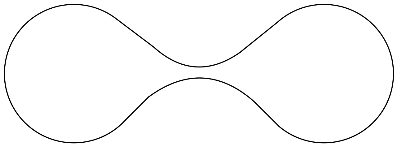
Point (a) in the above proposition demonstrates that control of the reach leads to control of local distortion. From the definition, it is obvious that the reach provides an upper bound for the size of the global notion of a “bottleneck,” i.e., two points such that . Interestingly, these two local and global notions of distortion are the only ways that the reach of a manifold can be small, as (Aamari et al.,, 2019, Theorem 3.4) tells us that if the reach of a manifold is , then either there exists a bottleneck of size or the norm of the second fundamental form is at some point. Thus, in some sense, the reach is the “correct” measure of distortion. Note that while (b) above tells us that , there is no comparable upper bound. To see this, consider Figure 2, which depicts a one-dimensional manifold imbedded in . Note that the bottleneck in the center ensures that the reach of this manifold is very small; on the other hand, it is easy to see that the injectivity radius is given by half the length of the entire curve. As the curve can be extended arbitrarily, the reach can be arbitrarily small relative to the injectivity radius.
We now proceed to bound the covering number of a compact manifold using the dimension and the injectivity radius. We note that upper bounds on the covering number with respect to the ambient metric were provided in Niyogi et al., (2008); Narayanan & Mitter, (2010). A similar bound with less explicit constants can be found in (Kim et al.,, 2019, Lemma 4).
Proposition 9.
Let be an isometrically imbedded, compact, -dimensional submanifold with injectivity radius such that the sectional curvatures are bounded above by and below by . If then
If then
Moreover, for all ,
Thus, if , where is the reach of , then
The proof of Proposition 9 can be found in Appendix A and relies on the Bishop-Gromov comparison theorem to leverage the curvature bounds from Proposition 8 into volume estimates for small intrinsic balls, a similar technique as found in Niyogi et al., (2008); Narayanan & Mitter, (2010). The key point to note is that we have both upper and lower bounds for , as opposed to just the upper bound guaranteed by Lemma 5. As a corollary, we are also able to derive bounds for the covering number with respect to the ambient metric:
Corollary 10.
Let be as in Proposition 9. For , we can control the covering numbers of with respect to the Euclidean metric as
2.2 Hölder Classes and their Complexity
In this section we make the elementary observation that complex function classes restricted to simple subsets can be much smaller than the original class. While such intuition has certainly appeared before, especially in designing esimators that can adapt to local intrinsic dimension, such as Bickel et al., (2007); Kpotufe & Dasgupta, (2012); Kpotufe, (2011); Kpotufe & Garg, (2013); Dasgupta & Freund, (2008); Steinwart et al., (2009); Nakada & Imaizumi, (2020), we codify this approach below.
To illustrate the above phenomenon at the level of empirical processes, we focus on Hölder functions in for some large and let the “simple” subset be a subspace of dimension where . We first recall the definition of a Hölder class:
Definition 11.
For an open domain and a function , define the -Hölder norm as
Define the Hölder ball of radius , denoted by , as the set of functions such that . If is a Riemannian manifold of class (see Lee, (2018)), and we define the Hölder norm analogously, replacing with , where is the covariant derivative.
It is a classical result of Kolmogorov & Tikhomirov, (1993) that, for a bounded, open domain , the entropy of a Hölder ball scales as
as . As a consequence, we arrive at the following result, whose proof can be found in Appendix A for the sake of completeness.
Proposition 12.
Let be a path-connected closed set contained in an open domain . Let and let . Then,
Note that the content of the above result is really that of Kolmogorov & Tikhomirov, (1993), coupled with the fact that restriction from to preserves smoothness.
If we apply the easily proven volumetric bounds on covering and packing numbers for a Euclidean ball to Proposition 12, we recover the classical result of Kolmogorov & Tikhomirov, (1993). The key insight is that low-dimensional subsets can have covering numbers much smaller than those of a high-dimensional Euclidean ball: if the “dimension” of is , then we expect the covering number of to scale like . Plugging this into Proposition 12 tells us that the entropy of , up to a factor logarithmic in , scales like . An immediate corollary of Lemma 5 and Proposition 12 is:
Corollary 13.
Let be a closed set of diameter and doubling dimension . Let open and be the restriction of to . Then
The conclusion of Corollary 13 is very useful for upper bounds as it tells us that the entropy for Hölder balls scales at most like as . If we desire comparable lower bounds, we require some of the geometry discussed above. Combining Proposition 12 and Corollary 10 yields the following bound:
Corollary 14.
Let be an isometrically imbedded, compact submanifold with reach and let . Suppose is an open set and let be the restriction of to . Then for ,
If we set , then we have that for all ,
In essence, Corollary 14 tells us that the rate of for the growth of the entropy of Hölder balls is sharp for sufficiently small . The key difference between the first and second statements is that the first is with respect to an ambient class of functions while the second is with respect to an intrinsic class. To better illustrate the difference, consider the case where , i.e., the class of Lipschitz functions on the manifold. In both cases, asymptotically, the entropy of Lipschitz functions scales like ; if we restrict to functions that are Lipschitz with respect to the ambient metric, then the above bound only applies for ; on the other hand, if we consider the larger class of functions that are Lipschitz with respect to the intrinsic metric, the bound applies for . In the case where , this can be a major improvement.
The observations in this section are undeniably simple; the real interest comes in the diverse applications of the general principle, some of which we detail below. As a final note, we remark that our guiding principle of simplifying function classes by restricting them to simple sets likely holds in far greater analysis than is explored here; in particular, Sobolev and Besov classes (see, for example, (Giné & Nickl,, 2016, §4.3)) likely exhibit similar behavior.
3 Dimension Estimation
We outlined the intuition behind our dimension estimation in the introduction. In this section, we formally define the estimator and analyse its theoretical performance. We first apply standard empirical process theory and our complexity bounds in the previous section to upper bound the expected Hölder IPM (defined in (1)) between empirical and population distributions:
Lemma 15.
Let be a compact set contained in a ball of radius . Suppose that we draw independent samples from a probability measure supported on and denote by the corresponding empirical distribution. Let denote an independent identically distributed measure as . Then we have
In particular, there exists a universal constant such that if for some , then
holds with .
The proof uses the symmetrization and chaining technique and applies the complexity bounds of Hölder functions found above; the details can be found in Appendix E.
We now specialize to the case where , due to the computational tractability of the resulting Wasserstein distance. Applying Kantorovich-Rubenstein duality (Kantorovich & Rubinshtein,, 1958), we see that this special case of Lemma 15 recovers the special case of Weed et al., (2019). From here on, we suppose that and our metric on distributions is .
We begin by noting that if we have , independent samples from , then we can split them into two data sets of size , and denote by the empirical distributions thus generated. We then note that Lemma 15 implies that if and is of dimension , then
If we were to establish a lower bound as well as concentration of about its mean, then we could consider the following estimator. Given a data set of size , we can break the data into four samples, each of size and of size . Then we would have
Which distance on should be used to compute the Wasserstein distance, the Euclidean metric or the intrinsic metric ? As can be guessed from Corollary 14, asymptotically, both will work, but for finite sample sizes when , the latter is much better. One problem remains, however: because we are not assuming to be known, we do not have access to and thus we cannot compute the necessary Wasserstein cost. In order to get around this obstacle, we recall the graph distance induced by a NN graph:
Definition 16.
Let be a data set and fix . We let denote the weighted graph with vertices and edges of weight between all vertices such that . We denote by (or if are clear from context) the geodesic distance on the graph . We extend this metric to all of by letting
where .
We now have two Wasserstein distances, each induced by a different metric; to mitigate confusion, we introduce the following notation:
Definition 17.
Let , sampled independently from such that . Let be the empirical distributions associated to the data . Let denote the Wasserstein cost with respect to the Euclidean metric and denote the Wasserstein cost associated to the manifold metric, as in (1). For a fixed , let denote the Wasserstein cost associated to the metric . Let , , and denote the dimension estimators from (3) induced by each of the above metrics.
Given sample distributions , we are able to compute and for any fixed , but not because we are assuming that the learner does not have access to the manifold . On the other hand, adapting techniques from Weed et al., (2019), we are able to provide a non-asymptotic lower bound on and :
Proposition 18.
Suppose that is a measure on such that , where is a -dimensional, compact manifold with reach and such that the density of with respect to the uniform measure on is lower bounded by . Suppose that
Then, almost surely,
If we assume only that
then, almost surely,
An easy proof, based on the techniques (Weed et al.,, 2019, Proposition 6) can be found in Appendix E. Similarly, we can apply the same proof technique as Lemma 15 to establish the following upper bound:
Proposition 19.
Let be a compact manifold with positive reach and dimension . Furthermore, suppose that is a probability measure on with . Let be independent with corresponding empirical distributions . Then if , we have:
The full proof is in Appendix E and applies symmetrization and chaining, with an upper bound of Corollary 14. We note, as before, that a similar asymptotic rate is obtained by Weed et al., (2019) in a slightly different setting.
We noted above (3) that we required two facts to make our intuition precise. We have just shown that the first holds; we turn now to the second: concentration. To make this rigorous, we need one last technical concept: the -inequality.
Definition 20.
Let be a measure on a metric space . We say that satisfies a -inequality with constant if for all measures , we have
where is the well-known KL-divergence.
The reason that the inequality is useful for us is that Bobkov & Götze, (1999) tell us that such an inequality implies, and is, by Gozlan et al., (2009), equivalent to Lipschitz concentration. We note further that is a Lipschitz function of the dataset and thus concentrates about its mean. The constant in the inequality depends on the measure and upper bounds for specific classes of measures are both well-known and remain an active area of research; for a more complete survey, see Bakry et al., (2014). We have the following bound:
Proposition 21.
Let be a probability measure on that has density with respect to the (normalized) volume measure of , lower bounded by and upper bounded by , where is a -dimensional manifold with reach and . Then we have:
| (3) |
In order to bound the constant in our case, we rely on the landmark result of Otto & Villani, (2000) that relates to another functional inequality, the log-Sobolev inequality (Bakry et al.,, 2014, Chapter 5). There are many ways to control the log-Sobolev constant in various situations, many of which are covered in Bakry et al., (2014). We use results from Wang, (1997b), which incorporate the intrinsic geometry of the distribution, as our bound. A detailed proof can be found in Appendix B. We note that many other estimates with under slightly different conditions exits, such as that in Wang, (1997a), which requires second-order control of the density of the population distribution with respect to the volume measure and the bound in Block et al., (2020), which provides control using a measure of nonconvexity. With added assumptions, we can gain much sharper control over ; for example, if we assume a positive lower bound on the curvature of the support, we can apply the well-known Bakry-Émery result (Bakry & Émery,, 1985) and get dimension-free bounds. As another example, if we may assume stronger contol on the curvature of beyond that guaranteed by the reach, we can remove the exponential dependence on the reach entirely. For the sake of simplicity and because we already admit an exponential dependence on the intrinsic dimension, we present only the more general bound here. We now provide a non-asymptotic bound on the quality of the estimator .
Theorem 22.
Let be a probability measure on and suppose that has a density with respect to the (normalized) volume measure of lower bounded by , where is a -dimensional manifold with reach such that and . Furthermore, suppose that satisfies a inequality with constant . Let and suppose satisfy
Suppose we have samples drawn independently from . Then, with probability at least , we have
If is replaced by above, we get the same bound with the vanilla estimator replacing .
We note that we have not made every effort to minimize the constants in the statement above, with our emphasis being the dependence of these sample complexity bounds on the relevant geometric quantities. As an immediate consequence of Theorem 22, due to the fact that is discrete, we can control the probability of error with sufficiently many samples. We may also apply Proposition 21 to replace with our upper bound in terms of the reach.
Corollary 23.
Suppose we are in the situation of Theorem 22 and that has density upper bounded by with respect to the normalized uniform measure on . Suppose further that satisfy
Then if we round to the nearest integer, and denote the resulting estimator by , we have with probability at least , . Again, replacing by in the previous display yields the same result with replaced by the vanilla estimator .
Proof.
While the appearance of in Theorem 22 and Corollary 23 may seem minor, it is critical for any practical estimator. While , we may take as small as . Thus, using instead of the naive estimator allows us to leverage the entire data set in estimating the intrinsic distances, even on the small sub-samples. From the proof, it is clear that we want to be as large as possible; thus if we have a total of samples, we wish to make as small as possible. If then we can make much smaller (scaling like ) than if we were to simply use the Euclidean distance. As a result, on any data set where , the sample complexity of can be much smaller than that of .
There are two parts to the proof of Theorem 22: first, we need to establish that our metric approximates with high probability and thus ; second, we need to show that is, indeed, a good estimate of . The second part follows from Propositions 19 and 18, and concentration; a detailed proof can be found in Appendix C. For the first part of the proof, in order to show that , we demonstrate that in the following result:
Proposition 24.
Let be a probability measure on and suppose that , a geodesically convex, compact manifold of dimension and reach . Suppose that we sample independently. Let and . If for some ,
where for any
with the metric ball around of radius . Then, with probability at least , for all ,
The proof of Proposition 24 follows the general outline of Bernstein et al., (2000), but is modified in two key ways: first, we control relevant geometric quantities by instead of by the quantities in Bernstein et al., (2000); second, we provide a quantitative, nonasymptotic bound on the number of samples needed to get a good approximation with high probability. The details are deferred to Appendix D.
This result may be of interest in its own right as it provides a non-asymptotic version of the results from Tenenbaum et al., (2000); Bernstein et al., (2000). In particular, if we suppose that has a density with respect to the uniform measure on and this density is bounded below by a constant , then Proposition 24 combined with Proposition 9 tells us that if we have
samples, then we can recover the intrinsic distance of with distortion . We further note that the dependence on is quite reasonable in Proposition 24. The argument requires the construction of a -net on and it is not difficult to see that one needs a covering at scale proportional to in order to recover the intrinsic metric from discrete data points. For example, consider Figure 2; were a curve to be added to connect the points at the bottleneck, this would drastically decrease the intrinsic distance between the bottleneck points. In order to determine that the intrinsic distance between these points (without the connector) is actually quite large using the graph metric estimator, we need to set , in which case these points are certainly only connected if there exists a point of distance less than to the bottleneck point, which can only occur with high probability if . We can extend this example to arbitrary dimension by taking the product of the curve with for ; in this case, a similar argument holds and we now need points in order to guarantee with high probability that there exists a point of distance at most to one of the bottleneck points. In this way, we see that the scaling is unavoidable in general. Note that the other estimators of intrinsic dimension mentioned in the introduction, in particular the MLE estimator of Levina & Bickel, (2004), implicitly require the accuracy of the NN distance for their estimation to hold; thus these estimators also suffer from the sample complexity. Finally, we remark that Kim et al., (2019) presents a minimax lower bound for a related hypothesis testing problem and shows that minimax risk is bounded below by a local analogue of the reach raised to a power that depends linearly on the intrinsic dimension.
4 Application of Techniques to GANs
In this section, we note that our techniques are not confined to the realm of dimension estimation and, in fact, readily apply to other problems. As an example, consider the unsupervised learning problem of generative modeling, where we suppose that there are samples independent and we wish to produce a sample such that and are close. Statistically, this problem can be expressed by fixing a class of distributions and using the data to choose such that is in some sense close to . For computational reasons, one wishes to contain distributions from which it is computationally efficient to sample; in practice, is usually the class of pushforwards of a multi-variate Gaussian distribution by some deep neural network class . While our statistical results include this setting, they are not restricted and apply for general classes of distributions .
In order to make the problem more precise, we require some notion of distance between distributions. We use the notion of the Integral Probability Metric (Müller,, 1997; Sriperumbudur et al.,, 2012) associated to a Hölder ball , as defined above. We suppose that and we abbreviate the corresponding IPM distance by . Given the empirical distribution , the GAN that we study can be expressed as
In this section, we generalize the results of Schreuder et al., (2020). In particular, we derive new estimation rates for a GAN using a Hölder ball as a discriminating class, assuming that the population distribution is low-dimensional; like Schreuder et al., (2020), we consider the noised and potentially contaminated setting. We have
Theorem 25.
Suppose that is a probability measure on supported on a compact set and suppose we have independent with empirical distribution . Let be independent, centred random variables on such that . Suppose we observe such that for at least of the , we have ; let the empirical distribution of the be . Let be a known set of distributions and define
Then if there is some such that , we have
where is a constant depending linearly on .
We note that the factor can be easily removed for all cases by paying slightly in order to increase the constants; for the sake of simplicity, we do not bother with this argument here. The proof of Theorem 25 is similar in spirit to that of Schreuder et al., (2020), which in turn follows Liang, (2018), with details in Appendix E. The key step is in applying the bounds in Lemma 15 to the arguments of Liang, (2018).
We compare our result to the corresponding theorem (Schreuder et al.,, 2020, Theorem 2). In that work, the authors considered a setting where there is a known intrinsic dimension and the population distribution , the push-forward by an -Lipschitz function of the uniform distribution on a -dimensional hypercube; in addition, they take to be the set of push-forwards of by functions in some class , all of whose elements are -Lipschitz. Their result, (Schreuder et al.,, 2020, Theorem 2), gives an upper bound of
| (4) |
Note that our result is an improvement in two key respects. First, we do not treat the intrinsic dimension as known, nor do we force the dimension of the feature space to be the same as the intrinsic dimension. Many of the state-of-the-art GAN architectures on datasets such as ImageNet use a feature space of dimension 128 or 256 (Wu et al.,, 2019); the best rate that the work of Schreuder et al., (2020) can give, then would be . In our setting, even if the feature space is complex, if the true distribution lies on a much lower dimensional subspace, then it is the true, intrinsic dimension, that determines the rate of estimation. Secondly, note that the upper bound in (4) depends on the Lipschitz constant ; as the function classes used to determine the push-forwards are essentially all deep neural networks in practice, and the Lipschitz constants of such functions are exponential in depth, this can be a very pessimistic upper bound; our result, however, does not depend on this Lipschitz constant, but rather on properties intrinsic to the probability distribution . This dependence is particularly notable in the noisy regime, where do not vanish; the large multiplicative factor of in this case would then make the bound useless.
We conclude this section by considering the case most often used in practice: the Wasserstein GAN.
Corollary 26.
Suppose we are in the setting of Theorem 25 and is contained in a ball of radius for . Then,
The proof of the corollary is almost immediate from Theorem 25. With additional assumptions on the tails of the , we can turn our expectation into a high probability statement. In the special case with neither noise nor contamination, i.e. , we get that the Wasserstein GAN converges in Wasserstein distance at a rate of , which we believe explains in large part the recent empirical success in modern Wasserstein-GANs.
Acknowledgements
We acknowledge support from the NSF through award DMS-2031883 and from the Simons Foundation through Award 814639 for the Collaboration on the Theoretical Foundations of Deep Learning. We acknowledge the support from NSF under award DMS-1953181, NSF Graduate Research Fellowship support under Grant No. 1122374, and support from the MIT-IBM Watson AI Lab.
References
- Aamari et al., (2019) Aamari, Eddie, Kim, Jisu, Chazal, Frédéric, Michel, Bertrand, Rinaldo, Alessandro, Wasserman, Larry, et al. 2019. Estimating the reach of a manifold. Electronic journal of statistics, 13(1), 1359–1399.
- Amenta & Bern, (1999) Amenta, Nina, & Bern, Marshall. 1999. Surface reconstruction by Voronoi filtering. Discrete & Computational Geometry, 22(4), 481–504.
- Arjovsky et al., (2017) Arjovsky, Martin, Chintala, Soumith, & Bottou, Léon. 2017. Wasserstein generative adversarial networks. Pages 214–223 of: International conference on machine learning. PMLR.
- Ashlagi et al., (2021) Ashlagi, Yair, Gottlieb, Lee-Ad, & Kontorovich, Aryeh. 2021. Functions with average smoothness: structure, algorithms, and learning. Pages 186–236 of: Conference on Learning Theory. PMLR.
- Assouad, (1983) Assouad, Patrice. 1983. Plongements lipschitziens dans . Bulletin de la Société Mathématique de France, 111, 429–448.
- Bakry & Émery, (1985) Bakry, Dominique, & Émery, Michel. 1985. Diffusions hypercontractives. Pages 177–206 of: Seminaire de probabilités XIX 1983/84. Springer.
- Bakry et al., (2014) Bakry, Dominique, Gentil, Ivan, & Ledoux, Michel. 2014. Analysis and Geometry of Markov Diffusion Operators. Springer International Publishing.
- Belkin & Niyogi, (2001) Belkin, Mikhail, & Niyogi, Partha. 2001. Laplacian eigenmaps and spectral techniques for embedding and clustering. Pages 585–591 of: Nips, vol. 14.
- Bernstein et al., (2000) Bernstein, Mira, Silva, Vin De, Langford, John C., & Tenenbaum, Joshua B. 2000. Graph Approximations to Geodesics on Embedded Manifolds.
- Bickel et al., (2007) Bickel, Peter J, Li, Bo, et al. 2007. Local polynomial regression on unknown manifolds. Pages 177–186 of: Complex datasets and inverse problems. Institute of Mathematical Statistics.
- Block et al., (2020) Block, Adam, Mroueh, Youssef, Rakhlin, Alexander, & Ross, Jerret. 2020. Fast mixing of multi-scale langevin dynamics underthe manifold hypothesis. arXiv preprint arXiv:2006.11166.
- Bobkov & Götze, (1999) Bobkov, Sergej G, & Götze, Friedrich. 1999. Exponential integrability and transportation cost related to logarithmic Sobolev inequalities. Journal of Functional Analysis, 163(1), 1–28.
- Boissonnat et al., (2019) Boissonnat, Jean-Daniel, Lieutier, André, & Wintraecken, Mathijs. 2019. The reach, metric distortion, geodesic convexity and the variation of tangent spaces. Journal of applied and computational topology, 3(1), 29–58.
- Camastra & Staiano, (2016) Camastra, Francesco, & Staiano, Antonino. 2016. Intrinsic dimension estimation: Advances and open problems. Information Sciences, 328, 26–41.
- Camastra & Vinciarelli, (2002) Camastra, Francesco, & Vinciarelli, Alessandro. 2002. Estimating the intrinsic dimension of data with a fractal-based method. IEEE Transactions on pattern analysis and machine intelligence, 24(10), 1404–1407.
- Chen et al., (2020) Chen, Minshuo, Liao, Wenjing, Zha, Hongyuan, & Zhao, Tuo. 2020. Statistical Guarantees of Generative Adversarial Networks for Distribution Estimation.
- Cuturi, (2013) Cuturi, Marco. 2013. Sinkhorn distances: Lightspeed computation of optimal transport. Pages 2292–2300 of: Advances in neural information processing systems.
- Dasgupta & Freund, (2008) Dasgupta, Sanjoy, & Freund, Yoav. 2008. Random projection trees and low dimensional manifolds. Pages 537–546 of: Proceedings of the fortieth annual ACM symposium on Theory of computing.
- Donoho & Grimes, (2003) Donoho, David L, & Grimes, Carrie. 2003. Hessian eigenmaps: Locally linear embedding techniques for high-dimensional data. Proceedings of the National Academy of Sciences, 100(10), 5591–5596.
- Dudley, (1969) Dudley, Richard Mansfield. 1969. The speed of mean Glivenko-Cantelli convergence. The Annals of Mathematical Statistics, 40(1), 40–50.
- Efimov et al., (2019) Efimov, Kirill, Adamyan, Larisa, & Spokoiny, Vladimir. 2019. Adaptive nonparametric clustering. IEEE Transactions on Information Theory, 65(8), 4875–4892.
- Farahmand et al., (2007) Farahmand, Amir Massoud, Szepesvári, Csaba, & Audibert, Jean-Yves. 2007. Manifold-adaptive dimension estimation. Pages 265–272 of: Proceedings of the 24th international conference on Machine learning.
- Federer, (1959) Federer, Herbert. 1959. Curvature measures. Transactions of the American Mathematical Society, 93(3), 418–491.
- Fefferman et al., (2016) Fefferman, Charles, Mitter, Sanjoy, & Narayanan, Hariharan. 2016. Testing the manifold hypothesis. Journal of the American Mathematical Society, 29(4), 983–1049.
- Fefferman et al., (2018) Fefferman, Charles, Ivanov, Sergei, Kurylev, Yaroslav, Lassas, Matti, & Narayanan, Hariharan. 2018. Fitting a putative manifold to noisy data. Pages 688–720 of: Conference On Learning Theory. PMLR.
- Fukunaga & Olsen, (1971) Fukunaga, Keinosuke, & Olsen, David R. 1971. An algorithm for finding intrinsic dimensionality of data. IEEE Transactions on Computers, 100(2), 176–183.
- Gigli & Ledoux, (2013) Gigli, Nicola, & Ledoux, Michel. 2013. From log Sobolev to Talagrand: a quick proof. Discrete and Continuous Dynamical Systems-Series A, dcds–2013.
- Giné & Nickl, (2016) Giné, Evarist, & Nickl, Richard. 2016. Mathematical foundations of infinite-dimensional statistical models. Cambridge University Press.
- Goodfellow et al., (2014) Goodfellow, Ian J, Pouget-Abadie, Jean, Mirza, Mehdi, Xu, Bing, Warde-Farley, David, Ozair, Sherjil, Courville, Aaron, & Bengio, Yoshua. 2014. Generative adversarial networks. arXiv preprint arXiv:1406.2661.
- Gottlieb et al., (2016) Gottlieb, Lee-Ad, Kontorovich, Aryeh, & Krauthgamer, Robert. 2016. Adaptive metric dimensionality reduction. Theoretical Computer Science, 620, 105–118.
- Gozlan et al., (2009) Gozlan, Nathael, et al. 2009. A characterization of dimension free concentration in terms of transportation inequalities. The Annals of Probability, 37(6), 2480–2498.
- Grassberger & Procaccia, (2004) Grassberger, Peter, & Procaccia, Itamar. 2004. Measuring the strangeness of strange attractors. Pages 170–189 of: The Theory of Chaotic Attractors. Springer.
- Gray, (2004) Gray, Alfred. 2004. Tubes. Birkhäuser Basel.
- Holley & Stroock, (1986) Holley, Richard, & Stroock, Daniel W. 1986. Logarithmic Sobolev inequalities and stochastic Ising models.
- Hopf & Rinow, (1931) Hopf, Heinz, & Rinow, Willi. 1931. Über den Begriff der vollständigen differentialgeometrischen Fläche. Commentarii Mathematici Helvetici, 3(1), 209–225.
- Kantorovich & Rubinshtein, (1958) Kantorovich, Leonid Vitaliyevich, & Rubinshtein, SG. 1958. On a space of totally additive functions. Vestnik of the St. Petersburg University: Mathematics, 13(7), 52–59.
- Kégl, (2002) Kégl, Balázs. 2002. Intrinsic dimension estimation using packing numbers. Pages 681–688 of: NIPS. Citeseer.
- Kim et al., (2019) Kim, Jisu, Rinaldo, Alessandro, & Wasserman, Larry. 2019. Minimax Rates for Estimating the Dimension of a Manifold. Journal of Computational Geometry, 10(1).
- Kleindessner & Luxburg, (2015) Kleindessner, Matthäus, & Luxburg, Ulrike. 2015. Dimensionality estimation without distances. Pages 471–479 of: Artificial Intelligence and Statistics. PMLR.
- Kolmogorov & Tikhomirov, (1993) Kolmogorov, A. N., & Tikhomirov, V. M. 1993. epsilon-Entropy and epsilon-Capacity of Sets In Functional Spaces. Pages 86–170 of: Mathematics and Its Applications. Springer Netherlands.
- Koltchinskii, (2000) Koltchinskii, Vladimir I. 2000. Empirical geometry of multivariate data: a deconvolution approach. Annals of statistics, 591–629.
- Kpotufe, (2011) Kpotufe, Samory. 2011. k-NN regression adapts to local intrinsic dimension. Pages 729–737 of: Proceedings of the 24th International Conference on Neural Information Processing Systems.
- Kpotufe & Dasgupta, (2012) Kpotufe, Samory, & Dasgupta, Sanjoy. 2012. A tree-based regressor that adapts to intrinsic dimension. Journal of Computer and System Sciences, 78(5), 1496–1515.
- Kpotufe & Garg, (2013) Kpotufe, Samory, & Garg, Vikas K. 2013. Adaptivity to Local Smoothness and Dimension in Kernel Regression. Pages 3075–3083 of: NIPS.
- LeCun & Cortes, (2010) LeCun, Yann, & Cortes, Corinna. 2010. MNIST handwritten digit database.
- Lee, (2018) Lee, John M. 2018. Introduction to Riemannian manifolds. Springer.
- Levina & Bickel, (2004) Levina, Elizaveta, & Bickel, Peter. 2004. Maximum likelihood estimation of intrinsic dimension. Advances in neural information processing systems, 17, 777–784.
- Liang, (2018) Liang, Tengyuan. 2018. On how well generative adversarial networks learn densities: Nonparametric and parametric results. arXiv preprint arXiv:1811.03179.
- Little et al., (2009) Little, Anna V, Jung, Yoon-Mo, & Maggioni, Mauro. 2009. Multiscale estimation of intrinsic dimensionality of data sets. In: 2009 AAAI Fall Symposium Series.
- Müller, (1997) Müller, Alfred. 1997. Integral probability metrics and their generating classes of functions. Advances in Applied Probability, 429–443.
- Nakada & Imaizumi, (2020) Nakada, Ryumei, & Imaizumi, Masaaki. 2020. Adaptive Approximation and Generalization of Deep Neural Network with Intrinsic Dimensionality. Journal of Machine Learning Research, 21(174), 1–38.
- Narayanan & Mitter, (2010) Narayanan, Hariharan, & Mitter, Sanjoy. 2010. Sample complexity of testing the manifold hypothesis. Pages 1786–1794 of: Proceedings of the 23rd International Conference on Neural Information Processing Systems-Volume 2.
- Niles-Weed & Rigollet, (2019) Niles-Weed, Jonathan, & Rigollet, Philippe. 2019. Estimation of wasserstein distances in the spiked transport model. arXiv preprint arXiv:1909.07513.
- Niyogi et al., (2008) Niyogi, Partha, Smale, Stephen, & Weinberger, Shmuel. 2008. Finding the homology of submanifolds with high confidence from random samples. Discrete & Computational Geometry, 39(1-3), 419–441.
- Niyogi et al., (2011) Niyogi, Partha, Smale, Stephen, & Weinberger, Shmuel. 2011. A topological view of unsupervised learning from noisy data. SIAM Journal on Computing, 40(3), 646–663.
- Otto & Villani, (2000) Otto, Felix, & Villani, Cédric. 2000. Generalization of an inequality by Talagrand and links with the logarithmic Sobolev inequality. Journal of Functional Analysis, 173(2), 361–400.
- Pettis et al., (1979) Pettis, Karl W, Bailey, Thomas A, Jain, Anil K, & Dubes, Richard C. 1979. An intrinsic dimensionality estimator from near-neighbor information. IEEE Transactions on pattern analysis and machine intelligence, 25–37.
- Roweis & Saul, (2000) Roweis, Sam T, & Saul, Lawrence K. 2000. Nonlinear dimensionality reduction by locally linear embedding. science, 290(5500), 2323–2326.
- Schreuder et al., (2020) Schreuder, Nicolas, Brunel, Victor-Emmanuel, & Dalalyan, Arnak. 2020. Statistical guarantees for generative models without domination. arXiv preprint arXiv:2010.09237.
- Sriperumbudur et al., (2012) Sriperumbudur, Bharath K, Fukumizu, Kenji, Gretton, Arthur, Schölkopf, Bernhard, Lanckriet, Gert RG, et al. 2012. On the empirical estimation of integral probability metrics. Electronic Journal of Statistics, 6, 1550–1599.
- Steinwart et al., (2009) Steinwart, Ingo, Hush, Don R, Scovel, Clint, et al. 2009. Optimal Rates for Regularized Least Squares Regression. Pages 79–93 of: COLT.
- Tenenbaum et al., (2000) Tenenbaum, Joshua B, De Silva, Vin, & Langford, John C. 2000. A global geometric framework for nonlinear dimensionality reduction. science, 290(5500), 2319–2323.
- Uppal et al., (2019) Uppal, Ananya, Singh, Shashank, & Póczos, Barnabás. 2019. Nonparametric density estimation & convergence rates for gans under besov ipm losses. arXiv preprint arXiv:1902.03511.
- van Handel, (2014) van Handel, Ramon. 2014. Probability in high dimension. Tech. rept. PRINCETON UNIV NJ.
- Villani, (2008) Villani, Cédric. 2008. Optimal transport: old and new. Vol. 338. Springer Science & Business Media.
- Wang, (1997a) Wang, Feng-Yu. 1997a. Logarithmic Sobolev inequalities on noncompact Riemannian manifolds. Probability theory and related fields, 109(3), 417–424.
- Wang, (1997b) Wang, Feng-Yu. 1997b. On estimation of the logarithmic Sobolev constant and gradient estimates of heat semigroups. Probability theory and related fields, 108(1), 87–101.
- Weed et al., (2019) Weed, Jonathan, Bach, Francis, et al. 2019. Sharp asymptotic and finite-sample rates of convergence of empirical measures in Wasserstein distance. Bernoulli, 25(4A), 2620–2648.
- Wu et al., (2019) Wu, Yan, Donahue, Jeff, Balduzzi, David, Simonyan, Karen, & Lillicrap, Timothy. 2019. Logan: Latent optimisation for generative adversarial networks. arXiv preprint arXiv:1912.00953.
Appendix A Proofs from Section 2
Proof of Proposition 12.
We apply the method from the classic paper (Kolmogorov & Tikhomirov,, 1993), following notation introduced there as applicable. For the sake of simplicity, we assume that is an integer; the generalization to is analogous to that in Kolmogorov & Tikhomirov, (1993). Let and let be a -connected net on . For and , define
where is the norm on tensors induced by the ambient (Euclidean) metric and is the application of the covariant derivative. Let be the matrix of all and let be the set of all such that . Then the argument in the proof of (Kolmogorov & Tikhomirov,, 1993, Theorem XIV) applies mutatis mutandis and we note that are neighborhoods in the Hölder norm. Thus it suffices to bound the number of possible . As in Kolmogorov & Tikhomirov, (1993), we note that the number of possible values for is at most . Given the row , there are at most values for the next row. Thus the total number of possible is bounded by
By definition of the covering number and the fact that is path-connected, we may take
Taking logarithms and noting that concludes the proof of the upper bound.
The middle inequality is Lemma 3. For the lower bound, we again follow Kolmogorov & Tikhomirov, (1993). Define
with a constant to be set. Choose a -separated set with and consider the set of functions
where and varies over all possible sets of signs. The results of Kolmogorov & Tikhomirov, (1993) guarantee that the form a -separated set in if is chosen such that and there are such combinations. By definition of packing numbers, we may choose
This concludes the proof of the lower bound. ∎
Proof of Proposition 9.
We note first that the second statement follows from the first by applying (b) and (c) to Proposition 8 to control the curvature and injectivity radius in terms of the reach. Furthermore, the middle inequality in the last statement follows from Lemma 3. Thus we prove the first two statements.
A volume argument yields the following control:
where is the ball around of radius with respect to the metric . Thus it suffices to lower bound the volume of such a ball. Because , we may apply the Bishop-Gromov comparison theorem (Gray,, 2004, Theorem 3.17) to get that
where is an upper bound on the sectional curvature. We note that for , we have and thus
The upper bound follows from control on the sectional curvature by , appearing in (Aamari et al.,, 2019, Proposition A.1), which, in turn, is an easy consequence of applying the Gauss formula to (a) of Proposition 8.
We lower bound the packing number through an analogous argument as the upper bound for the covering number, this time with an upper bound on the volume of a ball of radius , again from (Gray,, 2004, Theorem 3.17), but this time using a lower bound on the sectional curvature. In particular, we have for ,
where is a lower bound on the sectional curvature. Note that for , we have
Thus,
The volume argument tells us that
and the result follows.
If we wish to extend the range of , we pay with a constant exponential exponential in , reflecting the growth in volume of balls in negatively curved spaces. In particular, we can apply the same argument and note that as is increasing, we have
for all . Thus for all . We have:
as desired. ∎
Proof of Corollary 10.
Let be the set of points in with Euclidean distance to less than and let be the set of points in with intrinsic (geodesic) distance to less than . Then, if , combining the fact that straight lines are geodesics in and (d) from Proposition 8 gives
In particular, this implies
whenever . Thus, applying Proposition 9, we have
and similarly,
using the fact that for . The result follows. ∎
Appendix B Proof of Proposition 21
As stated in the body, we bound the constant by the log-Sobolev constant of the same measure. We thus first define a log-Sobolev inequality:
Definition 27.
Let be a measure on . We say that satisfies a log-Sobolev inequality with constant if for all real valued, differentiable functions with mean 0 , we have:
where is the Levi-Civita connection and is the norm with respect to the Riemannian metric.
While in the main body we cited Otto & Villani, (2000) for the Otto-Villani theorem, we actually need a slight strengthening of this result. For technical reasons, Otto & Villani, (2000) required the density of to have two derivatives; more recent works have eliminated that assumption. We have:
Theorem 28 (Theorem 5.2 from Gigli & Ledoux, (2013)).
Suppose that satisfies the log-Sobolev inequality with constant . Then satisfies the inequality with constant .
We now recall the key estimate from Wang, (1997b) that controls the log-Sobolev constant for the uniform measure on a compact manifold 222We remark that some works, including Wang, (1997b), define the log-Sobolev constant to be the inverse of our . We translate their theorem into our terms by taking the recipricol.:
Theorem 29 (Theorem 3.3 from Wang, (1997b)).
Let be a compact, -dimensional manifold with diameter . Suppose that for some . Let be the uniform measure on (i.e., the volume measure normalized so that ). Then satisfies a log-Sobolev inequality with
We are now ready to complete the proof.
Proof of Proposition 21.
By the Holly-Stroock perturbation theorem (Holley & Stroock,, 1986), we know that if is the uniform measure on normalized such that , and satisfies a log-Sobolev inequality with constant then satisfies a log-Sobolev constant with . By (a) from Proposition 8, we have that the sectional curvatures of are all bounded below by and thus (for the relationship between the Ricci tensor and the sectional curvatures, see Lee, (2018)). Noting that and plugging into the results of Theorem 29, we get that
Combining this with the Holly-Stroock result and Theorem 28 concludes the proof. ∎
Appendix C Proof of Theorem 22
We first prove the following lemma on the concentration of .
Lemma 30.
Suppose that is a probability measure on and that it satisfies a -inequality. Let denote independent samples with corresponding empirical distributions . Then the following inequalities hold:
Proof.
We note that by Gozlan et al., (2009), in particular the form of the main theorem stated in (van Handel,, 2014, Theorem 4.31), it suffices to show that, as a function of the data, is -Lipschitz. Note that by symmetry, it suffices to show a one-sided inequality. By the triangle inequality,
for any measure and thus it suffices to show that is -Lipschitz in the . By (van Handel,, 2014, Lemma 4.34), there exists a bijection between the set of couplings between and and the set of ordered -tuples of measures such that . Thus we see that if are two data sets, then
The identical argument applies to . ∎
We are now ready to show that is a good estimator of .
Proposition 31.
Proof.
By Proposition 19 and Lemma 30, we have that with probability at least , we have
By Proposition 18 and Lemma 30 and the left hand side of Proposition 19, we have that with probability at least ,
all under the assumption that
Setting , we see that, as , with probability at least , we simultaneously have
Thus, in particular,
Thus we see that
Now, if
Then with probability at least ,
An identical proof holds for the other side of the bound and thus the result holds. ∎
Proof of Theorem 22.
Note first that
| (5) | ||||
| (6) |
by Proposition 9. Setting , we note that by Proposition 24, if the total number of samples
then with probability at least , we have
for all . Thus by the proof of Proposition 31 above,
Thus as long as , then we have with probability at least ,
A similar computation holds for the other bound.
Appendix D Metric Estimation Proofs
In order to state our result, we need to consider the minimal amount of probability mass that puts on any intrinsic ball of a certain radius in . To formalize this notion, we define, for ,
We need a few lemmata:
Lemma 32.
Fix and a set of and form . If the set of form a -net for such that , then for all ,
Proof.
Lemma 33.
Let and let such that . Then
Proof.
The next lemma is a variant of (Niyogi et al.,, 2008, Lemma 5.1).
Lemma 34.
Let be as in Proposition 24 and let be the covering number of at scale . If we sample points independently from , then with probability at least , the points form a -net of .
Proof.
Let be a minimal -net of . For each the probability that is not in is bounded by by definition. By independence, we have
By a union bound, we have
| (7) |
If satisfies the bound in the statement then the right hand side (7) is controlled by . ∎
Note that for any measure , a simple union bound tells us that and that equality, up to a constant, is achieved for the uniform measure. This is within a log factor of the obvious lower bound given by the covering number on the number of points required to have a -net on .
With these lemmata, we are ready to conclude the proof:
Proof of Proposition 24.
Let by . Let . By Lemma 34, with high probability, the form a -net on ; thus for the rest of the proof, we fix a set of such that this condition holds. Now we may apply Lemma 32 to yield the upper bound .
For the lower bound, for any points there are points such that and by the fact that the form a -net. Let be a geodesic in between and . By Lemma 33 and the fact that edges only exist for small weights, we have
Rearranging concludes the proof. ∎
Appendix E Miscellany
Proof of Lemma 15.
By symmetrization and chaining, we have
where the last step follows from Proposition 12. The first statement follows from noting that is decreasing in , and thus allowing it to be pulled from the integral. If , the second statement follows from plugging in and recovering a rate of . If , then the second statement follows from plugging in . ∎
Proof of Proposition 18.
We follow the proof of (Weed et al.,, 2019, Proposition 6) and use their notation. In particular, let
Applying a volume argument in the identical fashion to Proposition 9, but lower bounding the probability of a ball of radius by multiplied by the volume of said small ball, we get that
if . Let
and assume that
Let
Then because
by our choice of , we have that . Thus if then we have with probability at least , . Thus the Wasserstein distance between and is at least . The first result follows. We may apply the identical argument, instead using intrinsic covering numbers and the bound in Proposition 9 to recover the second statement. ∎
Proof of Proposition 19.
By Kantorovich-Rubenstein duality and Jensen’s inequality, we have
where is the class of functions on that are -Lipschitz with respect to . Note that, by translation invariance, we may take the radius of the Hölder ball to be . By symmetrization and chaining,
where the last step comes from Corollary 14 and noting that after recentering, contains functions such that and . Setting
gives
for some , which concludes the proof. ∎
Proof of Theorem 25.
By bounding the supremum of sums by the sum of suprema and the construction of ,
Taking expectations and applying Lemma 15 bounds the last term. The middle term can be bounded as follows:
where the first inequality follows from the fact that if then and the contamination is at most . The second inequality follows from the fact that is -Lipschitz. Taking expectations and applying Jensen’s inequality concludes the proof. ∎
Proof of Corollary 26.
Applying Kantorovich-Rubenstein duality, the proof follows immediately from that of Theorem 25 by setting , with the caveat that we need to bound and the Lipschitz constant separately. The Lipschitz constant is bounded by by Kantorovich duality. The class is translation invariant, and so by the fact that the Euclidean diameter of is bounded by . The result follows. ∎
Lemma 35.
Let be distributed uniformly on a centred () ball in of radius . Then,
Proof.
Note that by scaling it suffices to prove the case . By changing to polar coordinates,
Substituting and applying integration by parts then gives
as desired. ∎