Inverse Flow and Consistency Models
Inverse Flow and Consistency Models
Abstract
Inverse generation problems, such as denoising without ground truth observations, is a critical challenge in many scientific inquiries and real-world applications. While recent advances in generative models like diffusion models, conditional flow matching, and consistency models achieved impressive results by casting generation as denoising problems, they cannot be directly used for inverse generation without access to clean data. Here we introduce Inverse Flow (IF), a novel framework that enables using these generative models for inverse generation problems including denoising without ground truth. Inverse Flow can be flexibly applied to nearly any continuous noise distribution and allows complex dependencies. We propose two algorithms for learning Inverse Flows, Inverse Flow Matching (IFM) and Inverse Consistency Model (ICM). Notably, to derive the computationally efficient, simulation-free inverse consistency model objective, we generalized consistency training to any forward diffusion processes or conditional flows, which have applications beyond denoising. We demonstrate the effectiveness of IF on synthetic and real datasets, outperforming prior approaches while enabling noise distributions that previous methods cannot support. Finally, we showcase applications of our techniques to fluorescence microscopy and single-cell genomics data, highlighting IF’s utility in scientific problems. Overall, this work expands the applications of powerful generative models to inversion generation problems.
1 Introduction
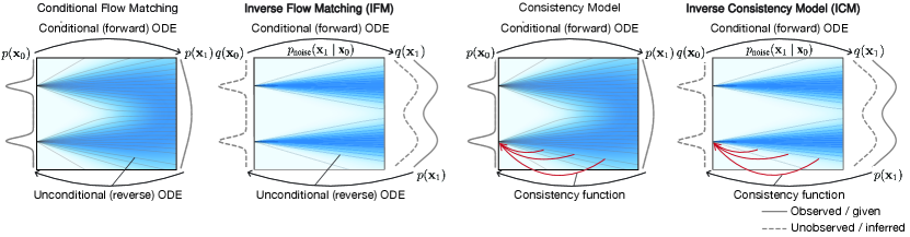
Recent advances in generative modeling such as diffusion models (Sohl-Dickstein et al., 2015; Ho et al., 2020; Song & Ermon, 2020; Song et al., 2021, 2022), conditional flow matching models (Lipman et al., 2023; Tong et al., 2024), and consistency models (Song et al., 2023; Song & Dhariwal, 2023) have achieved great success by learning a mapping from a simple prior distribution to the data distribution through an Ordinary Differential Equation (ODE) or Stochastic Differential Equation (SDE). We refer to their models as continuous-time generative models. These models typically involve defining a forward process, which transforms the data distribution to the prior distribution over time, and generation is achieved through learning a reverse process that can gradually transform the prior distribution to the data distribution (Figure 1).
Despite that those generative models are powerful tools for modeling the data distribution, they are not suitable for the inverse generation problems when the data distribution is not observed and only data transformed by a forward process is given, which is typically true for noisy real-world data measurements. Mapping from noisy data to the latent ground truth is especially important in various scientific applications when pushing the limit of measurement capabilities. This limitation necessitates the exploration of novel methodologies that can bridge the gap between generative modeling and effective denoising in the absence of clean data.
Here we propose a new approach called Inverse Flow (IF)111Code available at https://github.com/jzhoulab/InverseFlow, that learns a mapping from the observed noisy data distribution to the unobserved, ground truth data distribution (Figure 1), inverting the data requirement of generative models. An ODE or SDE is specified to reflect knowledge about the noise distribution. We further devised a pair of algorithms, Inverse Flow Matching (IFM) and Inverse Consistency Model (ICM) for learning inverse flows. Specifically, ICM involves a computationally efficient simulation-free objective that does not involve any ODE solver.
A main contribution of our approach is generalizing continuous-time generative models to inverse generation problems such as denoising without ground truth. In addition, in order to develop ICM, we generalized the consistency training objective for consistency models to any forward diffusion process or conditional flow. This broadens the scope of consistency model applications and has implications beyond denoising.
Compared to prior approaches for denoising without ground truth, IF offers the most flexibility in noise distribution, allowing almost any continuous noise distributions including those with complex dependency and transformations. IF can be seamlessly integrated with generative modeling to generate samples from the ground truth rather than the observed noisy distribution. More generally, IF models the past states of a (stochastic) dynamical system before the observed time points using the knowledge of its dynamics, which can have applications beyond denoising.
2 Background
2.1 Continuous-time generative models
Our proposed inverse flow framework is built upon continuous-time generative models such as diffusion models, conditional flow matching, and consistency models. Here we present a unified view of these methods that will help connect inverse flow with this entire family of models (Section 3).
These generative modeling methods are connected by their equivalence to continuous normalizing flow or neural ODE (Chen et al., 2019). They can all be considered as explicitly or implicitly learning the ODE that transforms between the prior distribution and the data distribution
| (1) |
in which represents the vector field of the ODE. We use the convention that corresponds to the data distribution and corresponds to the prior distribution. Generation is realized by reversing this ODE, which makes this family of methods a natural candidate for extension toward denoising problems.
Continuous-time generative models typically involve defining a conditional ODE or SDE that determines the that transforms the data distribution to the prior distribution. Training these models involves learning the unconditional ODE (Eq. 1) based on and the conditional ODE or SDE (Lipman et al., 2023; Tong et al., 2024; Song et al., 2021) (Figure 1). The unconditional ODE can be used for generation from noise to data.
2.1.1 Conditional flow matching
Conditional flow matching defines the transformation from data to prior distribution via a conditional ODE vector field . The unconditional ODE vector field is learned by minimizing the objective (Lipman et al., 2023; Tong et al., 2024; Albergo & Vanden-Eijnden, 2023):
| (2) |
where is sampled from the data distribution, and is sampled from the conditional distribution given by the conditional ODE.
The conditional ODE vector field can also be stochastically approximated through sampling from both prior distribution and data distribution and using the conditional vector field as the training target (Lipman et al., 2023; Tong et al., 2024):
| (3) |
This formulation has the benefit that can be easily chosen as any interpolation between and , because this interpolation does not affect the probability density at time 0 or 1 (Lipman et al., 2023; Tong et al., 2024; Albergo & Vanden-Eijnden, 2023; Albergo et al., 2023). For example, a linear interpolation corresponds to (Lipman et al., 2023; Tong et al., 2024; Liu et al., 2022). Sampling is realized by simulating the unconditional ODE with learned vector field in the reverse direction.
2.1.2 Consistency models
In contrast, consistency models (Song et al., 2023; Song & Dhariwal, 2023) learn consistency functions that can directly map a sample from the prior distribution to data distribution, equivalent to simulating the unconditional ODE in the reverse direction:
where denotes at time , and we use to denote simulating the ODE with vector field from time to time starting from . The consistency function is trained by minimizing the consistency loss (Song et al., 2023), which measures the difference between consistency function evaluations at two adjacent time points
| (4) | ||||
with the boundary condition . Stopgrad indicates that the term within the operator does not get optimized.
There are two approaches to training consistency models: one is distillation, and the other is training from scratch. In the consistency distillation objective, a pretrained diffusion model is used to obtain the unconditional ODE vector field , and and differs by one ODE step
| (5) | ||||
If the consistency model is trained from scratch, the consistency training objective samples and in a coupled manner from the forward diffusion process (Karras et al., 2022)
| (6) |
where controls the maximum noise level at . Consistency models have the advantage of fast generation speed as they can generate samples without solving any ODE or SDE.
2.1.3 Diffusion models
In diffusion models, the transformation from data to prior distribution is defined by a forward diffusion process (conditional SDE). The diffusion model training learns the score function which determines the unconditional ODE, also known as the probability flow ODE (Song et al., 2021).
Denoising applications of diffusion models
Diffusion models are inherently connected to denoising problems as the generation process is essentially a denoising process. However, existing denoising methods using diffusion models require training on ground truth data (Yue et al., 2023; Xie et al., 2023b), which is not available in inverse generation problems.
Ambient diffusion and GSURE-diffusion
Ambient Diffusion (Daras et al., 2023) and GSURE-diffusion (Kawar et al., 2024) address a related problem of learning the distribution of clean data by training on only linearly corrupted (linear transformation followed by additive Gaussian noise) data. Although those methods are designed for generation, they can be applied to denoising. Ambient Diffusion Posterior Sampling (Aali et al., 2024), further allowed using models trained with ambient diffusion on corrupted data to perform posterior sampling-based denoising for a different forward process (e.g., blurring). Consistent Diffusion Meets Tweedie (Daras et al., 2024) improves Ambient Diffusion by allowing exact sampling from clean data distribution using consistency loss with a double application of Tweedie’s formula. (Rozet et al., 2024) explored the potential of expectation maximization in training diffusion models on corrupted data. However, all these methods are restricted to training on linearly corrupted data, which still limit their applications when the available data is affected by other types of noises.
2.2 Denoising without ground truth
Denoising without access to ground truth data requires assumptions about the noise or the signal. Most contemporary approaches are based on assumptions about the noise, as the noise distribution is generally much simpler and better understood. Because prior methods have been comprehensively reviewed (Kim & Ye, 2021; Batson & Royer, 2019; Lehtinen et al., 2018; Xie et al., 2020; Soltanayev & Chun, 2018; Metzler et al., 2020), and our approach is not directly built upon these approaches, we only present a brief overview and refer the readers to Appendix LABEL:appendix:denoise referenced literature for more detailed discussion. None of these approaches are generally applicable to any noise types.
3 Inverse Flow and Consistency Models
In continuous-time generative models, usually the data from the distribution of interest is given. In contrast, in inverse generation problems, only the transformed data and the conditional distribution are given, whereas are unobserved. For example, are the noisy observations and is the conditional noise distribution. We define the Inverse Flow (IF) problem as finding a mapping from to which allows not only recovering the unobserved data distribution but also providing an estimate of from (Figure 1).
For denoising without ground truth applications, the inverse flow framework requires only the noisy data and the ability to sample from the noise distribution . This is thus applicable to any continuous noise and allows complex dependencies on the noise distribution, including noise that can only be sampled through a diffusion process.
Intuitively, without access to unobserved data , inverse flow algorithms train a continuous-time generative model using generated from observed data within the training loop (Figure 1). We demonstrated that this approach effectively recovers the unobserved distribution and learns a mapping from to .
3.1 Inverse Flow Matching
To solve the inverse flow problem, we first consider learning a mapping from to through an ODE with vector field . We propose to learn with the inverse flow matching (IFM) objective
| (7) | ||||
where the expectation is taken over , , and . This objective differs from conditional flow matching (Eq. 2) in two key aspects: using only transformed data rather than unobserved data , and choosing the conditional ODE based on the conditional distribution . Specifically,
-
1.
Sampling from the data distribution is replaced with sampling from and simulating the unconditional ODE backward in time based on the vector field , denoted as . We refer to this distribution as the recovered data distribution .
-
2.
The conditional ODE vector field is chosen to match the given conditional distribution at time .
For easier and more flexible application of IFM, similar to conditional flow matching (Eq. 3), an alternative form of the conditional ODE can be used instead of . Since is sampled from the noise distribution , the above condition is automatically satisfied. The conditional ODE vector field can be easily chosen as any smooth interpolation between and , such as . We detailed the inverse flow matching training in Algorithm 1 with the alternative form in Appendix A.1.
Next, we discuss the theoretical justifications of the IFM objective and the interpretation of the learned model. We show below that when the loss converges, the recovered data distribution matches the ground truth distribution . The proof is provided in Appendix LABEL:appendix:IFM.
Theorem 1
Assume that the noise distribution satisfies the condition that, for any noisy data distribution there exists only one probability distribution that satisfies , then under the condition that , we have the recovered data distribution .
Moreover, we show that with IFM the learned ODE trajectory from to can be intuitively interpreted as always pointing toward the direction of the estimated . More formally, the learned unconditional ODE vector field can be interpreted as an expectation of the conditional ODE vector field.
Lemma 1
Given a conditional ODE vector field that generates a conditional probability path , the unconditional probability path can be generated by the unconditional ODE vector field , which is defined as
| (8) |
The proof is provided in Appendix LABEL:appendix:IFM. Specifically, with the choice of , Eq. 8 has an intuitively interpretable form
| (9) |
which means that the unconditional ODE vector field at any time points straight toward the expected ground truth .
3.2 Simulation-free Inverse Flow with Inverse Consistency Model
IFM can be computationally expensive during training and inference because it requires solving ODE in each update. We address this limitation by introducing inverse consistency model (ICM), which learns a consistency function to directly solve the inverse flow without involving an ODE solver.
However, the original consistency training formulation is specific to one type of diffusion process (Karras et al., 2022), which is only applicable to independent Gaussian noise distribution for inverse generation application. Thus, to derive inverse consistency model that is applicable to any transformation, we first generalize consistency training so that it can be applied to arbitrary transformations and thus flexible to model almost any noise distribution.
3.2.1 Generalized Consistency Training
To recall from Section 2.1.2, consistency distillation is only applicable to distilling a pretrained diffusion or conditional flow matching model. The consistency training objective allows training consistency models from scratch but only for a specific forward diffusion process, which limits its flexibility in applying to any inverse generation problem.
Here we introduce generalized consistency training (GCT), which extends consistency training to any conditional ODE or forward diffusion process (through the corresponding conditional ODE). Intuitively, generalized consistency training modified consistency distillation (Eq. 4 and Eq. 5) in the same manner as how conditional flow matching modified the flow matching objective: instead of requiring the unconditional ODE vector field which is not available without a pretrained diffusion or conditional flow matching model, GCT only requires the user-specified conditional ODE vector field .
| (10) | ||||
Where the expectation is taken over , , and . An alternative formulation where the conditional flow is defined by is detailed in Appendix A.1.
We proved that the generalized consistency training (GCT) objective is equivalent to the consistency distillation (CD) objective (Eq. 4, Eq. 5). The proof is provided in Appendix LABEL:appendix:gct.
Theorem 2
Assuming the consistency function is twice differentiable with bounded second derivatives, and , up to a constant independent of , and are equal.
3.2.2 Inverse Consistency Models
With generalized consistency training, we can now provide the inverse consistency model (ICM) (Figure 1, Algorithm 2):
| (11) | ||||
which is the consistency model counterpart of IFM (Eq. 7). The expectation is taken over , , . Similar to IFM, a convenient alternative form is provided in Appendix A.1.
Since learning a consistency model is equivalent to learning a conditional flow matching model, ICM is equivalent to IFM following directly from our Theorem 2 and Theorem 1 from (Song et al., 2023).
Lemma 2
Assuming the consistency function is twice differentiable and is almost everywhere nonzero222 is required to ensure the existence of corresponding ODE, and it excludes trivial solution such as . With identity initialization of , we do not find it to be necessary for enforcing this condition in practice., when the inverse consistency loss , there exists a corresponding ODE vector field that minimized the inverse flow matching loss to .
The proof is provided in Appendix LABEL:appendix:lemma2. As in IFM, when the loss converges, the data distribution recovered by ICM matches the ground truth distribution , but ICM is much more computationally efficient as it is a simulation-free objective.
4 Experiments
We first demonstrated the performance and properties of IFM and ICM on synthetic inverse generation datasets, which include a deterministic problem of inverting Naiver-Stokes simulation and a stochastic problem of denoising a synthetic noise dataset 8-gaussians. Next, we demonstrated that our method outperforms prior methods (Mäkinen et al., 2020; Krull et al., 2019; Batson & Royer, 2019) with the same neural network architecture on a semi-synthetic dataset of natural images with three synthetic noise types, and a real-world dataset of fluorescence microscopy images. Finally, we demonstrated that our method can be applied to denoise single-cell genomics data.
4.1 Synthetic datasets
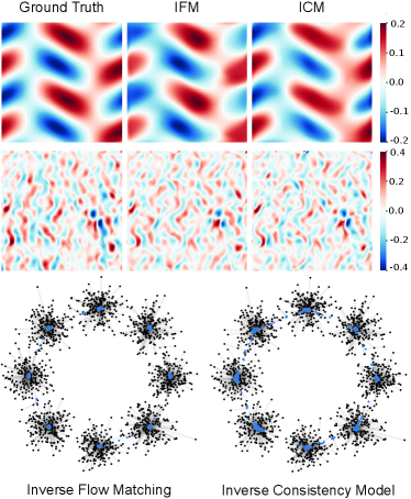
To test the capability of inverse flow in inverting complex transformations, we first attempted the deterministic inverse generation problem of inverting the transformation by Navier-Stokes fluid dynamics simulation333Inverse flow algorithms can be applied to deterministic transformations from to by using a matching conditional ODE, even though the general forms consider stochastic transforms described by .. We aim to recover the earlier state of the system without providing them for training (Figure 2). Navier-Stokes equations describe the motion of fluids by modeling the relationship between fluid velocity, pressure, viscosity, and external forces. These equations are fundamental in fluid dynamics and remain mathematically challenging, particularly in understanding turbulent flows. The details of the simulation are described in Appendix LABEL:appendix:syn_datasets.
To test inverse flow algorithms on a denoising inverse generation problem, we generated a synthetic 8-gaussians dataset (Appendix LABEL:appendix:syn_datasets for details). Both IFM and ICM are capable of noise removal (Figure 2). ICM achieved a similar denoising performance as IFM, even though it is much more computationally efficient due to the iterative evaluation of ODE (NFE=10) by IFM.
4.2 Semi-synthetic datasets
We evaluated the proposed method on images in the benchmark dataset BSDS500 (Arbeláez et al., 2011), Kodak, and Set12 (Zhang et al., 2017). To test the model’s capability to deal with various types of conditional noise distribution, we generated synthetic noisy images for three different types of noise, including correlated noise and adding noise through a diffusion process without a closed-form transition density function (Appendix LABEL:appendix:realdata for details). All models were trained using the BSDS500 training set and evaluated on the BSDS500 test set, Kodak, and Set12. We show additional qualitative results in Appendix LABEL:appendix:qualitative.
| Noise type | Input | Supervised | BM3D | Noise2Void | Noise2Self | Ours (ICM) | |
|---|---|---|---|---|---|---|---|
| Gaussian | BSDS500 | 20.17 | 28.00 | 27.49 | 26.54 | 27.79 | 28.16 |
| Kodak | 20.18 | 28.91 | 28.54 | 27.55 | 28.72 | 29.08 | |
| Set12 | 20.16 | 28.99 | 28.95 | 27.79 | 28.78 | 29.19 | |
| Correlated | BSDS500 | 20.17 | 27.10 | 24.48 | 26.32 | 21.03 | 27.64 |
| Kodak | 20.17 | 27.97 | 25.03 | 27.39 | 21.56 | 28.53 | |
| Set12 | 20.18 | 27.88 | 25.21 | 27.43 | 21.58 | 28.46 | |
| SDE (Jacobi process) | BSDS500 | 14.90 | 24.34 | 20.32 | 23.56 | 22.60 | 24.28 |
| Kodak | 14.76 | 25.34 | 20.42 | 23.99 | 23.70 | 25.07 | |
| Set12 | 14.80 | 25.01 | 20.51 | 24.43 | 23.26 | 24.74 | |
-
1.
Gaussian noise: we added independent Gaussian noise with fixed variance.
-
2.
Correlated noise: we employed convolution kernels to generate correlated Gaussian noise following the method in (Mäkinen et al., 2020)
(12) where and is a convolution kernel.
-
3.
Jacobi process: we transformed the data with Jacobi process (Wright-Fisher diffusion), as an example of SDE-based transform without closed-form conditional distribution
(13) We generated corresponding noise data by simulating the Jacobi process with and . Notably, the conditional noise distribution generated by the Jacobi process does not generally has an expectation that equals the ground truth (i.e. non-centered noise), which violates the assumptions of Noise2X methods.
Our approach outperformed alternative unsupervised methods in all three noise types, especially in correlated noise and Jacobi process (Appendix LABEL:appendix:qualitative, Table 1). This can be attributed to the fact that both Noise2X methods assumes independence of noise across different feature dimensions as well as centered-noise which were violated in corrleated noise and Jacobi process respectively.
Moreover, Our approach outperformed the supervised method on both Gaussian noise and correlated noise. Further analysis revealed that the supervised method encountered overfitting during the training process, which led to suboptimal performance. In contrast, our method did not exhibit such issues, highlighting the superiority of our approach.
In addition, in Appendix LABEL:appendix:addition, we conducted a series of experiments that demonstrate the reliability of our method under different intensities and types of noise. Furthermore, our method yielded satisfactory results even when there is a bias in the estimation of noise intensity. It also achieved excellent performance on RGB images and small sample-size datasets.
4.3 Real-world datasets
4.3.1 Fluorescence Microscopy data (FMD)
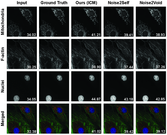
Fluorescence microscopy is an important scientific application of denoising without ground truth. Experimental constraints such as phototoxicity and frame rates often limit the capability to obtain clean data. We denoised confocal microscopy images from Fluorescence Microscopy Denoising (FMD) dataset (Zhang et al., 2019). We first fitted a signal-dependent Poisson-Gaussian noise model adopted from (Liu et al., 2013) for separate channels of each noisy microscopic images (Appendix LABEL:appendix:micro for details). Then denoising flow models were trained with the conditional ODE specified to be consistent with fitted noise model. Our method outperforms Noise2Self and Noise2Void, achieving superior denoising performance for mitochondria, F-actin, and nuclei in the microscopic images of BPAE cells (Figure 3).
4.3.2 Application to denoise single-cell genomics data
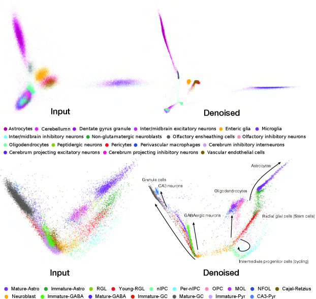
In recent years, the development of single-cell sequencing technologies has enabled researchers to obtain more fine-grained information on tissues and organs at the resolution of single cells. However, the low amount of sample materials per-cell introduces considerable noise in single-cell genomics data. These noises may obscure real biological signals, thereby affecting subsequent analyses.
Applying ICM to an adult mouse brain single-cell RNA-seq dataset (Zeisel et al., 2018) and a mouse brain development single-cell RNA-seq dataset (Hochgerner et al., 2018b) (Figure 4, Appendix LABEL:appendix:scRNA for details), we observed that the denoised data better reflects the cell types and developmental trajectories. We compared the original and denoised data by the accuracy of predicting the cell type identity of each cell based on its nearest neighbor in the top two principal components. Our methods improved the accuracy of the adult mouse brain dataset from to , and the mouse brain development dataset from to .
5 Limitation and Conclusion
We introduce Inverse Flow (IF), a generative modeling framework for inverse generation problems such as denoising without ground truth, and two methods Inverse Flow Match (IFM) and Inverse Consistency Model (ICM) to solve the inverse flow problem. Our framework connects the family of continuous-time generative models to inverse generation problems. Practically, we extended the applicability of denoising without ground truth to almost any continuous noise distributions. We demonstrated strong empirical results applying inverse flow. A limitation of inverse flow is assuming prior knowledge of the noise distribution, and future work is needed to relax this assumption. We expect inverse flow to open up possibilities to explore additional connections to the expanding family of continuous-time generative model methods, and the generalized consistency training objective will expand the application of consistency models.
References
- Aali et al. (2024) Asad Aali, Giannis Daras, Brett Levac, Sidharth Kumar, Alexandros G. Dimakis, and Jonathan I. Tamir. Ambient Diffusion Posterior Sampling: Solving Inverse Problems with Diffusion Models trained on Corrupted Data, March 2024. URL http://arxiv.org/abs/2403.08728. arXiv:2403.08728.
- Albergo & Vanden-Eijnden (2023) Michael S. Albergo and Eric Vanden-Eijnden. Building Normalizing Flows with Stochastic Interpolants, March 2023.
- Albergo et al. (2023) Michael S. Albergo, Nicholas M. Boffi, and Eric Vanden-Eijnden. Stochastic Interpolants: A Unifying Framework for Flows and Diffusions, November 2023.
- Arbeláez et al. (2011) Pablo Arbeláez, Michael Maire, Charless Fowlkes, and Jitendra Malik. Contour Detection and Hierarchical Image Segmentation. IEEE Transactions on Pattern Analysis and Machine Intelligence, 33(5):898–916, May 2011. ISSN 1939-3539. doi: 10.1109/TPAMI.2010.161.
- Avdeyev et al. (2023) Pavel Avdeyev, Chenlai Shi, Yuhao Tan, Kseniia Dudnyk, and Jian Zhou. Dirichlet Diffusion Score Model for Biological Sequence Generation, June 2023. URL http://arxiv.org/abs/2305.10699. arXiv:2305.10699 [cs, q-bio].
- Batson & Royer (2019) Joshua Batson and Loic Royer. Noise2Self: Blind Denoising by Self-Supervision, June 2019.
- Chen et al. (2019) Ricky T. Q. Chen, Yulia Rubanova, Jesse Bettencourt, and David Duvenaud. Neural Ordinary Differential Equations, December 2019.
- Daras et al. (2023) Giannis Daras, Kulin Shah, Yuval Dagan, Aravind Gollakota, Alexandros G. Dimakis, and Adam Klivans. Ambient Diffusion: Learning Clean Distributions from Corrupted Data, May 2023. URL http://arxiv.org/abs/2305.19256. arXiv:2305.19256 [cs, math].
- Daras et al. (2024) Giannis Daras, Alexandros G. Dimakis, and Constantinos Daskalakis. Consistent Diffusion Meets Tweedie: Training Exact Ambient Diffusion Models with Noisy Data, July 2024. URL http://arxiv.org/abs/2404.10177. arXiv:2404.10177.
- Ho et al. (2020) Jonathan Ho, Ajay Jain, and Pieter Abbeel. Denoising Diffusion Probabilistic Models, December 2020.
- Hochgerner et al. (2018a) Hannah Hochgerner, Amit Zeisel, Peter Lönnerberg, and Sten Linnarsson. Conserved properties of dentate gyrus neurogenesis across postnatal development revealed by single-cell RNA sequencing. Nature Neuroscience, 21(2):290–299, February 2018a. ISSN 1546-1726. doi: 10.1038/s41593-017-0056-2.
- Hochgerner et al. (2018b) Hannah Hochgerner, Amit Zeisel, Peter Lönnerberg, and Sten Linnarsson. Conserved properties of dentate gyrus neurogenesis across postnatal development revealed by single-cell RNA sequencing. Nature Neuroscience, 21(2):290–299, February 2018b. ISSN 1546-1726. doi: 10.1038/s41593-017-0056-2. URL https://www.nature.com/articles/s41593-017-0056-2. Publisher: Nature Publishing Group.
- Karras et al. (2022) Tero Karras, Miika Aittala, Timo Aila, and Samuli Laine. Elucidating the Design Space of Diffusion-Based Generative Models, October 2022.
- Kawar et al. (2024) Bahjat Kawar, Noam Elata, Tomer Michaeli, and Michael Elad. GSURE-Based Diffusion Model Training with Corrupted Data, June 2024. URL http://arxiv.org/abs/2305.13128. arXiv:2305.13128 [cs, eess].
- Kidger (2022) Patrick Kidger. On Neural Differential Equations, February 2022. URL http://arxiv.org/abs/2202.02435. arXiv:2202.02435 [cs].
- Kim & Ye (2021) Kwanyoung Kim and Jong Chul Ye. Noise2Score: Tweedie’s Approach to Self-Supervised Image Denoising without Clean Images, October 2021.
- Krull et al. (2019) Alexander Krull, Tim-Oliver Buchholz, and Florian Jug. Noise2Void - Learning Denoising from Single Noisy Images, April 2019. URL http://arxiv.org/abs/1811.10980. arXiv:1811.10980 [cs].
- Lehtinen et al. (2018) Jaakko Lehtinen, Jacob Munkberg, Jon Hasselgren, Samuli Laine, Tero Karras, Miika Aittala, and Timo Aila. Noise2Noise: Learning Image Restoration without Clean Data, October 2018.
- Lipman et al. (2023) Yaron Lipman, Ricky T. Q. Chen, Heli Ben-Hamu, Maximilian Nickel, and Matt Le. Flow Matching for Generative Modeling, February 2023.
- Liu et al. (2022) Xingchao Liu, Chengyue Gong, and Qiang Liu. Flow Straight and Fast: Learning to Generate and Transfer Data with Rectified Flow, September 2022.
- Liu et al. (2013) Xinhao Liu, Masayuki Tanaka, and Masatoshi Okutomi. Estimation of signal dependent noise parameters from a single image. In 2013 IEEE International Conference on Image Processing, pp. 79–82, September 2013. doi: 10.1109/ICIP.2013.6738017. URL https://ieeexplore.ieee.org/document/6738017. ISSN: 2381-8549.
- Loshchilov & Hutter (2019) Ilya Loshchilov and Frank Hutter. Decoupled Weight Decay Regularization, January 2019.
- Mäkinen et al. (2020) Ymir Mäkinen, Lucio Azzari, and Alessandro Foi. Collaborative Filtering of Correlated Noise: Exact Transform-Domain Variance for Improved Shrinkage and Patch Matching. IEEE Transactions on Image Processing, 29:8339–8354, 2020. ISSN 1941-0042. doi: 10.1109/TIP.2020.3014721.
- Metzler et al. (2020) Christopher A. Metzler, Ali Mousavi, Reinhard Heckel, and Richard G. Baraniuk. Unsupervised Learning with Stein’s Unbiased Risk Estimator, July 2020.
- Mohan et al. (2021) Sreyas Mohan, Ramon Manzorro, Joshua L. Vincent, Binh Tang, Dev Yashpal Sheth, Eero P. Simoncelli, David S. Matteson, Peter A. Crozier, and Carlos Fernandez-Granda. Deep Denoising For Scientific Discovery: A Case Study In Electron Microscopy, July 2021. URL http://arxiv.org/abs/2010.12970. arXiv:2010.12970.
- Paszke et al. (2019) Adam Paszke, Sam Gross, Francisco Massa, Adam Lerer, James Bradbury, Gregory Chanan, Trevor Killeen, Zeming Lin, Natalia Gimelshein, Luca Antiga, Alban Desmaison, Andreas Köpf, Edward Yang, Zach DeVito, Martin Raison, Alykhan Tejani, Sasank Chilamkurthy, Benoit Steiner, Lu Fang, Junjie Bai, and Soumith Chintala. PyTorch: An Imperative Style, High-Performance Deep Learning Library, December 2019.
- Rozet et al. (2024) François Rozet, Gérôme Andry, François Lanusse, and Gilles Louppe. Learning Diffusion Priors from Observations by Expectation Maximization, November 2024. URL http://arxiv.org/abs/2405.13712. arXiv:2405.13712.
- Sohl-Dickstein et al. (2015) Jascha Sohl-Dickstein, Eric Weiss, Niru Maheswaranathan, and Surya Ganguli. Deep Unsupervised Learning using Nonequilibrium Thermodynamics. In Proceedings of the 32nd International Conference on Machine Learning, pp. 2256–2265. PMLR, June 2015.
- Soltanayev & Chun (2018) Shakarim Soltanayev and Se Young Chun. Training deep learning based denoisers without ground truth data. In Advances in Neural Information Processing Systems, volume 31. Curran Associates, Inc., 2018.
- Song et al. (2022) Jiaming Song, Chenlin Meng, and Stefano Ermon. Denoising Diffusion Implicit Models, October 2022.
- Song & Dhariwal (2023) Yang Song and Prafulla Dhariwal. Improved Techniques for Training Consistency Models, October 2023.
- Song & Ermon (2020) Yang Song and Stefano Ermon. Generative Modeling by Estimating Gradients of the Data Distribution, October 2020.
- Song et al. (2021) Yang Song, Jascha Sohl-Dickstein, Diederik P. Kingma, Abhishek Kumar, Stefano Ermon, and Ben Poole. Score-Based Generative Modeling through Stochastic Differential Equations, February 2021.
- Song et al. (2023) Yang Song, Prafulla Dhariwal, Mark Chen, and Ilya Sutskever. Consistency Models, May 2023.
- Spalart et al. (1991) Philippe R Spalart, Robert D Moser, and Michael M Rogers. Spectral methods for the Navier-Stokes equations with one infinite and two periodic directions. Journal of Computational Physics, 96(2):297–324, October 1991. ISSN 0021-9991. doi: 10.1016/0021-9991(91)90238-G. URL https://www.sciencedirect.com/science/article/pii/002199919190238G.
- Tong et al. (2024) Alexander Tong, Kilian Fatras, Nikolay Malkin, Guillaume Huguet, Yanlei Zhang, Jarrid Rector-Brooks, Guy Wolf, and Yoshua Bengio. Improving and generalizing flow-based generative models with minibatch optimal transport, March 2024.
- Wolf et al. (2018) F. Alexander Wolf, Philipp Angerer, and Fabian J. Theis. SCANPY: Large-scale single-cell gene expression data analysis. Genome Biology, 19(1):15, February 2018. ISSN 1474-760X. doi: 10.1186/s13059-017-1382-0.
- Xie et al. (2020) Yaochen Xie, Zhengyang Wang, and Shuiwang Ji. Noise2Same: Optimizing A Self-Supervised Bound for Image Denoising, October 2020.
- Xie et al. (2023a) Yutong Xie, Mingze Yuan, Bin Dong, and Quanzheng Li. Unsupervised Image Denoising with Score Function, April 2023a. URL http://arxiv.org/abs/2304.08384. arXiv:2304.08384.
- Xie et al. (2023b) Yutong Xie, Minne Yuan, Bin Dong, and Quanzheng Li. Diffusion Model for Generative Image Denoising, February 2023b. URL http://arxiv.org/abs/2302.02398. arXiv:2302.02398 [cs].
- Yue et al. (2023) Zongsheng Yue, Jianyi Wang, and Chen Change Loy. ResShift: Efficient Diffusion Model for Image Super-resolution by Residual Shifting, October 2023. URL http://arxiv.org/abs/2307.12348. arXiv:2307.12348 [cs].
- Zeisel et al. (2018) Amit Zeisel, Hannah Hochgerner, Peter Lönnerberg, Anna Johnsson, Fatima Memic, Job van der Zwan, Martin Häring, Emelie Braun, Lars E. Borm, Gioele La Manno, Simone Codeluppi, Alessandro Furlan, Kawai Lee, Nathan Skene, Kenneth D. Harris, Jens Hjerling-Leffler, Ernest Arenas, Patrik Ernfors, Ulrika Marklund, and Sten Linnarsson. Molecular Architecture of the Mouse Nervous System. Cell, 174(4):999–1014.e22, August 2018. ISSN 0092-8674. doi: 10.1016/j.cell.2018.06.021. URL https://www.sciencedirect.com/science/article/pii/S009286741830789X.
- Zhang et al. (2017) Kai Zhang, Wangmeng Zuo, Yunjin Chen, Deyu Meng, and Lei Zhang. Beyond a Gaussian Denoiser: Residual Learning of Deep CNN for Image Denoising. IEEE Transactions on Image Processing, 26(7):3142–3155, July 2017. ISSN 1941-0042. doi: 10.1109/TIP.2017.2662206.
- Zhang et al. (2019) Yide Zhang, Yinhao Zhu, Evan Nichols, Qingfei Wang, Siyuan Zhang, Cody Smith, and Scott Howard. A Poisson-Gaussian Denoising Dataset with Real Fluorescence Microscopy Images, April 2019. URL http://arxiv.org/abs/1812.10366. arXiv:1812.10366 [cs, eess, stat].
Appendix A Appendix
A.1 Alternative forms of IFM and ICM
Here we provide the details of alternative objectives and corresponding algorithms of IFM and ICM which are easier and flexible to use.
A.1.1 Alternative objectives of IFM and ICM
We define the alternative objective of IFM similar to conditional flow matching (Eq. 3):
| (14) |
where is sampled from the conditional noise distribution. As described in Section 2.1.1 can be easily chosen as any smooth interpolation between and , such as .
Since ICM is based on generalized consistency training, we first provide the alternative objective of generalized consistency training
| (15) | |||
where the conditional flow is defined jointly by and .
Then the alterntive form of ICM can be defined as
| (16) | ||||
where can be freely defined based on any interpolation between and , which is more easily applicable to any conditional noise distribution:.