Inverse Scattering Method Solves the Problem of Full Statistics of Nonstationary Heat Transfer in the Kipnis-Marchioro-Presutti Model

Introduction. – Full statistics of currents of matter or energy in macroscopic systems away from thermodynamic equilibrium is a fundamental quantity that has attracted much attention from statistical physicists in the past two decades. Major progress has been achieved in determining this quantity for nonequilibrium steady states in simple models of interacting particles Derrida2007 ; BlytheEvans ; AppertRolland ; Lecomte . Nonstationary fluctuations of current, however, proved to be much harder for analysis DG2009a ; DG2009b ; KrMe ; MS2013 ; MS2014 ; VMS2014 ; ZarfatyM .

A convenient and widely used family of models for studying the full statistics of currents is stochastic lattice gases Spohn ; Liggett ; KL ; Krapivskybook . One important example is the Kipnis-Marchioro-Presutti (KMP) model of heat transfer. The KMP model involves immobile particles occupying a whole lattice and carrying continuous amounts of energy. At each random move the total energy of a randomly chosen pair of nearest neighbors is randomly redistributed among them according to uniform distribution. The KMP model originally attracted much interest as the first model for which Fourier’s law of heat diffusion at a coarse-grained level was proven rigorously KMP . By now it has become a paradigmatic model of nonequilibrium fluctuations of transport Bertini2005 ; BGL ; BodineauDerrida ; DG2009b ; Lecomte ; Tailleur ; HurtadoGarrido ; KrMe ; Pradosetal ; MS2013 ; Peletier ; ZarfatyM ; Spielberg ; Guttierez ; Frassek ; Benichou .

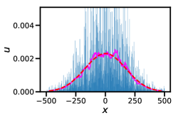
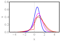
Here we study a full non-stationary heat-transfer statistics in the KMP model on an infinite one-dimensional lattice. Suppose that only one particle has a nonzero energy at $t=0$. Due to the energy exchange with the neighbors, the energy will start spreading throughout the system. At times much longer than the inverse rate of the energy exchange between the two neighbors (equal to $1/2$), and at distances much larger than the lattice constant (equal to $1$), the mean coarse-grained temperature $\bar{u}(x,t)$ in the KMP model is governed by the heat diffusion equation KMP ; Spohn ; KL $\partial_{t}\bar{u}(x,t)=\partial_{x}^{2}\bar{u}(x,t)$. The initial temperature is a delta-function, $\bar{u}(x,t=0)=W\delta(x)$, and so the solution is

$$\bar{u}(x,t)=(W/\sqrt{4\pi t})\,\exp(-x^{2}/4t)\,.$$

(1)

However, in stochastic realizations of the KMP model the coarse-grained temperature will fluctuate around the expected profile $\bar{u}(x,t)$, see Fig. 1. To characterize these non-stationary fluctuations, we will consider the total amount of heat $W_{>}$, observed on the right half line $x>0$ at time $t=T\gg 1$. The expected value of $W_{>}$ is $W/2$, and we will study the full time-dependent statistics of the heat excess, $J=\int_{0}^{\infty}u(x,t=T)\,dx-W/2$. Obviously $\mathcal{P}(J,T)$, the probability distribution of $J$ at time $T$, has a compact support $|J|\leq W/2$.

Similar non-stationary large-deviation settings, but with a step-like initial condition for the particle density or temperature, have been recently studied for a whole family of diffusive lattice gases DG2009b ; KrMe ; MS2013 ; MS2014 ; VMS2014 , of which the KMP model is an important particular case. The main working tool of these studies has been the macroscopic fluctuation theory (MFT) JonaLasinioreview : a weak-noise theory, whose starting point is fluctuational hydrodynamics (FH) Spohn ; KL ; LL . The FH is a coarse-grained description of the lattice gas, which is accurate when the characteristic length scale of the problem (here the diffusion length $\sqrt{T}$) and the observation time $T$ are much larger than the lattice constant $1$ and the inverse elemental rate $1/2$ of the energy exchange, respectively. For diffusive lattice gases with a single conservation law the FH has the form of a single macroscopic Langevin equation, which accounts for the fluctuational contribution to the heat or mass flux. For the KMP model the Langevin equation reads Spohn ; KL

$$\partial_{t}u=\partial_{x}\left(\partial_{x}u+\sqrt{2}u\eta\right)\,,$$

(2)

where $u(x,t)$ is the temperature, and $\eta(x,t)$ is a delta-correlated Gaussian noise: $\left<\eta(x,t)\right>=0$ and $\quad\left<\eta(x,t)\eta(x^{\prime},t^{\prime})\right>=\delta(x-x^{\prime})\delta(t-t^{\prime})$.

The MFT JonaLasinioreview relies on a saddle-point evaluation of the path integral for the stochastic process, described by Eq. (2). The small parameter of the saddle-point evaluation is again $1/\sqrt{T}\ll 1$: long times correspond to a weak noise. The saddle-point evaluation of the path integral boils down to a minimization of the action functional SM , constrained by the specified heat excess $J$ at $t=T$ and obeying the specified initial condition $u(x,t=0)$. For the statistics of the heat (or mass) excess, the MFT equations and boundary conditions in time were derived in Ref. DG2009b , and we will present them shortly. For completeness, we also present their derivation in SM . The solution of the MFT problem describes the optimal path of the process: the most likely time history of the temperature field $u(x,t)$ which dominates the probability distribution $\mathcal{P}(J,T)$ that we are after. The MFT problem, however, has proven to be very hard to solve analytically, especially for quenched (that is, deterministic) initial conditions annealed . In particular, for the KMP model, only small-$J$ KrMe and large-$J$ MS2013 asymptotes have been obtained until now (but for a step-like initial condition).

This Letter reports a major advance in this area of statistical mechanics. We present an exact solution to the heat excess statistics problem by uncovering and exploiting complete integrability of the underlying MFT equations. We obtain explicit results for an initially localized heat pulse, $u(x,t=0)=W\delta(x)$, for which we uncover a nontrivial time-reversal mirror symmetry. These are the first exact non-steady-state large-deviation results for the statistics of current in a lattice gas of interacting particles for quenched initial conditions.

Formulation of the MFT problem DG2009b ; SM . – Let us rescale $t$, $x$ and $u$ by $T$, $\sqrt{T}$ and $W/\sqrt{T}$, respectively. The optimal path we are after is described by two coupled Hamilton’s equations for the rescaled temperature field $u(x,t)$ and the conjugate “momentum density” field $p(x,t)$ which describes the optimal history of the noise $\eta(x,t)$, conditioned on the heat excess $J$.

It is convenient to introduce the (minus) gradient field $v(x,t)=-\partial_{x}p(x,t)$. In the variables $u$ and $v,$ the MFT equations take the form DG2009b ; MS2013 ; SM

	$\displaystyle\partial_{t}u$	$\displaystyle=$	$\displaystyle\partial_{x}(\partial_{x}u+2u^{2}v)\,,$		(3)
	$\displaystyle\partial_{t}v$	$\displaystyle=$	$\displaystyle\partial_{x}(-\partial_{x}v+2uv^{2})\,.$		(4)

The rescaled initial condition is

$$u(x,t=0)=\delta(x)\,.$$

(5)

The condition on the heat excess at $t=T$ becomes

$$\int_{0}^{\infty}u(x,t=1)\,dx-\frac{1}{2}=j\equiv\frac{J}{W}\,.$$

(6)

The minimization of the action functional, that enters the constrained path integral, with respect to variations of $u(x,t)$ yields, aside from Eqs. (3) and (4), a second boundary condition in time DG2009b ,

$$v(x,t=1)=-\lambda\,\delta(x)\,,$$

(7)

where $\lambda$ plays the role of a Lagrange multiplier, to be ultimately fixed by the constraint (6).

Once $u(x,t)$ and $v(x,t)$ are found, one can calculate the rescaled action, which can be written as DG2009b ; KrMe ; MS2013

$\displaystyle s=\int_{0}^{1}dt\int_{-\infty}^{\infty}dx\,u^{2}v^{2}.$

(8)

The action yields the probability density ${\cal P}(J,T,W)$ up to a pre-exponent:

$$\ln{\mathcal{P}}(J,T,W)\simeq-\sqrt{T}\,s\left(\frac{J}{W}\right).$$

(9)

Since $\sqrt{T}\gg 1$, Eq. (9) has a clear large-deviation structure, and the action $s$ plays the role of a rate function.

A crucial and previously unappreciated observation is that Eqs. (3) and (4) coincides with the derivative nonlinear Schrödinger (DNLS) equation in imaginary time and space DNLSE . The DNLS equation (with real time and space) describes propagation of nonlinear electromagnetic waves in plasmas and other media KN . An initial-value problem for the DNLS equation is completely integrable via the Zakharov-Shabat inverse scattering method (ISM) adapted by Kaup and Newell for the DNLS KN . The MFT formulation presents an difficulty, however, as here one needs to solve a boundary-value problem in time, rather than an initial-value problem. Here we overcome this difficulty by (i) making use of a shortcut that allows one to determine the rate function $s(j)$ even without the knowledge of $u(x,t)$ and $v(x,t)$ for all $t$, and (ii) exploiting a previously unknown symmetry relation symmetry , specific to the initial condition (5):

$$v(x,t)=-\lambda\,u(-x,1-t)\,.$$

(10)

Solution of the MFT problem.– Equations (3) and (4) belong to a class of integrable systems for which a Lax pair exists, i.e., as we explain below, the equations are equivalent to the compatibility condition of a system of two linear differential equations. The latter system defines scattering amplitudes which depend on $u$ and $v$. The idea behind the approach that we shall use – the ISM – is to consider the time evolution of these scattering amplitudes, which turns out to be very simple, as shown below. By relating these scattering amplitudes, at $t=0$ and $t=1$, to the fields $u$ and $v$, the method will enable us to find the heat excess $j=j(\lambda)$ which suffices for the calculation of $s=s(j)$.

Adapting the derivation of Kaup and Newell KN to imaginary time and space, we consider the linear system

$$\begin{cases}\partial_{x}\mathbold{\psi}(x,t,k)=U(x,t,k)\mathbold{\psi}(x,t,k)\,,\\ \partial_{t}\mathbold{\psi}(x,t,k)=V(x,t,k)\mathbold{\psi}(x,t,k)\,,\end{cases}$$

(11)

where $\mathbold{\psi}(x,t,k)$ is a column vector of dimension 2,

$$U(x,t,k)=\begin{pmatrix}-ik/2&-iv\sqrt{ik}\\ -iu\sqrt{ik}&ik/2\\ \end{pmatrix},\;V(x,t,k)=\begin{pmatrix}k^{2}/2-ikuv&-i(\sqrt{ik})^{3}v+i\sqrt{ik}\,\partial_{x}v-i\sqrt{ik}2v^{2}u\\ -i(\sqrt{ik})^{3}u+i\sqrt{ik}\,\partial_{x}u-i\sqrt{ik}2u^{2}v&-k^{2}/2+ikuv,\\ \end{pmatrix},$$

(12)

and $k$ is a spectral parameter. As one can check, the compatibility condition $\partial_{t}\partial_{x}\mathbold{\psi}=\partial_{x}\partial_{t}\mathbold{\psi}$, which corresponds to

$$\partial_{t}U-\partial_{x}V+\left[U,V\right]=0,$$

(13)

is indeed equivalent to Eqs. (3) and (4).

Let us define the matrix $\mathcal{T}(x,y,t,k)$ as the $x$-propagator of the system (11), namely, the solution to

$$\partial_{x}\mathcal{T}(x,y,t,k)=U(x,t,k)\mathcal{T}(x,y,t,k)$$

(14)

with $\mathcal{T}(x,x,t,k)=I$ (the identity matrix). At $x\to\pm\infty$, where the fields $u(x,t)$ and $v(x,t)$ vanish, the matrix $U$ becomes very simple,

$$U(x\to\pm\infty,t,k)=\begin{pmatrix}-ik/2&0\\ 0&ik/2\end{pmatrix}\,.$$

(15)

Therefore, it is natural to define the full-space propagator $G(t,k)$ as follows:

	$\displaystyle G(t,k)$	$\displaystyle=\lim_{\begin{array}[]{c}x\to\infty\\ y\to-\infty\end{array}}\begin{pmatrix}e^{ikx/2}&0\\ 0&e^{-ikx/2}\end{pmatrix}$		(18)
		$\displaystyle\times\mathcal{T}(x,y,t,k)\begin{pmatrix}e^{-iky/2}&0\\ 0&e^{iky/2}\end{pmatrix}.$		(19)

The entries of the matrix $G(t,k)$ are the scattering amplitudes of the system (11). The time evolution of $G(t,k)$ is easy to find. Indeed, the matrix $\mathcal{T}(x,y,t,k)$ satisfies:

	$\displaystyle\partial_{t}\mathcal{T}(x,y,t,k)$	$\displaystyle=$	$\displaystyle V(x,t,k)\mathcal{T}(x,y,t,k)$		(20)
		$\displaystyle-$	$\displaystyle\mathcal{T}(x,y,t,k)V(y,t,k).$

One can check that Eq. (20) is compatible with (14) (i.e. $\partial_{t}\partial_{x}\mathcal{T}=\partial_{x}\partial_{t}\mathcal{T}$) due to Eq. (13). The matrix $V(x,t,k)$ too becomes very simple in the limit $x\to\pm\infty$,

$$V(x\to\pm\infty,t,k)=\frac{k^{2}}{2}\begin{pmatrix}1&0\\ 0&-1\end{pmatrix}\,.$$

(21)

Plugging (21) into (20), one finds the time evolution of $\mathcal{T}(x\to\infty,y\to-\infty,t,k)$ which in turn, using (18), yields that of $G(t,k):$

$\displaystyle G(t,k)=\begin{pmatrix}a(t,k)&\tilde{b}(t,k)\\ b(t,k)&\tilde{a}(t,k)\\ \end{pmatrix}=\begin{pmatrix}a(0,k)&\tilde{b}(0,k)e^{k^{2}t}\\ b(0,k)e^{-k^{2}t}&\tilde{a}(0,k)\\ \end{pmatrix}$

(22)

where we have introduced here a notation for the matrix elements of $G(t,k)$.

Plugging the temporal boundary conditions (5) and (7), we calculate $G(0,k)$ and $G(1,k)$ explicitly by solving Eq. (14), see SM . Comparing the two solutions and using (22) we obtain

$$ik\left[Q_{+}(k)+Q_{-}(k)\right]-ikQ_{-}(k)\times ikQ_{+}(k)=-\lambda ike^{-k^{2}}$$

(23)

where $Q_{\pm}(k)$ are the Fourier transforms of $v(z,0)$ restricted to $z>0$ and $z<0$, respectively:

$$Q_{-}(k)\!=\!\int_{-\infty}^{0}\!v(z,0)e^{ikz}dz,\;\;Q_{+}(k)=\int_{0}^{\infty}\!v(z,0)e^{ikz}dz\,.$$

(24)

We solve Eq. (23) in SM , with the result

	$\displaystyle ikQ_{\pm}(k)$	$\displaystyle=1-\left(1\pm v_{\pm}\right)e^{\Phi_{\pm}\left(k\right)},$		(25)
	$\displaystyle\Phi_{\pm}\left(k\right)$	$\displaystyle=\pm\int_{-\infty}^{\infty}\frac{\ln\left(1+i\lambda k^{\prime}e^{-k^{\prime 2}}\right)}{k^{\prime}-k\mp i0^{+}}\frac{dk^{\prime}}{2\pi i}\,,$		(26)

where $v_{\pm}=v(0^{\pm},0)$.

To compute $v_{\pm},$ we demand that $Q_{\pm}(k)$ be regular at the origin, corresponding to a vanishing $v(z,0)$ at infinity. Setting $k=0$ in Eq. (25) and using the Sokhotski–Plemelj formula

$$\int_{-\infty}^{\infty}\frac{f(k)}{k\pm i0^{+}}\frac{dk}{2\pi i}=\mathchoice{{\vbox{\hbox{$\textstyle-$}}\kern-4.86108pt}}{{\vbox{\hbox{$\scriptstyle-$}}\kern-3.25pt}}{{\vbox{\hbox{$\scriptscriptstyle-$}}\kern-2.29166pt}}{{\vbox{\hbox{$\scriptscriptstyle-$}}\kern-1.875pt}}\!\int_{-\infty}^{\infty}\frac{f(k)}{k}\frac{dk}{2\pi i}\mp\frac{1}{2}f(0)\,,$$

(27)

we obtain after some algebra

$\displaystyle\pm v_{\pm}=\exp\left[\mp\int_{-\infty}^{\infty}\text{arctan}\left(\lambda k^{\prime}e^{-k^{\prime 2}}\right)\frac{dk^{\prime}}{2\pi k^{\prime}}\right]-1\,.$

(28)

Taking the derivative of Eq. (25) with respect to $k$ at $k=0$, yields SM

$$Q_{+}(0)=\frac{1}{4\pi}\int_{-\infty}^{\infty}\frac{\ln\left(1+\lambda^{2}k^{2}e^{-2k^{2}}\right)}{k^{2}}\,dk\,-\frac{\lambda}{2}\,.$$

(29)

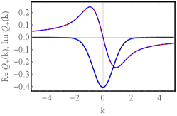
Figure 2 shows $\text{Re}\,Q_{+}(k)$ and $\text{Im}\,Q_{+}(k)$ versus $k$ at $\lambda=1$, obtained by plugging Eq. (28) for $v_{\pm}$ into Eq. (25). This figure also shows the same quantities computed by solving Eqs. (3) and (4) numerically with a back-and-forth iteration algorithm CS . The analytical and numerical curves are almost indistinguishable.

Using Eqs. (6), (10) and (24) alongside with the conservation law $\int_{-\infty}^{\infty}u(x,t)\,dx=1$, we determine $j=j(\lambda)$:

$$j\left(\lambda\right)=\frac{Q_{+}\left(0\right)}{\lambda}+\frac{1}{2}=\frac{1}{4\pi\lambda}\int_{-\infty}^{\infty}\frac{\ln\left(1+\lambda^{2}k^{2}e^{-2k^{2}}\right)}{k^{2}}\,dk\,.$$

(30)

Now we use a shortcut which makes the results we have obtained so far sufficient for obtaining the rate function $s=s(j)$. The shortcut comes in the form of the relation $ds/dj=\lambda$, which follows from the fact that $j$ and $\lambda$ are conjugate variables, see e.g. Ref. Vivoetal . It allows one to calculate $s(j)$ bypassing Eq. (8) [which would require the knowledge of the whole optimal path $u(x,t)$]. We have

$$\frac{ds}{d\lambda}=\frac{ds}{dj}\frac{dj}{d\lambda}=\lambda\frac{dj}{d\lambda}=\frac{dQ_{+}\left(0\right)}{d\lambda}-\frac{Q_{+}\left(0\right)}{\lambda}\,.$$

(31)

Using Eq. (29), we integrate Eq. (31) with respect to $\lambda$ to get

$$s(\lambda)=Q_{+}(0)+\int_{-\infty}^{\infty}\frac{\text{Li}_{2}\left(-\lambda^{2}k^{2}e^{-2k^{2}}\right)}{8\pi k^{2}}\,dk\,+\frac{\lambda}{2}.$$

(32)

where $\text{Li}_{2}\left(z\right)=\sum_{k=1}^{\infty}z^{k}/k^{2}$ is the dilogarithm function, $Q_{+}(0)$ is given by Eq. (29), and the integration constant was determined from $s(\lambda=0)=0$. Equations (30) and (32) give the complete rate function $s(j)$ in a parametric form and represent the main result of this work. The exact optimal history of the temperature profile $u(x,t)$ proved difficult to obtain analytically, but it can be computed numerically SM .

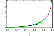
Figure 3 shows $s(j)$ alongside with two asymptotes: $j\to 0$ and $|j|\to 1/2$, which correspond to $\lambda\to 0$ and $|\lambda|\to\infty$, respectively. Also shown are results of Monte-Carlo simulations. The asymptote $\lambda\to 0$ can be obtained either from the exact rate function (30) and (32) SM , or from a perturbative expansion applied directly to the MFT equations KrMe . By virtue of the symmetry (10), the latter can be done very easily. Indeed, in the leading order in $\lambda\ll 1$ Eqs. (8), (10) and (1) yield

$$s(\lambda)\!\simeq\!\lambda^{2}\!\int_{0}^{1}\!dt\int_{-\infty}^{\infty}\!dx\,\bar{u}^{2}(x,t)\,\bar{u}^{2}(-x,1-t)=\frac{\lambda^{2}}{8\sqrt{2\pi}}\,.$$

(33)

The shortcut relation $ds/dj=\lambda$ can be rewritten as $(ds/d\lambda)(d\lambda/dj)=\lambda$. Combined with Eq. (33) it yields $s(j\to 0)\simeq\sqrt{8\pi}j^{2}$. Then, from Eq. (9), we see that typical fluctuations of $J$ are normally distributed with variance $W^{2}/(32\pi T)^{1/2}$. The $T^{-1/2}$ scaling of the variance should be contrasted with the $T^{1/2}$ scaling, obtained for a step-like initial condition DG2009b ; DG2009a ; KrMe . However, the relative magnitude of the fluctuations – the ratio of the standard deviation and the average transferred heat – has the same scaling $T^{-1/4}\ll 1$ in both settings, as to be expected from the law of large numbers.

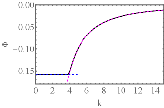
The asymptote of $|\lambda|\to\infty$ is more subtle SM . The final result, already in terms of $j$, is

		$\displaystyle s\left(|j|\to 1/2\right)\simeq\frac{4\left[-\frac{1}{2}W_{-1}\left(-\frac{1}{2}\pi^{2}\Delta^{2}\right)\right]^{3/2}}{3\pi}$
		$\displaystyle=\frac{4}{3\pi}\ln^{3/2}\left(\frac{2}{\pi\Delta}\,\sqrt{\ln\frac{2}{\pi\Delta}\sqrt{\ln\frac{2}{\pi\Delta}\dots}}\right)\,,$		(34)

where $\Delta\equiv 1/2-|j|\ll 1$, and $W_{-1}(\dots)$ is the proper branch of the product log (Lambert $W$) function LambertW . At $j=1/2$, $s$ diverges and $\mathcal{P}$ vanishes, as to be expected. Nested-log large-current asymptotes similar to Eq. (Inverse Scattering Method Solves the Problem of Full Statistics of Nonstationary Heat Transfer in the Kipnis-Marchioro-Presutti Model) appear to be typical for the KMP model and other models of the hyperbolic universality class MS2013 ; MS2014 ; ZarfatyM .

Discussion.– By combining the MFT and the ISM, we calculated exactly the rate function $s(j)$, see Eqs. (30) and (32), which describes the full long-time statistics of nonstationary heat transfer in the KMP model for an initially localized heat pulse. This is the first exact non-steady-state large-deviation result for the statistics of current in a lattice gas of interacting particles for quenched initial conditions. It opens the way to extensions of the ISM to additional fluctuating quantities of the KMP model. Another challenging goal is to apply the ISM to the simple symmetric exclusion process (SSEP) Spohn ; Liggett ; KL ; Krapivskybook – a lattice-gas model with quite different properties MS2014 . Encouragingly, the MFT equations for the SSEP (see e.g. DG2009b ) can be mapped to Eqs. (3) and (4) via a canonical transformation. This transformation, however, complicates the boundary conditions in time.

From a more general perspective, the MFT of lattice gases is a particular case of the weak-noise theory, or optimal fluctuation method (OFM): a highly versatile framework which captures a broad class of large deviations in macroscopic systems. For non-stationary processes the OFM equations – coupled nonlinear partial differential equations for the optimal path – are usually very hard to solve exactly. One class of problems of this type, which has received much recent attention, deals with the complete one-point height statistics of an interface whose dynamics is described by the Kardar-Parisi-Zhang (KPZ) equation KPZ . The OFM captures the complete KPZ height statistics at short times KK ; MKV ; KMS ; JKM ; Lin ; Lamarre . Here too, a previous analytical progress in the solution of the OFM equations was limited to asymptotics of very large or very small interface height. But very recently these OFM equations – which coincide with the Nonlinear Schrödinger equation (NLS) (not the derivative one) JKM – have been solved exactly KLD1 ; KLD2 by the ISM for several “standard” initial conditions. The two integrable systems, the NLS and DNLS, are closely related, so our approach can be compared with that of Refs. KLD1 ; KLD2 . We used only standard techniques of the ISM which do not rely on additional tools, such as Fredholm determinants used in Refs. KLD1 ; KLD2 . Because of its relative simplicity our approach appears to be more readily adaptable to solving additional large-deviation problems BSM2 .

Acknowledgments. – The research of E.B. and B.M. is supported by the Israel Science Foundation (grants No. 1466/15 and 1499/20, respectively). N.R.S. acknowledges support from the Yad Hanadiv fund (Rothschild fellowship).

Here we give some technical details of the calculations described in the main text of the Letter.

References

- (1) B. Derrida, J. Stat. Mech. (2007) P07023.
- (2) R. A. Blythe and M. R. Evans, J. Phys. A: Math. Theor. 40, 46 (2007).
- (3) C. Appert-Rolland, B. Derrida, V. Lecomte, and F. van Wijland, Phys. Rev. E 78, 021122 (2008).
- (4) V. Lecomte, A. Imparato, and F. van Wijland, Prog. Theor. Phys. Suppl. 184, 276 (2010).
- (5) B. Derrida and A. Gerschenfeld, J. Stat. Phys. 136, 1 (2009).
- (6) B. Derrida and A. Gerschenfeld, J. Stat. Phys. 137, 978 (2009).
- (7) P. L. Krapivsky and B. Meerson, Phys. Rev. E 86, 031106 (2012).
- (8) B. Meerson and P. V. Sasorov, J. Stat. Mech. (2013) P12011.
- (9) B. Meerson and P. V. Sasorov, Phys. Rev. E 89, 010101(R) (2014).
- (10) A. Vilenkin, B. Meerson and P. V. Sasorov, J. Stat. Mech. (2016) 06007.
- (11) L. Zarfaty and B. Meerson, J. Stat. Mech. (2016) 033304.
- (12) H. Spohn, Large Scale Dynamics of Interacting Particles (Springer, New York, 1991).
- (13) T. M. Liggett, Stochastic Interacting Systems: Contact, Voter, and Exclusion Processes (Springer, New York, 1999).
- (14) C. Kipnis and C. Landim, Scaling Limits of Interacting Particle Systems (Springer, New York, 1999).
- (15) P. L. Krapivsky, S. Redner, and E. Ben-Naim, A Kinetic View of Statistical Physics (Cambridge University Press, Cambridge, UK, 2010).
- (16) C. Kipnis, C. Marchioro and E. Presutti, J. Stat. Phys. 27, 65 (1982).
- (17) L. Bertini, A. De Sole, D. Gabrielli, G. Jona-Lasinio, and C. Landim, Phys. Rev. Lett. 94, 030601 (2005).
- (18) L. Bertini, D. Gabrielli, and J. L. Lebowitz, J. Stat. Phys. 121, 843 (2005).
- (19) T. Bodineau and B. Derrida, Phys. Rev. E 72, 066110 (2005).
- (20) J. Tailleur, J. Kurchan, and V. Lecomte, Phys. Rev. Lett. 99, 150602 (2007); J. Phys. A: Math. Theor. 41 505001 (2008).
- (21) P. I. Hurtado and P. L. Garrido, Phys. Rev. Lett. 107, 180601 (2011).
- (22) A. Prados, A. Lasanta, and P. I. Hurtado, Phys. Rev. E 86, 031134 (2012).
- (23) M. A. Peletier, F. H. J. Redig, and K. Vafayi, J. Math. Phys. 55, 093301 (2014).
- (24) O. Shpielberg, Y. Don, and E. Akkermans, Phys Rev E 95, 032137 (2017).
- (25) C. Gutiérrez-Ariza and P. I. Hurtado, J. Stat. Mech. (2019) 103203.
- (26) R. Frassek, C. Giardinà, and J. Kurchan, SciPost Phys. 9, 054 (2020).
- (27) A. Grabsch, A. Poncet, P. Rizkallah, P. Illien, and O. Bénichou, arXiv:2110.09269.
- (28) L. Bertini, A. De Sole, D. Gabrielli, G. Jona-Lasinio, and C. Landim, Rev. Mod. Phys. 87, 593 (2015).
- (29) L. D. Landau and E. M. Lifshitz, Course of Theoretical Physics. Vol. 5: Statistical Physics (Pergamon Press, Oxford, 1968).
- (30) See Supplemental Material
- (31) For an annealed step-like initial condition (a step-function with equilibrium density distributions with given average densities and at and ), the full heat transfer statistics for the KMP model was found by Derrida and Gerschenfeld DG2009b . They achieved it by uncovering an exact mapping between the KMP model and the simple symmetric exclusion process, where an exact microscopic solution was previously obtained DG2009a .
- (32) A. B. Shabat, V. E. Adler, V. G. Marikhin, and V. V. Sokolov, editors, Encyclopedia of Integrable Systems (L. D. Landau Institute for Theoretical Physics, Moscow, 2010), http://home.itp.ac.ru/~adler/E/e.pdf, p. 312.
- (33) D. J. Kaup and A. C. Newell. J. Math. Phys. 19, 798 (1978).
- (34) Indeed, Eq. (10) leaves Eqs. (3) and (4) and the boundary conditions (5) and (7) invariant.
- (35) A. I. Chernykh and M. G. Stepanov, Phys. Rev. E 64, 026306 (2001).
- (36) F. D. Cunden, P. Facchi, and P. Vivo, J. Phys. A: Math. Theor. 49, 135202 (2016).
- (37) https://mathworld.wolfram.com/LambertW-Function.html.
- (38) M. Kardar, G. Parisi, and Y.-C. Zhang, Phys. Rev. Lett. 56, 889 (1986).
- (39) I. V. Kolokolov and S. E. Korshunov, Phys. Rev. B 75, 140201(R) (2007); Phys. Rev. B 78, 024206 (2008); Phys. Rev. E 80, 031107 (2009).
- (40) B. Meerson, E. Katzav, and A. Vilenkin, Phys. Rev. Lett. 116, 070601 (2016).
- (41) A. Kamenev, B. Meerson, and P. V. Sasorov, Phys. Rev. E 94, 032108 (2016).
- (42) M. Janas, A. Kamenev, and B. Meerson, Phys. Rev. E 94, 032133 (2016).
- (43) Lin and L. C. Tsai, Commun. Math. Phys. 386, 359 (2021).
- (44) P. Y. G. Lamarre, Y. Lin, and L. C. Tsai, arXiv:2106.13313.
- (45) A. Krajenbrink and P. Le Doussal, Phys. Rev. Lett. 127, 064101 (2021).
- (46) A. Krajenbrink and P. Le Doussal, arXiv:2107.13497.
- (47) E. Bettelheim, N. R. Smith, and B. Meerson, in preparation.
Supplementary Material for
- (1) https://mathworld.wolfram.com/LambertW-Function.html.
- (2) A. I. Chernykh and M. G. Stepanov, Phys. Rev. E 64, 026306 (2001).