Investigating Rotating Black Holes in Bumblebee Gravity: Insights from EHT Observations
Abstract
The EHT observation revealed event horizon-scale images of the supermassive black holes Sgr A* and M87* and these results are consistent with the shadow of a Kerr black hole as predicted by general relativity. However, Kerr-like rotating black holes in modified gravity theories can not ruled out, as they provide a crucial testing ground for these theories through EHT observations. It motivates us to investigate the Bumblebee theory, a vector-tensor extension of the Einstein-Maxwell theory that permits spontaneous symmetry breaking, resulting in the field acquiring a vacuum expectation value and introducing Lorentz violation. We present rotating black holes within this bumblebee gravity model, which includes an additional parameter alongside the mass and spin parameter - namely RBHBG. Unlike the Kerr black hole, an extremal RBHBG, for , refers to a black hole with angular momentum . We derive an analytical formula necessary for the shadow of our rotating black holes, then visualize them with varying parameters and , and also estimate the black hole parameters using shadow observables viz. shadow radius , distortion , shadow area and oblateness using two well-known techniques. We find that incrementally increases the shadow size and causes more significant deformation while decreasing the event horizon area. Remarkably, an increase in enlarges the shadow radius irrespective of spin or inclination angle .
I Introduction
The Standard Model (SM) of particle physics and General Relativity (GR) are two fundamental theories describing the natural world: SM addresses particles and quantum interactions. In contrast, GR describes classical gravitation (Griffiths, 2008). Unifying these theories is crucial for comprehensively understanding nature, leading to various proposed quantum gravity (QG) theories (Rovelli, 2004). Directly testing QG is challenging due to the required Planck scale energies ( GeV), but potential signals, such as Lorentz symmetry breaking, might be detectable at lower energy scales.
Lorentz invariance, a fundamental assumption of GR, is a key symmetry verified with great precision (Schutz, 1985). However, the potential for its violation remains a topic of active debate (Liberati, 2013; Mattingly, 2005). This paper explores the implications of Lorentz symmetry breaking (LSB) in gravitation, which can be studied through the Standard Model Extension (Kostelecky, 2004), incorporating a gravitational sector and Lorentz-violating terms (Bluhm, 2007). The idea of LSB is intriguing as it arises in various theoretical frameworks, including string theory (Kostelecky and Samuel, 1989a, b), noncommutative field theories (Carroll et al., 2001), and loop quantum gravity (Gambini and Pullin, 1999).
One such simple model is Bumblebee gravity, where the vacuum expectation value of a vector field spontaneously breaks Lorentz symmetry (Kostelecky and Samuel, 1989c). Bumblebee gravity black hole solutions and Lorentz violation effects have been actively investigated in recent years (Kostelecky and Samuel, 1989a; Bluhm and Kostelecky, 2005; Bertolami and Paramos, 2005; Bailey and Kostelecky, 2006; Bluhm et al., 2008; Seifert, 2010; Maluf et al., 2014; Páramos and Guiomar, 2014; Assunção et al., 2019; Escobar and Mart´ın-Ruiz, 2017). Casana et al initially established an exact solution for a static, uncharged black hole and examined several classic investigations (Casana et al., 2018). The black hole spacetime in Bumblebee gravity has been studied for gravitational lensing (Ovgün et al., 2018), quasinormal modes (Oliveira et al., 2021) and Hawking radiation (Kanzi and Sakallı, 2019). Additionally, spherically symmetric black hole solutions with global monopole (Güllü and Övgün, 2022), cosmological constant (Maluf and Neves, 2021), Einstein-Gauss-Bonnet term (Ding et al., 2022) and traversable wormhole solution (Övgün et al., 2019) have been discovered in this spacetime. The cosmic consequences of the bumblebee gravity model are further explored in (Capelo and Páramos, 2015).
Astrophysical objects have non-vanishing spin angular momentum; hence, black hole observational tests usually require the solution of spinning black holes. The spinning black hole solution was found in Bumblebee gravity (Ding et al., 2020), examining the effect of LSB parameter on the black hole shadow shape. No analysis was conducted to constrain the LSB parameter from theoretical predictions and observations of the supermassive black hole in M87* (Akiyama et al., 2019a). However, future observations of black hole shadows may measure the parameter’s value. In this gravity, the shadow (Ding et al., 2020; Wang and Wei, 2022), accretion disk (Liu et al., 2019), superradiant instability (Jiang et al., 2021), and particle motion surrounding the black hole (Li and Övgün, 2020) are already examined. These experiments help test Bumblebee theory and identify Lorentz symmetry breakdown from the vector field.
Moreover, constraints on the LSB parameter introduced by the bumblebee field have been rigorously investigated using a range of astrophysical data (Casana et al., 2018; Wang et al., 2022; Gu et al., 2022; Wang and Wei, 2022). Quasi-periodic oscillation (QPO) frequencies in X-ray emissions from black hole accretion discs have been utilized to place bounds on these parameters (Wang et al., 2022). QPOs, which reflect the dynamics and structure of the accretion disc, can reveal deviations from Lorentz invariance due to their sensitivity to the spacetime geometry around black holes. Studies leveraging the spectral data from the 2019 NuSTAR observation of the Galactic black hole EXO 1846-031 have provided crucial insights. The detailed analysis of X-ray emissions from this black hole’s accretion disc allows researchers to infer the effects of Lorentz-violating fields on the observed frequencies, thus constraining the bumblebee field parameters (Gu et al., 2022). Furthermore, the angular diameter of the shadow of the supermassive black hole M87*, as captured by the Event Horizon Telescope (EHT), has been another critical observational tool (Wang and Wei, 2022).
This paper considers a rotating metric in Bumblebee gravity that is slightly different and more straightforward than the one previously obtained (Ding et al., 2020). Our analysis aims to impose more stringent constraints on the LSB parameter by utilizing the EHT results of shadow observables for both Sgr A* and M87*. We provide precise bounds on how deviations from Lorentz invariance influence the observed shadow characteristics. The high-resolution data from EHT enables a detailed comparison between observed and theoretical shadow profiles, revealing subtle effects of Lorentz-violating fields. This approach enhances our understanding of fundamental deviations in astrophysical environments and refines constraints on quantum gravity theories. It may be helpful to provide deeper insights into the nature of spacetime at the Planck scale and the universe’s underlying structure.
This paper is organized as follows: In Sec. II, we briefly present new rotating black hole solutions within Bumblebee gravity, including an overview of their spacetime structure and parameter space. Sec. III focuses on studying black hole shadows, emphasizing photon orbits and utilizing null geodesics. Sec. IV is dedicated to analyzing shadow observables and parameter estimation, with a detailed discussion on the influence of the LSB parameter on these observables. In Sec. V, we constrain the LSB parameters based on M87* and Sgr A* observations. Finally, we summarize our findings and discuss their implications in Sec. VI.
Throughout the paper, we adopt geometric units where unless stated otherwise.
II Black Holes in Bumblebee Gravity
We examine the bumblebee model, which extends GR by introducing a vector field with a non-vanishing vacuum expectation value, causing spontaneous Lorentz symmetry breaking (Kostelecky and Samuel, 1989c; Bluhm and Kostelecky, 2005). First, we review Bumblebee gravity and derive a simpler rotating black hole solution than the one in Ref. (Ding et al., 2020).
We consider the bumblebee gravity model described by the following action (Casana et al., 2018; Ding et al., 2020):
| (1) | ||||
where is a real coupling constant controlling the non-minimal gravity interaction to the bumblebee vector field , is the bumblebee field strength
| (2) |
and is a certain potential of the bumblebee vector field used to induce the violation of the Lorentz symmetry. The potential has the form
| (3) |
where is a real positive constant. The potential must have a minimum at . The bumblebee field gets a non-vanishing vacuum expectation value , where is a vector field of constant norm: ( can be either timelike or spacelike).
From the action in Eq. (1), we get the following field equations for the gravity sector:
| (4) |
where the energy-momentum tensor of bumblebee field, , is given by (Casana et al., 2018)
| (5) | ||||
and is
| (6) |
The field equations of the bumblebee field are
| (7) |
but in what follows, we will assume that the bumblebee field is frozen to its vacuum expectation value, namely .
A spontaneous Lorentz symmetry breaking induces a vacuum solution when the bumblebee field remains frozen in its vacuum expectation value . In this way, the bumblebee field is fixed to be
| (8) |
and consequently, we have . Under such conditions, we have a Lorentz-violating spherically symmetric solution
| (9) | ||||
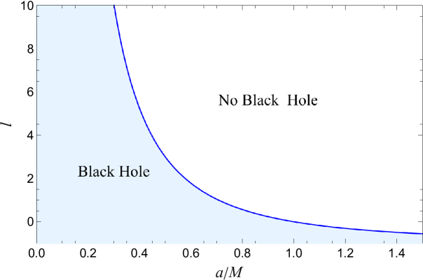
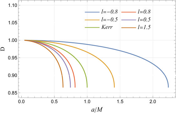
where we have defined the LSB parameter as , which takes values in the range shown in Figure 1. The metric (9) represents a purely radial Lorentz-violating solution outside a spherical body characterizing a modified black hole solution. By introducing a transformation, such that , we observe that metric (9) transforms into a Schwarzschild-like solution as:
| (10) | ||||
The metric (9) reduces to the Schwarzschild black hole without the LSB parameter, i.e., as . While static black holes are theoretical and unlikely, spinning black holes are expected to be present in the universe and can be tested through astronomical observations. We then construct a Kerr-like metric as an axisymmetric generalization of the metric (10) and validate it using EHT data. It is achieved with a modified Newman-Janis algorithm (NJA) (Azreg-A¨ınou, 2014a, b). The original Newman-Janis method (Newman and Janis, 1965) provides a groundbreaking technique to generate rotating spacetimes from a stationary, spherically symmetric initial metric without needing to solve field equations. By starting with a static and spherically symmetric black hole metric (10) and applying the modified NJA (Azreg-A¨ınou, 2014a, b), we obtain the rotating spacetime given by
| (11) | |||||
where
The black hole mass is denoted by , the LSB parameter is , and a specific spin parameter is . A non-vanishing value of results in a divergence from the Kerr solution, suggesting that the Lorentz symmetry is broken. For , we precisely recover spherical black hole (Casana et al., 2018; Ding et al., 2020)). We call the black holes represented by metric (11) as rotating black holes in Bumblebee gravity (RBHBG).
The metric(11) is singular at and at , with the singularity at is a ring-shaped physical singularity in the equatorial plane of the centre of a rotating black hole. The radial coordinate of the event horizon may be determined using the equation , much like for the Kerr spacetime. It comes out to be
| (13) |
which requires
| (14) |
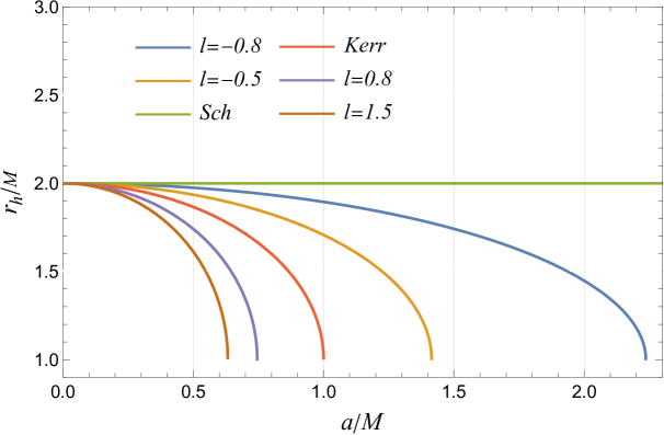
If Eq. (14) is violated, the spacetime will feature a naked singularity without an event horizon. Our study will focus exclusively on the parameter space for black holes, excluding cases involving naked singularities. Using mass as the unit, Figure 2 shows the event horizon radius as a function of spin for different values of the LSB parameter . The numerical solutions match the Schwarzschild black hole when and are zero and the Kerr black hole when is zero. Notably, for , the maximum spin parameter can exceed , while the horizon radius decreases with increasing for all . In the spherical case ( ), the event horizon remains at regardless of .
III Black hole shadow
The black hole shadow is a dark region against the bright emissions of the accretion disk, defined by the photon sphere’s boundary where the black hole’s strong-gravitational field affects light paths. Photons follow null geodesics shaped by the black hole’s mass, spin, or charge, creating a shadow surrounded by a bright photon ring (Synge, 1966; Bardeen, 1973; Luminet, 1979; Cunningham and Bardeen, 1973). This shadow reveals the spacetime structure around black holes and tests gravity theories in strong-field conditions. EHT observations are used to quantify black hole properties and assess theoretical predictions (de Vries, 2000; Shen et al., 2005; Amarilla et al., 2010; Yumoto et al., 2012; Amarilla and Eiroa, 2013; Atamurotov et al., 2013; Abdujabbarov et al., 2016, 2015; Cunha and Herdeiro, 2018; Mizuno et al., 2018; Mishra et al., 2019; Shaikh, 2019; Kumar et al., 2020; Kumar and Ghosh, 2020; Kramer et al., 2004).
| Kerr Black Hole | ||||||
|---|---|---|---|---|---|---|
| 0. | 3. | 3. | 3. | 3. | 3. | 3. |
| 0.1 | 3.11335 | 2.88219 | 3.10157 | 2.89486 | 3.12396 | 2.87069 |
| 0.2 | 3.22281 | 2.75919 | 3.2 | 2.78564 | 3.24331 | 2.73505 |
| 0.3 | 3.32885 | 2.63003 | 3.29562 | 2.67167 | 3.35864 | 2.59173 |
| 0.4 | 3.43184 | 2.49336 | 3.3887 | 2.55209 | 3.47042 | 2.43884 |
| 0.5 | 3.53209 | 2.3473 | 3.4795 | 2.42572 | 3.57904 | 2.27349 |
| 0.6 | 3.62985 | 2.18891 | 3.5682 | 2.29087 | 3.6848 | 2.09092 |
| 0.7 | 3.72535 | 2.01333 | 3.65498 | 2.14502 | 3.78798 | 1.88212 |
| 0.8 | 3.81876 | 1.81109 | 3.74 | 1.984 | 3.8888 | 1.6251 |
| 0.9 | 3.91027 | 1.55785 | 3.82337 | 1.8 | 3.98745 | 1.2 |
To find the null geodesics of photons in the RBHBG spacetime, we use the Hamilton-Jacobi equation (Carter, 1968; Chandrasekhar, 1985). The metric (11) is invariant under time translation and rotation, leading to conserved quantities such as energy and axial angular momentum . Therefore, we can determine the first-order differential equations of motion from the four integrals of motion: the Lagrangian, energy , axial angular momentum , and the Carter constant (Carter, 1968; Chandrasekhar, 1985).
| (15) | |||||
| (16) | |||||
| (17) | |||||
| (18) |
where and , respectively, pertain to the following radial and polar motion effective potentials:
| (19) | |||||
| (20) |
The Carter constant and the separability constant are related by (Carter, 1968; Chandrasekhar, 1985), reflecting the isometry of Equation (11) along the second-order Killing tensor field. While and are linked to spacetime symmetries, the Carter constant is not. The constants and govern the and motions, respectively. When , photons are restricted to an equatorial plane. Unlike Schwarzschild black holes, which have planar null circular orbits due to spherical symmetry, rotating black holes exhibit non-planar orbits due to frame dragging.
The black hole shadow silhouette is outlined by the unstable spherical photon orbits, which can be determined by solving from Eqs. (17) and (19). The radii of the photon orbits is positive root of the following equations:
| (21) |
To proceed further, following Chandershaker ((Chandrasekhar, 1985)), we can introduce the dimensionless parameters to reduce the degree of freedom of photons geodesics to one. Solving Eq. (21) for Eq. (19) results in the critical impact parameters as follows: (Chandrasekhar, 1985)
| (22) |
Here, ′ denotes the derivative with respect to the radial coordinate. In the limit , Eq. (III) reduces to the critical impact parameter for the Kerr black hole (Chandrasekhar, 1985). Light rays from a strong source follow three trajectories: (i) capture orbit, (ii) scatter orbit, and (iii) unstable orbit. The black hole’s shadow is formed by light beams falling into the black hole, with unstable photon orbits marking the boundary between capture and scatter regions. At the equatorial plane, there are two types of circular photon orbits: prograde, moving in the same direction as the black hole’s rotation, and retrograde, moving in the opposite direction. Due to the Lense-Thirring effect, prograde orbits are closer to the black hole than retrograde orbits, as the rotation of spacetime reduces the effective gravitational force in the direction of the spin. The radii of the prograde () and retrograde () orbits are obtained as roots of , leading to the following equation
| (23) |
The two primary solutions of the Eq. (23), which represent the radii of the prograde and retrograde photon orbits , respectively, are given by
| (24) |
|
|
|
|
|
|
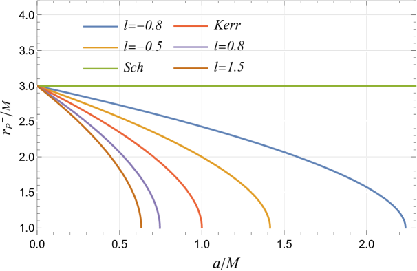
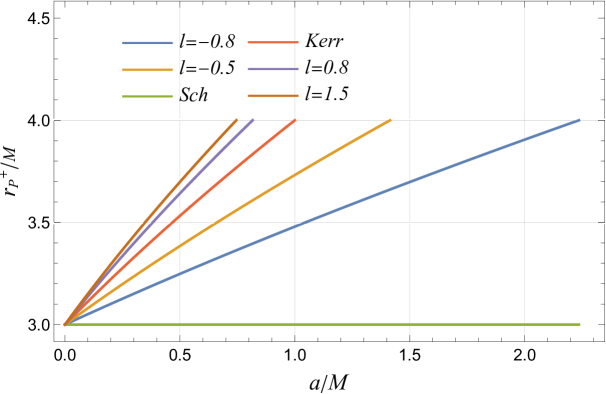
The photon orbits and vary inversely with the parameter , where decreases and increases as changes. In Bumblebee gravity, the LSB parameter introduces deviations from GR, affecting the black hole metrics. Table 2 shows the photon sphere radii and , highlighting how Lorentz violation influences the photon sphere structure. As increases, increases while decreases (cf. Figure 3 and Table 2). Compared to Kerr black holes at a constant , is lower for RBHBG when and higher otherwise, while is greater for RBHBG when and smaller otherwise (cf. Table 2). Photon orbit radii in RBHBG, like Kerr black holes, depend explicitly on spin and, for all , range from and (cf. Figure 3). Additionally, non-planar photon orbit radii for RBHBG fall within .
III.1 Shadow Silhouette
Plotting the black hole silhouette involves visualizing the apparent boundary of a black hole as seen from a distance, often referred to as the photon sphere. This shadow is defined by photons on the edge of being captured by the black hole’s gravitational pull but manages to escape. The shape of the silhouette is affected by the black hole’s spin (or angular momentum) and the angle of observation or inclination. Using the tetrad components of the four momentum and geodesic Eqs. (15),(16), (17) and (18), a relationship between the observer’s celestial coordinates, and , and two constants, and is deduced as follows
| (25) |
where
| (26) |
The coordinates and in Eq. (25) represent the apparent displacement along the perpendicular and parallel axes to the projected axis of the black hole symmetry, respectively. Therefore, an individual can visually perceive the stereographic projection of the black hole’s shadow, which is determined by the celestial coordinates specified by Bardeen (Bardeen, 1973), at an infinite radial distance () and an inclination angle of as
| (27) |
For an observer in the equatorial plane (), Eq. (27), reduces to
| (28) |
and whereas for , Eq. 28, reduces to
| (29) |
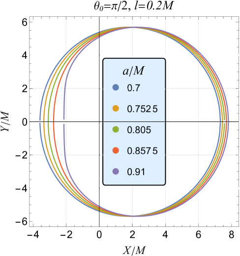
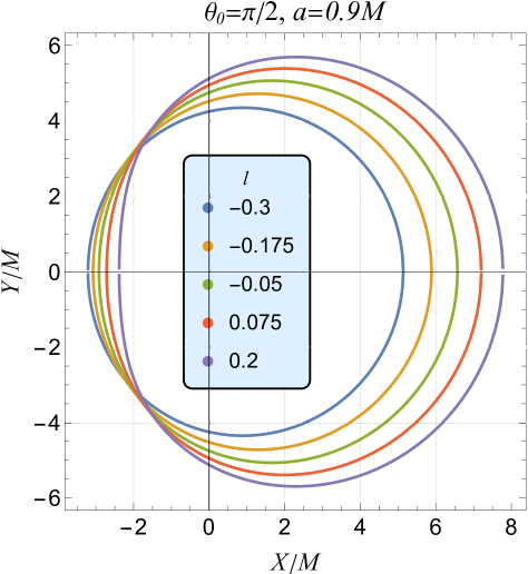
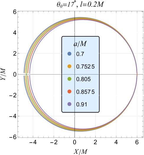
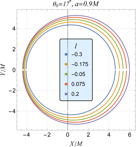
which is exactly same as obtained for the Kerr black hole (Hioki and Maeda, 2009). The parametric plots of Eq. (27) provide a Schwarzschild-like shadow for , with the contour given by . The shadow of nonrotating black holes in Bumblebee gravity is larger than that of Schwarzschild black holes and increases with . Figure 4 illustrates the RBHBG spacetime shadow silhouette for various parameter values. As increases, the shadow size grows and becomes distorted for a fixed spin . The shadow shifts horizontally along the -axis with increasing inclination angle and spin . Unlike Kerr black holes, where the shadow center is always positive, in RBHBG, the center can be negative for small values of
IV Parameter Estimation of black holes
The motivation for parameter estimation of black holes is rooted in testing and constraining fundamental theories of gravity, including the ”no-hair theorem,” which posits that black holes are fully described by just three parameters: mass, spin, and charge (Israel, 1967, 1968; Carter, 1971; Misner et al., 1973). We can challenge or refine the no-hair theorem by estimating these parameters and exploring deviations, such as Lorentz symmetry breaking or other modifications beyond GR (Israel, 1967). Observational data from instruments like the Event Horizon Telescope (EHT) (Akiyama et al., 2019a) offer a unique opportunity to investigate black holes in extreme conditions, validate theoretical models, and potentially uncover new physics that challenges conventional assumptions. Precise parameter estimation thus plays a crucial role in advancing our understanding of black hole behaviour and the nature of spacetime.
The black hole shadow (Figure 4) is a critical observable that reveals the black hole’s properties and spacetime geometry. Scientists can test GR, explore alternative gravity theories, and constrain deviation parameters by measuring its shape and size. As shown earlier, the black hole’s rotation and the LSB parameter introduce asymmetry in the shadow, with higher spin and values causing increased distortion. In Bumblebee gravity, a crucial result is the ability to estimate the parameter through observational data.
First, we employ the method proposed by Hioki and Maeda (Hioki and Maeda, 2009) for parameter estimation using shadow observables, specifically the radius and distortion , allowing for precise determination of black hole properties through deviations in shadow size and shape. Building on this, we apply the Kumar and Ghosh method (Kumar and Ghosh, 2020), which focuses on the shadow area and oblateness . By incorporating these observables, we improve our estimates of parameters like spin and the LSB parameter . Black hole parameters can be back-estimated using prior knowledge from observing these observables. Our theoretical study seeks to regulate black hole parameters like LSB parameter . However, errors in mass and distance measurements have been accounted for in EHT results. Assuming priors on mass and distance, we find that for M87* the mass , and its distance is (Akiyama et al., 2019b) and that of SgrA* is , and its distance is (Chen et al., 2019).
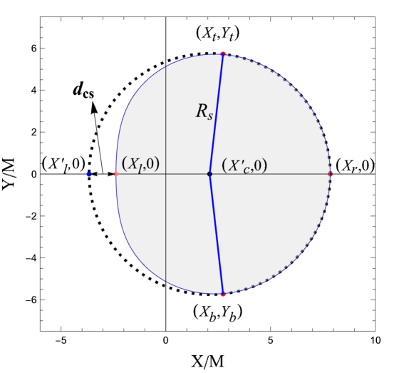
We start with defining the two observables radius and distortion , to characterize the black hole shadow silhouette as follows (Hioki and Maeda, 2009):
| (30) |
A reference perfect circle with a center that coincides with the shadow silhouette at three points, , , , to approximate the shape of the black hole shadow is drawn as shown in Figure 5. The radius of the shadow is defined by the radius of this reference circle. Further, the points , , represent the intersections of the shadow silhouette and reference circle with the horizontal axis , respectively, such that determines the potential dent on the black hole shadow in the direction perpendicular to the black hole rotational axis.
|
|
|
|
|
|
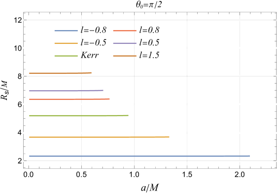
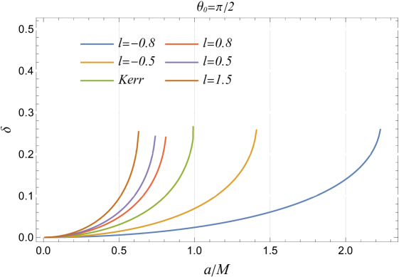
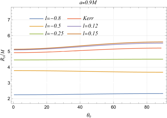
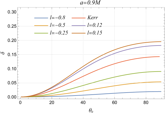
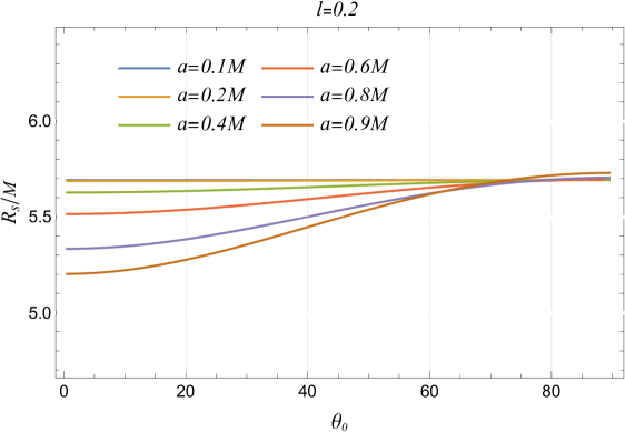
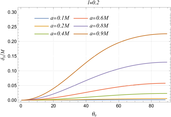
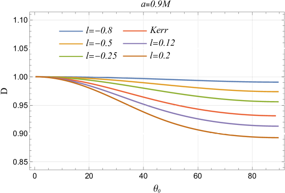
The LSB parameter consistently increases the black hole shadow radius, regardless of spin parameter or inclination angle , significantly altering black hole spacetime (cf. Figure 6). In some cases, and can overshadow the effects of spin on the shadow radius. While spin has minimal impact at fixed inclination angles, it becomes less relevant at high inclinations with spin-independent radius. At high spins, the shadow’s properties are dominated by spin, with effects being more noticeable at lower spins (cf. Figure 6). The LSB parameter primarily affects shadow distortion at high inclination angles and spins, with its impact being less noticeable at lower inclinations. At fixed inclinations, distortion is mainly influenced by spin, increasing exponentially, while both and enhance distortion at higher inclinations, though their effects are subdued at lower angles (cf. Figure 6).
|
|
|
|
|
|
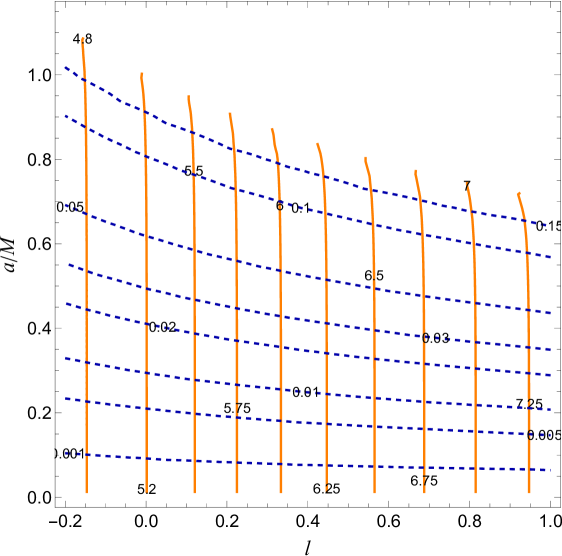
The black hole parameters are determined by combining contour plots of the radius and distortion observables, establishing a direct correlation with parameters (, ) and values (, ). With fixed black hole mass and , and measured and , the spin parameter and LSB parameter can be accurately calculated using Figure 8 and Table 2. For instance, for a black hole viewed at an inclination of with mass and observed and , we can infer and . This method provides a reliable estimate of and .
| 5.24 | 0.01 | 0.2866 | 0.0175 |
| 5.24 | 0.14 | 0.8851 | 0.0126 |
| 5.32 | 0.02 | 0.395 | 0.0485 |
| 5.32 | 0.18 | 0.923 | 0.0404 |
| 5.44 | 0.05 | 0.5914 | 0.0936 |
| 5.44 | 0.18 | 0.9053 | 0.086 |
| 5.52 | 0.10 | 0.756 | 0.1224 |
| 5.52 | 0.18 | 0.8939 | 0.1167 |
| 5.64 | 0.08 | 0.6872 | 0.1694 |
| 5.66 | 0.005 | 0.1882 | 0.1789 |
| 5.66 | 0.10 | 0.7415 | 0.1761 |
| 82 | 0.94 | 0.8503 | 0.0229 |
| 84 | 0.96 | 0.7367 | 0.0295 |
| 86 | 0.98 | 0.5498 | 0.0343 |
| 88 | 0.94 | 0.8206 | 0.096 |
| 90 | 0.995 | 0.2823 | 0.066 |
| 90 | 0.91 | 0.8896 | 0.1447 |
| 92 | 0.91 | 0.8787 | 0.1683 |
| 92 | 0.99 | 0.3893 | 0.0935 |
| 94 | 0.95 | 0.7539 | 0.1564 |
| 96 | 0.97 | 0.6181 | 0.1596 |
| 99 | 0.99 | 0.376 | 0.1725 |
We can also employ the black hole shadow observables, the shadow oblateness (), and the area () enclosed by a black hole shadow. The observables are defined as follows:
| (31) | |||||
| (32) |
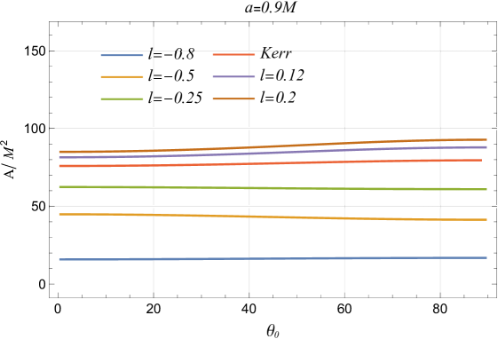
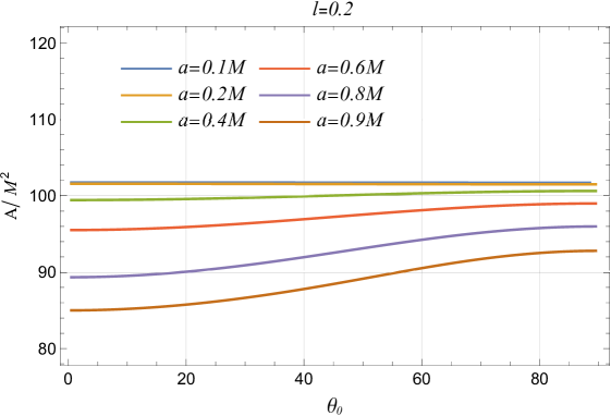
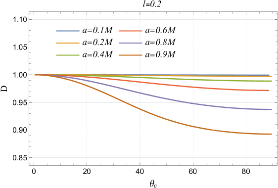
The shadow silhouette’s edges are denoted by the subscripts , , , and for the right, left, top, and bottom, respectively. For a spherically symmetric black hole, , while for a Kerr black hole, (Tsupko, 2017). The shadow area depends on the LSB parameter , spin, and . As increases, the shadow area grows if the spin and are fixed, indicating a direct impact of on the shadow size. At higher spin values, the shadow area remains stable across different inclination angles, but at lower inclinations, the shadow area varies significantly with spin when is constant. This effect diminishes at higher inclinations, suggesting that the inclination angle’s impact on the shadow area is more pronounced at lower angles (cf. Figure 7).
| -0.8 | 1.91542 | 3.43437 | 2.48985 | 4.63076 | 6.75176 | 1.45802 |
|---|---|---|---|---|---|---|
| -0.7 | 1.87006 | 3.52511 | 2.35796 | 4.41401 | 10.0762 | 2.28277 |
| -0.6 | 1.82219 | 3.6 | 2.23923 | 4.19094 | 13.3626 | 3.18844 |
| -0.5 | 1.77136 | 3.66486 | 2.12736 | 3.96039 | 16.6074 | 4.19338 |
| -0.4 | 1.71694 | 3.72264 | 2.01867 | 3.72076 | 19.8062 | 5.32315 |
| -0.3 | 1.65803 | 3.7751 | 1.91043 | 3.46982 | 22.9529 | 6.61503 |
| -0.2 | 1.5933 | 3.82337 | 1.8 | 3.20417 | 26.0395 | 8.12675 |
| -0.1 | 1.52058 | 3.86824 | 1.68416 | 2.91836 | 29.0537 | 9.95547 |
| 0.0 | 1.43589 | 3.91027 | 1.55785 | 2.60235 | 31.9754 | 12.2871 |
| 0.1 | 1.33015 | 3.9499 | 1.41032 | 2.23319 | 34.7641 | 15.567 |
| 0.2 | 1.16733 | 3.98745 | 1.2 | 1.71993 | 37.2858 | 21.6786 |
The black hole shadow’s oblateness depends on the spin, the LSB parameter , and the . At extreme spin values, the oblateness varies significantly with , becoming more elongated or less circular for larger , especially at high spin. For negative , the oblateness approaches 1, making the shadow nearly circular regardless of spin or (see Figure 7). At higher inclination angles, the oblateness deviates more from 1, while at lower angles, it remains close to 1.
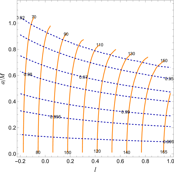
The shadow structure (Figure 4) demonstrates that both and significantly impact the shadow area and oblateness. Observing only one shadow observable, either or , can lead to ambiguities in parameter estimation. However, using both observables () allows for accurate determination of at least two parameters, as shown in Table 3 and Figure 9. Confirming these observables enables precise estimation of the spin and values for a given mass and inclination.
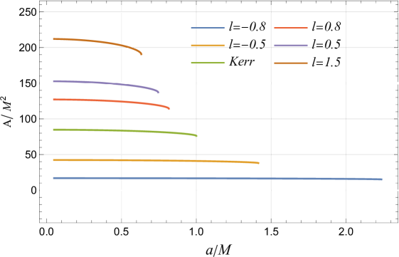
An important finding is the relationship between the shadow area and the actual black hole size, represented by the event horizon area. As the LSB parameter increases, the event horizon area decreases while the shadow area increases. This counterintuitive result suggests that while the black hole’s actual size shrinks, the perceived size of its shadow grows. This discrepancy provides insights into how the LSB parameter affects black hole spacetime, which profoundly impacts its geometric structure and gravitational projection into space.
| Observational Tests | Estimated value of | References |
|---|---|---|
| Advance of perihelion | Ref. (Casana et al., 2018) | |
| Bending of light | Ref. (Casana et al., 2018) | |
| Time delay of light | Ref. (Casana et al., 2018) | |
| GRO J1655-40 | Ref. (Wang et al., 2022) | |
| XTE J1550-564 | Ref. (Wang et al., 2022) | |
| GRS 1915+105 | Ref. (Wang et al., 2022) | |
| NuSTAR data of EXO 1846-031 | Ref. (Gu et al., 2022) | |
| EHT DATA of M87* () | Ref. (Wang and Wei, 2022) | |
| EHT DATA of M87* () | Ref. (Wang and Wei, 2022) |
V Constraints from the EHT Observation
A black hole shadow provides a direct diagnostic of strong-field gravity by revealing the black hole’s influence on spacetime. This silhouette is created by the black hole’s intense gravitational field bending and capturing light against the bright accretion disk (Jaroszynski and Kurpiewski, 1997; Falcke et al., 2000). The Event Horizon Telescope (EHT) has captured the first images of black hole shadows, including those of M87* and Sgr A*, enabling precise tests of gravitational theories (Akiyama et al., 2019a, 2022a). These observations have tightly constrained the size and shape of black hole shadows, providing valuable data for testing General Relativity (GR) and alternative gravity theories in strong-field regimes. By comparing shadow observables with EHT data, we can explore black holes in Bumblebee gravity, enhancing our understanding of gravity under extreme conditions and potentially uncovering new physics beyond GR. Previous attempts to constrain the Lorentz symmetry breaking (LSB) parameter include (Wang et al., 2022; Gu et al., 2022; Casana et al., 2018; Wang and Wei, 2022). Notably, Ref. (Wang et al., 2022) constrained black hole properties such as spin and the LSB parameter introduced by the bumblebee field, comparing Einstein-bumblebee theory predictions for quasi-periodic oscillation frequencies with observational data. Additionally, spectral data from X-ray emissions, such as the 2019 NuSTAR observation of the Galactic black hole EXO 1846-031, were used to test Einstein-bumblebee theory (Gu et al., 2022). This analysis revealed a strong degeneracy between the LSB parameter and the black hole spin, indicating that variations in one could mimic changes in the other. This degeneracy underscores the need for additional data or methods to independently estimate the black hole spin and effectively test Lorentz symmetry breaking.
EHT observations can test black hole properties in Bumblebee gravity by analyzing shadow observables such as the shadow angular diameter, Schwarzschild radius deviation, and circularity deviation. High-resolution images of Sgr A* and M87* by EHT are crucial for these analyses. Deviations in the shadow angular diameter from GR predictions can reveal the influence of the vector field in Bumblebee gravity. The angular diameter is defined as:
| (33) |
where is the shadow area and is the distance from Earth. Deviations from the Schwarzschild radius, representing the idealized size of a black hole shadow in Schwarzschild spacetime, can indicate deviations from general relativity. The Schwarzschild shadow deviation () measures the difference between the shadow angular diameter of the rotating black hole in Bumblebee gravity and the diameter of a Schwarzschild black hole. This deviation helps quantify how Lorentz-violating effects alter the black hole shadow and provides insights into modifications to spacetime structure caused by the LSB parameter (Akiyama et al., 2022a, b)
| (34) |
The Schwarzschild shadow deviation for a Kerr black hole with ranges from to as the inclination varies from to . The shadows of RBHBG can vary in size depending on the vector field and spacetime.
The circularity deviation, , measures how much a black hole’s shadow deviates from a perfect circle, offering insights into the symmetry of its gravitational field. The shadow boundary is described in polar coordinates as , where is the radial distance to the boundary and is the polar angle. The center of the shadow is at , with computed as and for symmetry along the Y-axis. The circularity deviation quantifies how much deviates from the average shadow radius , calculated as the root-mean-square deviation. The formula for is given by (Johannsen and Psaltis, 2010; Johannsen, 2013; Kumar et al., 2020):
| (35) |
where is the shadow average radius defined as (Johannsen and Psaltis, 2010)
| (36) |
Here, is the polar angle defined by , and is the radial distance from the shadow’s center to any boundary point . The observable measures the deviation of the shadow from a perfect circle. While a perfect circle has , deviations occur due to factors like the black hole’s spin, the LSB parameter in Bumblebee gravity, or the inclination angle . These deviations reveal how the black hole’s gravitational field and spacetime geometry influence the shadow’s shape, providing insights into gravity in strong-field regimes and testing alternative theories involving Lorentz violation.
EHT constraints from M87*:
The EHT measurements of the shadow angular size for M87* have provided crucial insights into the nature of black holes (Akiyama et al., 2019a). Based on a priori known estimates for the mass and distance from stellar dynamics, these measurements were primarily compared against a large library of synthetic images generated from general-relativistic magnetohydrodynamics (GRMHD) simulations of accreting Kerr black holes. This extensive comparison enabled the EHT to derive a posterior distribution for the angular radius. Through meticulous analysis, the EHT team was able to determine that the angular radius of the shadow to be approximately . The uncertainty is expressed with a 68% confidence level (Akiyama et al., 2019a).

|

|
A rigorous comparison with non-Kerr black hole solutions would ideally require building similar libraries of synthetic images from GRMHD simulations specific to those non-Kerr models. However, creating these equivalent libraries is computationally unfeasible due to the vast parameter space and the complexity involved in such simulations. Moreover, the necessity of this approach is questionable in practice. Recent comparative analysis (Mizuno et al., 2018; Vincent et al., 2021) has demonstrated that the synthetic image libraries for Kerr and non-Kerr solutions would be very similar and essentially indistinguishable from the current observational quality. This similarity arises because the differences in the shadow angular sizes for Kerr and non-Kerr black holes are minimal compared to the observational uncertainties. Therefore, we adopt the working assumption that the uncertainty in the shadow angular size for non-Kerr solutions is very similar to that for Kerr black holes. This allows us to employ the constraints derived for Kerr black holes for all the solutions considered. This approach simplifies the analysis while remaining consistent with the available observational data and theoretical predictions. Therefore, it is appropriate and timely to assess the viability of the RBHBG using the M87* black hole shadow observations. By examining the deviation from the circularity of the black hole shadow and the angular diameter, we establish constraints on the RBHBG parameters. This analysis confirms whether the RBHBG model is suitable for describing the M87* black hole, ensuring it matches the observed characteristics.
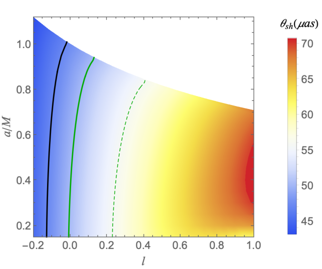
The parameter constraints for RBHBG, derived from the black hole shadow angular diameter measurements within the bound (), reveal significant insights into the allowed values for the LSB parameter . The angular diameter constraint places a bound on that varies with the spin parameter ; for example, at , is constrained to the range of to (see Figure 10 and Table 6). Notably, the EHT observations do not constrain the spin parameter , allowing flexibility in its value. Within this constrained parameter space, the M87* black hole can be described by the RBHBG spacetime model, suggesting that these black holes are strong candidates for astrophysical black holes. Furthermore, as illustrated in Figure 12, the circularity deviation bound is satisfied across the entire parameter space for an inclination angle of , indicating that the shadows of RBHBG are nearly circular at small inclination angles, which aligns well with the observational constraints for M87*.
EHT constraints from Sgr A*:
The EHT collaboration released the first image of Sgr A*, showing a compact emission region with variability on intrahour timescales (Akiyama et al., 2022c, d, e, f, a, b). Numerical simulations suggest this image matches the expected appearance of a Kerr black hole with a mass of about and a distance of , aligning with precise astrometric measurements of S-star orbits (Ghez et al., 2003, 2008; Gillessen et al., 2009). EHT models indicate an inclination angle of around and a spin parameter (Fragione and Loeb, 2020), ruling out high-inclination and non-spinning scenarios. Given its high curvature regime and accurate mass-to-distance ratio estimates, Sgr A* is an ideal target for testing astrophysical black hole models. We will use EHT data on the shadow angular diameter and Schwarzschild shadow deviation to constrain the parameters of the RBHBG model.
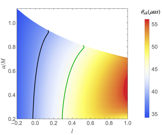
The analysis of parameters for RBHBG, based on the black hole shadow angular diameter , shows that the range , within the region for the Sgr A* shadow diameter, accommodates a broad parameter space for the RBHBG model (see Figure 11). However, more stringent constraints are provided by the EHT, which, using imaging algorithms eht-imaging, SIMLI, and DIFMAP, determines a narrower range of . This tighter range imposes significant constraints on the LSB parameter , whose extremal values depend on the spin parameter . For instance, at , is constrained between and , while at , it ranges from to ( cf. Table 6).
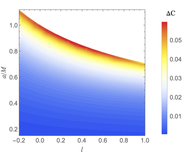
Furthermore, upper bounds on deviations from the Schwarzschild radius provided by the Keck and VLTI observations i.e., and , respectively, suggest that for and for (cf. Figure 13 and Table 6). Within these constrained parameter ranges, the RBHBG model’s shadow is consistent with the Sgr A* shadow observed by the EHT.
| EHT Observations | ||||||||
|---|---|---|---|---|---|---|---|---|
| -0.01457 | -0.0037 | 0.01156 | 0.0334 | 0.0665 | 0.125 | |||
| 0.1489 | 0.1672 | 0.1934 | 0.2321 | 0.2952 | 0.4567 | |||
| -0.1215 | -0.1162 | -0.1089 | -0.09913 | -0.08548 | -0.06489 | |||
| 0.00288 | 0.01123 | 0.02267 | 0.0385 | 0.06169 | 0.1019 | |||
| - | - | - | - | - | - | - | ||
| 0.0345 | 0.0436 | 0.0563 | 0.07395 | 0.100064 | 0.14845 | |||
| -0.08835 | -0.08225 | -0.07398 | -0.0627 | -0.0468 | -0.02218 | |||
| 0.1198 | 0.1314 | 0.14754 | 0.17045 | 0.20586 | 0.2963 |
VI Conclusion
We have investigated the properties of rotating black holes within the framework of Bumblebee gravity- namely RBHBG - wherein Lorentz symmetry is spontaneously broken by the vacuum expectation value of a vector field, mainly focusing on the impact of the LSB parameter . By using high-resolution EHT observations images of Sgr A* and M87*, we have analyzed how deviations from GR manifest in the shadow characteristics of these black holes. Our findings indicate that the RBHBG model introduces notable deviations from the Kerr black hole scenario. Specifically, the parameter is found to increase the shadow radius and enhance deformation while reducing the event horizon area. This study enhances our understanding of the effects of black hole rotation and Lorentz symmetry breaking, offering insights into modified gravity theories and contributing to reconciling GR with quantum gravity.
We have demonstrated that in the RBHBG model, unlike the Kerr black hole, the maximum spin parameter can exceed the black hole mass when . The event horizon radii decrease with increasing spin for all values of . Our calculations of photon orbit radii show that as increases, the radius of retrograde photon orbits increases, while the radius of prograde photon orbits decreases. Comparing RBHBG to Kerr black holes at the same spin value, is smaller for and larger otherwise, while is larger for and smaller otherwise. For all , the photon orbit radii in RBHBG remain within the ranges and .
We employ two established techniques for parameter estimation using shadow observables, allowing us to infer black hole parameters from observational data. Our analysis shows that the parameter consistently enlarges the shadow radius, indicating significant alterations to the black hole’s spacetime. Additionally, influences shadow distortion mainly at higher inclination angles and spins, with less effect at lower angles. The shadow area exhibits distinct dependencies on , spin, and inclination angle.
Both and spin are crucial, with their effects modulated by the inclination angle , showing more pronounced differences at lower angles. The oblateness of the shadow varies notably with at extreme spin values: for larger and fixed inclination angles, it becomes significantly less than 1, making the shadow more elongated. For negative , oblateness approaches 1 regardless of spin or inclination. The key finding is that as increases, the event horizon area decreases while the shadow area increases. These results highlight new avenues for studying black hole properties and Lorentz symmetry violations. Understanding the relationship between a black hole’s actual size and its shadow could improve interpretations of observational data and refine black hole models. It underscores the importance of considering the LSB parameter in black hole metrics and its potential to transform our understanding of black hole dynamics.
We further modeled M87* and Sgr A* as RBHBG, using observational data from the EHT to test black hole properties by examining shadow observables such as shadow angular diameter, Schwarzschild radius deviation, and circularity deviation. Within the bound of , we observed that the shadow angular diameter for the M87* black hole provides a bound on that varies with the spin parameter ; for , for instance, is constrained to the range of to . The condition is met by RBHBG for all values in the parameter space of M87*. This is because the shadows of the revolving black holes are almost perfectly circular when observed from small inclination angles.
Additionally, more stringent constraints are provided by the EHT, which, using imaging algorithms eht-imaging, SIMLI, and DIFMAP, and determines a narrower range of at an inclination angle of °. This tighter range imposes significant constraints on the LSB parameter , with its extremal values depending on the spin parameter . For instance, at , is constrained between and , while at , it ranges from to . Furthermore, upper bounds are obtained using the results on deviations from the Schwarzschild radius provided by the Keck and VLTI observations which suggest that for (Keck) and for (VLTI). These results highlight the constraints that EHT observations place on the parameters of RBHBG, providing new insights into the properties of black holes and the nature of Lorentz symmetry violations in gravitational theories.
Our study highlights the importance of the LSB parameter in black hole metrics, demonstrating its potential to reshape our understanding of black hole dynamics. Incorporating this parameter reveals how deviations from standard gravitational theories can impact astrophysical observations, enhancing our insight into black hole behaviour. This approach improves our understanding of black hole physics and contributes to evaluating quantum gravity theories and the nature of spacetime at the Planck scale, offering a clearer view of the universe’s fundamental structure.
VII Acknowledgments
S.U.I would like to thank the University of KwaZulu-Natal and the NRF for the postdoctoral research fellowship. S.G.G. is supported by SERB-DST through project No. CRG/2021/005771. S.D.M acknowledges that this work is based upon research supported by the South African Research Chair Initiative of the Department of Science and Technology and the National Research Foundation.
References
- Griffiths (2008) D. Griffiths, Introduction to elementary particles (Wiley-VCH, 2008).
- Rovelli (2004) C. Rovelli, Quantum gravity, Cambridge Monographs on Mathematical Physics (Univ. Pr., Cambridge, UK, 2004).
- Schutz (1985) B. F. Schutz, A FIRST COURSE IN GENERAL RELATIVITY (Cambridge Univ. Pr., Cambridge, UK, 1985).
- Liberati (2013) S. Liberati, Class. Quant. Grav. 30, 133001 (2013), arXiv:1304.5795 [gr-qc] .
- Mattingly (2005) D. Mattingly, Living Rev. Rel. 8, 5 (2005), arXiv:gr-qc/0502097 .
- Kostelecky (2004) V. A. Kostelecky, Phys. Rev. D 69, 105009 (2004), arXiv:hep-th/0312310 .
- Bluhm (2007) R. Bluhm, PoS QG-PH, 009 (2007), arXiv:0801.0141 [gr-qc] .
- Kostelecky and Samuel (1989a) V. A. Kostelecky and S. Samuel, Phys. Rev. D 39, 683 (1989a).
- Kostelecky and Samuel (1989b) V. A. Kostelecky and S. Samuel, Phys. Rev. Lett. 63, 224 (1989b).
- Carroll et al. (2001) S. M. Carroll, J. A. Harvey, V. A. Kostelecky, C. D. Lane, and T. Okamoto, Phys. Rev. Lett. 87, 141601 (2001), arXiv:hep-th/0105082 .
- Gambini and Pullin (1999) R. Gambini and J. Pullin, Phys. Rev. D 59, 124021 (1999), arXiv:gr-qc/9809038 .
- Kostelecky and Samuel (1989c) V. A. Kostelecky and S. Samuel, Phys. Rev. D 40, 1886 (1989c).
- Bluhm and Kostelecky (2005) R. Bluhm and V. A. Kostelecky, Phys. Rev. D 71, 065008 (2005), arXiv:hep-th/0412320 .
- Bertolami and Paramos (2005) O. Bertolami and J. Paramos, Phys. Rev. D 72, 044001 (2005), arXiv:hep-th/0504215 .
- Bailey and Kostelecky (2006) Q. G. Bailey and V. A. Kostelecky, Phys. Rev. D 74, 045001 (2006), arXiv:gr-qc/0603030 .
- Bluhm et al. (2008) R. Bluhm, N. L. Gagne, R. Potting, and A. Vrublevskis, Phys. Rev. D 77, 125007 (2008), [Erratum: Phys.Rev.D 79, 029902 (2009)], arXiv:0802.4071 [hep-th] .
- Seifert (2010) M. D. Seifert, Phys. Rev. D 81, 065010 (2010), arXiv:0909.3118 [hep-ph] .
- Maluf et al. (2014) R. V. Maluf, C. A. S. Almeida, R. Casana, and M. M. Ferreira, Jr., Phys. Rev. D 90, 025007 (2014), arXiv:1402.3554 [hep-th] .
- Páramos and Guiomar (2014) J. Páramos and G. Guiomar, Phys. Rev. D 90, 082002 (2014), arXiv:1409.2022 [astro-ph.SR] .
- Assunção et al. (2019) J. F. Assunção, T. Mariz, J. R. Nascimento, and A. Y. Petrov, Phys. Rev. D 100, 085009 (2019), arXiv:1902.10592 [hep-th] .
- Escobar and Mart´ın-Ruiz (2017) C. A. Escobar and A. Martín-Ruiz, Phys. Rev. D 95, 095006 (2017), arXiv:1703.01171 [hep-th] .
- Casana et al. (2018) R. Casana, A. Cavalcante, F. P. Poulis, and E. B. Santos, Phys. Rev. D 97, 104001 (2018), arXiv:1711.02273 [gr-qc] .
- Ovgün et al. (2018) A. Ovgün, K. Jusufi, and I. Sakalli, Annals Phys. 399, 193 (2018), arXiv:1805.09431 [gr-qc] .
- Oliveira et al. (2021) R. Oliveira, D. M. Dantas, and C. A. S. Almeida, EPL 135, 10003 (2021), arXiv:2105.07956 [gr-qc] .
- Kanzi and Sakallı (2019) S. Kanzi and I. Sakallı, Nucl. Phys. B 946, 114703 (2019), arXiv:1905.00477 [hep-th] .
- Güllü and Övgün (2022) I. Güllü and A. Övgün, Annals Phys. 436, 168721 (2022), arXiv:2012.02611 [gr-qc] .
- Maluf and Neves (2021) R. V. Maluf and J. C. S. Neves, Phys. Rev. D 103, 044002 (2021), arXiv:2011.12841 [gr-qc] .
- Ding et al. (2022) C. Ding, X. Chen, and X. Fu, Nucl. Phys. B 975, 115688 (2022), arXiv:2102.13335 [gr-qc] .
- Övgün et al. (2019) A. Övgün, K. Jusufi, and I. Sakallı, Phys. Rev. D 99, 024042 (2019), arXiv:1804.09911 [gr-qc] .
- Capelo and Páramos (2015) D. Capelo and J. Páramos, Phys. Rev. D 91, 104007 (2015), arXiv:1501.07685 [gr-qc] .
- Ding et al. (2020) C. Ding, C. Liu, R. Casana, and A. Cavalcante, Eur. Phys. J. C 80, 178 (2020), arXiv:1910.02674 [gr-qc] .
- Akiyama et al. (2019a) K. Akiyama et al. (Event Horizon Telescope), Astrophys. J. Lett. 875, L1 (2019a), arXiv:1906.11238 [astro-ph.GA] .
- Wang and Wei (2022) H.-M. Wang and S.-W. Wei, Eur. Phys. J. Plus 137, 571 (2022), arXiv:2106.14602 [gr-qc] .
- Liu et al. (2019) C. Liu, C. Ding, and J. Jing, .s (2019), arXiv:1910.13259 [gr-qc] .
- Jiang et al. (2021) R. Jiang, R.-H. Lin, and X.-H. Zhai, Phys. Rev. D 104, 124004 (2021), arXiv:2108.04702 [gr-qc] .
- Li and Övgün (2020) Z. Li and A. Övgün, Phys. Rev. D 101, 024040 (2020), arXiv:2001.02074 [gr-qc] .
- Wang et al. (2022) Z. Wang, S. Chen, and J. Jing, Eur. Phys. J. C 82, 528 (2022), arXiv:2112.02895 [gr-qc] .
- Gu et al. (2022) J. Gu, S. Riaz, A. B. Abdikamalov, D. Ayzenberg, and C. Bambi, Eur. Phys. J. C 82, 708 (2022), arXiv:2206.14733 [gr-qc] .
- Azreg-A¨ınou (2014a) M. Azreg-Aïnou, Phys. Rev. D 90, 064041 (2014a), arXiv:1405.2569 [gr-qc] .
- Azreg-A¨ınou (2014b) M. Azreg-Aïnou, Eur. Phys. J. C 74, 2865 (2014b), arXiv:1401.4292 [gr-qc] .
- Newman and Janis (1965) E. T. Newman and A. I. Janis, J. Math. Phys. 6, 915 (1965).
- Synge (1966) J. L. Synge, Monthly Notices of the Royal Astronomical Society 131, 463 (1966), https://academic.oup.com/mnras/article-pdf/131/3/463/8076763/mnras131-0463.pdf .
- Bardeen (1973) J. Bardeen, “Black holes, edited by c. dewitt and bs dewitt,” (1973).
- Luminet (1979) J. P. Luminet, aap 75, 228 (1979).
- Cunningham and Bardeen (1973) C. T. Cunningham and J. M. Bardeen, Astrophys. J. 183, 237 (1973).
- de Vries (2000) A. de Vries, Classical and Quantum Gravity 17, 123 (2000).
- Shen et al. (2005) Z.-Q. Shen, K. Y. Lo, M. C. Liang, P. T. P. Ho, and J. H. Zhao, Nature 438, 62 (2005), arXiv:astro-ph/0512515 .
- Amarilla et al. (2010) L. Amarilla, E. F. Eiroa, and G. Giribet, Phys. Rev. D 81, 124045 (2010), arXiv:1005.0607 [gr-qc] .
- Yumoto et al. (2012) A. Yumoto, D. Nitta, T. Chiba, and N. Sugiyama, Phys. Rev. D 86, 103001 (2012), arXiv:1208.0635 [gr-qc] .
- Amarilla and Eiroa (2013) L. Amarilla and E. F. Eiroa, Phys. Rev. D 87, 044057 (2013), arXiv:1301.0532 [gr-qc] .
- Atamurotov et al. (2013) F. Atamurotov, A. Abdujabbarov, and B. Ahmedov, Phys. Rev. D 88, 064004 (2013).
- Abdujabbarov et al. (2016) A. Abdujabbarov, M. Amir, B. Ahmedov, and S. G. Ghosh, Phys. Rev. D93, 104004 (2016), arXiv:1604.03809 [gr-qc] .
- Abdujabbarov et al. (2015) A. A. Abdujabbarov, L. Rezzolla, and B. J. Ahmedov, Mon. Not. Roy. Astron. Soc. 454, 2423 (2015), arXiv:1503.09054 [gr-qc] .
- Cunha and Herdeiro (2018) P. V. P. Cunha and C. A. R. Herdeiro, Gen. Rel. Grav. 50, 42 (2018), arXiv:1801.00860 [gr-qc] .
- Mizuno et al. (2018) Y. Mizuno, Z. Younsi, C. M. Fromm, O. Porth, M. De Laurentis, H. Olivares, H. Falcke, M. Kramer, and L. Rezzolla, Nature Astron. 2, 585 (2018), arXiv:1804.05812 [astro-ph.GA] .
- Mishra et al. (2019) A. K. Mishra, S. Chakraborty, and S. Sarkar, Phys. Rev. D 99, 104080 (2019), arXiv:1903.06376 [gr-qc] .
- Shaikh (2019) R. Shaikh, Phys. Rev. D 100, 024028 (2019), arXiv:1904.08322 [gr-qc] .
- Kumar et al. (2020) R. Kumar, A. Kumar, and S. G. Ghosh, Astrophys. J. 896, 89 (2020), arXiv:2006.09869 [gr-qc] .
- Kumar and Ghosh (2020) R. Kumar and S. G. Ghosh, Astrophys. J. 892, 78 (2020), arXiv:1811.01260 [gr-qc] .
- Kramer et al. (2004) M. Kramer, D. C. Backer, J. M. Cordes, T. J. W. Lazio, B. W. Stappers, and S. Johnston, New Astron. Rev. 48, 993 (2004), arXiv:astro-ph/0409379 .
- Carter (1968) B. Carter, Phys. Rev. 174, 1559 (1968).
- Chandrasekhar (1985) S. Chandrasekhar, The mathematical theory of black holes (Oxford Univ. Press, Oxford, 1985).
- Hioki and Maeda (2009) K. Hioki and K.-i. Maeda, Phys. Rev. D 80, 024042 (2009), arXiv:0904.3575 [astro-ph.HE] .
- Israel (1967) W. Israel, Physical Review 164, 1776 (1967).
- Israel (1968) W. Israel, Communications in Mathematical Physics 8, 245 (1968).
- Carter (1971) B. Carter, Phys. Rev. Lett. 26, 331 (1971).
- Misner et al. (1973) C. W. Misner, K. S. Thorne, and J. A. Wheeler, Gravitation (W. H. Freeman, San Francisco, 1973).
- Akiyama et al. (2019b) K. Akiyama et al. (Event Horizon Telescope), Astrophys. J. Lett. 875, L6 (2019b), arXiv:1906.11243 [astro-ph.GA] .
- Chen et al. (2019) Z. Chen et al., Astrophys. J. Lett. 882, L28 (2019), arXiv:1908.08066 [astro-ph.GA] .
- Tsupko (2017) O. Yu. Tsupko, Phys. Rev. D95, 104058 (2017), arXiv:1702.04005 [gr-qc] .
- Jaroszynski and Kurpiewski (1997) M. Jaroszynski and A. Kurpiewski, Astron. Astrophys. 326, 419 (1997), arXiv:astro-ph/9705044 .
- Falcke et al. (2000) H. Falcke, F. Melia, and E. Agol, Astrophys. J. Lett. 528, L13 (2000), arXiv:astro-ph/9912263 .
- Akiyama et al. (2022a) K. Akiyama et al. (Event Horizon Telescope), Astrophys. J. Lett. 930, L12 (2022a).
- Akiyama et al. (2022b) K. Akiyama et al. (Event Horizon Telescope), Astrophys. J. Lett. 930, L17 (2022b).
- Johannsen and Psaltis (2010) T. Johannsen and D. Psaltis, Astrophys. J. 718, 446 (2010), arXiv:1005.1931 [astro-ph.HE] .
- Johannsen (2013) T. Johannsen, Astrophys. J. 777, 170 (2013), arXiv:1501.02814 [astro-ph.HE] .
- Vincent et al. (2021) F. H. Vincent, M. Wielgus, M. A. Abramowicz, E. Gourgoulhon, J. P. Lasota, T. Paumard, and G. Perrin, Astron. Astrophys. 646, A37 (2021), arXiv:2002.09226 [gr-qc] .
- Akiyama et al. (2022c) K. Akiyama et al. (Event Horizon Telescope), Astrophys. J. Lett. 930, L15 (2022c).
- Akiyama et al. (2022d) K. Akiyama et al. (Event Horizon Telescope), Astrophys. J. Lett. 930, L16 (2022d).
- Akiyama et al. (2022e) K. Akiyama et al. (Event Horizon Telescope), Astrophys. J. Lett. 930, L13 (2022e).
- Akiyama et al. (2022f) K. Akiyama et al. (Event Horizon Telescope), Astrophys. J. Lett. 930, L14 (2022f).
- Ghez et al. (2003) A. M. Ghez et al., Astrophys. J. Lett. 586, L127 (2003), arXiv:astro-ph/0302299 .
- Ghez et al. (2008) A. M. Ghez et al., Astrophys. J. 689, 1044 (2008), arXiv:0808.2870 [astro-ph] .
- Gillessen et al. (2009) S. Gillessen, F. Eisenhauer, S. Trippe, T. Alexander, R. Genzel, F. Martins, and T. Ott, Astrophys. J. 692, 1075 (2009), arXiv:0810.4674 [astro-ph] .
- Fragione and Loeb (2020) G. Fragione and A. Loeb, Astrophys. J. Lett. 901, L32 (2020), arXiv:2008.11734 [astro-ph.GA] .