Is Phase Shift Keying Optimal for Channels with Phase-Quantized Output?
Abstract
This paper establishes the capacity of additive white Gaussian noise (AWGN) channels with phase-quantized output. We show that a rotated -phase shift keying scheme is the capacity-achieving input distribution for a complex AWGN channel with -bit phase quantization. The result is then used to establish the expression for the channel capacity as a function of average power constraint and quantization bits . The outage performance of phase-quantized system is also investigated for the case of Rayleigh fading when the channel state information (CSI) is only known at the receiver. Our findings suggest the existence of a threshold in the rate , above which the outage exponent of the outage probability changes abruptly. In fact, this threshold effect in the outage exponent causes -PSK to have suboptimal outage performance at high SNR.
Index Terms:
Low-resolution ADCs, Phase Quantization, Channel Capacity, Phase Shift Keying, Outage ProbabilityI Introduction
The use of low-resolution analog-to-digital converters (ADCs) has recently gained significant research interest because it addresses practical problems and scalability issues in 5G core technologies such as massive data processing, high power consumption, and cost [1]. Most studies on low-resolution ADCs have been more focused on investigating the fundamental limits and practical detection strategies in the context of multiple-input multiple-output (MIMO) and millimeter wave (mmWave) systems [2, 3, 4, 5]. However, these studies did not properly address the structure of the capacity-achieving input and only analyzed performance via capacity bounds using simplified analytical models. Low-resolution receiver design requires a shift in signal/code construction since Gaussian signaling is no longer optimal in channels with quantized output [6].
Some research efforts have been invested in analyzing the capacity limits of channels with low-resolution quantization and finding the optimum signaling schemes for such channels. One of the first studies on this topic showed that binary antipodal signaling is optimal for real AWGN channel with 1-bit quantized output [7]. Extension of capacity analysis to other wireless channels with 1-bit in-phase and quadrature (I/Q) output quantization revealed that QPSK is the optimum signaling for coherent/noncoherent Rayleigh channel [8][9], noncoherent Rician channel [6], and zero-mean Gaussian mixture channel [10]. However, identifying the structure of capacity-achieving input analytically for static and fading channels with multi-bit I/Q quantization still remains an open problem [6].
Motivated by the above discussion, we aim to extend the capacity results of 1-bit I/Q quantization to multi-bit quantization. However, we shall investigate multi-bit phase quantization instead of the conventional I/Q quantization. Phase quantization ignores the amplitude component thus eliminating the necessity for automatic gain control [11]. Furthermore, phase quantizers can be easily implemented in practice using analog phase detectors and 1-bit comparators which consume negligible power (in the order of mW) [12]. Information rate of phase-quantized block noncoherent receiver has been studied before in [11] but the proponents of the study did not show the optimality of phase shift keying. Error rate analysis of low-resolution phase-modulated communication has been done for the single-input single-output (SISO) fading channel [13, 12], relay channel [14], and multiuser MIMO channel [15] but only investigated uncoded transmissions. In this work, we provide a rigourous proof that phase shift keying is indeed capacity-achieving for static channels with phase-quantized output. In fact, the analytical tractability of the 1-bit ADC case in [8, 7, 6, 9, 10] comes from the tractability of the more general multi-bit phase quantization. We then extend the analysis to phase-quantized Rayleigh fading channel with channel state information (CSI) known only at the receiver and give some insights about the outage exponent (or diversity order) of its outage probability. In particular, our numerical results reveal a threshold effect in the outage exponent when the required transmission rate of an -PSK scheme exceeds a certain value. The proofs can be found in the supplement material [16].
II System Model
We consider a discrete-time baseband model shown in Figure 1. The transmitter sends a signal which has an average power constraint . is a complex constant representing the gain and direction of the line-of-sight (LoS) component and is an additive noise. We can express the received signal prior to quantization as
| (1) |
The signal is then fed to a symmetric -bit phase quantizer to produce an integer-valued output . To be more precise, the output of the phase quantizer is if , where is given by
Due to the circular structure of the phase quantizer, the addition operation for some constitutes a modulo addition. In this quantization model, only a coarse phase information of the received signal is retained and the goal of the receiver is to reliably recover the message encoded in using the phase quantizer output, . It should be noted that the discrete-time channel model we considered implicitly assumes that the phase quantizer is symmetric and that the channel output is sampled at the Nyquist rate. However, such quantization and sampling strategy may not be optimal in some cases as pointed out in [17, 18].
We identify the probability quantities essential to express the mutual information. Suppose we define and . The conditional PDF is given by
| (2) |
Note that in the phase-quantized receiver, we discard any information on the magnitude. Suppose we represent the random variables in polar form (i.e. use and ). The probability of given is transmitted can be written as
| (3) |
where the last equality is obtained from [19, equation (10)]. is the tail probability of the standard normal distribution. The conditional PDF (or ), denoted as (or ), is given by
| (4) |
Equation (II) has no closed-form expression. However, we can still use it to identify the optimal input distribution and numerically compute the capacity of the phase-quantized system. Now, consider an input distribution with density function . With slight abuse of notation, we use and to denote and , respectively. For a given , the probability mass function (PMF) of is therefore
| (5) |
We use the above notation to emphasize that the PMF of is induced by the choice of the distribution . Given the above probability quantities, we can now express the mutual information between and as follows:
| (6) | ||||
We use the notation since the mutual information is a result of choosing a specific input distribution . All functions in this paper are in base 2 unless stated otherwise. Let . The capacity for a given power constraint is the supremum of mutual information between and over the set of all input distributions satisfying the power constraint . In other words,
| (7) |
where is the set of all input distributions which have average power less than or equal to . In the next section, we establish the properties of the capacity-achieving input distribution when is known at the transmitter.
III Capacity-achieving Input for Phase-Quantized AWGN Channel
The mutual information is concave with respect to [20, Theorem 2.7.4] and the power constraint ensures that is convex and compact with respect to weak* topology111This is the coarsest topology in which all linear functionals of of the form , where is a continuous function, are continuous. [21]. The existence of is equivalent to showing that is continuous over . The finite cardinality of phase quantizer output trivially ensures this and the proof follows closely to the method in [7, Appendix A] and [6, Lemma 1]. We first show that the optimal input distribution satisfies a certain phase symmetry. Then, we prove that should have a single amplitude level. Finally, we identify the structure of the optimal input by establishing its discreteness and locating its mass points.
III-A Optimality of -symmetric input distribution
In this subsection, we show that the optimal input distribution is -symmetric (i.e. for all ). We first prove a key lemma about the properties of .
Lemma 1.
The function (or ) satisfies the following properties:
Proof.
See [16, Section A]. ∎
Lemma 1.i states that shifting the input by corresponds to a shift in the phase quantizer output by . Meanwhile, Lemma 1.ii and 1.iii identify some symmetry of when and . The following proposition shows that the capacity is achieved by a -symmetric distribution. Thus, without loss of generality, we can simply restrict our search of in this set of input distributions.
Proposition 1.
For any input distribution , we define another input distribution as
| (8) |
which is a -symmetric distribution. Then, . Under this input distribution, is maximized and is equal to .
Proof.
See [16, Section B]. ∎
Because of Proposition 1, we consider , where is the set of all -symmetric input distributions satisfying the constraint . The capacity in (7) simplifies to
| (9) |
III-B Optimality of input with a single amplitude level
To prove that the optimal input should have a single amplitude level, we first establish two properties of .
Lemma 2.
The function is decreasing on for all .
Proof.
See [16, Section C]. ∎
Lemma 3.
The function is convex on for all .
Proof.
See [16, Section D]. ∎
The capacity in (9) can be written as
where we used Bayes’ rule in the second line to express the complex PDF as and perform the complex expectation as two real-valued expectations over and . Due to Lemma 3, Jensen’s inequality can be applied. That is,
with equality if is a constant. This means that for some -symmetric input distribution, , with two or more amplitude levels, there exists another -symmetric input distribution, , with one amplitude level that has lower than . Moreover, due to Lemma 2, for any -symmetric input distribution with amplitude , we can find another -symmetric input distribution with amplitude such that . Thus, full transmit power must be used. We formalize this result in the following proposition.
Proposition 2.
The optimum input distribution has a single amplitude level .
The capacity expression can be simplified further to
where is the set of all circular distributions with support that are -symmetric. That is,
III-C Discreteness of the Optimal Input and Location of its Mass Points
We continue with the derivation of the optimum input distribution by identifying the minimizer of the optimization problem
| (10) |
We present two lemmas about the objective function and feasible set of (10).
Lemma 4.
The set is convex and weakly compact.
Proof.
See [16, Section E]. ∎
Lemma 5.
The function
| (11) |
is convex and weakly differentiable on .
Proof.
See [16, Section F]. ∎
The combination of Lemma 4 and Lemma 5 implies that Problem (10) is a convex optimization problem over the probability space . An optimal solution should satisfy the following inequality:
where is the weak derivative222The notions of weak derivative and weakly differentiable functions are introduced in [16, Section F]. of at a point . With some manipulation, the optimality condition can be established as
where the third line follows from the definition of capacity. Finally, by applying the contradiction argument in [21, Theorem 4], we obtain
| (12) |
with equality if . We further reduce the search space by proving that the optimal input distribution is discrete with finite number of mass points. The proof closely follows the example application of Dubin’s Theorem [22] presented in [23, Section II-C].
Lemma 6.
The support set of is discrete and contains at most points.
Proof.
See [16, Section G]. ∎
Due to Proposition 1, we can limit our search of in since if is optimal, so are for . Moreover, the optimal distribution has a single mass point inside as a consequence of Lemma 6 and Proposition 1. Because the only way to place a nonzero number of mass points in a -symmetric input distribution that is less than or equal to is to have exactly one mass point at every for and for some . A -symmetric distribution cannot be achieved by using less than mass points. Moreover, these mass points should have equal amplitudes and are equiprobable to satisfy Proposition 1. We now utilize (12) in Proposition 3 to obtain the location of the optimal mass points.
Proposition 3.
The set containing the angles of the optimum mass points is given by
| (13) |
Proof.
See [16, Section H]. ∎
Simply put, Proposition 3 states that the optimal location of the mass points are at the angle bisector of the convex cones . Now that we have established the characteristics of the , we formally state in the following theorem the capacity of the system.
Theorem 1.
The capacity of a complex Gaussian channel with fixed channel gain and -bit phase-quantized output is
| (14) |
and the capacity-achieving input distribution is a rotated -PSK with equiprobable symbols given by
Proof.
The proof follows from calculating (7) using . The capacity-achieving input follows from combining Propositions 1-3 and using the transformation . ∎
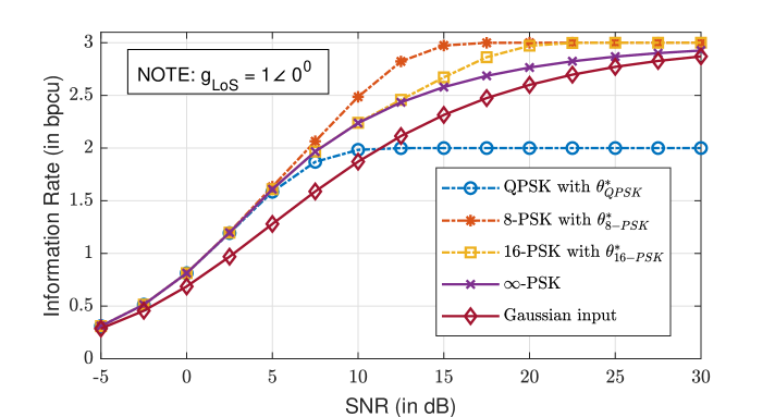
To demonstrate the optimality of the signaling scheme, Figure 2 compares the rates achieved by using 4,8,16, and -PSK (a circle) with equiprobable mass points on a Gaussian channel with 3-bit phase-quantized output. Each PSK constellation is rotated by a that maximizes the rate. The rate of Gaussian input is also included and is seen to be suboptimal compared to -symmetric input distributions with a single amplitude. It can be observed that 8-PSK with optimal achieves the highest rate among all modulation orders considered.
IV Outage Probability of Rayleigh Channel with Phase-Quantized Output
We have shown that -PSK is optimal for an AWGN channel with -bit phase-quantized output and is known at the transmitter. We now ask if this continues to hold when channel information is unavailable at the transmitter. Ultimately, is -PSK still the best choice in fading environment without channel state feedback? We now consider a quasi-static Rayleigh flat fading environment. The fixed channel gain in Figure 1 is replaced by a random fading gain . We further assume that the fading state is known only at the receiver. Without loss of generality, we assume . We define the function
as the maximum rate of reliable communication supported by a modulation scheme and a fading realization at some SNR. Here, the symbols have the form so that Propositions 1 and 2 are satisfied333We omit the proof that these necessary conditions for optimum hold even when is unknown at the transmitter.. If the transmitter encodes the data at a rate bits/channel use, then an outage occurs when since the error rate cannot be made arbitrarily small whatever coding scheme is used. The function is a convex decreasing function of (Lemmas 2 and 3). Thus, it follows that its inverse function with respect to has one-to-one mapping and is also decreasing. The outage probability is expressed as
| (15) |
The third line follows by noting that is exponentially-distributed for Rayleigh fading and is uniformly-distributed. It is difficult to analytically derive the outage probability so the expression for is evaluated numerically to provide some more insight. In order to characterize the outage probability, we focus on the outage exponent (or diversity order) which is the asymptotic slope of the outage probability as a function of SNR. Mathematically, this is defined as
| (16) |
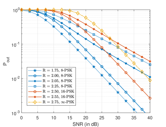
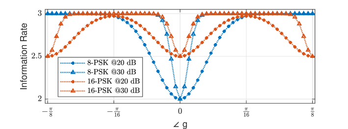
Figure 3 depicts the outage probability of Rayleigh fading channel with 3-bit phase-quantized output for different and . One noteworthy observation is the sudden decrease of the outage exponent when is increased from to for 8-PSK. DVO drops from to . This is also the case for 16-PSK when is increased from to . This can be partially explained by rates of 8-PSK and 16-PSK for varying rotations (as seen in Figure 4). Since the transmitter cannot compensate the phase rotation induced by fading, choosing an that exceeds the worst-case rates of 8-PSK and 16-PSK in Figure 4 causes outage even with high SNR. Lastly, we note that -PSK is invariant of the channel phase. As such, the choice of does not affect its outage exponent provided . However, the input distribution that achieves the best outage performance for a particular SNR and quantizer resolution still needs to be addressed by further research.
V Conclusion
In this work, we analyzed the capacity of channels with phase-quantized output. The first contribution of this work is a rigorous proof that a rotated -phase shift keying is optimal for static channels with -bit phase quantization. Using the capacity-achieving input, a channel capacity expression is established. Numerical examples were provided to demonstrate the optimality of the capacity-achieving input. For phase-quantized Rayleigh fading case, the outage performance was analyzed numerically for different -PSK modulation schemes and . Our numerical findings showed that transmitting at a rate that is above the information rate of -PSK signaling with worst-case would significantly impact the robustness of the system against outage. A threshold effect in the outage exponent was observed in 8-PSK and 16-PSK when exceeded these values. Further research needs to be conducted to be able to generalize these results to different types of fading channels. Ergodic capacity of phase-quantized fading channel is also considered for future work.
References
- [1] J. Liu, Z. Luo, and X. Xiong, “Low-Resolution ADCs for Wireless Communication: A Comprehensive Survey,” IEEE Access, vol. 7, pp. 91291–91324, 2019.
- [2] S. Jacobsson, G. Durisi, M. Coldrey, U. Gustavsson, and C. Studer, “One-bit massive MIMO: Channel estimation and high-order modulations,” in 2015 IEEE International Conference on Communication Workshop (ICCW), pp. 1304–1309, June 2015.
- [3] E. Björnson, M. Matthaiou, and M. Debbah, “Massive MIMO with Non-Ideal Arbitrary Arrays: Hardware Scaling Laws and Circuit-Aware Design,” IEEE Transactions on Wireless Communications, vol. 14, pp. 4353–4368, Aug 2015.
- [4] O. Orhan, E. Erkip, and S. Rangan, “Low power analog-to-digital conversion in millimeter wave systems: Impact of resolution and bandwidth on performance,” in 2015 Information Theory and Applications Workshop (ITA), pp. 191–198, 2015.
- [5] A. Mezghani and J. A. Nossek, “Capacity lower bound of MIMO channels with output quantization and correlated noise,” in 2012 IEEE International Symposium on Information Theory, 2012.
- [6] M. N. Vu, N. H. Tran, D. G. Wijeratne, K. Pham, K. Lee, and D. H. N. Nguyen, “Optimal Signaling Schemes and Capacity of Non-Coherent Rician Fading Channels With Low-Resolution Output Quantization,” IEEE Transactions on Wireless Communications, vol. 18, no. 6, pp. 2989–3004, 2019.
- [7] J. Singh, O. Dabeer, and U. Madhow, “On the limits of communication with low-precision analog-to-digital conversion at the receiver,” IEEE Transactions on Communications, vol. 57, pp. 3629–3639, December 2009.
- [8] A. Mezghani and J. A. Nossek, “Analysis of Rayleigh-fading channels with 1-bit quantized output,” in 2008 IEEE International Symposium on Information Theory, pp. 260–264, 2008.
- [9] S. Krone and G. Fettweis, “Fading channels with 1-bit output quantization: Optimal modulation, ergodic capacity and outage probability,” in 2010 IEEE Information Theory Workshop, pp. 1–5, 2010.
- [10] M. H. Rahman, M. Ranjbar, N. H. Tran, and K. Pham, “Capacity-Achieving Signal and Capacity of Gaussian Mixture Channels with 1-bit Output Quantization,” in ICC 2020 - 2020 IEEE International Conference on Communications (ICC), pp. 1–6, 2020.
- [11] J. Singh and U. Madhow, “Phase-quantized block noncoherent communication,” IEEE Transactions on Communications, vol. 61, no. 7, pp. 2828–2839, 2013.
- [12] S. Gayan, R. Senanayake, H. Inaltekin, and J. Evans, “Low-resolution quantization in phase modulated systems: Optimum detectors and error rate analysis,” IEEE Open Journal of the Communications Society, vol. 1, pp. 1000–1021, 2020.
- [13] S. Gayan, H. Inaltekin, R. Senanayake, and J. Evans, “Phase modulated communication with low-resolution adcs,” in ICC 2019 - 2019 IEEE International Conference on Communications (ICC), pp. 1–7, May 2019.
- [14] M. R. Souryal and H. You, “Quantize-and-forward relaying with m-ary phase shift keying,” in 2008 IEEE Wireless Communications and Networking Conference, pp. 42–47, 2008.
- [15] E. S. P. Lopes and L. T. N. Landau, “Optimal Precoding for Multiuser MIMO Systems With Phase Quantization and PSK Modulation via Branch-and-Bound,” IEEE Wireless Communications Letters, vol. 9, no. 9, pp. 1393–1397, 2020.
- [16] N. I. Bernardo, J. Zhu, and J. Evans, “Supplementary materials - proof.” https://arxiv.org/src/2101.09896/anc/supplement_mat.pdf, 2021. [Online].
- [17] T. Koch and A. Lapidoth, “At low snr, asymmetric quantizers are better,” IEEE Transactions on Information Theory, vol. 59, no. 9, pp. 5421–5445, 2013.
- [18] T. Koch and A. Lapidoth, “Increased capacity per unit-cost by oversampling,” in 2010 IEEE 26-th Convention of Electrical and Electronics Engineers in Israel, pp. 000684–000688, 2010.
- [19] H. Fu and P. Y. Kam, “Exact phase noise model and its application to linear minimum variance estimation of frequency and phase of a noisy sinusoid,” in 2008 IEEE 19th International Symposium on Personal, Indoor and Mobile Radio Communications, pp. 1–5, 2008.
- [20] T. M. Cover and J. A. Thomas, Elements of Information Theory (Wiley Series in Telecommunications and Signal Processing). USA: Wiley-Interscience, 2006.
- [21] I. C. Abou-Faycal, M. D. Trott, and S. Shamai, “The capacity of discrete-time memoryless Rayleigh-fading channels,” IEEE Transactions on Information Theory, vol. 47, no. 4, pp. 1290–1301, 2001.
- [22] L. E. Dubins, “On extreme points of convex sets,” Journal of Mathematical Analysis and Applications, vol. 5, no. 2, pp. 237 – 244, 1962.
- [23] H. Witsenhausen, “Some aspects of convexity useful in information theory,” IEEE Transactions on Information Theory, vol. 26, no. 3, pp. 265–271, 1980.
- [24] L. Alaoglu, “Weak topologies of normed linear spaces,” Annals of Mathematics, vol. 41, no. 1, pp. 252–267, 1940.