equation
| (1) |
Is Shapley Value fair?
Improving Client Selection for Mavericks in Federated Learning
Abstract
Shapley Value is commonly adopted to measure and incentivize client participation in federated learning. In this paper, we show — theoretically and through simulations— that Shapley Value underestimates the contribution of a common type of client: the Maverick. Mavericks are clients that differ both in data distribution and data quantity and can be the sole owners of certain types of data. Selecting the right clients at the right moment is important for federated learning to reduce convergence times and improve accuracy. We propose FedEMD, an adaptive client selection strategy based on the Wasserstein distance between the local and global data distributions. As FedEMD adapts the selection probability such that Mavericks are preferably selected when the model benefits from improvement on rare classes, it consistently ensures the fast convergence in the presence of different types of Mavericks. Compared to existing strategies, including Shapley Value-based ones, FedEMD improves the convergence of neural network classifiers by at least 26.9% for FedAvg aggregation compared with the state of the art.
1 Introduction
Federated Learning (FL) [40, 24, 12, 27] enables privacy-preserving learning by deriving local models and aggregating them into one global model, meaning that sensitive private data, e.g., health records, never leaves the user’s personal devices. Thus, Federated Learning allows the construction of models that cannot be computed on a central server and is hence often the only alternative for medical research and other domains with high privacy requirements.
Concretely, a central server, the federator, selects clients that train local models using their own data. The federator then aggregates these local models into a global model. This process is repeated over several global rounds, typically with different sets of clients selected in each round. Consequently, clients have to invest resources — storage, computation, and communication — into a FL system. It is essential for the federator to measure the contributions of clients’ local models. Based on the contribution, the federator can select the most suitable clients to complete the learning fast and accurately, in addition to awarding rewards based on contribution.
There exist a number of proposals for contribution measurement, i.e., algorithms that determine the quality of the service provided by the clients, for Federated Learning [16, 1, 28, 33, 23, 31, 36, 29, 37]. In particular, previous work established that Shapley Value, which measure the marginal loss caused by a client’s sequential absence from the training, offer accurate contribution measurements. Yet, the prior art of contribution measurement focused on identical and independently distributed (i.i.d.) data [33]. Here, i.i.d. refers to i.i.d. data distributions whereas the data quantity can be heterogeneous. The assumption of i.i.d. is quite limiting in practice. For example, in the widely used image classification benchmark, Cifar-10 [18], most people can contribute images of cats and dogs. However, deer images are bound to be comparable rare and owned by few clients. Another relevant example arises from learning predictive medicine from clinics who specialize in different kinds of patients, e.g., AIDS and Amyotrophic Lateral Sclerosis, and own data of exclusive disease type.
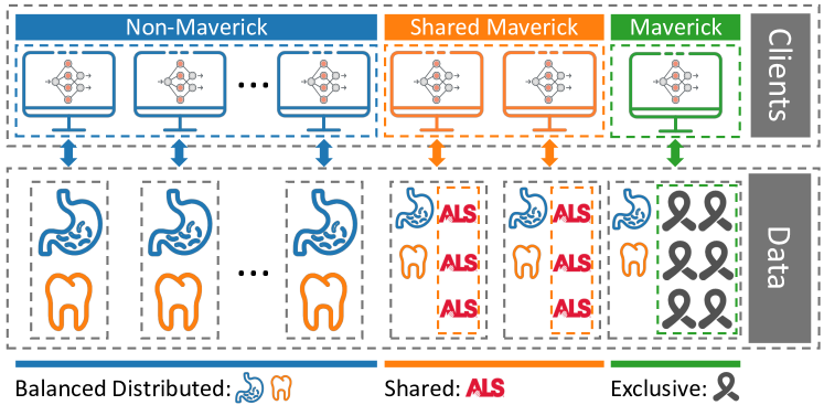
We call such clients, who hold data sets from a majority of a subset of classes, Mavericks. Fig. 1 illustrates the different distributions: In a balanced distribution, all clients own data from all classes. If a system has Mavericks, they own one or more classes (almost) exclusively whereas the non-Maverick clients have a balanced distribution for the remaining classes. Multiple Mavericks could own separate classes or jointly own one class. The latter is referred to as Shared Mavericks. Mavericks are essential to learn high-quality global models in FL. Without Mavericks, it is impossible to achieve high accuracy on the classes for which they own the majority of all training data. Such classes could be, e.g., rare deceases, which can hence only be successfully classified if Mavericks are included.
Hypothesis on the Impact of Mavericks. While Shapley Value is shown to be effective in measuring contribution for the i.i.d. case, it is largely unknown if Shapley Value can assess the contribution of Mavericks fairly and effectively involve them via the selection strategy. In order to form a hypothesis, we first conduct experiments of learning a neural network classifier (See 3 in Supplement). It shows that random and Shapley Value-based selection both perform well in the scenarios that they are designed for. Yet, they both exhibit slow convergence for Mavericks, with Shapley Value not showing a clear advantage over the random selection. This result leads us to conjecture that Shapley Value is unable to fairly evaluate Mavericks’ contribution. Moreover, this example calls for a novel client selection strategy that can handle Mavericks appropriately.
Contributions. The initial experimental study motivates the two contributions of our paper: i) a thorough theoretical analysis that shows that indeed Shapley Value-based contribution measurements underestimate the contribution of Mavericks, and ii) FedEMD, a novel client selection based on the Wasserstein distances of a user’s data distribution to both the other users’ distributions and the global distribution.
Concretely, the theoretical analysis proves that Mavericks received low contribution measurement scores during the initial stage of the learning process. Intuitively, the reason for these scores lies in the difference of their data and hence model updates to the global model. In latter stages of the learning process, Mavericks’ scores converge towards the scores of other users. Intuitively, the decaying learning rate and the increased focus on small improvements for individual classes explain this increase in score for Mavericks. However, adapting a fairness measure that relates data quantity to contribution score, Mavericks, who tend to own more data than others, are still treated unfairly. The theoretical analysis is hence in line with our initial experimental results. More generally, the theoretical analysis reveals that clients with a skewed data distribution or a high data amount are not treated fairly by SVB.
We propose FedEMD, a light-weight Maverick-aware selection method for Federated Learning. As Mavericks are strategically involved when they can contribute the most, the convergence speed increases, meaning that the learning process can terminate faster and more efficiently. Our emulation results show that the proposed FedEMD has faster convergence in comparison to state-of-the-art algorithms [24, 3, 25], by at least 26.9% and 11.3% respectively, under FedAvg and FedSGD aggregations for a range of Maverick scenarios.
2 Related Studies
Contribution Measurement. Existing work on contribution measurement can be categorized in two classes: i) local approach: clients exchange the local updates, i.e., model weights or gradients, and measure the contribution of each other, e.g., by creating a reputation system [16], and ii) global approach: all clients send all their model updates to the federator who in turn aggregates and computes the contribution via the marginal loss [28, 33, 23, 31, 36, 29, 37]. The main drawbacks of local approaches are the excessive communication overhead and the lower privacy due to directly exchanged model updates [1]. In contrast, the global approach has lower communication overhead and avoids the privacy leakage to other clients by communicating only with the federator. Prevailing examples of globally measuring contribution are Influence [28, 29] and Shapley Value [33, 37, 36, 30]. The prior art demonstrates that Shapley Value can effectively measure the client’s contribution for the case when clients’ data is i.i.d. or of biased quantity [30]. Yet, a recent experimental study[41] demonstrates that the correlation between a user’s data quality and its Shapley Value is limited. The results raise doubts whether Shapley Value is really a suitable choice for contribution measurement. However, there is no rigorous analysis on whether Shapley Value can effectively evaluate the contribution from heterogeneous users with skewed data distributions.
Client Selection. Selecting clients within a heterogeneous group of potential clients is key to enabling fast and accurate learning based on high data quality. The state-of-the-art client selection strategies focus on the resource heterogeneity [26, 39, 15] or data heterogeneity [3, 5, 22, 4]. In the case of data heterogeneity, which is a focus of our work, selection strategies [5, 13, 3] gain insights on the distribution of clients’ data and then select them in specific manners. Goetz et. al [13] apply active sampling and Cho et. al [5] use Power-of-Choice to favor clients with higher local loss. TiFL [3] considers both resource and data heterogeneity to mitigate the impact of straggler and skewed distribution. TiFL applies a contribution-based client selection by evaluating the accuracy of selected participants each round and choose clients of lower accuracy. FedFast [25] chooses classes based on clustering and achieves fast convergence for recommendation systems. However, there is no selection strategy that addresses the Maverick scenario.
Data Heterogeneity. As an alternative to client selection strategies, multiple methodologies have been suggested to properly account for data heterogeneity in FL systems [21, 7, 8, 11, 14]. Early solutions require the federator to distribute a shared global training set [42], which is demanding and violates data privacy. Later studies either focus on the local learning stage [22, 17] or improved aggregation [35]. For instance, FedProx [22] improves the local objective by adding an additional regularization term, whereas FedNova [35] first normalizes the local model updates based on the number of their local steps and aggregates the local models. The downside of aforementioned solutions is the requirement of additional computation on clients.
3 Fairness Analysis for Shapley Value
The objective is to rigorously and analytically answer the question if Shapley Value is a fair contribution measurement for Mavericks. First, we formalize FL, our assumptions, Maverick, and fairness. Since the main building block of Shapley Value is the Influence Index [28], we then derive the fairness of Influence Index. Further, we derive the fairness of Shapley Value from the Influence Index and show that Shapley Value-based contribution measurements underestimate the contribution of Mavericks but more generally the contribution of other clients with skewed data distributions or large amounts of data. We empirically verify the lack of fairness for Mavericks in existing contribution measurements.
Notation: In this paper, we focus on classification tasks. We denote the set of possible inputs as and the set of class labels that can be associated with the inputs as . In agreement with other works, we let assign a probability distribution of potential classes to inputs. With denoting the learned weights of the machine learning tasks, the empirical risk is for a SGD-based learning process under cross-entropy loss. Furthermore, the learning objective is then generally defined as: .
We are solving the learning objective in a Federated Learning scenario. In an FL system, there is a set of clients. Enumerate the clients selected in a round by . Each client selected in round computes local updates and the federator aggregates the results. Concretely, with being the learning rate, updates their weights in the t- global round by
| (2) |
The most common aggregation method is an average of the client updates, weighted by the amount of data one owns. Let denote the data quantity, then FedAvg aggregation is .
Assumptions: i) All parties are honest and follow the protocol. ii) Clients are homogeneous with respect to other resources, such as computation and communication. iii) The network is reliable with all messages being delivered within a maximal delay. iv) The global distribution has high similarity with the real-world (test dataset) distribution.
Definition 3.1 (Maverick).
Let be a class label that is primarily owned by Mavericks. In the extreme case, there is one Maverick but it might also be a small set of Mavericks jointly owning the same class. For a client , let be the fraction of ’s data that has label . Then:
| (3) |
Remark 1.
A system might contain more than one Maverick. We refer to Mavericks that own exclusive classes as exclusive Mavericks. If the Mavericks all own the same class, we refer to them as shared Mavericks.
The relation between being a Maverick and the amount of owned data can be essential. Learning success on a class relates closely to the amount of data available for that class. Thus, for the Maverick to have a positive contribution when they are the only one owning a class, they should own more data than others. Our evaluation hence focuses on Mavericks that own considerably more data than other clients, e.g., more than half of the data of all selected clients. However, the theoretical results regarding fairness hold as long as the Maverick owns at least the average amount of data.
Definition 3.2 (Data Size Fairness).
Denote the contribution measured for client in round as , their relative contribution ratio as , and their local data quantity ratio as . We define a system as fair for in round if the difference is small. The concrete fairness of client at round is
| (4) |
Definition 3.3 (Fairness Utility).
Fairness utility on a system level:
| (5) |
Remark 2.
From Def. 3.3, represents the ideal fairness.
Our aim is to show that Shapley Value-based contribution measures achieve a low fairness if Mavericks are involved. Concretely, we show that the value of Eq. 4 is lower if is a Maverick than if they are a non-Maverick.
3.1 Influence Index in FL
In this part, we discuss the fairness of Influence Index for clients. First, we consider the effect of data quantity on fairness, particularly for clients with a very low or high quantity of data. Second, we analyze the effect of skewed data distributions.
We use Influence Index as defined by Richardson et. al [28]: Let denote the weights at round if is excluded from the aggregation and refer to the local updates of . Then, the Influence Index of in global round is:
| (6) |
Data Size Matters: As stated above, Mavericks are likely to own a different amount of data than non-Mavericks. Thus, we first look into how the amount of data affects fairness regardless of the data distribution over classes. We relate the Influence Index from Eq. 6 to the local data quantity by considering the difference in Influence Index of two clients. Without loss of generality, let one of the clients be and assume that is not a Maverick, resulting in:
| (7) |
Extreme case: is very large: If , i.e., , it follows from Eq. 6 that
| (8) |
and hence . We argue that it is highly likely that or , i.e., the right-hand side of the equation is negative or close to 0. The difference represents the difference between ’s weights rather than weights related to the learning process, which can be expected to be high.
Initially, is likely to be large but still smaller than the completely random with high probability. It follows that . When increases, is expected to decrease while stays high, and hence indeed . As contributes much more data than , both scenarios are unfair.
Proposition 3.1.
A client with a large data quantity ratio is treated unfairly as their Influence Index is lower than others despite having a higher local data quantity.
Data Distribution Matters: Following a similar approach before, we adapt a more general notion of a skewed distribution than in Eq. 3 to obtain results that are of relevance beyond the case of Mavericks. Concretely, we define a skewed data distribution as one that differs from the global data distribution significantly, e.g., more than expected when distributing data randomly between clients. In order to analyze the impact of distributions, consider the Kullback-Leibler Divergence (KLD) [19], which measures the difference between two distributions. Let , and denote the distributions corresponding to , (global model weights) and , respectively. In a learning process, we have: , where refers to the KLD between distribution and . According to the definition of KLD and the fact that has a skewed data distribution, we have (derivation details see A.2 in Supplement):
| (9) |
Eq. 9 can also be written as . Recall Eq. 6, it indicates . As the round increases, combining , , as well as gives . It follows that the Influence Index of and are approximately equal.
Proposition 3.2.
The Influence Index is unfair towards clients with a skewed distribution in the initial phase of the training. During the later phase of the training, it increases but remains unfair towards clients with larger-than-average amounts of data.
Maverick - Size and Distribution Matters As by Eq. 3, a Maverick’s data distribution differs considerably from an expected distribution and hence counts as a skewed distribution. Thus, the results for skewed data distributions hold for Mavericks. If a Maverick owns more data than an average client, it is treated doubly unfair as by the first evaluation regarding data size.
Proposition 3.3.
Mavericks are treated unfairly, with their Influence Index being lower than that of an average client in the early stage of the learning process and being similar in the latter stage, despite their large quantity of data.
3.2 Shapley Value for Mavericks
Definition 3.4 (Shapley Value).
Let denote the set of clients selected in a round excluding , denote moving from . Shapley Value of is
| (10) |
Note that is the Influence Index on , which is defined in Eq. 6. To substitute the definition of influence index into the Shapley Value in Eq.10, we first analyze the difference of and ’s Shapley Value, similar to Sec. 3.1, resulting in (detailed derivation see A.1 in Supplement):
| (11) | ||||
with , , .
It can be concluded that the measurement of Shapley Value and Influence Index share the same trend that they are unfair to Mavericks. Note that rather than considering Influence Index for the complete set of clients, Eq. 11 only considers Influence Index on a subset . However, our derivations in Sec. 3.1 are independent from the number of selected clients and remain applicable for subsets , meaning that indeed the second and the third term of Eq. 11 are negative. Similarly, the first term is negative as the loss for clients only owning one class is higher. However, Shapley Value has better quality for clients with large data set than Influence Index since increases if the distance between ’s distribution and the global distribution is small. So, i.i.d. clients with a large data quantity are evaluated better by Shapley Value than Influence Index, in line with previous work.
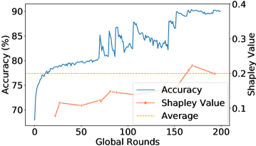
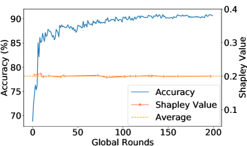
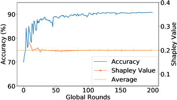
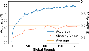
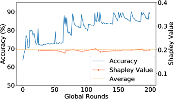
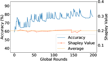
Empirical Verification: We present the empirical evidences of how one or multiple Mavericks impact the global accuracy for an Shapley Value-based contribution measure. We consider 1,2, or 3 Mavericks. If more than 1 Maverick is considered, both exclusive and shared Mavericks are evaluated. Hence, a Maverick owning a single class has considerably more data than non-Mavericks. We use Fashion-MNIST (2a) and Cifar-10 (2d) as learning scenarios, with details in Sec. 5.
Fig. 2 shows the global accuracy and the relative Shapley Value during the training, with the average relative Shapley Value of the 5 selected clients indicated by the dotted line. The contribution is only evaluated when a Maverick was selected. Fig.(2a), (2d) confirm Proposition 3.3. For more Mavericks, the measured contribution is close to the average, as indicated in Fig.(2b),(2c),(2e), and(2f). Looking at the global accuracy for all scenarios, we see a fast increase with Mavericks, meaning that the initial phase during which the Maverick’s contribution is lower than average is essentially non-existent. As even shared Mavericks own more data than non-Mavericks, an average Shapley Value remains unfair.
4 FedEMD
Here, we propose the novel client selection algorithm FedEMD, which enables FL systems with Mavericks to achieve faster convergence. First, we have established a trivial solution to empirically show that involving Mavericks in every round does not result in better accuracy. Quite the contrary, always including a Maverick has a detrimental effect in the long run.(See A.4 in Supplement). Further, we design FedEMD based on the Wasserstein Distance (EMD) [2] of client data distributions as a light-weight dynamic client selection strategy.
Overview. FedEMD (summarized in Alg. 1) selects clients each round using weighted random sampling, where the weights of each client are dynamically updated every round. To obtain the weights, we compute the global and current Wasserstein distance for each client. We structure FedEMD in three steps : i) Distribution Reporting and Initialization (Line 2–7): Clients perform distribution profile reporting so that the federator is able to sum up the global distribution and initialize the current distribution. ii) Dynamic Weights Calculation (Line 10–18): In this key step, we utilize a light-weight measure based on EMD to calculate dynamic selection probabilities over time, which achieve faster convergence, yet avoid overfitting. iii) Weighted Client Selection (Line 19–23): According to the probabilities computed in the previous step, FedEMD applies weighted random sampling to select clients.
Motivation of choice of Wasserstein Distance: FedEMD considers both global and current distance on client data distribution to increase the chance of selecting Mavericks at the early stages and profit from their diverse data. Later on, the selection probability is reduced to avoid skewing the distribution towards the Maverick classes. To measure the distance of distributions, the weight divergence defined by [42] of and is:
| (12) |
Note that is the EMD of and the global distribution, which directly leads to the drift of by . Thus, we use EMD as the distance measure in our distribution-based FedEMD (Design principle and details see A.5 in Supplement).
Dynamic Weights Calculation: Let be the EMD of distributions between and and be the self-reported data distribution matrix of clients. It is only reported once at the beginning of the learning. Also, we assume a limit of on the global communication rounds. The dynamic selection probability of clients in round , , is based on both the global distance and current distance between the local distribution and the global/current , (Line 23). Assume that is one class randomly chosen by federator except for the Maverick class111the federator can tell from the reported data distributions which classes are Maverick classes from , here we apply normalization method for distributions (Line 7, 21). The current distribution is the accumulated of selected clients over rounds (Line 18).
Distance-based Aggregation: The larger is, the higher the probability that a client is selected, since brings more distribution information to train . However, the current distance is also taken into consideration to improve the selection of Mavericks. Therefore, for in round , where is the distance coefficient to weigh the global and current distance. shall be adapted for different initial distributions, i.e., different dataset and distribution rules (See A.10 in Supplement). Clients with larger global distance and smaller current distance have a high probability to be selected, and thus Mavericks are involved more often during the early period and less later on of training to gain faster convergence. The sampling procedure for selecting clients based on (Line 9–17) has complexity of [9], so comparably low.
5 Experimental Evaluation
In this section, we evaluate the convergence speed of FedEMD in comparison to four state-of-the-art selection strategies and FedProx as the representative of SOTA algorithm for data heterogeneity. The evaluation considers four different classifiers and two Maverick types.
Datasets and Classifier Networks We use public image datasets: i) Fashion-MNIST [38] for bi-level image classification; ii) MNIST [20] for simpler tasks which need less data to do fast learning; iii) Cifar-10 [18] for more complex task such as colored image classification; iv) STL-10 [6] for applications with small amounts of local data for all clients. We note that light-weight neural networks are more applicable for federated learning scenarios, where clients typically have limited computation and communication resources [25]. Thus, here we apply light-weight CNN for each dataset correspondingly, neural network details are provided in A.9 in Supplement.
Federated Learning System The system considered has 50 participants with homogeneous computation and communication resources and 1 federator. At each round, the federator selects 5 (a common practise in related studies [32]) clients according to a client selection algorithm. The federator uses FedSGD or FedAvg to aggregate local models from selected clients. As FedSGD always considers one local epoch, we choose the same for FedAvg to enable a fair comparison of the two approaches. Two types of Mavericks are considered: exclusive and shared Mavericks. We consider the case of single Maverick owning an entire class of data in most of our experiments.
Evaluation Metrics i) Global test accuracy for all classes; ii) Source recall (related results see A.4 in Supplement) for classes owned by Mavericks exclusively; iii) : the number of communication rounds required to reach 99% of test accuracy of random selection based results; iv) Normalized Shapley Value ranging between to measure the contribution of Mavericks; 5) Computation time (results see A.7 in Supplement): the computation time measured by the federator, including training, aggregation and client selection time.
Baseline We consider four selection strategies: Random [24], Shapley Value-based, FedFast [25], and recent TiFL [3]222When implementing, we focus on their client selection and leave out other features. For example, we do not implement the features related to the communication acceleration in TiFL and the aggregation in FedFast. under both FedSGD and FedAvg aggregation methods. Although Shapley Value itself is a contribution measure rather than client selection strategy, it has been widely adopted in incentive design to attract the participants of clients with high Shapley Value [30]. Thus, the Shapley Value-based algorithm here is a variant of weighted random selection whose weights are decided by the relative Shapley Value, i.e., the probability of a client to be selection corresponds to their relative Shapley Value. Further, in order to compare with state-of-the-art solution for heterogeneous FL which focus on the optimization design, we evaluate FedProx [22] as one of the baselines.
5.1 Convergence Analysis for Selection
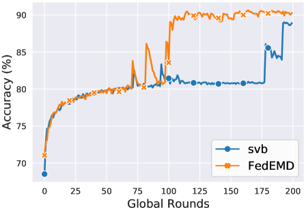
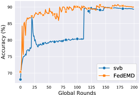
Fig. 3 shows the change in global accuracy over rounds. FedEMD achieves an accuracy close to the maximum almost immediately for FedAvg while SVB requires about 100 rounds. For FedSGD, both client selection methods have a slower convergence but FedEMD still only requires about half the number of times to achieve the same high accuracy as SVB. The reason for the result lies in SVB rarely selecting the Maverick in the early phase of the training, as, by Sec. 3, the Maverick has a below-average Shapley Value.
Furthermore, let us zoom into the number of rounds needed to reach 99% of max accuracy. Combining these results with random selection, we see that it takes 72 and 104 rounds to reach for SVB and FedEMD in FedAvg, respectively while SVB fails in reaching within 200 rounds.
Comparison with baselines. We summarize the comparison with the state-of-the-art methodologies in Table 1. The reported is averaged over three replications. Note that we run each for 200 rounds, which is mostly enough to see the convergence statistics for these lightweight networks. The rare exceptions when 99% maximal accuracy is not achieved for random selection are indicated by , e.g., when FedFast fails in most of evaluations for Maverick.
Thanks to its distance-based weights, FedEMD achieves faster convergence than all other algorithms consistently. The reason for such result is that FedEMD enhances the participation of the Maverick during early training period, speeding up learning global distribution. For most settings, the difference in convergence speed is considerably visible.
| FedSGD | FedAvg | |||||||||
|---|---|---|---|---|---|---|---|---|---|---|
| Dataset | Random | TiFL | FedFast | FedProx | FedEMD | Random | TiFL | FedFast | FedProx | FedEMD |
| MNIST | 132.7 | 111.0 | >200 | 117.7 | 98.7 | 72.3 | 84.0 | >200 | 51.0 | 40.0 |
| FMNIST | 144.0 | 140.3 | >200 | 135.7 | 131.3 | 110.7 | 146.3 | >200 | 92.0 | 79.7 |
| Cifar-10 | 140.7 | 147.3 | >200 | 164.0 | 140.0 | 143.0 | 119.7 | 173.7 | 143.7 | 107.0 |
| STL-10 | 122.3 | 124.7 | 171.0 | 186.0 | 96.3 | 179.7 | >200 | 153.0 | 179.0 | 95.0 |
The only exception here are relatively easy tasks with simple averaging rather than weighted, e.g., Cifar-10 with FedSGD, which indicates our distribution-based client selection method is especially useful for data size-aware aggregation and more complex tasks (e.g., FedAvg). While such an increased weight caused by larger data size can lead to a decrease in accuracy in the latter phase of training, Mavericks are rarely selected in the latter phase of training by FedEMD, which successfully mitigates the effect and achieves a faster convergence.
5.2 Different Types of Mavericks
We explore the effectiveness of FedEMD on two types of Mavericks: exclusive and shared Mavericks.
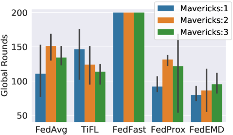
We vary the number of Mavericks between one and three and use the Fashion-MNIST dataset. The Maverick classes are ‘T-shirt’, ‘Trouser’, and ‘Pullover’. Results are shown with respect to .
Fig. 4a illustrates the case of multiple exclusive Mavericks. For exclusive Mavericks, the data distribution becomes more skewed as more classes are exclusively owned by Mavericks. FedEMD always achieves the fastest convergence, though its convergence time increases slightly as the number of Mavericks increases, reflecting the increased difficulty of learning in the presence of skewed data distribution. FedFast’s -mean clustering typically results in a cluster of Mavericks and then always includes at least one Maverick. As shown in A.5 in Supplement, constantly including a Maverick hinders convergence, which is also reflected in FedFast’s results. TiFL outperforms FedAvg with random selection for multiple Mavericks. However, TiFL’s results differ drastically over runs due to the random factor in local testing. Thus, TiFL is not a reliable choice for Mavericks. Comparably, FedProx tends to achieve the best performance among the SOTA algorithms but still exhibits slower convergence than FedEMD because higher weight divergence entails higher penalty on the loss function.
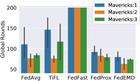
For shared Mavericks, a higher number of Mavericks indicates a more balanced distribution. Similar to the exclusive case, FedEMD has the fastest convergence and FedFast again trails the others. The improvement of FedEMD over the other methods is less visible due to the limited advantage of FedEMD on balanced data. In terms of the effectiveness of FedEMD handing more shared Mavericks, the convergence speed improves slightly. However, we attribute such an observation partially to the fact that a higher number of Mavericks resembles the case of i.i.d.. Random performs the most similar to FedEMD, as random selection is best for i.i.d. scenarios, which shared Mavericks are closer to. Note that the standard deviation of FedEMD is smaller, implying a better stability.
6 Conclusion
Client selection is key to successful Federated Learning as it enables maximizing the usefulness of different diverse data sets. In this paper, we highlighted that existing schemes fail when clients have heterogeneous data, in particular if one class is exclusively owned by one or multiple Mavericks. We proposed and evaluated an alternative algorithm that encourages the selection of diverse clients at the opportune moment of the training process, accelerating the convergence speed by up to at least 26.9% in average for multiple dataset under FedAvg aggregation, compared to the state of the art.
References
- [1] Yoshinori Aono, Takuya Hayashi, Lihua Wang, Shiho Moriai, et al. Privacy-preserving deep learning via additively homomorphic encryption. IEEE Transactions on Information Forensics and Security, 13(5):1333–1345, 2017.
- [2] Martin Arjovsky, Soumith Chintala, and Léon Bottou. Wasserstein generative adversarial networks. In International conference on Machine Learning (ICML), pages 214–223. PMLR, 2017.
- [3] Zheng Chai, Ahsan Ali, Syed Zawad, Stacey Truex, Ali Anwar, Nathalie Baracaldo, Yi Zhou, Heiko Ludwig, Feng Yan, and Yue Cheng. Tifl: A tier-based federated learning system. In Proceedings of the 29th International Symposium on High-Performance Parallel and Distributed Computing (HPDC), page 125–136, 2020.
- [4] Zheng Chai, Hannan Fayyaz, Zeshan Fayyaz, Ali Anwar, Yi Zhou, Nathalie Baracaldo, Heiko Ludwig, and Yue Cheng. Towards taming the resource and data heterogeneity in federated learning. In 2019 USENIX Conference on Operational Machine Learning (OpML 19), pages 19–21, 2019.
- [5] Yae Jee Cho, Jianyu Wang, and Gauri Joshi. Client selection in federated learning: Convergence analysis and power-of-choice selection strategies. arXiv preprint arXiv:2010.01243, 2020.
- [6] Adam Coates, Andrew Ng, and Honglak Lee. An analysis of single-layer networks in unsupervised feature learning. In Proceedings of the fourteenth international conference on artificial intelligence and statistics (AISTATS), pages 215–223. JMLR Workshop and Conference Proceedings, 2011.
- [7] Yuyang Deng, Mohammad Mahdi Kamani, and Mehrdad Mahdavi. Distributionally robust federated averaging. In Advances in Neural Information Processing Systems (NeurIPS), 2020.
- [8] Canh T. Dinh, Nguyen H. Tran, and Tuan Dung Nguyen. Personalized federated learning with moreau envelopes. In Hugo Larochelle, Marc’Aurelio Ranzato, Raia Hadsell, Maria-Florina Balcan, and Hsuan-Tien Lin, editors, Advances in Neural Information Processing Systems (NeurIPS), 2020.
- [9] Pavlos S Efraimidis and Paul G Spirakis. Weighted random sampling with a reservoir. Information Processing Letters, 97(5):181–185, 2006.
- [10] Dominik Maria Endres and Johannes E Schindelin. A new metric for probability distributions. IEEE Transactions on Information theory, 49(7):1858–1860, 2003.
- [11] Alireza Fallah, Aryan Mokhtari, and Asuman E. Ozdaglar. Personalized federated learning with theoretical guarantees: A model-agnostic meta-learning approach. In Advances in Neural Information Processing Systems (NeurIPS), 2020.
- [12] Avishek Ghosh, Jichan Chung, Dong Yin, and Kannan Ramchandran. An efficient framework for clustered federated learning. In Advances in Neural Information Processing Systems (NeurIPS), 2020.
- [13] Jack Goetz, Kshitiz Malik, Duc Bui, Seungwhan Moon, Honglei Liu, and Anuj Kumar. Active federated learning. arXiv preprint arXiv:1909.12641, 2019.
- [14] Filip Hanzely, Slavomír Hanzely, Samuel Horváth, and Peter Richtárik. Lower bounds and optimal algorithms for personalized federated learning. In Advances in Neural Information Processing Systems (NeurIPS), 2020.
- [15] Tiansheng Huang, Weiwei Lin, Wentai Wu, Ligang He, Keqin Li, and Albert Zomaya. An efficiency-boosting client selection scheme for federated learning with fairness guarantee. IEEE Transactions on Parallel and Distributed Systems, 2020.
- [16] Jiawen Kang, Zehui Xiong, Dusit Niyato, Shengli Xie, and Junshan Zhang. Incentive mechanism for reliable federated learning: A joint optimization approach to combining reputation and contract theory. IEEE Internet Things J., 6(6):10700–10714, 2019.
- [17] Sai Praneeth Karimireddy, Satyen Kale, Mehryar Mohri, Sashank Reddi, Sebastian Stich, and Ananda Theertha Suresh. Scaffold: Stochastic controlled averaging for federated learning. In International Conference on Machine Learning (ICML), pages 5132–5143. PMLR, 2020.
- [18] Alex Krizhevsky, Geoffrey Hinton, et al. Learning multiple layers of features from tiny images. 2009.
- [19] Solomon Kullback and Richard A Leibler. On information and sufficiency. The annals of mathematical statistics, 22(1):79–86, 1951.
- [20] Yann LeCun, Léon Bottou, Yoshua Bengio, and Patrick Haffner. Gradient-based learning applied to document recognition. Proceedings of the IEEE, 86(11):2278–2324, 1998.
- [21] Qinbin Li, Yiqun Diao, Quan Chen, and Bingsheng He. Federated learning on non-iid data silos: An experimental study. arXiv preprint arXiv:2102.02079, 2021.
- [22] Tian Li, Anit Kumar Sahu, Manzil Zaheer, Maziar Sanjabi, Ameet Talwalkar, and Virginia Smith. Federated optimization in heterogeneous networks. In Proceedings of Machine Learning and Systems (MLsys), 2020.
- [23] Yuan Liu, Shuai Sun, Zhengpeng Ai, Shuangfeng Zhang, Zelei Liu, and Han Yu. Fedcoin: A peer-to-peer payment system for federated learning. CoRR, abs/2002.11711, 2020.
- [24] Brendan McMahan, Eider Moore, Daniel Ramage, Seth Hampson, and Blaise Aguera y Arcas. Communication-efficient learning of deep networks from decentralized data. In Proceedings of Artificial Intelligence and Statistics (AISTATS), pages 1273–1282, 2017.
- [25] Khalil Muhammad, Qinqin Wang, Diarmuid O’Reilly-Morgan, Elias Tragos, Barry Smyth, Neil Hurley, James Geraci, and Aonghus Lawlor. Fedfast: Going beyond average for faster training of federated recommender systems. In Proceedings of the 26th ACM International Conference on Knowledge Discovery & Data Mining (SIGKDD), pages 1234–1242, 2020.
- [26] Takayuki Nishio and Ryo Yonetani. Client selection for federated learning with heterogeneous resources in mobile edge. In IEEE International Conference on Communications (ICC), pages 1–7, 2019.
- [27] Amirhossein Reisizadeh, Farzan Farnia, Ramtin Pedarsani, and Ali Jadbabaie. Robust federated learning: The case of affine distribution shifts. Advances in Neural Information Processing Systems (NeurIPS), 2020.
- [28] Adam Richardson, Aris Filos-Ratsikas, and Boi Faltings. Rewarding high-quality data via influence functions. 2019.
- [29] Adam Richardson, Aris Filos-Ratsikas, and Boi Faltings. Budget-bounded incentives for federated learning. In Federated Learning, pages 176–188. 2020.
- [30] Rachael Hwee Ling Sim, Yehong Zhang, Mun Choon Chan, and Bryan Kian Hsiang Low. Collaborative machine learning with incentive-aware model rewards. In International Conference on Machine Learning (ICML), pages 8927–8936. PMLR, 2020.
- [31] Tianshu Song, Yongxin Tong, and Shuyue Wei. Profit allocation for federated learning. 2019 IEEE International Conference on Big Data, pages 2577–2586, 2019.
- [32] Vale Tolpegin, Stacey Truex, Mehmet Emre Gursoy, and Ling Liu. Data poisoning attacks against federated learning systems. In European Symposium on Research in Computer Security (ESORICS), pages 480–501. Springer, 2020.
- [33] Guan Wang, Charlie Xiaoqian Dang, and Ziye Zhou. Measure contribution of participants in federated learning. In 2019 IEEE International Conference on Big Data, pages 2597–2604, 2019.
- [34] Hongyi Wang, Kartik Sreenivasan, Shashank Rajput, Harit Vishwakarma, Saurabh Agarwal, Jy-yong Sohn, Kangwook Lee, and Dimitris Papailiopoulos. Attack of the tails: Yes, you really can backdoor federated learning. In Advances in Neural Information Processing Systems (NeurIPS), 2020.
- [35] Jianyu Wang, Qinghua Liu, Hao Liang, Gauri Joshi, and H. Vincent Poor. Tackling the objective inconsistency problem in heterogeneous federated optimization. In Advances in Neural Information Processing Systems (NeurIPS), 2020.
- [36] Tianhao Wang, Johannes Rausch, Ce Zhang, Ruoxi Jia, and Dawn Song. A principled approach to data valuation for federated learning. In Federated Learning, pages 153–167. 2020.
- [37] Shuyue Wei, Yongxin Tong, Zimu Zhou, and Tianshu Song. Efficient and fair data valuation for horizontal federated learning. In Federated Learning, pages 139–152. 2020.
- [38] Han Xiao, Kashif Rasul, and Roland Vollgraf. Fashion-mnist: a novel image dataset for benchmarking machine learning algorithms, 2017.
- [39] Jie Xu and Heqiang Wang. Client selection and bandwidth allocation in wireless federated learning networks: A long-term perspective. IEEE Transactions on Wireless Communications, 2020.
- [40] Qiang Yang, Yang Liu, Tianjian Chen, and Yongxin Tong. Federated machine learning: Concept and applications. ACM Transactions on Intelligent Systems and Technology (TIST), 10(2):12, 2019.
- [41] Jingfeng Zhang, Cheng Li, Antonio Robles-Kelly, and Mohan Kankanhalli. Hierarchically fair federated learning. arXiv preprint arXiv:2004.10386, 2020.
- [42] Yue Zhao, Meng Li, Liangzhen Lai, Naveen Suda, Damon Civin, and Vikas Chandra. Federated learning with non-iid data. arXiv:1806.00582, 2018.
Appendix A Supplement
A.1 The Derivation of Eq. 11
From Eq. 10, for a set , , and we write where We analyze the difference of and ’s Shapley Value, similar to Sec. 3.1, resulting in:
| (13) | ||||
Recall that , we will have: Eq. 13 can be written as:
| (14) | ||||
where . The first term of the four term corresponds to the case when . The second term treats the subsets in which neither nor are contained. The third and the fourth term treat the cases when is included for the computation of and is included in the computation of , respectively. The inclusion of another element is mirrored by considering instead of . Eq. 14 corresponds to:
| (15) | ||||
with , , .
A.2 The Derivation of Eq. 9
To derive:
| (17) |
while the right side can be written as:
| (18) |
Note that is the entropy of distribution . If has a skewed distribution, has larger entropy than as includes the skewed distribution of . Hence, at an early stage of the training, it holds that
| (19) |
A.3 Empirical Verification of Data Size Fairness
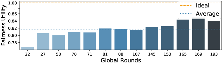
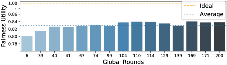
We illustrate the aspect of fairness in Fig. 5, which is defined by Def. 4. In line with our analysis, fairness improves slightly over time but remains low in the presence of Mavericks. Concretely, the system-wide fairness increases from slightly below 0.8 to close to 0.85, with an ideal situation being 1.0. The result is consistent for both data sets.
A.4 Empirical Observation of Client Selection
We evaluate a simple selection protocol that knows the identity of the one Maverick in the system and always selects them as one of the clients. Our example evaluation uses Fashion-MNIST dataset, other corresponding settings in detail are involved in Section 5. The one Maverick owns class ‘Trouser’ exclusively. For each class to be trained on the same number of data points, the Maverick owns times as much data as the other clients. All clients have equal communication and computation resources. Our main metrics are the global accuracy and the accuracy on class ‘Trouser’, which depends solely on the Maverick. We provide upper and lower bounds on the performance by comparing our setting with an i.i.d. distribution over all classes (denoted by i.i.d.) and one over all classes without the Maverick class (denoted by mav-never), respectively. When including a Maverick, we use random selection (denoted by mav-random) to compare with the case when the Maverick is always selected (denoted by mav-always).
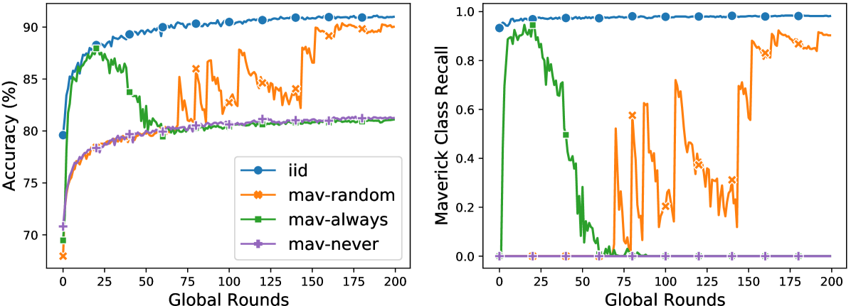
Fig. 6 indicates that while initially outperforming random selection and being similarly accurate as the upper bound of i.i.d. data distribution, always including a Maverick has a detrimental effect in the long run. The result can be explained as the inclusion of Mavericks enlarges the distance between the global distribution and the learned distribution. Concretely, the learned distribution is skewed towards the Maverick class as the majority of images it trains on is from the Maverick class, with the Maverick having more data than all other selected clients combined.
A.5 Design Support for FedEMD
Based on our insights from the previous experiment (See Sec A.4 in Supplement), we design FedEMD to involve Mavericks in the beginning but avoid overtraining by involving them less later on. In this manner, we achieve faster convergence and a light-weight protocol in comparison to Shapley Value. We utilize -convergence as the global round when the test accuracy reaches of the highest accuracy reached when using random selection. Here, we further assume that clients record their local data quantity per class to the federator. It has been shown that such reporting is indeed acceptable for privacy-preserving [3].
Three factors contributes to our selection method: i) Global distance, which is the distribution differences between single client and the aggregated global distribution of all clients. It indicates the differences from global distribution of each client and the one with higher global distance has high probability to be selected. ii) Current distance, which is the distance between the accumulated distribution over each rounds of the selected clients’ distribution and a single client. A larger current distance indicates that selecting the client might deter convergence, hence the probability of the client to be selected should be lower. iii) Round decay, which increases the impact of current distance over time to avoid non-convergence.
Hence, FedEMD considers both global and current distance on client data distribution to bias the selection strategy to involve Mavericks at the early stage with higher probability to increase convergence speed, while reducing the selection probability of Mavericks once the round decay becomes relevant to avoid skewing the distribution towards the Maverick classes. To measure the distance of distributions, the weight divergence [42] of and is:
| (20) | ||||
Note that is the Wasserstein Distance (EMD) of and the global distribution, which directly leads to the drift of by . Thus, we use Wasserstein Distance as the distance measure in our distribution-based FedEMD. The Wasserstein Distance is defined as:
| (21) |
where represents the set of all possible joint probability distributions of . represents the probability that appears in and appears in .
Additionally, compared with other popular distance measures, Wasserstein Distance is suitable in our case because: i) even if the support sets of the two distributions do not overlap or overlap very little, it still reflects the distance of two distributions, while the Jensen–Shannon Distance (JSD) [10] is constant in this case and the KLD approaches ; ii) it is more smooth in the sense that it avoids sudden changes in distance, in contrast to JSD.
A.6 Observation on the Impact of Mavericks
we first conduct experiments of learning a neural network classifier for Fashion-MNIST under scenarios of i.i.d. and in the presence of one Maverick owning all images of class ‘Trouser’. We study the convergence over the global rounds, considering four scenarios: i) random selection333The default client selection in FL is random policy. and i.i.d. distribution with equal quantity (i.i.d.-random), ii) Shapley Value-based selection and i.i.d. distribution with heterogeneous data quantity (size-het-svb), iii) random selection and one Maverick (maverick-random), and iv) Shapley Value-based selection and one Maverick (maverick-svb).
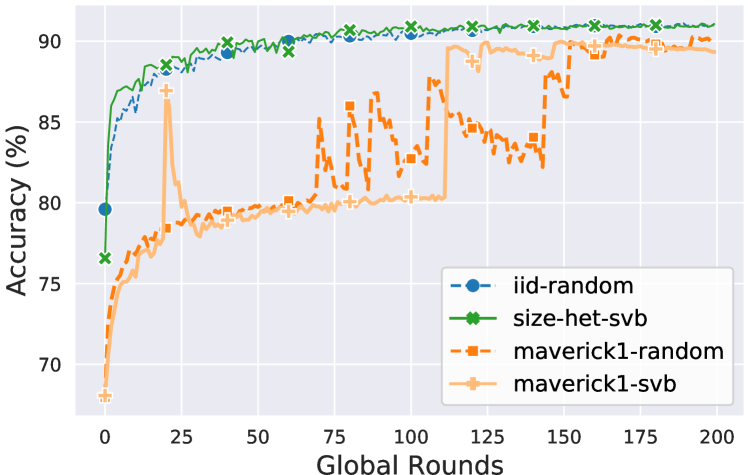
Figure 7 shows that random and Shapley Value-based selection both perform well in the scenarios that they are designed for. Yet, they both exhibit slow convergence for Mavericks, with Shapley Value not showing a clear advantage over the random selection. This result leads us to conjecture that Shapley Value is unable to fairly evaluate Mavericks’ contribution.
A.7 Computational Overhead of federator
| Algorithm | FedAvg | TiFL | FedFast | FedProx | FedEMD |
|---|---|---|---|---|---|
| Overhead | 1 | 2.4 | 1.76 | 1.56 | 1.04 |
Our overhead is measured by the computation time at the federator, see Table 2, with all experiments run on the same machine. We express the computation time relative to the baseline of random selection. On Fashion-MNIST dataset with FedAvg, the computation times for TiFL, FedFast, and FedEMD increase by a factor 2.4, 1.76, and 1.04. respectively, in comparison to random. As expected, FedEMD has the lowest overhead due to its light-weight design. TiFL and FedFast have notably higher overheads since TiFL performs expensive local model testing and FedFast performs K-means clustering for client selection each round and always choose Maverick whose training takes long. These results are consistent for all data sets, so we present only Fashion-MNIST due to space constraints.
A.8 Hardware and Software
We develop such a FL emulator via Pytorch and run experiments on Ubuntu 20.04, with 32 GB memory which is equipped with a GeForce RTX 2080 Ti GPU and a Intel i9 CPUs with 10 cores (2 threads each).
A.9 Details of the Datasets and Networks
The key characteristics of the datasets and corresponding neural networks are summarized in Table 3.
| Dataset | Type | Train | Classes | Test |
|---|---|---|---|---|
| MNIST | bilevel-28*28 | 60K | 10 | 10K |
| Fashion-MNIST | bilevel-28*28 | 60K | 10 | 10K |
| Cifar-10 | colored-28*28 | 50K | 10 | 10K |
| STL-10 | colored-96*96 | 5K | 10 | 8K |
MNIST: For the image classification of handwritten digits in MNIST, a very simple CNN with 2-convolutional layer followed by a densely-connected layer is used which is able to achieve accuracy of 99.5%. The output is a class label from 0-9. Fashion-MNIST: For the image classification of bilevel fashion related images in Fashion-MNIST, the neural network is the same as CNN in MNIST. Cifar-10: For this colored image classification task, the classes are completely mutually exclusive. Neural network applied is CNN with 6-convolutional layer and 2 densely-connected layer to map the output from 0-9. STL-10: This dataset consists of only 500 data in each class, in our federated setting, each non-Maverick owns 10 data in one label. It also use a shallow CNN with 3-convolutional layer followed by 2 fully-connected layer.
A.10 Recommend Parameters
-
•
MNIST: Batch size: 4; LR: 0.001; Momentum: 0.5; Scheduler step size: 50; Scheduler gamma: 0.1; : 0.15, 0.0015;
-
•
Fashion-MNIST: Batch size: 4; LR: 0.001; Momentum: 0.9; Scheduler step size: 10; Scheduler gamma: 0.1; : 0.15, 0.0015;
-
•
Cifar-10: Batch size: 10; LR: 0.01; Momentum: 0.5; Scheduler step size: 50; Scheduler gamma: 0.5; : 0.11, 0.0015;
-
•
STL-10: Batch size: 10; LR: 0.01; Momentum: 0.5; Scheduler step size: 50; Scheduler gamma: 0.5; : 0.11, 0.001;
Appendix B Broader Impact
Generalization and Limitations
We consider the contribution measurement and client selection in the presence of Mavericks, who hold large data quantities and exhibit skewed data distributions. When the number of exclusive Mavericks increases to the extreme (i.e. all over the clients are Mavericks), the Maverick scenario approaches the data heterogeneous scenarios considered in prior work [42]. When the number of shared Mavericks increases, the FL system approaches an i.i.d. scenario. In this paper, we do not consider differences in computational or network resources. We suggest to combine FedEMD with prior work [26, 15] to avoid selecting clients with insufficient resources.
Discrimination in Federated Learning
We have shown that Federated Learning discriminates against clients with unusual data both when assigning rewards and during the selection procedure. Note that this is in line with work on security enhancements for FL, which have also been shown to exclude users with diverse data [34]. Such a bias against clients with diverse data is likely to exclude people from minority groups from the learning process, as they can have data that is very specific to their experience as a member of a minority group. As a consequence, minority groups might be excluded from profiting from the learning outcome. Our difference enables to promote clients with diverse data strategically and is hence a first step to increasing diversity in Federated Learning. However, the profit of this step is limited, as long as security measures and lacking incentives are still likely to be biased against certain groups. More work is needed to ensure that Federated Learning does not amplify already existing social and institutional discrimination.