Is the black-widow pulsar PSR J1555–2908 in a hierarchical triple system?
Abstract
The Hz black-widow pulsar PSR J15552908, originally discovered in radio, is also a bright gamma-ray pulsar. Timing its pulsations using 12 yr of Fermi-LAT gamma-ray data reveals long-term variations in its spin frequency that are much larger than is observed from other millisecond pulsars. While this variability in the pulsar rotation rate could be intrinsic “timing noise”, here we consider an alternative explanation: the variations arise from the presence of a very-low-mass third object in a wide multi-year orbit around the neutron star and its low-mass companion. With current data, this hierarchical-triple-system model describes the pulsar’s rotation slightly more accurately than the best-fitting timing-noise model. Future observations will show if this alternative explanation is correct.
AAAA
1 Introduction
PSR J15552908, a neutron star spinning rapidly at Hz, resides in a tight hr binary system (Ray et al. 2022, submitted, hereafter Paper I) with a low-mass () companion (Kennedy et al. 2022, submitted). This millisecond pulsar (MSP) was first detected in a Green Bank Telescope (GBT) pulsar survey which targeted steep-spectrum radio sources (Frail et al., 2018) within the localization region of Fermi-Large Area Telescope (LAT; Atwood et al., 2009) gamma-ray sources. After the radio discovery, gamma-ray pulsations were detected, allowing the timing measurement of the system parameters over the -yr Fermi mission time span.
Timing analysis using the Large Area Telescope (LAT) data reveals variations of the spin frequency which are larger than is typical for MSPs (Kerr et al., 2015). Such variations are often seen in young gamma-ray pulsars, where they are labeled as “timing noise”. Timing noise is also present in MSP, but its weaker amplitude (Shannon & Cordes, 2010) is typically not detectable with the LAT (Kerr et al. 2022, submitted). Instead, the intrinsic rotational phase is generally well described by a quadratic function of time, i.e. a constant spin-down rate , with no detectable noise components above the measurement uncertainty. In contrast, for PSR J15552908 four additional terms in the rotational phase model are required.111In a gamma-ray timing analysis, timing noise is easily distinctive from the variations of the orbital period which are often seen in “spider” pulsars. While both variations happen on multi-year timescales, spin-frequency variations manifest as pulse phase drift, and variations of the short ( d) orbital period smear the pulse profile out.
Such strong variations suggest an alternative explanation. For example, in the case of the millisecond pulsar PSR J10240719, long thought to be isolated, the measurement of additional higher-order spin-frequency derivatives led to the conclusion that the pulsar could be in a very-long-period ( kyr) orbit with a low-mass companion (Kaplan et al., 2016).
In this paper, we discuss a similar alternative to the timing noise explanation for PSR J15552908: that the variations arise from the presence of a third body in the system. This additional object is in a wide, multi-year orbit around the closely orbiting neutron star and its low-mass companion. An extreme example of such a system would be the hierarchical-triple-system pulsar PSR J03371715 (Ransom et al., 2014).
With the currently available data, this model describes the pulsar as well as the timing-noise model, but provides a simple and clear physical explanation for the spin frequency variations.
2 Rotational phase model
To precisely track the rotational phase, the photon arrival times need to be corrected for the line-of-sight motion of the pulsar, if it is in an orbit with one or more companions. For a simple hierarchical triple system (HTS), we assume that the gravitational interaction between the two companions can be neglected, and the third body orbits the center of mass of the inner binary system. The photon times, corrected for the pulsar’s motion around the barycenter of the triple system, , can be expressed as a function of the photon’s emission time, , as
| (1) |
Here, and are the times light needs to travel the semimajor axis of the pulsar’s orbit due to the inner (i) and outer (o) companion projected onto the line of sight. and are dimensionless functions that describe the respective modulations depending on the orbital phases, and . The orbital angular frequencies and are defined by the orbital periods and via and .
Following Edwards et al. (2006), we can make a function of by Taylor expansion. To second order (i.e. including terms of order , , , and ), we find
| (2) | ||||
where and denote the first and second derivative of with respect to . For wide, multi-year outer orbits of low-mass companions, , so we neglect terms multiplied by this quantity, i.e. and .
In the case of a circular orbit, takes the simple form of a sinusoid, , with time of ascending node . Hence, and . Eq. (2) can also be applied to the widely used small-eccentricity-orbit “ELL1 model” (Lange et al., 2001), or the larger-eccentricity models presented in Nieder et al. (2020).
For the outer companion’s orbit of PSR J15552908, we use the full “BT model”, with eccentricity , and angle of periastron (Blandford & Teukolsky, 1976). is defined via and is computed numerically. Instead of using the parameter set , which is degenerate for small eccentricities, we use , , and (Lange et al., 2001).
In Section 3, we show that PSR J15552908 can be well described as an HTS with the inner orbit being circular and the outer orbit being eccentric.
For a timing analysis, it is helpful to have a good starting point in the multi-dimensional parameter space. The parameters describing the potential outer orbit can be roughly estimated from the timing solution presented in Paper I, which requires four additional frequency derivatives (“FX model”).
First, we need to derive how the observed frequency changes in the case of an outer circular orbit. Assuming only a non-zero spin frequency and a non-zero first time-derivative , the additional evolution of the spin frequency over time can be written in two ways:
| (3) | ||||
| (4) | ||||
Here, we denote the th frequency derivative as , and use an asterisk to indicate parameters measured with the FX model, and as well as . denotes the chosen reference time.
Second, since all parameters in Eq. (3) are measured, we fit Eq. (4) to Eq. (3) over the valid time span of the pulsar timing solution. To do this, we used curve_fit from scipy. This gives initial values for the five free parameters from Eq. (4).
From the fitted values, we find the inner binary barycenter’s potential movement would have a radius of a few tens of kilometers with an orbital period of yr, indicating a low-mass companion in a wide orbit.
3 Gamma-ray timing analysis
In our timing analysis, we use the LAT data prepared for the timing in Paper I. These data included P8R3 SOURCE-class photons (Atwood et al., 2013; Bruel et al., 2018) detected by LAT between 2008 August 03 and 2020 August 05 within a region of interest (RoI) around the pulsar position, with energies greater than MeV, and with a maximum zenith angle of .
The timing analysis is done twice, very similarly to the approach in Paper I. Firstly, we refit all the parameters of the FX model, i.e. we did not fix any parameters to the radio timing solution. Secondly, we amended the timing code with the HTS model given in Equations (1) and (2). To judge the timing results, we used the statistic (de Jager et al., 1989; Kerr, 2011) with the photon probability weights optimized following Bruel (2019), the likelihood (Abdo et al., 2013), and the Bayesian Information Criterion (BIC; Schwarz, 1978). The latter is based on the likelihood but with a penalty factor proportional to the degrees of freedom to penalize higher-dimensional models.
In the timing analysis, we tried to find the parameters that maximize for a given model. In the case of the HTS model, we tested the circular and eccentric options, where the latter requires two additional parameters. The eccentric orbit model is favored by all three statistics. For the FX model, we added spin-frequency derivatives until the test statistics and stopped improving significantly, which is in turn disfavored by the Bayesian Information Criterion (BIC). Here, adding six additional derivatives in principle leads to and values of a similar size to the HTS model. However, the last model favored by the BIC is the one with four additional frequency derivatives. The final timing solutions for the FX and HTS models are reported in Table 1.
In the timing analysis with the HTS model, the highest test statistics are found for an eccentric () outer orbit of d. With the LAT data span being only slightly shorter, the spin parameters and are still correlated with the outer-orbit Keplerian parameters , and . However, this covariance is small enough to not pose a problem for the timing analysis. Note, that the timing analysis does not give any information on the inclination between the orbits as only the line-of-sight motion can be measured.
The highest test statistics, and , seem to favor the HTS model over the FX model (see Table 1). Since each model has a different number of free parameters, we invoke the BIC. The BIC’s penalty for the additional parameter removes most of the advantage the HTS model had. However, the BIC still slightly favors the HTS model over the FX model (). Our final timing solutions over years of LAT data using the FX model and the HTS model are shown in Table 1.
In order to more directly compare the timing noise to that of other MSPs, we have analyzed it by following the methods of Lentati et al. (2014), adapted to gamma-ray data as in Kerr et al. (2022, submitted). In this approach, the timing noise is assumed to originate in a stationary process, thus having a unique description with a power spectral density which we assume to follow a power law, . The timing model parameters, timing noise parameters and , and the Fourier coefficients of the timing noise process are all determined jointly by maximizing the likelihood, which includes a Gaussian component that constrains the Fourier coefficients to follow the specified power law. We estimate uncertainties on the timing noise parameters from the curvature of the likelihood at its maximum value, and obtain and spectral index .
| Parameter | FX value | HTS value |
|---|---|---|
| Range of observational data (MJD) | – | |
| Reference epoch (MJD) | ||
| Statistics | ||
| statistic | ||
| Log-Likelihood | ||
| BIC | ||
| Timing parameters | ||
| R.A., (J2000.0) | ||
| Decl., (J2000.0) | ||
| Spin frequency, (Hz) | ||
| 1st spin-frequency derivative, (Hz s-1) | ||
| 2nd spin-frequency derivative, (Hz s-2) | ||
| 3rd spin-frequency derivative, (Hz s-3) | ||
| 4th spin-frequency derivative, (Hz s-4) | ||
| 5th spin-frequency derivative, (Hz s-5) | ||
| Inner-orbit binary parameters | ||
| Proj. semimajor axis, (lt-s) | ||
| Orbital period, (days) | ||
| Epoch of ascending node, (MJD) | ||
| Outer-orbit binary parameters | ||
| Proj. semimajor axis, (lt-s) | ||
| Orbital period, (days) | ||
| Epoch of ascending node, (MJD) | ||
| 1st Laplace-Lagrange parameter, | ||
| 2nd Laplace-Lagrange parameter, | ||
Note. — Numbers in parentheses are statistical uncertainties on the final digits. The JPL DE405 solar system ephemeris has been used, and times refer to TDB.
4 Discussion
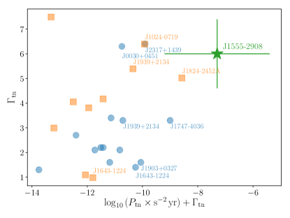
The spin-frequency variations of PSR J15552908 (see also Paper I) are unusually large in amplitude for the timing noise of an MSP (Kerr et al., 2015). Indeed, Figure 1 shows the timing noise spectral properties for two samples of MSPs as measured by the pulsar timing arrays NANOGrav (Arzoumanian et al., 2020) and the PPTA (Goncharov et al., 2021), along with our measured values for PSR J15552908. It is possible this collection of timing noise measurements is biased by selection for inclusion in a Pulsar Timing Array (PTA). However, the driving concern for inclusion is radio brightness, and often timing noise emerges only after many years of observation. Consequently, we expect such a bias to be modest. The abscissa in Figure 1 is defined in such a way to indicate the timing noise at frequency , i.e. a time scale comparable to the length of the data set. PSR J15552908 is a clear outlier, with more than times the timing noise amplitude of the next strongest pulsar, J18242452A in the M28 globular cluster, whose timing noise presumably includes contributions from the cluster potential and close passages by other cluster members. Another noteworthy example is PSR J19392134, an isolated MSP considered to be a “noisy” timer for which Shannon et al. (2013) invoked an asteroid belt surrounding the pulsar to explain the observed timing variations, but which has a timing noise amplitude that is times weaker than that of PSR J15552908.
In this work we have presented an alternative explanation, in which another companion orbits the inner binary system, a hierarchical triple system. To account for the additional body in the system, we have developed a simple, but sufficient rotational phase model. In a timing analysis with current data, the results with both models are indistinguishable. Within the timing range the maximum phase offset between both models is of one rotation.
It is predictable that the two models would not differ much. The variations are measurable with the LAT data, but the peak-to-peak amplitude of the phase offset is still only of one rotation. Furthermore, the potential outer companion would have completed roughly one orbit during the Fermi mission which can be well approximated with the six spin parameters of the FX model.
In the following, we will make estimates of the companion mass and the orbital radius, but want to note that these directly depend on the outer orbital period . Due to the strong correlations between the orbital parameters (see Section 3), these estimates should be treated with caution and will only give an order of magnitude.
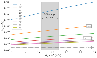
The binary mass function may be used to estimate the mass of the outer companion (see Fig. 2). For common pulsar masses , an inner companion mass (Kennedy et al. 2022, submitted), and inclination angles , the outer companion would have roughly a Mercury-like mass . To date, this companion would still be listed among the four lowest-mass extrasolar planets222http://exoplanet.eu/catalog/.
A comparably low-mass () companion has also been found for a planet orbiting PSR B125712 (Wolszczan, 1994), the pulsar thanks to which, years ago, the first extrasolar planetary companions have been identified (Wolszczan & Frail, 1992). However, unlike the periods of the planets orbiting PSR B125712 with tens to hundreds of days, the probable companion of PSR J15552908 takes considerably longer with days.
The putative triple system of PSR J15552908 is extremely hierarchical. The pulsar’s mass is times larger than the inner companion’s mass, and even times larger than the outer companion’s mass. The ratio between outer and inner orbital period is . Using Kepler’s third equation, the masses from optical modeling, and the timing parameters one can estimate the semimajor axis of the inner companion’s orbit as lt-s and the outer companion’s orbit as lt-s. Systems with such extreme hierarchical properties are typically assumed to be stable on long timescales (Georgakarakos, 2008).
Other HTSs which include a pulsar are known. PSR J03371715 is in an orbit with two white dwarf companions (Ransom et al., 2014). Carefully studying this system led to one of the most stringent tests of General Relativity’s predicted universality of free fall (Archibald et al., 2018; Voisin et al., 2020). A binary system consisting of the MSP PSR B162020 and a white dwarf is orbited by a planetary companion of (Thorsett et al., 1993; Sigurdsson et al., 2003).
An open question is how such a system could have formed. A pulsar planet can form in various ways (see, e.g., Podsiadlowski, 1993). Since PSR J15552908 is not in a dense Globular Cluster, it seems unlikely that the triple was formed in an exchange interaction between systems as is suggested for PSR B162020 (Sigurdsson et al., 2003). Another option could be that the inner binary captured a free-floating planet (see, e.g., Miret-Roig et al., 2021). On the other hand, the planet might have formed from a circumbinary debris disk (see, e.g., Pelupessy & Portegies Zwart, 2013), in which case it would be expected that the orbits are coplanar.
Only to emphasize the power of pulsar timing with LAT data, we want to note that if PSR J15552908 has an additional planetary-mass companion, then it was discovered because over the course of billion pulsar rotations, the phase drifted by of one single rotation.
So, is PSR J15552908 in a hierarchical triple system? We do not know, yet. With current data, both of the timing models that are presented here track the pulsar’s rotation equally well. However, the ongoing Fermi mission will continue to collect data, and eventually the nature of this system will be resolved.
References
- Abdo et al. (2013) Abdo, A. A., Ajello, M., Allafort, A., et al. 2013, ApJS, 208, 17, doi: 10.1088/0067-0049/208/2/17
- Archibald et al. (2018) Archibald, A. M., Gusinskaia, N. V., Hessels, J. W. T., et al. 2018, Nature, 559, 73, doi: 10.1038/s41586-018-0265-1
- Arzoumanian et al. (2020) Arzoumanian, Z., Baker, P. T., Blumer, H., et al. 2020, ApJ, 905, L34, doi: 10.3847/2041-8213/abd401
- Atwood et al. (2013) Atwood, W., Albert, A., Baldini, L., et al. 2013, ArXiv e-prints. https://arxiv.org/abs/1303.3514
- Atwood et al. (2009) Atwood, W. B., Abdo, A. A., Ackermann, M., et al. 2009, ApJ, 697, 1071, doi: 10.1088/0004-637X/697/2/1071
- Blandford & Teukolsky (1976) Blandford, R., & Teukolsky, S. A. 1976, ApJ, 205, 580, doi: 10.1086/154315
- Bruel (2019) Bruel, P. 2019, A&A, 622, A108, doi: 10.1051/0004-6361/201834555
- Bruel et al. (2018) Bruel, P., Burnett, T. H., Digel, S. W., et al. 2018, arXiv e-prints. https://arxiv.org/abs/1810.11394
- de Jager et al. (1989) de Jager, O. C., Raubenheimer, B. C., & Swanepoel, J. W. H. 1989, A&A, 221, 180
- Edwards et al. (2006) Edwards, R. T., Hobbs, G. B., & Manchester, R. N. 2006, MNRAS, 372, 1549, doi: 10.1111/j.1365-2966.2006.10870.x
- Frail et al. (2018) Frail, D. A., Ray, P. S., Mooley, K. P., et al. 2018, MNRAS, 475, 942, doi: 10.1093/mnras/stx3281
- Georgakarakos (2008) Georgakarakos, N. 2008, Celestial Mechanics and Dynamical Astronomy, 100, 151, doi: 10.1007/s10569-007-9109-2
- Goncharov et al. (2021) Goncharov, B., Reardon, D. J., Shannon, R. M., et al. 2021, MNRAS, 502, 478, doi: 10.1093/mnras/staa3411
- Kaplan et al. (2016) Kaplan, D. L., Kupfer, T., Nice, D. J., et al. 2016, ApJ, 826, 86, doi: 10.3847/0004-637X/826/1/86
- Kerr (2011) Kerr, M. 2011, ApJ, 732, 38, doi: 10.1088/0004-637X/732/1/38
- Kerr et al. (2015) Kerr, M., Ray, P. S., Johnston, S., Shannon, R. M., & Camilo, F. 2015, ApJ, 814, 128, doi: 10.1088/0004-637X/814/2/128
- Lange et al. (2001) Lange, C., Camilo, F., Wex, N., et al. 2001, MNRAS, 326, 274, doi: 10.1046/j.1365-8711.2001.04606.x
- Lentati et al. (2014) Lentati, L., Alexander, P., Hobson, M. P., et al. 2014, MNRAS, 437, 3004, doi: 10.1093/mnras/stt2122
- Miret-Roig et al. (2021) Miret-Roig, N., Bouy, H., Raymond, S. N., et al. 2021, Nature Astronomy, doi: 10.1038/s41550-021-01513-x
- Nieder et al. (2020) Nieder, L., Allen, B., Clark, C. J., & Pletsch, H. J. 2020, ApJ, 901, 156, doi: 10.3847/1538-4357/abaf53
- Pelupessy & Portegies Zwart (2013) Pelupessy, F. I., & Portegies Zwart, S. 2013, MNRAS, 429, 895, doi: 10.1093/mnras/sts461
- Podsiadlowski (1993) Podsiadlowski, P. 1993, in Astronomical Society of the Pacific Conference Series, Vol. 36, Planets Around Pulsars, ed. J. A. Phillips, S. E. Thorsett, & S. R. Kulkarni, 149–165
- Ransom et al. (2014) Ransom, S. M., Stairs, I. H., Archibald, A. M., et al. 2014, Nature, 505, 520, doi: 10.1038/nature12917
- Schwarz (1978) Schwarz, G. 1978, Annals of Statistics, 6, 461
- Shannon & Cordes (2010) Shannon, R. M., & Cordes, J. M. 2010, ApJ, 725, 1607, doi: 10.1088/0004-637X/725/2/1607
- Shannon et al. (2013) Shannon, R. M., Cordes, J. M., Metcalfe, T. S., et al. 2013, ApJ, 766, 5, doi: 10.1088/0004-637X/766/1/5
- Sigurdsson et al. (2003) Sigurdsson, S., Richer, H. B., Hansen, B. M., Stairs, I. H., & Thorsett, S. E. 2003, Science, 301, 193, doi: 10.1126/science.1086326
- Thorsett et al. (1993) Thorsett, S. E., Arzoumanian, Z., & Taylor, J. H. 1993, ApJ, 412, L33, doi: 10.1086/186933
- Voisin et al. (2020) Voisin, G., Cognard, I., Freire, P. C. C., et al. 2020, A&A, 638, A24, doi: 10.1051/0004-6361/202038104
- Wolszczan (1994) Wolszczan, A. 1994, Science, 264, 538, doi: 10.1126/science.264.5158.538
- Wolszczan & Frail (1992) Wolszczan, A., & Frail, D. A. 1992, Nature, 355, 145, doi: 10.1038/355145a0