Is there a one-to-one correspondence between interparticle interactions and physical properties of liquid?

Let us assume that for an investigated many-particle homogeneous isotropic system, such as a liquid or an amorphous solid, structural data are initially known, and these structural data are specified by the radial distribution function $g(r)$ of particles. The system under study can be a real physical system or a model system, where the interaction of particles is specified by a certain potential $u(r)$. Consequently, the structural data can be experimental or calculated based on the results of molecular dynamics simulations or Monte Carlo simulations with a given potential. The radial distribution function corresponding to these structural data is known. This function has the meaning of an input quantity in the given problem and will be denoted as $g_{\text{obj}}(r)$, where the subscript obj means objective.

Further, our goal is to recover the potential of interparticle interaction $u(r)$. Let us assume that it belongs to the family of the potentials $\overline{u}_{\mathbf{p}}(r)$, i.e.

$$u(r)\in\overline{u}_{\mathbf{p}}(r),$$

the analytical form of which are specified by the set of parameters

$$\mathbf{p}=\{p_{1},p_{2},\ldots,p_{n}\},\quad n\in\mathcal{N}.$$

(1)

The values of the parameters $\{p_{1},p_{2},\ldots,p_{n}\}$ are initially unknown. However, some general form of the potential $u_{\mathbf{p}}(r)$ can be chosen taking into account the nature of the many-particle system. So, for example, it could be a system of point charges (electrons, ions), a system of dipoles or colloid particles, etc. Then, the parameters $\{p_{1},p_{2},\ldots,p_{n}\}$ can be the exponents in attractive or repulsive contributions, the weights of these contributions, the characteristics of selected directions in particle interactions in the case of nonspherical potentials, etc. Thus, the problem of recovering the potential is reduced to determining the values of these parameters at which the model potential $u_{\mathbf{p}}(r)$ will correctly reproduce the structure of the system, namely, the ‘experimental’ radial distribution function $g_{\text{obj}}(r)$.

The exact relationship between the interaction potential $u(r)$ and the distribution function $g_{\text{obj}}(r)$ is known only for the case of a rarefied gas [43, 44, 45]:

$$g_{\text{obj}}(r)=\exp\left[-\frac{u(r)}{k_{\text{B}}T}\right].$$

(2)

For the condensed phases such as a high-dense gas, liquid and amorphous solid, a correspondence between the quantities $g(r)$ and $u(r)$ is unknown, and it is not possible to calculate analytically the interaction potential $u(r)$ on the basis of the known function $g_{\text{obj}}(r)$. On the other hand, the radial distribution function $g(r)$ itself can be accurately calculated using configuration data resulted from molecular dynamics or Monte-Carlo simulations, if the potential $u(r)$ is specified for a given thermodynamic state of the system under study [46, 47]. Thus, to restore the potential, we can use the following computational procedure. It is necessary to try different modifications of the potential $u_{\mathbf{p}}(r)$ for molecular dynamics (or Monte-Carlo) simulations, determining the radial distribution function $g(r)$ and each time comparing the obtained trial function $g(r)$ with the objective function $g_{\text{obj}}(r)$. The procedure should be carried out until the required correspondence between functions $g(r)$ and $g_{\text{obj}}(r)$ is obtained. Note that a modification of the potential is actually determined by values of the parameters $\{p_{1},p_{2},\ldots,p_{n}\}$. Thus, in order to restore the potential in accordance with this procedure, we really need to sort out various combinations of the values of its parameters $\{p_{1},p_{2},\ldots,p_{n}\}$ and find the optimal one.

Let us choose the quantity $R(\mathbf{p})$ determined by the following relation

$$R(\mathbf{p})=\frac{1}{\mathcal{N}}\sum_{i=1}^{\mathcal{N}}\left[g_{\text{obj}}(r_{i})-g_{\mathbf{p}}(r_{i})\right]^{2},$$

(3)

as a measure of similarity (or difference) between the trial function $g(r)$ and the objective function $g_{\text{obj}}(r)$. Here, $\mathcal{N}$ is the number of segments in $r$-axis, and $i$ is the label of a segment. In fact, the quantity $R(\mathbf{p})$ is the so-called mean squared deviation or weighted residual sum of squares known in statistics [48], and it can only take non-negative values. If $R(\mathbf{p})=0$, then both the functions $g(r)$ and $g_{\text{obj}}(r)$ coincide. The more these functions differ, the greater value the quantity $R(\mathbf{p})$ takes.

Further, let us introduce a phase space formed by the set of parameters $\mathbf{p}$. Hypothetically, each model potential from the family $\overline{u}_{\mathbf{p}}(r)$ can be associated with a value of the quantity $R(\mathbf{p})$. The set of resulting values of the quantity $R(\mathbf{p})$ will yield a landscape (surface) in this phase space. Then, the location of the global minimum of this landscape, where the quantity $R(\mathbf{p})$ tends to zero, should be directly associated with the values of the parameters $\{p_{1},p_{2},\ldots,p_{n}\}$ of the sought model potential $u(r)$. Finding this global minimum in the landscape is the same as finding the potential $u(r)$, which is capable to reproduce the experimental structure characteristic $g_{\text{obj}}(r)$ with a required accuracy. Thus, we have the typical optimization problem that can be solved by means of the differential evolution algorithm [34].

The first step of the proposed computational scheme is to determine the family of model potentials, within which the search for the required model will be carried out. First of all, it is necessary to define some general model $\overline{u}_{\mathbf{p}}(r)$, the free parameters $\mathbf{p}$ that set the model $\overline{u}_{\mathbf{p}}(r)$, as well as the range of acceptable values of these parameters. An important point is the number of free parameters $\mathbf{p}$ and the range of their acceptable values. A relatively small number of parameters with narrow ranges of acceptable values simplifies the optimization process and increases the chances of achieving convergence of the values of free parameters with limited computing resources. On the other hand, a larger number of parameters significantly increases a flexibility of parameterization and increases the chances of finding a solution.

The differential evolution algorithm as applied to the problem of potential recovering includes two computing procedures.

The first procedure is associated with finding the equilibrium configurations of many-particle system in a given thermodynamic state. These configurations should be generated using the test model potential of interparticle interaction. They will be required for the subsequent calculation of the radial distribution function $g(r)$ and comparison with the objective function $g_{\text{obj}}(r)$. Consequently, it is convenient here to use a computational program or package that supports molecular dynamics or Monte-Carlo simulations. For example, this could be the LAMMPS package [49], which implements molecular dynamics simulations and is distinguished by high computational speed. It supports for calculations on GPU, simulations in various statistical ensembles ($NVE$, $NVT$, $NpT$), as well as on-the-fly calculations of various structural and transport properties.

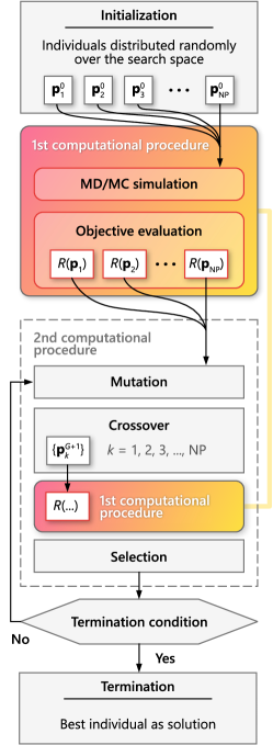
The second procedure involves computations in the framework of the adapted differential evolution algorithm, the main elements of which are given in Fig. 1. In accordance with the standard terminology of evolutionary algorithms, one can say that this computational procedure involves the following: formation of generations of individuals, as well as operations of mutation, crossover and selection of individuals [50]. So, let us define these basic terms and operations of the differential evolutionary algorithm methodology.

By individual, we mean a model potential $u_{\mathbf{p}_{i}}(r)$ from the initially given family of potentials $\overline{u}_{\mathbf{p}}(r)$. Here, $i$ is the label of an individual with a unique genome $\mathbf{p}_{i}$, which is a set of the parameters with specific numerical values, i.e.

$$\mathbf{p}_{i}=\{p_{1}^{(i)},p_{2}^{(i)},\ldots,p_{n}^{(i)}\}.$$

Thus, $p_{n}^{(i)}$ has the meaning of a gene. From mathematical point of view, the genome $\mathbf{p}_{i}$ can be viewed as a vector with components $p_{1}^{(i)}$, $p_{2}^{(i)}$, $\ldots$, $p_{n}^{(i)}$. Therefore, all the standard mathematical operations with vectors are also applicable to it. Then, the quantity $n$ has the meaning of the dimensionality of the search space. A set of individuals form a population of a certain generation $G$; and the population size is denoted as $NP$. The size of the population is determined by the dimensionality of the search space $n$ [34]. As was found earlier (see, for example, work [34], p. 356), there is a rule of thumb which establishes a quantitative correspondence between the dimensionality of the search space $n$ and the minimum number of individuals in the population $NP$:

$$NP=(5\div 10)\,n\,.$$

(4)

The minimal permissible value of $NP$ is 4. We note that the term generation is, in a sense, a characteristic of a population: thus, there may be a population of a parent or a child generation. Therefore, in some cases it is convenient and appropriate to use the term generation instead of population. Individuals of each generation undergo operations of mutation, crossover and selection.

Mutation. – Mutation is defined as the mathematical operation applied to three random genomes $\mathbf{p}_{k}^{G}$, $\mathbf{p}_{l}^{G}$ and $\mathbf{p}_{m}^{G}$ of the individuals of the same population $G$ in accordance with the following vector addition rule:

$$\mathbf{p}_{k}^{\widetilde{G}+1}=\mathbf{p}_{k}^{G}+F\left(\mathbf{p}_{l}^{G}-\mathbf{p}_{m}^{G}\right).$$

(5)

Here, the weight coefficient $F$ known also as the mutation factor can take some a chosen non-integer value from the range $[0,2]$ as indicated in Ref. [51]. The higher value of $F$, the more perturbations/changes are introduced into the genome. As found in Ref. [34], values of $F$ smaller than 0.4 or larger than 1 are effective only in specific cases. This operation is applied to the genomes of all the individuals of the population $G$. The operation is considered acceptable if the obtained values of the genome parameters $\mathbf{p}_{k}$ of the individual $u_{\mathbf{p}_{k}}(r)$ of the new mutated generation $(\widetilde{G}+1)$ do not go beyond the range of permissible values. Such an implementation of mutation was proposed in the original work on differential evolution and it is essentially a reproduction of a similar operation in the Nelder-Mead method [51] (see, for example, Eq. (1.25) in [51]). It should be noted that to improve population diversity, the mutation operation given by equation (5) can be modified so as to be performed at a time on a larger number of individuals, if the population size $NP$ is large enough [52].

Crossover. – Crossover is the operation carried out with the genomes of a pair of individuals, one each from the parental $G$ and the new mutated $(\widetilde{G}+1)$ generations. Let us show this operation by the example of the formation of the $i$-th individual for the new generation $(G+1)$:

$$p_{n}^{G+1}=\begin{cases}p_{n}^{\widetilde{G}+1}&\text{if $\xi\leqslant C_{R}$ or $n=n_{\text{rand}}$\,,}\\ p_{n}^{G}&\text{otherwise.}\end{cases}$$

(6)

Here, $\xi$ is a random non-integer number from $[0,1)$. All the individuals of both the generations $G$ and $(\widetilde{G}+1)$ must undergo this operation. Eq. (6) sets that all the components of a vector $\mathbf{p}_{k}^{G}$ of the parental generation $G$ are replaced with a certain probability $C_{R}$ by the components of the new mutated vector $\mathbf{p}_{k}^{\widetilde{G}+1}$, while a one component, chosen at random and with the label $n_{\text{rand}}$, is necessarily replaced by the corresponding component of the mutated vector. The quantity $C_{R}$ is referred to as the crossover rate and can take a non-integer value from the range $[0,1]$. Sequential application of mutation and crossover operations ensures that all the individuals of the new generation $(G+1)$ will be distinct from the individuals of the parent generation $G$. The greater the value of $C_{R}$, the more substantial is the change in the individuals. Solving the problem of restoring potential is computationally challenging, so rapid evolution of generations is necessary. Therefore, it is reasonable to set large values of $C_{R}$, close to 1.

Selection. — The last stage, as a result of which the child generation is finally formed, is associated with the selection operation. The selection operation must ensure the evolution of generations in a required direction. Consequently, those individuals should be selected whose characteristics are closest to the required ones. In the problem under consideration, selection is carried out on the basis of a parameter $R(\mathbf{p}_{j})$ determined for each $j$th individual [see Eq. (3)]. The evolution should lead to the individuals with the lowest values of the parameter $R$, which, in the methodology of evolutionary algorithms, has a meaning of a fitness function or cost function [51]. To perform the selection operation, it is necessary to consider once again the pairs of individuals, one for the parental $G$-generation and for the $(G+1)$-generation obtained as a result of mutations and crossovers. For the child generation, an individual is selected from these two, for which the cost function $R$ takes the smallest value.

Flowchart of the adapted differential evolution algorithm is given in Fig. 1. The initial population, i.e. the zero generation population, is created by selecting random individuals in the phase space (search space). Note that the probabilities of choosing one or another individual are the same. This is followed by the first computational procedure associated with finding equilibrium configurations for individuals in a given generation. Here, for all the individuals, the cost function $R$ is calculated. After that, the condition for termination of the computational algorithm is checked. If the condition is not met, then there is a transition to the second computing procedure with the simulation of the evolution process and a subsequent return to the first computing procedure. The algorithm is performed until an individual with the required properties is found.

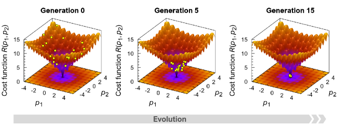
In fact, this algorithm should implement the search for the global minimum of the landscape $R(\mathbf{p})$. The more complex the geometry of the landscape $R(\mathbf{p})$, the more difficult it is to carry out such a search. Fig. 2 shows the results of testing the adapted differential evolution algorithm as applied to finding the global minimum of the model surface given by the Ackley function [53]. Notice that the Ackley function is a non-convex function containing many local minima, and it is usually used to test performance for optimization algorithms. In our test case, we define the cost function $R(\mathbf{p})$ as the Ackley function of two variables $p_{1}$ and $p_{2}$:

	$\displaystyle R(p_{1},p_{2})$	$\displaystyle=$	$\displaystyle-20\exp\left[-\frac{1}{5}\sqrt{\frac{\left(p_{1}^{2}+p_{2}^{2}\right)}{2}}\right]$
			$\displaystyle-\exp\left[\frac{\cos{2\pi}p_{1}+\cos{2\pi}p_{2}}{2}\right]+e+20\,,$

which has the global minimum

$$R(0,\,0)=0\,.$$

In Eq. (2.2), $e$ is the Euler’s number, and all the numerical coefficients are the same as in the original work [53]. As seen in Fig. 2, the fifteenth generation population converges at the point $R(0,\,0)=0$, indicating that the adapted differential evolution algorithm successfully finds the global minimum. Note that the algorithm was performed for a population of the size $NP=20$. Following the results of Ref. [54], the mutation factor $F$ and crossover rate $C_{R}$ were taken to be $0.44$ and $0.88$, respectively.

Let us check the efficiency of the above method for the problem of restoring the Lennard-Jones potential

$$u_{\text{LJ}}(r)=4\epsilon\left[\left(\frac{\sigma}{r}\right)^{p_{1}}-\left(\frac{\sigma}{r}\right)^{p_{2}}\right]$$

(8)

$$\mathrm{with}\quad p_{1}=12\quad\mathrm{and}\quad p_{2}=6$$

from the known radial distribution function $g(r)$ for some thermodynamic ($\rho,\,T$)-state. Here, $\epsilon$ and $\sigma$ are the characteristic scales of energy and length given by the potential; and, throughout the section, all physical quantities will be defined in terms of these characteristics.

The Lennard-Jones potential is a special case of the Mie potential [55], which is a linear combination of repulsive and attractive contributions with arbitrary power dependencies:

$$\overline{u}_{p_{1},p_{2}}(r)=\frac{p_{1}}{p_{1}-p_{2}}\left(\frac{p_{1}}{p_{2}}\right)^{\frac{p_{2}}{p_{1}-p_{2}}}\epsilon\left[\left(\frac{\sigma}{r}\right)^{p_{1}}-\left(\frac{\sigma}{r}\right)^{p_{2}}\right]$$

(9)

$$\mathrm{with}\quad p_{1},p_{2}>0,$$

and

$$u_{\text{LJ}}(r)\in\overline{u}_{p_{1},p_{2}}(r).$$

The concrete analytic form of the Mie potential is given by the pair of parameters $p_{1}$ and $p_{2}$. Thus, if the function $g(r)$ for the Lennard-Jones system is known, then the problem of restoring the Lennard-Jones potential naturally reduces to finding the numerical values of the parameters $p_{1}$ and $p_{2}$ of the Mie potential or to finding the point $R(p_{1},p_{2})$ corresponding to a global minimum on the landscape $\mathcal{R}^{2}$ formed by the parameters $p_{1}$ and $p_{2}$.

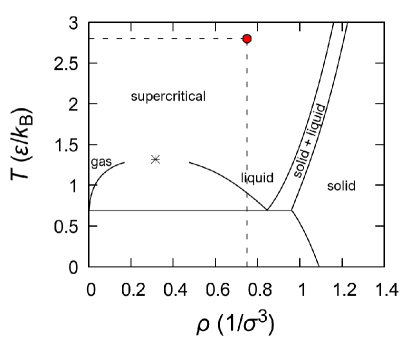
In the case of simple monatomic systems, such as the Lennard-Jones and/or Mie system, the thermodynamic states with the most complex homogeneous structure arise for the equilibrium liquid and supercritical fluid phases [56]. For this reason, in this study, we consider the state with the temperature $T=2.8\,\epsilon/k_{B}$ and the density $\rho=0.75\,\sigma^{-3}$, that corresponds for the case of the Lennard-Jones system to supercritical fluid at the pressure $p=6.6\,\epsilon/\sigma^{3}$. The ($\rho,\,T$) phase diagram of the Lennard-Jones system is given in Fig. 3. Note that for this isobar $p=6.6\,\epsilon/\sigma^{3}$ the melting temperature (liquidus) of the Lennard-Jones system is estimated to be $T_{m}\simeq 1.1\,\epsilon/k_{B}$, whereas the isotherm $T=2.8\,\epsilon/k_{B}$ intersects the melting line in the ($p,\,T$) phase diagram at the pressure $p_{m}\simeq 6.0\,\epsilon/\sigma^{3}$. Obviously, when the values of the parameters $p_{1}$ and $p_{2}$ of the Mie potential change from the values corresponding to the Lennard-Jones potential, the melting line in the phase diagram will also change.

For the chosen thermodynamic state of the Lennard-Jones fluid, the objective radial distribution function $g_{\text{obj}}(r)$ was preliminarily determined, which was subsequently used as an input quantity in the calculation procedures. The computational procedure related to the determination of the radial distribution function $g_{p_{1},p_{2}}(r)$ with the trial potential $u_{p_{1},p_{2}}(r)$ was performed in the framework of equilibrium molecular dynamics simulations in the $NpT$ ensemble. This ensemble is chosen for two reasons. First, such an ensemble makes it possible to realize conditions close to experimental ones, where temperature and pressure can be controlled. Second, molecular dynamics simulations in $NVE$ or $NVT$ ensembles with trial potentials can produce structurally heterogeneous systems (e.g., with pores and voids). In other words, no guarantee that any trial potential at $V,E=\mathrm{const}$ (or $V,T=\mathrm{const}$) conditions will produce the equation of state of the target system (namely, the equilibrium density of the target system). All simulations were performed for a cubic simulation box with $N=30\,000$ particles; and periodic boundary conditions were applied in all directions. The pressure was controlled by the Berendsen barostat [46]. To optimize the molecular dynamics simulations, we apply to the trial potential $u_{p_{1},p_{2}}(r)$ and the corresponding force $f_{p_{1},p_{2}}(r)$ the so-called shifted force technique given by the conditions [59]

	$$u^{\text{SF}}_{p_{1},p_{2}}(r)=\begin{cases}u_{p_{1},p_{2}}(r)-\left.(r-r_{c})\displaystyle{\frac{\partial}{\partial r}}u_{p_{1},p_{2}}(r)\right|_{r=r_{c}}\\ \\ \hskip 42.67912pt-u_{p_{1},p_{2}}(r_{c})&\hskip-51.21504pt\text{if }r\leq r_{c};\\ \\ 0&\hskip-51.21504pt\text{if }r>r_{c}\end{cases}$$		(10a)
and
	$$f^{\text{SF}}_{p_{1},p_{2}}(r)=\begin{cases}f_{p_{1},p_{2}}(r)-f_{p_{1},p_{2}}(r_{c})&\text{if }r\leq r_{c};\\ 0&\text{if }r>r_{c}\end{cases}$$		(10b)

with the cutoff distance chosen as $r_{c}=5.0\,\sigma$.

The search for the values of the Mie potential parameters that would be able to reproduce the radial distribution function of the Lennard-Jones liquid was carried out in the following ranges of parameter values:

$$p_{1}\in[10.0,15.0]\quad\text{and}\quad p_{2}\in[3.0,8.0],$$

(11)

where the parameters $p_{1}$ and $p_{2}$ are real numbers specified with an accuracy of five decimal place.

The first (main) maximum of the objective radial distribution function $g_{\text{obj}}(r)$ of the Lennard-Jones liquid is characterized by a shape close to Gaussian, which is typical for a system of particles interacting through the softcore potential. The exponent $p_{1}=15.0$ for the repulsion contribution taken as the largest in our considerations seems reasonable, since for larger values of $p_{1}$ this contribution will approach the hard-sphere potential. Further, the selected maximum value $p_{2}=8.0$ of the attractive contribution corresponds to the dipole-quadrupole interaction, which strongly depends on distance $r$. Nevertheless, it is necessary to note that the ranges for values of both the parameters $p_{1}$ and $p_{2}$ can be taken even larger than in (11).

Thus, the search for the potential is carried out on the basis of the known radial distribution function $g_{\text{obj}}(r)$. It is assumed that the temperature and density corresponding to this function are known. Trial potentials of interparticle interaction are generated on the basis of the Mie potential given by expression (9), where the parameters $p_{1}$ and $p_{2}$ can take values from the ranges defined by (11). Thus, the ranges given by (11) determine the specific region of the $\mathcal{R}^{2}$ space within which the point $R(p_{1},p_{2})$ will be searched.

Finally, it should be noted that the size of each population was sixty-four individuals (trial potentials), i.e. $NP=64$, that is optimal from point of view of the available computing resources. As in the case of the Ackley function considered above, the mutation rate $F$ and the crossover rate $C_{R}$ were taken equal to $0.44$ and $0.88$, respectively. These values of both the parameters are taken from [54]; these values provide the fastest evolution of the population to the one containing the desired individual (solution). The choice of other acceptable values of these control parameters should not affect the final result.

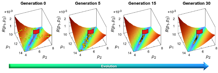
The applied algorithm finds succefully the desired individual corresponding to the Lennard-Jones potential. As seen from the scheme given in Fig. 4, the global minimum of the landscape $R(p_{1},p_{2})$ corresponding to the Lennard-Jones potential is achieved in the process of evolution with fifteen generations. Further, in the process of evolution over ninety generations, the accuracy of the found parameters $p_{1}=12.0$ and $p_{2}=6.0$ is $\pm 10^{-5}$. All the individuals of the “final generation” are within a clear recognizable narrow range containing the desired individual $u_{\text{LJ}}(r)$. This is evidence of the efficiency of the proposed algorithm and indicates the successful solution of the problem formulated above in Sec. 3.1.

The results obtained lead to the question: Is there a one-to-one correspondence between the potential of interaction and the physical properties of the system? The answer to this question seems to be important even in the case of a simple monatomic system, where the interaction of an arbitrary pair of particles is determined only by their mutual distance, as in the case of the Lennard-Jones system. Let us try to get an answer to this question using the Lennard-Jones system as an example.

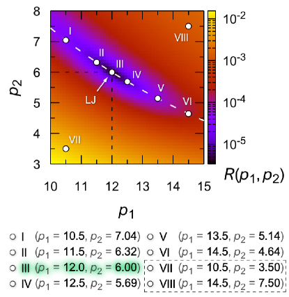
We start with the found residual $R(p_{1},p_{2})$, which quantitatively characterizes the degree of correspondence between the structure of the Mie system and the structure of the Lennard-Jones fluid. The best correspondence will be for such values of the parameters $p_{1}$ and $p_{2}$ for which the landscape $R(p_{1},p_{2})$ has a minimum. As seen in Fig. 5, there is a depression (minimum) on the smooth landscape $R(p_{1},p_{2})$, which is not localized, but is represented by a narrow valley. It is quite natural that in this valley there is the point III corresponding to the Lennard-Jones system. The orientation of the valley in the phase space $(p_{1},p_{2})$ is such that, when moving along it, an increase in the parameter $p_{1}$ is compensated by a decrease in the parameter $p_{2}$, and vice versa. As it turns out, such a correspondence between the parameters $p_{1}$ and $p_{2}$ results in a relatively conserved character of interparticle interaction, which is of the Lennard-Jones type. Let us choose six points (I – VI) along the valley and two points (VII and VIII) maximally remote from the valley as shown in Fig. 5 and consider further the structural, dynamic, and transport properties of the systems, which are determined by the values of the parameters of the Mie potential corresponding to these $(p_{1},p_{2})$ points.

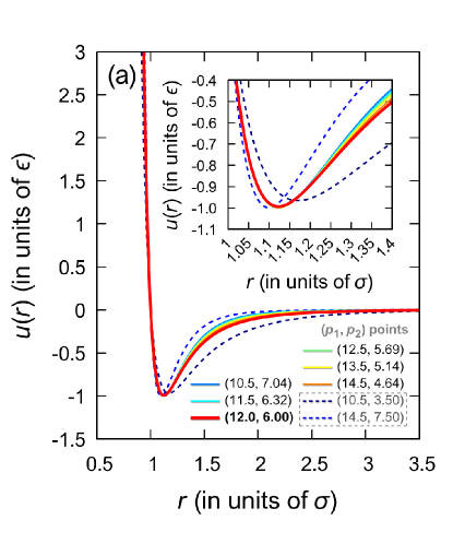
In Fig. 6(a), the Mie potential is shown for the eight combinations of the parameters $p_{1}$ and $p_{2}$ defined in Fig. 5. For points $(p_{1},p_{2})$, marked with symbols I-VI, the general form of the Mie potential is practically the same, and only at the distances $r\sim 1.6\,\sigma$, correlated with the outer boundary of the first coordination sphere, very slight differences are found. Further, the minimum in the Mie potential will be located as in the Lennard-Jones potential at the distance $r_{0}=\sqrt[6]{2}\,\sigma$, if the following equality is satisfied:

$$\left(\frac{p_{1}}{p_{2}}\right)^{1/(p_{1}-p_{2})}=2^{1/6}.$$

(12)

Solving this equation, we find the correspondence between the parameters of the Mie potential:

$$p_{2}=-\frac{6}{\ln{2}}\;W\left(-\frac{\ln{2}}{6}\frac{p_{1}}{2^{\,p_{1}/6}}\right),$$

(13)

where $W(\ldots)$ is the Lambert $W$ function [60]. As can be seen from Fig. 5, Eq. (13) accurately reproduces the location of the valley bottom, where the function $R(p_{1},p_{2})$ takes the minimum values and the best match between the Mie and Lennard-Jones potentials is found. Thus, at least for the range defined by $p_{1}\in[10.5,14.5]$ and $p_{2}\in[4.6,7.0]$, the Mie potential with parameters $p_{1}$ and $p_{2}$ satisfying Eq. (13) reproduces the interparticle interactions almost identical to the Lennard-Jones ones.

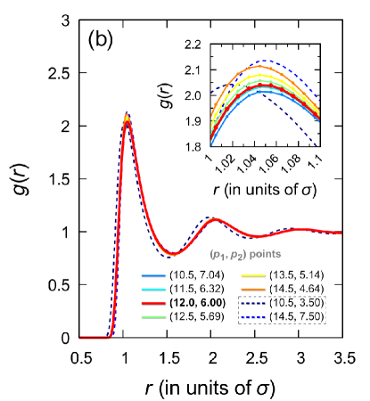
All structural features of the systems along the line containing points I-VI are practically identical. This is well confirmed by the radial distribution functions presented in Fig. 6(b). It is noteworthy that even when the repulsive and attractive contributions of the Mie potential $u(r)$ mutually exceed the Lennard-Jones ones within certain limits, this can nevertheless lead to a radial distribution function $g(r)$ typical of a Lennard-Jones fluid. This is seen, for example, for the case of point VIII with $p_{1}=14.5$ and $p_{2}=7.5$ shown in Fig. 6(b).

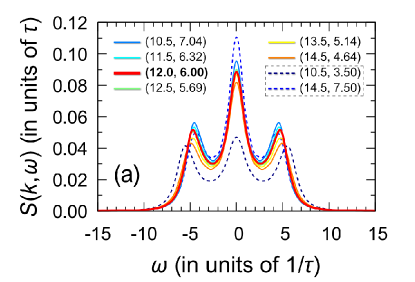
As known, the transport properties and collective dynamics of particles are extremely sensitive to all the nuances of interparticle interactions [61, 62, 63, 64, 65, 66, 67, 68]. The six Mie potentials corresponding to six points I-VI produce typical Lennard-Jones-like collective particle dynamics. This is confirmed by the spectra of the dynamic structure factor $S(k,\omega)$ calculated by means of molecular dynamics simulations with the different Mie potentials. The widths of all peaks and the positions of high-frequency peaks in the spectra of the dynamic structure factor, shown in Fig. 7(a) for the case of the wavenumber $k=(0.68\pm 0.02)\;\sigma^{-1}$ as an example, are practically the same. Insignificant differences are observed only in the intensities of the central (Rayleigh) and high-frequency (Brillouin) components. The coincidence of the spectra of the dynamical structure factor indicates that the collective dynamics of these systems will be also identical to the Lennard-Jones one. The results of Fig. 7a directly indicate that all of these six Mie potentials should reproduce the sound propagation velocity, sound attenuation, and thermal conductivity typical of a Lennard-Jones fluid. The sound velocities for these Mie systems, estimated from molecular dynamics simulations, are as follows¹¹1The sound velocity $v_{s}$ was evaluated from the dispersion law $\omega_{c}=\lim_{k\to 0}v_{s}k$, where $\omega_{c}$ is the location of the Brillouin peak of the dynamic structure factor $S(k,\omega)$ at the generalized hydrodynamics low-$k$ regime.:

	$\displaystyle v_{s}=$	$\displaystyle(6.93\pm 0.33)\,\sqrt{\epsilon/m}$	$\displaystyle\text{for the points I-VI},$
	$\displaystyle v_{s}=$	$\displaystyle(8.11\pm 0.2)\,\sqrt{\epsilon/m}$	$\displaystyle\text{for the point VII},$

and

$$v_{s}=(6.42\pm 0.2)\,\sqrt{\epsilon/m}\quad\text{for the point VIII}.$$

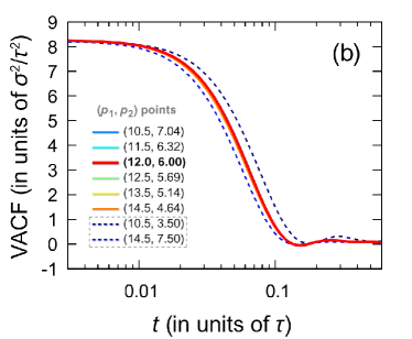
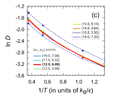
For the points I-VI, the same sound velocities, as well as the similar shapes of the high-frequency peak of the dynamic structure factor, indicate the same character of the propagation and attenuation of acoustic-like waves in the systems corresponding to the points I-VI. It is noteworthy that the velocity autocorrelation function, which characterizes the single-particle dynamics, also turns out to be the same for the potentials I-VI [see Fig. 7(b)]. Considering these results on the structure and particle dynamics, it can be expected that the Mie potentials (I-VI) are able even for a range of temperatures to reproduce the physical properties typical of the Lennard-Jones system. Indeed, as can be seen in Fig. 7(c), the self-diffusion coefficient $D$ calculated on the basis of the molecular dynamics simulations data along the isochore ($\rho^{-1}=1.18\,\sigma^{3}$ per particle) over a wide temperature range turns out to be the same for these systems. Thus, the Mie potentials I-VI lead to the single-particle dynamics and mass transport properties identical to those for the Lennard-Jones fluid.

References

- [1] L. D. Landau, E. M. Lifshitz, Course of Theoretical Physics: Vol. 5, Statistical Physics, Part 1, Butterworth-Heinemann, Oxford, 1980.
- [2] D. J. Evans, G. P. Morris, Statistical Mechanics of Nonequilibrium Liquids, Academic Press, London, 1990.
- [3] K. Binder, W. Kob, Glassy Materials and Disordered Solids: An Introduction to Their Statistical Mechanics, World Scientific, Singapore, 2011.
- [4] J. G. Kirkwood, The Statistical Mechanical Theory of Transport Processes I. General Theory, J. Chem. Phys. 14 (1946) 180–201. https://doi.org/10.1063/1.1724117
- [5] J.-P. Hansen, I. R. McDonald, Theory of Simple Liquids, Academic Press, London, 2006.
- [6] I. I. Fairushin, S. A. Khrapak, A. V. Mokshin, Direct evaluation of the physical characteristics of Yukawa fluids based on a simple approximation for the radial distribution function, Results in Physics 19 (2020) 103359. https://doi.org/10.1016/j.rinp.2020.103359
- [7] A. V. Mokshin, I. I. Fairushin, I. M. Tkachenko, Self-consistent relaxation theory of collective ion dynamics in Yukawa one-component plasmas under intermediate screening regimes, Phys. Rev. E 105 (2022) 025204. https://doi.org/10.1103/PhysRevE.105.025204
- [8] C. N. Likos, Effective interactions in soft condensed matter physics, Phys. Rep. 348 (2001) 207. https://doi.org/10.1016/S0370-1573(00)00141-1
- [9] T. Mueller, A. Hernandez, C. Wang, Machine learning for interatomic potential models, J. Chem. Phys. 152 (2020) 050902. https://doi.org/10.1063/1.5126336
- [10] J. Behler, Perspective: Machine learning potentials for atomistic simulations, J. Chem. Phys. 145 (2016) 170901. https://doi.org/10.1063/1.4966192
- [11] P. Rowe, G. Csányi, D. Alfè, A. Michaelides, Development of a machine learning potential for graphene, Phys. Rev. B 97 (2018) 054303. https://doi.org/10.1103/PhysRevB.97.054303
- [12] V. L. Deringer, A. P. Bartòk, N. Bernstein, D. M. Wilkins, M. Ceriotti, G. Csányi, Gaussian Process Regression for Materials and Molecules, Chem. Rev. 121 (2021) 10073–10141. https://doi.org/10.1021/acs.chemrev.1c00022
- [13] F. Ercolessi, J. B. Adams, Interatomic Potentials from First-Principles Calculations: The Force-Matching Method, Europhys. Lett. 26 (1994) 583–588. https://doi.org/10.1209/0295-5075/26/8/005
- [14] T. B. Blank, S. D. Brown, A. W. Calhoun, D. J. Doren, Neural network models of potential energy surfaces, J. Chem. Phys. 103 (1995) 4129–4137. https://doi.org/10.1063/1.469597
- [15] R. E. Ryltsev, N. M. Chtchelkatchev, Deep machine learning potentials for multicomponent metallic melts: Development, predictability and compositional transferabilit, J. Mol. Liq. 349 (2022) 118181. https://doi.org/10.1016/j.molliq.2021.118181
- [16] C. Groetsch, Inverse Problems: Activities for Undergraduates, The Mathematical Association of America, 1999.
- [17] R. L. McGreevy, L. Pusztai, Reverse Monte Carlo Simulation: A New Technique for the Determination of Disordered Structures, Mol. Simulat. 1 (1988) 359–367. https://doi.org/10.1080/08927028808080958
- [18] A. P. Lyubartsev, A. Laaksonen, Calculation of effective interaction potentials from radial distribution functions: A reverse Monte Carlo approach, Phys. Rev. E 52 (1995) 3730–3737. https://doi.org/10.1103/PhysRevE.52.3730
- [19] T. Youngs, Dissolve: next generation software for the interrogation of total scattering data by empirical potential generation, Molecular Physics 117 (2019) 3464–3477. https://doi.org/10.1080/00268976.2019.1651918
- [20] D. Levesque, J. J. Weis, L. Reatto, Pair interaction from structural data for dense classical liquids, Phys. Rev. Lett. 54 (1985) 451–454. https://doi.org/10.1103/physrevlett.54.451
- [21] M.-C. Chang, C. H. Tung, S. Y. Chang, J. M. Carrillo, Y. Wang, B. G. Sumpter, G.-R. Huang, C. Do, W.-R. Chen, A machine learning inversion scheme for determining interaction from scattering, Commun. Phys. 5 (2022) 46. https://doi.org/10.1038/s42005-021-00778-y
- [22] A. K. Soper, Empirical potential Monte Carlo simulation of fluid structure, Chem. Phys. 202 (1996) 295–306. https://doi.org/10.1016/0301-0104(95)00357-6
- [23] H. Chan, M. J. Cherukara, B. Narayanan, T. D. Loeffler, C. Benmore, S. K. Gray, S. K. R. S. Sankaranarayanan, Machine learning coarse grained models for water, Nat. Commun. 10 (2019) 379. https://doi.org/10.1038/s41467-018-08222-6
- [24] S. Thaler, J. Zavadlav, Learning neural network potentials from experimental data via Differentiable Trajectory Reweighting, Nat. Commun. 12 (2021) 6884. https://doi.org/10.1038/s41467-021-27241-4
- [25] D. R. de Assis Elias, E. Granato, M. de Koning, Global exploration of phase behavior in frustrated Ising models using unsupervised learning techniques, Physica A 589 (2022) 126653. https://doi.org/10.1016/j.physa.2021.126653
- [26] Y. Jiang and M. T. Sulgani, R. Ranjbarzadeh, A. Karimipour, T. K. Nguyen, Hybrid GMDH-type neural network to predict fluid surface tension, shear stress, dynamic viscosity & sensitivity analysis based on empirical data of iron(II) oxide nanoparticles in light crude oil mixture, Physica A 526 (2019) 120948. https://doi.org/10.1016/j.physa.2019.04.184
- [27] C. O. Stoico, D. G. Renzi, F. Vericat, A genetic algorithm for the 1D electron gas, Physica A 387 (2008) 159–166. https://doi.org/10.1016/j.physa.2007.07.075
- [28] I. Grigorenko, M. E. Garcia, An evolutionary algorithm to calculate the ground state of a quantum system, Physica A 284 (2000) 131–139. https://doi.org/10.1016/S0378-4371(00)00218-1
- [29] W. Yu, P. Lyu, Unsupervised machine learning of phase transition in percolation, Physica A 559 (2020) 125065. https://doi.org/10.1016/j.physa.2020.125065
- [30] D. Yadav, P. Dansena, S. K. Ghosh, P. K. Singh, A unique multilayer perceptron model (ANN) for different oxide/EG nanofluid’s viscosity from the experimental study, Physica A 549 (2020) 124030. https://doi.org/10.1016/j.physa.2019.124030
- [31] F. Sofos, A. Charakopoulos, K. Papastamatiou, T. E. Karakasidis, A combined clustering/symbolic regression framework for fluid property prediction, Phys. Fluids 34 (2022) 062004. https://doi.org/10.1063/5.0096669
- [32] T. M. Alam, J. P. Allers, C. J. Leverant, J. A. Harvey, Symbolic regression development of empirical equations for diffusion in Lennard-Jones fluids, J. Chem. Phys. 157 (2022) 014503. https://doi.org/10.1063/5.0093658
- [33] K. Papastamatiou, F. Sofos, T. E. Karakasidis, Machine learning symbolic equations for diffusion with physics-based descriptions, AIP Adv. 12 (2022) 025004. https://doi.org/10.1063/5.0082147
- [34] R. Storn, K. Price, Differential Evolution — A Simple and Efficient Heuristic for global Optimization over Continuous Spaces, J. Global Optim. 11 (1997) 341–359. https://doi.org/10.1023/A:1008202821328
- [35] I. A. Kruglov, A. Yanilkin, A. R. Oganov, P. Korotaev, Phase diagram of uranium from ab initio calculations and machine learning, Phys. Rev. B 100 (2019) 174104. https://doi.org/10.1103/PhysRevB.100.174104
- [36] H. Wang, X.-L. Pan, Y.-F. Wang, X.-R. Chen, Y.-X. Wang, H.-Y. Geng, Lattice dynamics and elastic properties of -U at high-temperature and high-pressure by machine learning potential simulations, J. Nucl. Mater. 572 (2022) 154029. https://doi.org/10.1016/j.jnucmat.2022.154029
- [37] N. Van Nghia, H. K. Hieu, The melting curves of tin, uranium, cadmium, thallium and indium metals under pressure, Chem. Phys. 553 (2022) 111389. https://doi.org/10.1016/j.chemphys.2021.111389
- [38] B. Beeler, K. Mahbuba, Y. Wang, A. Jokisaari, Determination of Thermal Expansion, Defect Formation Energy, and Defect-Induced Strain of -U Via ab Initio Molecular Dynamics, Front. Mater. 8 (2021) 661387. https://doi.org/10.3389/fmats.2021.661387
- [39] K. Migdal, A. Yanilkin, Cold and hot uranium in DFT calculations: Investigation by the GTH pseudopotential, PAW, and APW + lo methods, Comput. Mater. Sci. 199 (2021) 110665. https://doi.org/10.1016/j.commatsci.2021.110665
- [40] A. J. Clark, J. McCarty, M. G. Guenza, Effective potentials for representing polymers in melts as chains of interacting soft particles, J. Chem. Phys. 139 (2013) 124906. https://doi.org/10.1063/1.4821818
- [41] J. Jin, A. J. Pak, A. E. P. Durumeric, T. D. Loose, G. A. Voth, Bottom-up Coarse-Graining: Principles and Perspectives, J. Chem. Theory Comput. XXX (2022) XXX. https://doi.org/10.1021/acs.jctc.2c00643
- [42] S. Y. Joshi, S. A. Deshmukh, A review of advancements in coarse-grained molecular dynamics simulations, 47 (2021) 786-803. https://doi.org/10.1080/08927022.2020.1828583
- [43] I. Z. Fisher, Statistical Theory of Liquids, University of Chicago Press, Chicago, IL, 1964.
- [44] J. P. Boon, S. Yip, Molecular Hydrodynamics, Dover Publications, New York, 1991.
- [45] J. A. Barker, D. Henderson, What is “liquid”? Understanding the states of matter, Rev. Mod. Phys. 48 (1976) 587–671. https://doi.org/10.1103/RevModPhys.48.587
- [46] M. P. Allen, D. J. Tildesley, Computer Simulation of Liquids, Oxford University Press, Oxford, 1991.
- [47] D. Frenkel and B. Smit, Understanding Molecular Simulation: From Algorithms to Applications, Academic Press, San Diego, 2002.
- [48] N. R. Draper and H. Smith, Applied Regression Analysis, John Wiley & Sons, 1998.
- [49] S. Plimpton, Fast Parallel Algorithms for Short-Range Molecular Dynamics, J. Comp. Phys. 117 (1995) 1–19. https://doi.org/10.1006/jcph.1995.1039
- [50] T. Bäck, Evolutionary Algorithms in Theory and Practice: Evolution Strategies, Evolutionary Programming, Genetic Algorithms, Oxford University Press, Oxfrod, 1996.
- [51] K. V. Price, R. M. Storn and J. A. Lampinen, Differential Evolution: A Practical Approach to Global Optimization, Springer, Berlin, 2005.
- [52] K. V. Price, Differential evolution: a fast and simple numerical optimizer, NAFIPS’96 (1996) 524–527. https://doi.org/10.1109/NAFIPS.1996.534790
- [53] D. H. Ackley, A connectionist machine for genetic hillclimbing, Kluwer Academic Publishers, Boston, 1987.
- [54] M. Centeno-Telleria, E. Zulueta, U. Fernandez-Gamiz, D. Teso-Fz-Betono, A. Teso-Fz-Betono, Differential Evolution Optimal Parameters Tuning with Artificial Neural Network, Mathematics 9 (2021) 427. https://doi.org/10.3390/math9040427
- [55] G. Mie, Zur kinetischen Theorie der einatomigen Körper, Ann. Phys. 11 (1903) 657–697. https://doi.org/10.1002/andp.19033160802
- [56] K. Trachenko, V. V. Brazhkin, Collective modes and thermodynamics of the liquid state, Rep. Prog. Phys. 79 (2016) 016502. https://doi.org/10.1088/0034-4885/79/1/016502
- [57] S. Stephan, M. Thol, J. Vrabec, H. Hasse, Thermophysical Properties of the Lennard-Jones Fluid: Database and Data Assessment, J. Chem. Inf. Model. 59 (2019) 4248–4265. https://doi.org/10.1021/acs.jcim.9b00620
- [58] A. J. Schultz, D. A. Kofke, Comprehensive high-precision high-accuracy equation of state and coexistence properties for classical Lennard-Jones crystals and low-temperature fluid phases, J. Chem. Phys. 149 (2018) 204508. https://doi.org/10.1063/1.5053714
- [59] S. Toxvaerd, J. C. Dyre, Communication: Shifted forces in molecular dynamics, J. Chem. Phys. 134 (2011) 081102. https://doi.org/10.1063/1.3558787
- [60] D. Veberič, Lambert W function for applications in physics, Comput. Phys. Commun. 183 (2012) 2622–2628. https://doi.org/10.1016/j.cpc.2012.07.008
- [61] P. Gallo, R. Pellarin, M. Rovere, Single particle dynamics of a confined Lennard–Jones mixture in the supercooled regime, Physica A 314 (2002) 530–538. https://doi.org/10.1016/S0378-4371(02)01046-4
- [62] Y. D. Fomin, V. V. Ryzhov, E. N. Tsiok, V. V. Brazhkin, Dynamical crossover line in supercritical water, Sci. Rep. 5 (2015) 14234. https://doi.org/10.1038/srep14234
- [63] A. V. Mokshin, Self-consistent approach to the description of relaxation processes in classical multiparticle systems, Theor. Math. Phys. 183 (2015) 449–477. https://doi.org/10.4213/tmf8778
- [64] A. V. Mokshin, B. N. Galimzyanov, A method for analyzing the non-stationary nucleation and overall transition kinetics: A case of water, J. Chem. Phys. 140 (2014) 024104. https://doi.org/10.1063/1.4851438
- [65] A. V. Mokshin, B. N. Galimzyanov, Self-consistent description of local density dynamics in simple liquids. The case of molten lithium, J. Phys.: Condens. Matter 30 (2018) 085102. https://doi.org/10.1088/1361-648X/aaa7bc
- [66] R. M. Khusnutdinoff, B. N. Galimzyanov, A. V. Mokshin, Dynamics of Liquid Lithium Atoms. Pseudopotential and EAM-Type Potentials, J. Exp. Theor. Phys. 126 (2018) 83–89. https://doi.org/10.1134/S1063776118010041
- [67] R. M. Khusnutdinoff, A. V. Mokshin, B. A. Klumov, R. E. Ryltsev, N. M. Chtchelkatchev, Structural features and the microscopic dynamics of the three-component Zr47Cu46Al7 system: Equilibrium melt, supercooled melt, and amorphous alloy, J. Exp. Theor. Phys. 123 (2016) 265–276. https://doi.org/10.1134/S1063776116060042
- [68] A. V. Mokshin, S. O. Zabegaev, R. M. Khusnutdinoff, Dynamic heterogeneity of a colloidal solution near the sol-gel transition, Phys. Solid State 53 (2011) 570–576. https://doi.org/10.1134/S106378341103019X