Isolated Skyrmions in the nonlinear -model with a Dzyaloshinskii-Moriya type interaction
Abstract
We study two dimensional soliton solutions in the nonlinear -model with a Dzyaloshinskii-Moriya type interaction. First, we derive such a model as a continuous limit of the tilted ferromagnetic Heisenberg model on a square lattice. Then, introducing an additional potential term to the derived Hamiltonian, we obtain exact soliton solutions for particular sets of parameters of the model. The vacuum of the exact solution can be interpreted as a spin nematic state. For a wider range of coupling constants, we construct numerical solutions, which possess the same type of asymptotic decay as the exact analytical solution, both decaying into a spin nematic state.
1 Introduction
In the 1960s, Skyrme introduced a (3+1)-dimensional nonlinear (NL) -model [1, 2] which is now well-known as a prototype of a classical field theory that supports topological solitons (See Ref. [3], for example). Historically, the Skyrme model has been proposed as a low-energy effective theory of atomic nuclei. In this framework, the topological charge of the field configuration is identified with the baryon number.
The Skyrme model, apart from being considered a good candidate for the low-energy QCD effective theory, has attracted much attention in various applications, ranging from string theory and cosmology to condensed matter physics. One of the most interesting developments here is related to a planar reduction of the NL-model, the so-called baby Skyrme model [4, 5, 6]. This (2+1)-dimensional simplified theory resembles the basic properties of the original Skyrme model in many aspects.
The baby Skyrme model finds a number of physical realizations in different branches of modern physics. Originally, it was proposed as a modification of the Heisenberg model [7, 4, 5]. Then, it was pointed out that Skyrmion configurations naturally arise in condensed matter systems with intrinsic and induced chirality [8, 9, 10, 11, 12]. These baby Skyrmions, often referred to as magnetic Skyrmions, were experimentally observed in non-centrosymmetric or chiral magnets [13, 14, 15]. This discovery triggered extensive research on Skyrmions in magnetic materials. This direction is a rapidly growing area both theoretically and experimentally [16].
A typical stabilizing mechanism of magnetic skyrmions is the existence of Dzyaloshinskii-Moriya (DM) interaction [17, 18], which stems from the spin-orbit coupling. In fact, the magnetic Skyrmions in chiral magnets can be well described by the continuum effective Hamiltonian
| (1.1) |
where is a three component unit magnetization vector which corresponds to the spin expectation value at position . The first term in Eq. (1.1) is the continuum limit of the Heisenberg exchange interaction, i.e., the kinetic term of the NL-model, which is often referred to as the Dirichlet term. The second term there is the DM interaction term, the third one is the Zeeman coupling with an external magnetic field , and the last, symmetry breaking term represents the uniaxial anisotropy.
It is remarkable that in the limiting case , the Hamiltonian (1.1) can be written as the static version of the gauged NL-model [19, 20]
| (1.2) |
with a background gauge field . Though the DM term is usually introduced phenomenologically, a mathematical derivation of the Hamiltonian (1.2) with arbitrary has been developed recently [19], i.e.; it has been shown that the Hamiltonian can be derived mathematically in a continuum limit of the tilted (quantum) Heisenberg model
| (1.3) |
where the sum is taken over the nearest-neighbor sites, denotes the -th component of spin operators at site and . It was reported that the tilting Heisenberg model can be derived from a Hubbard model at half-filling in the presence of spin-orbit coupling [21]. Therefore, the background field can still be interpreted as an effect of the spin-orbit coupling.
There are two advantages of utilizing the expression (1.2) for the theoretical study of baby Skyrmions in the presence of the so-called Lifshitz invariant, an interaction term which is linear in a derivative of an order parameter [22, 23], like the DM term. The first advantage of the form Eq. (1.2) is that one can study a NL-model with various form of Lifshitz invariants which are mathematically derived by choice of the background field , although Lifshitz invariants have, in general, a phenomenological origin corresponding to the crystallographic handedness of a given sample. The second advantage of the model (1.2) is that it allows us to employ several analytical techniques developed for the gauged NL-model. It has been recently reported in Ref. [20] that the Hamiltonian (1.2) with a specific choice of the potential term exactly satisfies the Bogomol’nyi bound, and the corresponding Bogomol’nyi-Prasad-Sommerfield (BPS) equations have exact closed-form solutions [20, 24, 25].
Geometrically, the planar Skyrmions are very nicely described in terms of the complex field on the compactified domain space [6]. Further, there are various generalizations of this model; for example, two-dimensional Skyrmions have been studied in the pure NL-model [26, 27, 28] and in the Faddeev-Skyrme type model [29, 30].
Remarkably, the two dimensional NL-model can be obtained as a continuum limit of the ferromagnetic (FM) Heisenberg model [31, 32] on a square lattice defined by the Hamiltonian
| (1.4) |
where is a positive constant, and () stand for the spin operators of the fundamental representation at site satisfying the commutation relation
| (1.5) |
Here, the structure constants are given by , where are the usual Gell-Mann matrices.
The FM Heisenberg model may play an important role in diverse physical systems ranging from string theory [33] to condensed matter, or quantum optical three-level systems [34]. It can be derived from a spin-1 bilinear-biquadratic model with a specific choice of coupling constants, so-called FM point, see, e.g., Ref. [35]. The spin operators can be defined in terms of the spin operators () as
| (1.6) |
Using the commutation relation where denotes the anti-symmetric tensor, one can check that the operators (1.6) satisfy the commutation relation (1.5).
In the present paper, we study baby Skyrmion solutions of an extended NL-model composed of the Dirichlet term, a DM type interaction term, i.e., the Lifshitz invariant, and a potential term. The Lifshitz invariant, instead of being introduced ad hoc in the continuum Hamiltonian, can be derived in a mathematically well-defined way via consideration of a continuum limit of the tilted Heisenberg model. Below we will implement this approach in our derivation of the Lifshitz invariant. In the extended NL-model, we derive exact soliton solutions for specific combinations of coupling constants called the BPS point and solvable line. For a broader range of coupling constants, we construct solitons by solving the Euler-Lagrange equation numerically.
The organization of this paper is the following: In the next section, we derive an gauged NL-model from the tilted Heisenberg model. Similar to the case described as Eq. (1.2), the term linear in a background field can be viewed as a Lifshitz invariant term. In Sec. 3, we study exact Skyrmionic solutions of the gauged NL-model in the presence of a potential term for the BPS point and solvable line using the BPS arguments. The numerical construction of baby Skyrmion solutions off the solvable line is given in Sec. 4. Our conclusions are given in Sec. 5.
2 Gauged NL-model from a spin system
To find Lifshitz invariant terms relevant for the NL-model, we begin to derive an gauged NL-model, a generalization of Eq. (1.2), from a spin system on a square lattice. By analogy with Eq. (1.2), the Lifshitz invariant, in that case, can be introduced as a term linear in a non-dynamical background gauge potential of the gauged model.
Following the procedure to obtain a gauged NL-model from a spin system, as discussed in Ref. [19], we consider a generalization of the Heisenberg model defined by the Hamiltonian
| (2.1) |
where is a background field which can be recognized as a Wilson line operator along with the link from the point to the point , which is an element of the group in the adjoint representation. As in the case [19], the field may describe effects originated from spin (nematic)-orbital coupling, complicated crystalline structure, and so on. This Hamiltonian can be viewed as the exchange interaction term for the tilted operator where , because one can write where is an element of in the adjoint representation. Clearly, , where stands for the transposition.
Let us now find the classical counterpart of the quantum Hamiltonian (2.1). It can be defined as an expectation value of Eq. (2.1) in a state possessing over-completeness, through a path integral representation of the partition function. In order to construct such a state for the spin-1 system, it is convenient to introduce the Cartesian basis
| (2.2) |
where (, ). In terms of the Cartesian basis, an arbitrary spin-1 state at a site can be expressed as a linear combination where stands for the position of the site , and is a complex vector of unit length [36, 31]. Since the state satisfies an over-completeness relation, one can obtain the classical Hamiltonian using the state
| (2.3) |
Since is normalized and has the gauge degrees of freedom corresponding to the overall phase factor multiplication, it takes values in . In terms of the basis (2.2), the spin operators can be defined as
| (2.4) |
where is the -th component of the Gell-Mann matrices. One can check that they satisfy the commutation relation (1.5). The expectation values of the operators in the state (2.3) are given by
| (2.5) |
where denotes the complex conjugation of . In the context of QCD, the field is usually termed a color (direction) field [37]. The color field satisfies the constraints
| (2.6) |
where . Consequently, the number of degrees of freedom of the color field reduces to four. Note that, combining the constraints (2.6), one can get the Casimir identity .
In terms of the color field, the classical Hamiltonian is given by
| (2.7) |
Let us write the position of a site next to a site as where is the unit vector in the -th direction, , and stands for the lattice constant. For , the field can be approximated by the exponential expansion
| (2.8) |
where is the unit matrix and are the generators of in the adjoint representation, i.e., . In addition, since the model (2.1) is ferromagnetic, it is natural to assume that nearest-neighbor spins are oriented in the almost same direction, which allows us to use the Taylor expansion
| (2.9) |
Replacing the sum over the lattice sites in Eq. (2.7) by the integral , we obtain a continuum Hamiltonian, except for a constant term, of the form
| (2.10) |
where and . Similar to its counterpart expressed as Eq. (1.2), this Hamiltonian can also be written as the static energy of an gauged NL-model
| (2.11) |
where is the covariant derivative. Since the Hamiltonian is given by the covariant derivative, Eq. (2.11) is invariant under the gauge transformation
| (2.12) |
where . Note that, however, since the Hamiltonian (2.11) does not include kinetic terms for the gauge field, like the Yang-Mills term, or the Chern-Simons term, the gauge potential is just a background field, not the dynamical one. We suppose that the gauge field is fixed beforehand by the structure of a sample and give the value by hand, like the case. The gauge fixing allows us to recognize the second term in Eq. (2.10) as a Lifshitz invariant term.
We would like to emphasize that we do not deal with Eq. (2.11) as a gauge theory. Rather, we deem it the NL-model with a Lifshitz invariant, and show the existence of the exact and the numerical solutions. For the baby Skyrmion solutions we shall obtain, the color field approaches to a constant value at spatial infinity so that the physical space can be topologically compactified to . Therefore, they are characterized by the topological degree of the map given by
| (2.13) |
Combining with the assumption that the gauge is fixed, it is reasonable to identify this quantity (2.13) with the topological charge in our model111 If one extends the model (2.11) with a dynamical gauge field, the topological charge is defined by the gauge invariant quantity which is directly obtained by replacing the partial difference in Eq. (2.13) with the covariant derivative..
3 Exact solutions of the gauged NL-model
In this section, we derive exact solutions of the model with the Hamiltonian (2.11) supplemented by a potential term. We first remark on the validity of the variational problem. As discussed in Refs. [20, 25] for the case, a surface term, which appears in the process of variation, cannot be ignored if the physical space is non-compact and the gauge potential does not vanish at the spatial infinity like the DM term. This problem can be cured by introducing an appropriate boundary term, like [20]
| (3.1) |
where . Here the gauge potential satisfies
| (3.2) |
where is the asymptotic value of at spatial infinity. Note that Eq. (3.2) corresponds to the asymptotic form of the BPS equation, which we shall discuss in the next subsection. Hence, all field configurations we consider in this paper satisfy this equation automatically.
Since (3.1) is a surface term, it does not contribute to the Euler-Lagrange equation, i.e., the classical Heisenberg equation. Note that the solutions derived in the following sections satisfy Derrick’s scaling relation with the boundary term, which is obtained by keeping the background field intact under the scaling, i. e., where denotes the energy contribution from the first derivative terms including the boundary term (3.1) and from no derivative terms.
3.1 BPS solutions
Recently, it has been proved that the gauged NL-model (1.2) possesses BPS solutions in the presence of a particular potential term [20, 24]. Here, we show that BPS solutions also exist in the gauged model with a special choice of the potential term, which is given by
| (3.3) |
where . As we shall see in the next subsection, the potential term can possess a natural physical interpretation for some background gauge field. It follows that the Hamiltonian we study here reads
| (3.4) |
where the double-sign corresponds to that of Eq. (3.1).
First, let us show that the lower energy bound of Eq. (3.4) is given by the topological charge (2.13). The first term in Eq. (3.4) can be written as
| (3.5) |
It follows that the equality is satisfied if
| (3.6) |
which reduces to Eq. (3.2) at the spatial infinity. Therefore, one obtains the lower bound of the form
| (3.7) |
where the corresponding BPS equation is given by Eq. (3.6). Note that, unlike the energy bound of the self-dual solutions [7, 27], the energy bound (3.7) can be negative, and it is not proportional to the absolute value of the topological charge.
As is often the case in two-dimensional BPS equations [7, 20], solutions can be best described in terms of the complex coordinates . Further, we make use of the associated differential operator and background field defined as and . Then, the BPS equation (3.6) can be written as
| (3.8) |
Similar to the case [20], Eq. (3.8) with a plus sign can be solved if the background field has the form
| (3.9) |
where . Note that Eq. (3.9) is not necessarily a pure gauge. Similarly, Eq. (3.8) with the minus sign on the right-hand side can be solved if . For the background field (3.9), one finds that the BPS equation (3.8) is equivalent to
| (3.10) |
because, under the gauge transformation, the fields are changed as and . In the following, we only consider Eq. (3.9) to simplify our discussion.
In order to solve the equation (3.10), we introduce a tractable parameterization of the color field
| (3.11) |
with , where is the continuum counter part of the vector in Eq. (2.3) and are vectors forming an orthonormal basis for with . Up to the gauge degrees of freedom, the components can be written as
| (3.12) |
Therefore, the vector fully defines the color field . Accordingly, we can write
| (3.13) |
with . It follows that the field , which is the fundamental field of the model, is given by . Substituting the field (3.13) into the equation (3.10), one finds that Eq. (3.10) reduces to the coupled equation
| (3.14) |
where . Since the three vectors form an orthonormal basis, Eq. (3.14) implies where the function is given by Therefore, the equation (3.10) is solved by any configuration satisfying
| (3.15) |
where for arbitrary non-zero vector . Moreover, we write
| (3.16) |
where is a three component unit vector, i.e. . Then, Eq. (3.15) can be reduced to
| (3.17) |
which is the very BPS equation of the standard NL-model. Thus, a general solution of Eq. (3.15), up to the gauge degrees of freedom, is given by
| (3.18) |
where has no overall factor, and is a polynomial in . Therefore, we finally obtain the solution for the field
| (3.19) |
where is a normalization factor.
3.2 Properties of the BPS solutions
As the BPS bound (3.7) indicates, the lowest energy solution among Eq. (3.19) with a given background function possesses the highest topological charge. In terms of the explicit calculation of the topological charge, we discuss the conditions for the lowest energy solutions.
The topological charge (2.13) can be written in terms of as
| (3.20) |
We employ the constant background gauge field for simplicity. Then, the matrix in Eq. (3.9) becomes
| (3.21) |
so that the components of are given by power series in . It allows us to write Eq. (3.20) as a line integral along the circle at spatial infinity
| (3.22) |
with [27, 38], since the one-form becomes globally well-defined. To evaluate the integral in Eq. (3.22), we write explicitly
| (3.23) |
where is the component of the inverse matrix .
Let () be the highest power in (). Note that though are formally represented as power series in , the integers are not always infinite; especially, if a positive integer power of is zero, all of become finite because reduces to a polynomial of finite degree in . Using the plane polar coordinates , one can write at the spatial boundary and find that only the components of the highest power in contribute to the integral (3.22). Since we are interested in constructing topological solitons, we consider the case when the physical space can be compactified to the sphere , i.e., the field takes some fixed value on the spatial boundary. Such a compactification is possible if there is only one pair giving the largest sum or any pairs , sharing the largest sum, have the same value of the difference. For such configurations, the topological charge is given by
| (3.24) |
where the combination yields the largest sum among any pairs . This equation (3.24) indicates that the highest topological charge configuration is given by the choice for a particular value of which gives the biggest .
We are looking for the lowest energy solutions with an explicit background field. As a particular example, let us consider
| (3.25) |
where is a constant. Clearly, this choice yields the potential term
| (3.26) |
which can be interpreted as an easy-axis anisotropy, or quadratic Zeeman term, which naturally appears in condensed matter physics. In this case, the solution (3.19) can be written as
| (3.27) |
Therefore, the solution with the highest topological charge is given by , with , and being a nonzero constant. Choosing , one can obtain the axially-symmetric solution
| (3.28) |
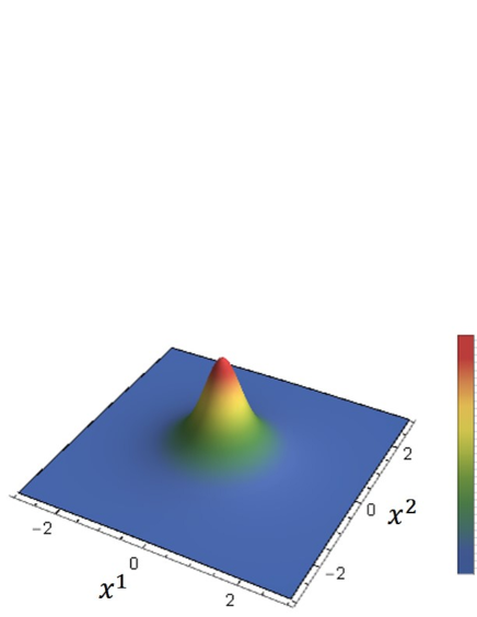
which possesses the topological charge . Note that this configuration also satisfies the BPS equation of the pure NL-model [26, 27, 31]. Figure 1 shows the distribution of the topological charge (3.20) of this solution (3.28) with . We find that the topological charge density has a single peak, although higher charge topological solitons with axial symmetry are likely to possess a volcano structure, see e.g., Ref. [39]. These highest charge solutions give the asymptotic values at spatial infinity of the color field
| (3.29) |
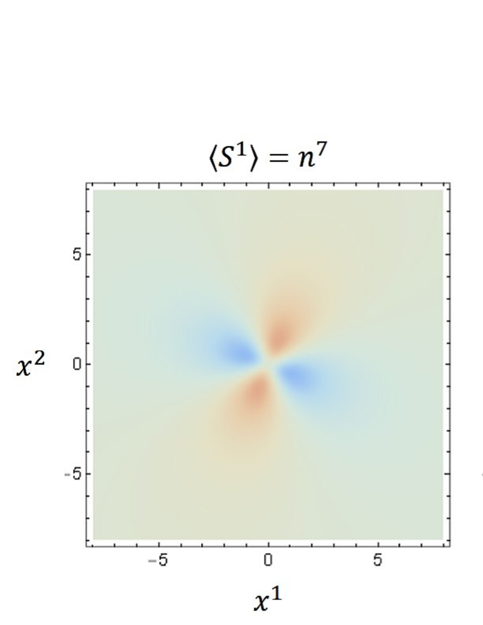
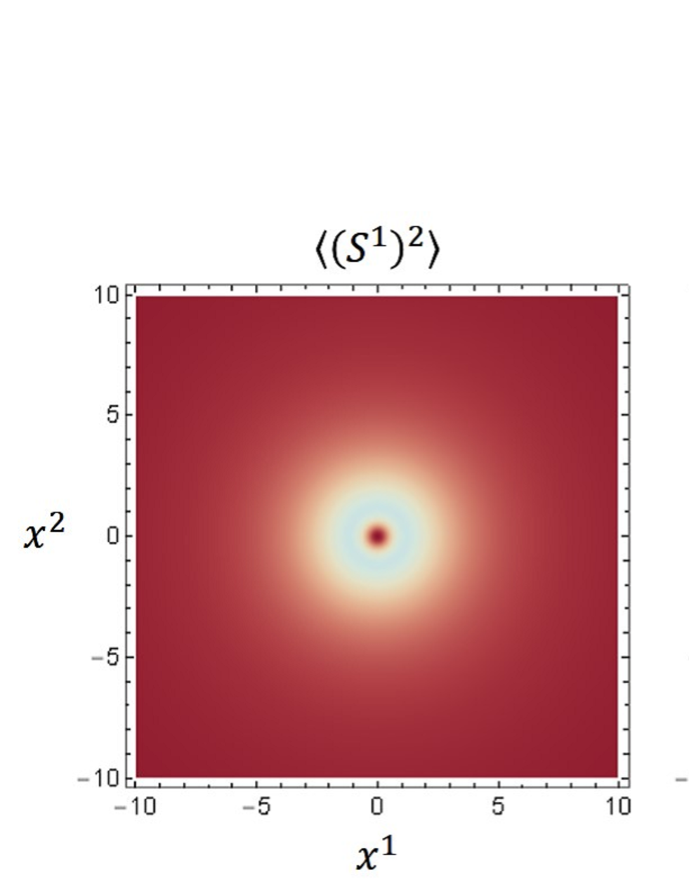
It indicates that takes the vacuum value in the Cartan subalgebra of . Hence, the vacuum of the model corresponds to a spin nematic, i.e., and . Unlike the pure model, there is no degeneracy between the spin nematic state and ferromagnetic state in our model because the global symmetry is broken. As shown in Fig. 2, the spin nematic state is partially broken around the soliton because the expectation values become finite. Fig. 3 shows that of the solution (3.28) are axially symmetric, although the expectation values have angular dependence.
3.3 Exact solutions off the BPS point
Note that the Hamiltonian (1.1) with admits closed-form analytical solutions [40]. Further, the BPS truncation corresponds to the restricted choice of the parameters, . The relation is referred to as the solvable line, whereas the restriction is called the BPS point [25]. Here we show that similar restrictions occur in our model. For this purpose, we consider the generalized Hamiltonian
| (3.30) |
where and are real coupling constants. Here, indicates the Dirichlet term, i.e., the first term in the r.h.s of Eq. (2.10), and does the Lifshitz invariant term which is the second term of that. Explicitly, these and other terms read
| (3.31) | |||
| (3.32) | |||
| (3.33) | |||
| (3.34) |
where is a constant background field, as before. Finally, the boundary term is defined by Eq. (3.1) with the negative sign in the r.h.s., the same as before. Note that we also introduced constant terms in Eqs. (3.33) and (3.34) in order to guarantee the finiteness of the total energy. Clearly, the Hamiltonian (3.30) is reduced to Eq. (3.4) as we set .
The existence of exact solutions of the Hamiltonian (3.30) with can be easily shown if we rescale the space coordinates as , where is a positive constant, while the background gauge field remains intact. By rescaling, the Hamiltonian (3.30) becomes
| (3.35) |
Setting and choosing the scale parameter , one gets
| (3.36) |
Notice that since the solutions (3.19) with being arbitrary constants are holomorphic maps from to , they satisfy not only the variational equations but also the equations , where denotes the variation with respect to with preserving the constraint (2.6). Therefore, the solutions also satisfy the equations . This implies that, in the limit , the Hamiltonian (3.30) supports a family of exact solutions of the form
| (3.37) |
where is a three-component complex unit vector.
Since the solution (3.37) is a BPS solution of the pure model with the positive topological charge , one gets . In addition, the lower bound at the BPS point (3.7) indicates that . Combining these bounds, we find that the total energy of the solution (3.37) is given by
| (3.38) |
Since the energy becomes negative if , we can expect that for small values of the coupling , the homogeneous vacuum state becomes unstable, and then separated 2D Skyrmions (or a Skyrmion lattice) emerges as a ground state.
4 Numerical solutions
4.1 Axial symmetric solutions
In this section, we study baby Skyrmion solutions of the Hamiltonian (3.30) with various combinations of the coupling constants. Apart from the solvable line, no exact solutions could find analytically, and then we have to solve the equations numerically. Here, we restrict ourselves to the case of the background field given by Eq. (3.25).
For the background field (3.25), by analogy with the case of the single magnetic Skyrmion solution, we can look for a configuration described by the axially symmetric ansatz
| (4.1) |
where and ( and ) are real functions of the plane polar coordinates ().
The exact solution on the solvable line with axial symmetry can be written in terms of the ansatz with the functions
| (4.2) |
Further, the solution (3.28) is given by Eq. (4.2) with . This configuration is a useful reference point in the configuration space as we discuss below some properties of numerical solutions in the extended model (3.30).
For our numerical study, it is convenient to introduce the energy unit and the length unit , in order to scale the coupling constants. Then, the rescaled components of the Hamiltonian with the ansatz (4.1) become
| (4.3) | |||
| (4.4) | |||
| (4.5) | |||
| (4.6) |
where the prime ′ and the dot stands for the derivatives with respect to the radial coordinate and angular coordinate , respectively. The system of corresponding Euler-Lagrange equations for can be solved algebraically for an arbitrary set of the coupling constants, and the solutions are
| (4.7) |
where is an integer. Without loss of generality, we choose by transferring the corresponding multiple windings of the phase to the sign of the profile function . Then, the system of the Euler-Lagrange equations for the profile functions with the phase factor (4.7) reads
| (4.8) |
with
| (4.9) | |||
| (4.10) | |||
| (4.11) | |||
| (4.12) | |||
| (4.13) | |||
| (4.14) | |||
| (4.15) | |||
| (4.16) |
We solve the equations for numerically with the boundary condition
| (4.17) |
which the exact solution (4.2) satisfies. This vacuum corresponds to the spin nematic state (3.29).
| Derrick | ||||||||
| 0.1 | -117.47 | 13.51 | -136.48 | 125.49 | 5.67 | -125.67 | -2.00 | 2.00 |
| 0.3 | -34.02 | 13.41 | -53.60 | 41.37 | 6.69 | -41.89 | -1.99 | 2.00 |
| 0.8 | -8.46 | 13.06 | -29.37 | 14.73 | 8.82 | -15.71 | -1.91 | 2.00 |
| 1.5 | -4.19 | 12.57 | -16.76 | 1.09 | 15.66 | -16.76 | -2 | 2 |
Let us consider the asymptotic behavior of the solutions of the equations (4.8). Near the origin, the leading terms in the power series expansion are
| (4.18) |
where and are some constants implicitly depending on the coupling constants of the model. To see the behavior of solutions at large , we shift the profile functions as
| (4.19) |
Then, one obtains linearized asymptotic equations on the functions and of the forms
| (4.20) |
Unfortunately, the equations (4.20) may not support an analytical solution. However, these equations imply that the asymptotic behavior of the profile functions is similar to that of the functions (4.2), by a replacement with . Indeed, the asymptotic equations (4.20) depend on such a combination of the coupling constants, and there may exist an exact solution on the solvable line with the same character of asymptotic decay as the localized soliton solution of the equation (4.8).
To implement a numerical integration of the coupled system of ordinary differential equations (4.8), we introduce the normalized compact coordinate via
| (4.21) |
The integration was performed by the Newton-Raphson method with the mesh point .
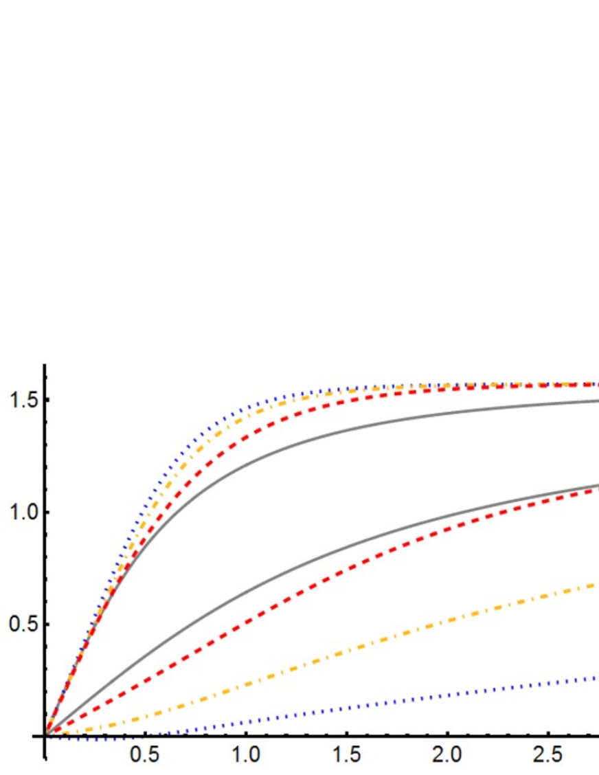
In Fig. 4, we display some set of numerical solutions for different values of the coupling at and their topological charge density defined through . The solutions enjoy Derrick’s scaling relation and possess a good approximated value of the topological charge, as shown in Table 1. One observes that as the value of the coupling becomes relatively small, the function is delocalizing while the profile function is approaching its vacuum value everywhere in space except for the origin. This is an indication that any regular non-trivial solution does not exist .
4.2 Asymptotic behavior
Asymptotic interaction of solitons is related to the overlapping of the tails of the profile functions of well-separated single solitons [3]. Bounded multi-soliton configurations may exist if there is an attractive force between two isolated solitons.
Considering the above-mentioned soliton solutions of the gauged NL-model, we have seen that the exact solution (4.2) has the same type of asymptotic decay as any solution of the general system (4.8). Therefore, it is enough to examine the asymptotic force between the solutions on the solvable line (4.2) to understand whether or not the Hamiltonian (3.30) supports multi-soliton solutions of higher topological degrees. Thus, without loss of generality, we can set .
Following the approach discussed in Ref. [3], let us consider a superposition of two exact solutions above. This superposition is no longer a solution of the Euler-Lagrange equation, except for in the limit of infinite separation, because there is a force acting on the solitons. The interaction energy of two solitons can be written as
| (4.22) |
where is the energy of two BPS solitons separated by some large but finite distance from each other, and stands for the static energy of a single exact solution. Notice that the lower bound of the Hamiltonian (3.30) with is given
| (4.23) |
where the equality is enjoyed only by holomorphic solutions. Therefore, we immediately conclude
| (4.24) |
where the equality is satisfied only at the limit . It follows that the interaction energy is always positive for finite separation, and the interaction is repulsive. Since the exact solution has the topological charge , it implies that there are no isolated soliton solutions with the topological charge in this model. Note that, however, as the BPS solution (3.19) suggests, there can exist soliton solutions with an arbitrary negative charge, which are topological excited states on top of the homogeneous vacuum state.
5 Conclusion
In this paper, we have studied two-dimensional Skyrmions in the NL-model with a Lifshitz invariant term which is an generalization of the DM term. We have shown that the tilted FM Heisenberg model turns out to be an gauged NL-model in which the term linear in a background gauge field can be viewed as a Lifshitz invariant. We have found exact BPS-type solutions of the gauged model in the presence of a potential term with a specific value of the coupling constant. The least energy configuration among the BPS solutions has been discussed. We have reduced the gauged model to the (ungauged) model with a Lifshitz invariant by choosing a background gauge field. In the reduced model, we have constructed an exact solution for a special combination of coupling constants called the solvable line and numerical solutions for a wider range of them.
For numerical study, we chose the background field, generating a potential term that can be interpreted as the quadratic Zeeman term or uniaxial anisotropic term. One can also choose a background field generating the Zeeman term; if the background field is chosen as and , the associated potential term is proportional to . The Euler-Lagrange equation for the extended model with this background field is not compatible with the axial symmetric ansatz (4.1). Therefore, a two-dimensional full simulation is required to obtain a solution with this background field. This problem, numerical simulation for non-axial symmetric solutions in the model with a Lifshitz invariant, is left to future study. In addition, the construction of a Skyrmion lattice is a challenging problem. The physical interpretation of the Lifshitz invariants is also an important future task. The microscopic derivation of the tilted Heisenberg model [21] may enable us to understand the physical interpretation and physical situation where the Lifshitz invariant appears. Other future work would be the extension of the present study to the antiferromagnetic Heisenberg model where soliton/sphaleron solutions can be constructed [41, 42, 43].
We restricted our analysis on the case that the additional potential term is balanced or dominant against the anisotropic potential term , i.e., . We expect that a classical phase transition occurs outside of the condition, and it causes instability of the solution. At the moment, the phase structure of the model (3.30) is not clear, and we will discuss it in our subsequent work.
Moreover, it has been reported that in some limit of a three-component Ginzburg-Landau model [44, 45], and of a three-component Gross-Pitaevskii model [46, 47], their vortex solutions can be well-described by planar Skyrmions. We believe that our result provides a hint to introduce a Lifshitz invariant to the models, and that our solutions find applications not only in spin systems but also in superconductors and Bose-Einstein condensates described by the extended models, including the Lifshitz invariant.
Acknowledgments
This work was supported by JSPS KAKENHI Grant Nos. JP17K14352, JP20K14411, and JSPS Grant-in-Aid for Scientific Research on Innovative Areas “Quantum Liquid Crystals” (KAKENHI Grant No. JP20H05154). Ya.S. gratefully acknowledges support by the Ministry of Education of Russian Federation, project FEWF-2020-0003.
Y. Amari would like to thank Tokyo University of Science for its kind hospitality.
References
- [1] T. Skyrme, “A Nonlinear field theory”, Proc. Roy. Soc. Lond. A 260, 127–138 (1961) .
- [2] T. Skyrme, “A Unified Field Theory of Mesons and Baryons”, Nucl. Phys. 31, 556–569 (1962) .
- [3] N. Manton, and P. Sutcliffe, “Topological solitons”, Cambridge Monographs on Mathematical Physics, Cambridge University Press, 2004.
- [4] A. Bogolubskaya, and I. Bogolubsky, “Stationary Topological Solitons in the Two-dimensional Anisotropic Heisenberg Model With a Skyrme Term”, Phys. Lett. A 136, 485–488 (1989) .
- [5] A. Bogolyubskaya, and I. Bogolyubsky, “ON STATIONARY TOPOLOGICAL SOLITONS IN TWO-DIMENSIONAL ANISOTROPIC HEISENBERG MODEL”, Lett. Math. Phys. 19, 171–177 (1990) .
- [6] R. A. Leese, M. Peyrard, and W. J. Zakrzewski, “Soliton Scatterings in Some Relativistic Models in (2+1)-dimensions”, Nonlinearity 3, 773–808 (1990) .
- [7] A. M. Polyakov, and A. Belavin, “Metastable States of Two-Dimensional Isotropic Ferromagnets”, JETP Lett. 22, 245–248 (1975) .
- [8] A. N. Bogdanov, and D. Yablonskii, “Thermodynamically stable “vortices” in magnetically ordered crystals. The mixed state of magnets”, Zh. Eksp. Teor. Fiz 95 (1), 178 (1989) .
- [9] A. Neubauer, C. Pfleiderer, B. Binz, A. Rosch, R. Ritz, P. Niklowitz, and P. Böni, “Topological Hall effect in the A phase of MnSi”, Phys. Rev. Lett. 102 (18), 186602 (2009) .
- [10] N. Nagaosa, and Y. Tokura, “Topological properties and dynamics of magnetic skyrmions”, Nat. Nanotechnol. 8 (12), 899–911 (2013) .
- [11] A. Leonov, I. Dragunov, U. Rößler, and A. Bogdanov, “Theory of skyrmion states in liquid crystals”, Phys. Rev. E 90 (4), 042502 (2014) .
- [12] I. I. Smalyukh, Y. Lansac, N. A. Clark, and R. P. Trivedi, “Three-dimensional structure and multistable optical switching of triple-twisted particle-like excitations in anisotropic fluids”, Nat. Mater. 9 (2), 139–145 (2010) .
- [13] S. Mühlbauer, B. Binz, F. Jonietz, C. Pfleiderer, A. Rosch, A. Neubauer, R. Georgii, and P. Böni, “Skyrmion lattice in a chiral magnet”, Science 323 (5916), 915–919 (2009) .
- [14] X. Yu, Y. Onose, N. Kanazawa, J. Park, J. Han, Y. Matsui, N. Nagaosa, and Y. Tokura, “Real-space observation of a two-dimensional skyrmion crystal”, Nature 465 (7300), 901–904 (2010) .
- [15] S. Heinze, K. Von Bergmann, M. Menzel, J. Brede, A. Kubetzka, R. Wiesendanger, G. Bihlmayer, and S. Blügel, “Spontaneous atomic-scale magnetic skyrmion lattice in two dimensions”, Nat. Phys. 7 (9), 713–718 (2011) .
- [16] C. Back, V. Cros, H. Ebert, K. Everschor-Sitte, A. Fert, M. Garst, T. Ma, S. Mankovsky, T. L. Monchesky, M. Mostovoy, N. Nagaosa, S. S. P. Parkin, C. Pfleiderer, N. Reyren, A. Rosch, Y. Taguchi, Y. Tokura, K. von Bergmann, and J. Zang, “The 2020 skyrmionics roadmap”, J. Phys. D: Appl. Phys. 53 (36), 363001 (2020) .
- [17] I. Dzyaloshinsky, “A thermodynamic theory of “weak” ferromagnetism of antiferromagnetics”, J. Phys. Chem. Solids 4 (4), 241–255 (1958) .
- [18] T. Moriya, “Anisotropic superexchange interaction and weak ferromagnetism”, Physical review 120 (1), 91 (1960) .
- [19] Y.-Q. Li, Y.-H. Liu, and Y. Zhou, “General spin-order theory via gauge Landau-Lifshitz equation”, Phys. Rev. B 84 (20), 205123 (2011) .
- [20] B. J. Schroers, “Gauged Sigma Models and Magnetic Skyrmions”, SciPost Phys. 7 (3), 030 (2019) .
- [21] S. Zhu, Y.-Q. Li, and C. D. Batista, “Spin-orbit coupling and electronic charge effects in Mott insulators”, Phys. Rev. B 90 (19), 195107 (2014) .
- [22] A. Sparavigna, “Role of Lifshitz invariants in liquid crystals”, Materials 2 (2), 674–698 (2009) .
- [23] P. Yudin, and A. Tagantsev, “Fundamentals of flexoelectricity in solids”, Nanotechnology 24 (43), 432001 (2013) .
- [24] B. Barton-Singer, C. Ross, and B. J. Schroers, “Magnetic Skyrmions at Critical Coupling”, Commun. Math. Phys. 375 (3), 2259–2280 (2020) .
- [25] C. Ross, N. Sakai, and M. Nitta, “Skyrmion Interactions and Lattices in Solvable Chiral Magnets”arXiv:2003.07147.
- [26] V. Golo, and A. Perelomov, “Solution of the Duality Equations for the Two-Dimensional SU(N) Invariant Chiral Model”, Phys. Lett. B 79, 112–113 (1978) .
- [27] A. D’Adda, M. Luscher, and P. Di Vecchia, “A 1/n Expandable Series of Nonlinear Sigma Models with Instantons”, Nucl. Phys. B 146, 63–76 (1978) .
- [28] A. Din, and W. Zakrzewski, “General Classical Solutions in the CP(n-1) Model”, Nucl. Phys. B 174, 397–406 (1980) .
- [29] L. Ferreira, and P. Klimas, “Exact vortex solutions in a Skyrme-Faddeev type model”, JHEP 10, 008 (2010) .
- [30] Y. Amari, P. Klimas, N. Sawado, and Y. Tamaki, “Potentials and the vortex solutions in the Skyrme-Faddeev model”, Phys. Rev. D 92 (4), 045007 (2015) .
- [31] B. Ivanov, R. Khymyn, and A. Kolezhuk, “Pairing of Solitons in Two-Dimensional S=1 Magnets”, Phys. Rev. Lett. 100 (4), 047203 (2008) .
- [32] A. Smerald, and N. Shannon, “Theory of spin excitations in a quantum spin-nematic state”, Phys. Rev. B 88, 184430 (2013) .
- [33] R. Hernandez, and E. Lopez, “The SU(3) spin chain sigma model and string theory”, JHEP 2004 (04), 052 (2004) .
- [34] M. Greiter, S. Rachel, and D. Schuricht, “Exact results for SU(3) spin chains: Trimer states, valence bond solids, and their parent Hamiltonians”, Phys. Rev. B 75 (6), 060401 (2007) .
- [35] K. Penc, and A. M. Läuchli, “Spin nematic phases in quantum spin systems”, in: Introduction to Frustrated Magnetism, Springer, 2011, pp. 331–362.
- [36] B. A. Ivanov, and A. K. Kolezhuk, “Effective field theory for the S=1quantum nematic”, Phys. Rev. B 68 (5).
- [37] K.-I. Kondo, S. Kato, A. Shibata, and T. Shinohara, “Quark confinement: Dual superconductor picture based on a non-Abelian Stokes theorem and reformulations of Yang–Mills theory”, Phys. Rept. 579, 1–226 (2015) .
- [38] W. J. Zakrzewski, “Low dimensional sigma models”, Hilger, 1989.
- [39] B. Piette, B. Schroers, and W. Zakrzewski, “Multi-solitons in a two-dimensional Skyrme model”, Z. Phys. C 65, 165–174 (1995) .
- [40] L. Döring, and C. Melcher, “Compactness results for static and dynamic chiral skyrmions near the conformal limit”, Calc. Var. Partial Differ. Equ. 56 (3), 60 (2017) .
- [41] D. Bykov, “Classical solutions of a flag manifold -model”, Nucl. Phys. B 902, 292–301 (2016) .
- [42] H. T. Ueda, Y. Akagi, and N. Shannon, “Quantum solitons with emergent interactions in a model of cold atoms on the triangular lattice”, Phys. Rev. A 93, 021606(R) (2016) .
- [43] Y. Amari, and N. Sawado, “BPS sphalerons in the nonlinear sigma model”, Phys. Rev. D 97, 065012 (2018) .
- [44] J. Garaud, J. Carlstrom, and E. Babaev, “Topological solitons in three-band superconductors with broken time reversal symmetry”, Phys. Rev. Lett. 107, 197001 (2011) .
- [45] J. Garaud, J. Carlström, E. Babaev, and M. Speight, “Chiral skyrmions in three-band superconductors”, Phys. Rev. B 87 (1), 014507 (2013) .
- [46] M. Eto, and M. Nitta, “Vortex trimer in three-component Bose-Einstein condensates”, Phys. Rev. A 85, 053645 (2012) .
- [47] M. Eto, and M. Nitta, “Vortex graphs as N-omers and CP(N-1) Skyrmions in N-component Bose-Einstein condensates”, EPL 103 (6), 60006 (2013) .