Iterated Schrödinger bridge approximation
to Wasserstein Gradient Flows

Let $\mathcal{P}_{2}(\mathbb{R}^{d})$ denote the space of square-integrable Borel probability measures on $\mathbb{R}^{d}$. Throughout this paper we will let $\rho\in\mathcal{P}_{2}(\mathbb{R}^{d})$ refer to both the measure and the its Lebesgue density, whenever it exists. $\mathcal{P}_{2}(\mathbb{R}^{d})$ can be turned into a metric space equipped with the Wasserstein-$2$ metric [AGS08, Chapter 7]. We will refer to this metric space as simply the Wasserstein space. For any pair of probability measures $(\rho_{1},\rho_{2})$ in the Wasserstein space, let $\Pi(\rho_{1},\rho_{2})$ denote the set of couplings, i.e., joint distributions, with marginals $(\rho_{1},\rho_{2})$. Further, define the relative entropy, also known as Kullback-Leibler (KL) divergence, between $\rho_{1}$ and $\rho_{2}$ as

To understand our results let us start with an example that was first described in [SABP22]. The static Schrödinger bridge ([Léo14]) at temperature $\varepsilon$ with both marginals $\rho$ is the solution to the following optimization problem

where $\mu_{\rho,\varepsilon}\in\mathcal{P}(\mathbb{R}^{d}\times\mathbb{R}^{d})$ has density

If $(X,Y)\sim\pi_{\rho,\varepsilon}{}$, define the barycentric projection [PNW22] as a function from $\mathbb{R}^{d}$ to itself given by

Now define a map from $\mathcal{P}_{2}(\mathbb{R}^{d})$ to itself given by the following pushforward

We call this map $\text{SB}_{\varepsilon}(\cdot)$ to emphasize the central role of the Schrödinger bridge in its definition. That is, if $(X,Y)\sim\pi_{\rho,\varepsilon}$, then $\text{SB}_{\varepsilon}(\rho)$ is the law of the random variable $2X-\mathrm{E}_{\pi_{\rho,\varepsilon}{}}[Y|X]$. If $\varepsilon\approx 0$, then $\pi_{\rho,\varepsilon}{}$ should closely approximate the quadratic cost optimal transport plan from $\rho$ to itself [Léo12]. That is, one would expect $\mathrm{E}_{\pi_{\rho,\varepsilon}{}}[Y|X]$ to be approximately close to $X$ itself (see, for instance, [PNW22, Corollary 1]). Therefore, one expects $2X-\mathrm{E}_{\pi_{\rho,\varepsilon}{}}[Y|X]\approx X$, as well. Hence, the pushforward should not alter $\rho$ by much.

What happens if we iterate this map and rescale time with $\varepsilon$? That is, fix some $\rho_{0}\in\mathcal{P}_{2}(\mathbb{R}^{d})$ and a $T>0$. Let $N_{\varepsilon}=\lfloor T\varepsilon^{-1}\rfloor$. With $\rho_{0}^{\varepsilon}\mathrel{\mathop{\mathchar 58\relax}}=\rho_{0}$, define iteratively

Define a continuous time piecewise constant interpolant $\left(\rho^{\varepsilon}(t)=\rho^{\varepsilon}_{\lfloor t/\varepsilon\rfloor},\;t\in[0,T]\right)$. The question is whether, as $\varepsilon\rightarrow 0+$, this curve on the Wasserstein space has an absolutely continuous limit? If so, can we write down its characterizing continuity equation?

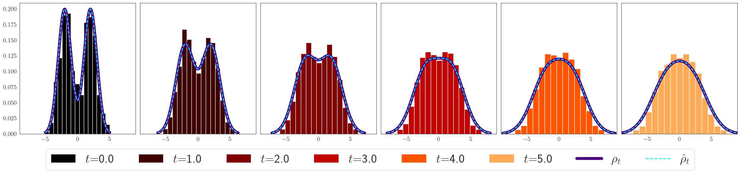
Before we give the answer, consider the simulation in Figure 1. The figure considers a particle system approximation to the above iterative scheme. We push $n=500$ particles, initially distributed as a mixtures of two normal distributions, $\rho_{0}\mathrel{\mathop{\mathchar 58\relax}}=0.5\,\mathcal{N}(-2,1)+0.5\,\mathcal{N}(2,1)$, via the dynamical system for $T=5$ and step size $\varepsilon=0.1$. At every step the Schrödinger bridge is approximated by the (matrix) Sinkhorn algorithm [Cut13] applied to the current empirical distribution of the particles and the corresponding barycenter is approximated from this estimate. The pushforward is then applied to the $n$ particles themselves. This gives a time evolving process of empirical distributions that can be thought of as a discrete approximation of our iterative scheme. One can see that the histogram gets smoothed out gradually and ends in a shape that appears to be a Gaussian distribution. In fact, this process of smoothing is reminiscent of the heat flow starting from $\rho_{0}$. In the case of this simple starting distribution, the heat flow $(\rho_{t},t\geq 0)$ is known analytically. The curves of the heat flow are superimposed as continuous curves. The broken curves are the exact $\rho^{\varepsilon}(\cdot)$ which, in this case, can also be computed. The histograms and the two curves all closely match with one another.

One of the results that we prove in this paper shows that, under appropriate assumptions, $\left(\rho^{\varepsilon}(t),\;t\in[0,T]\right)$ indeed converges to the solution of the heat equation $\frac{\partial}{\partial t}\rho_{t}=\frac{1}{2}\Delta\rho_{t}$, with initial condition $\rho_{0}$. In a different context and language, this result was first observed in [SABP22, Theorem 1]. However, their proof is incomplete. See the discussion below. The statement of Theorem 4 in this paper lays down sufficient conditions under which this convergence happens.

It is well known from [JKO98, Theorem 5.1] that the heat flow is the Wasserstein gradient flow of (one half) entropy. We prove a generalization of the above result where a similar discrete dynamical system converges, under assumptions, to other Wasserstein gradient flows that satisfy an evolutionary PDE of the type [AGS08, eqn. (11.1.6)]. The general existence and uniqueness of gradient flows (curves of maximal slopes) in Wasserstein space are quite subtle [AGS08, Chapter 11]. However, evolutionary PDEs of the type [AGS08, eqn. (11.1.6)] include the classical case of the gradient flow of entropy as the heat equation and that of the Kullback-Leibler divergence (also called relative entropy) as the Fokker-Planck equation [JKO98, Theorem 5.1]. Our iterative approximating schemes always iterate a function of the barycentric projection of the Schrödinger bridge with the same marginals. The marginal itself changes with the iteration. Let us give the reader an intuitive idea how such schemes work.

The foundations of all these results can be found in Theorem 1 which shows that the two point joint distribution of a stationary Langevin diffusion is a close approximation of the Schrödinger bridge with equal marginals. More concretely, let $\rho=e^{-g}$ be some element in $\mathcal{P}_{2}(\mathbb{R}^{d})$ for which the Langevin diffusion process with stationary distribution $\rho$ exists and is unique in law. This diffusion process is governed by the stochastic differential equation

where $(B_{t},t\geq 0)$ is the standard $d$-dimensional Brownian motion. Therefore, for any $\varepsilon>0$, $\ell_{\rho,\varepsilon}\mathrel{\mathop{\mathchar 58\relax}}=\text{Law}(X_{0},X_{\varepsilon})$ is an element in $\Pi(\rho,\rho)$. Then, Theorem 1 shows that, under appropriate conditions on $\rho$, the symmetrized relative entropy, i.e., the Jensen-Shannon divergence, between $\ell_{\rho,\varepsilon}$ and the Schrödinger bridge $\pi_{\rho,\varepsilon}$ is $o(\varepsilon^{2})$. Although this level of precision is sufficient for our purpose, it is shown via explicit computations in (28) that when $\rho$ is Gaussian this symmetrized relative entropy is actually $O(\varepsilon^{4})$, an order of magnitude tighter.

In any case, one would expect that, under suitable assumptions, the barycentric projection

The quantity $\nabla\log\rho$ is called the score function. This is a reformulation of [SABP22, Theorem 1] which states that the difference between the two sides converges to zero in $L^{2}(\rho)$. In other words, one would expect that, under suitable assumptions,

We claim this is approximately the solution of the heat equation at time $\epsilon$, starting from $\rho$.

To see this, recall that absolutely continuous curves (see [AGS08, Definition 1.1.1]) $\left(\rho_{t},\;t\geq 0\right)$ on the Wasserstein space are characterized as weak solutions [AGS08, eqn. (8.1.4)] of continuity equations

Here $v_{t}\mathrel{\mathop{\mathchar 58\relax}}\mathbb{R}^{d}\to\mathbb{R}^{d}$ is the time-dependent Borel velocity field of the continuity equation whose properties are given by [AGS08, Theorem 8.3.1]. For any absolutely continuous curve, if $v_{t}$ belongs to the tangent space at $\rho_{t}$ ([AGS08, Definition 8.4.1]), [AGS08, Proposition 8.4.6] states the following approximation result for Lebesgue-a.e. $t\geq 0$

For example, if $\rho$ is the Wasserstein gradient flow of a function $\mathcal{F}\mathrel{\mathop{\mathchar 58\relax}}\mathcal{P}_{2}(\mathbb{R}^{d})\to(-\infty,\infty]$ satisfying [AGS08, eqn. (11.1.6)], $v_{t}=-\nabla\frac{\delta\mathcal{F}}{\delta\rho_{t}}$ where $\frac{\delta\mathcal{F}}{\delta\rho_{t}}$ is the first variation of $\mathcal{F}$ (see [AGS08, Section 10.4.1]) at $\rho_{t}$. For the heat flow, which is the gradient flow of (half) entropy, $\frac{\delta\mathcal{F}}{\delta\rho_{t}}=\frac{1}{2}\log\rho_{t}$ and $v_{t}=-\frac{1}{2}\nabla\log\rho_{t}$. Comparing (8) with (10) explains the previous claim.

The claimed approximation in (8) is what we call one-step approximation. In a somewhat more general setting, this is proved in Theorem 2. Note that a crucial advantage we gain in the Schrödinger bridge scheme that is absent in Langevin diffusion or the continuity equation is that we no longer need to compute the score function $\nabla\log\rho$. Instead it suffices to be able to draw samples from $\rho$ and compute the approximate Schrödinger bridge, say by the Sinkhorn algorithm [Cut13], as done in Figure 1.

To summarize, the flow of ideas in the paper goes as follows. First, we show that the Schrödinger bridge map $\text{SB}_{\varepsilon}(\rho)$, defined in its full generality in (SB), is an approximation the pushforward of $\rho$ by the tangent vector of the gradient flow (10). This is known to be close to the gradient flow curve itself [AGS08, Proposition 8.4.6]. So one may expect that an iteration of this idea, where an absolutely continuous curve approximated by iterated pushforwards such as (10) can be, under suitable assumptions, approximated by iterated Schrödinger bridge operators $\text{SB}_{\varepsilon}(\cdot)$. One has to be mindful that the cumulative error remains controlled as we iterate, but in the best of situations this might work. And, in fact, it does for the heat flow, under suitable conditions, as proved in Theorem 4.

Now, a natural question is how general is this method? Can we approximate other gradient flows, say that of Kullback-Leibler with respect to a log-concave density? What about absolutely continuous curves that are not gradient flows? The case of KL is partially settled in this paper in Theorem 5. Let us state our proposed Schrödinger Bridge scheme in somewhat general notation. Consider a suitably nice functional $\mathcal{F}\mathrel{\mathop{\mathchar 58\relax}}\mathcal{P}_{2}(\mathbb{R}^{d})\to\mathbb{R}\cup\{+\infty\}$ and fix an initial measure $\rho_{0}\in\mathcal{P}_{2}(\mathbb{R}^{d})$. Suppose the gradient flow of $\mathcal{F}$ can be approximated by a sequence of explicit Euler iterations $\left(\tilde{\rho}_{\varepsilon}(k),\;k\in\mathbb{N}\right)$, where, starting from $\tilde{\rho}_{\varepsilon}(0)=\rho_{0}$, iteratively define

with $-\nabla u_{k-1}$ being the Wasserstein gradient of $\mathcal{F}$ at $\tilde{\rho}_{\varepsilon}(k-1)$. Such an approximation scheme will be referred to as an explicit Euler iteration scheme and conditions must be imposed for it to converge to the underlying gradient flow. See Theorem 3 below for sufficient conditions.

Ignoring technical details, our goal is to approximate each such explicit Euler step via a corresponding Schrödinger bridge step. This is accomplished by the introduction of what we call a surrogate measure. For simplicity, consider the first step $\tilde{\rho}_{\varepsilon}(1)=\left(\operatorname{\mathrm{Id}}+\varepsilon\nabla u_{0}\right)_{\#}\rho_{0}$. Suppose that there is some $\theta\in\mathbb{R}\setminus\{0\}$ such that $\int e^{2\theta u_{0}}<\infty$, define the surrogate measure $\sigma_{0}$ to be one with the density

As explained in (7), if we consider the Schrödinger bridge at temperature $\varepsilon$ with both marginals to be $\sigma_{0}$, then $\mathcal{B}_{\sigma_{0},\varepsilon}(x)\approx x+\frac{\varepsilon}{2}\nabla\log\sigma_{0}(x)=x+\theta\varepsilon\nabla u_{0}(x)$. If we now define one step in the SB scheme as

Observing that, as $\varepsilon\downarrow 0$, we recover that $\text{SB}_{\varepsilon}(\rho)\approx(\operatorname{\mathrm{Id}}+\varepsilon\nabla u_{0})_{\#}\rho$. Notice that the choice of $\theta$ does not play a role except to guarantee that the surrogate $\sigma_{0}$ in (12) is integrable. For the case of the heat flow, $u_{0}=-\frac{1}{2}\log\rho_{0}$. Hence, if we pick $\theta=-1$, $\sigma_{0}=\rho_{0}$ and then the scheme (5) becomes a special case of (SB).

Let us consider the sequence of iterates of (SB), interpolated in continuous time for some $0<T<\infty$,

Theorems 4 and 5 list sufficient conditions under which such a scheme converges uniformly to the gradient flow curve as $\varepsilon\rightarrow 0+$ for specific choices of functional $\mathcal{F}$.

We should point out that the primary reason why we need the assumptions in Theorems 4 and 5 is to guarantee that the errors go to zero uniformly over a growing number of iterations. Much of the technical work in this paper goes to produce a simple set of sufficient conditions to ensure this. Consequently, our theorems are specialized to the case of gradient flows of geodesically convex regular functions. But the scope of Schrödinger bridge scheme is potentially larger. As shown in Section 5.3 via explicit calculations, the Schrödinger bridge scheme may be used to approximate even time-reversed gradient flows. The corresponding PDEs, such as the backward heat equation/ Fokker-Planck, are ill-posed and care must be taken to implement any approximating scheme. Interestingly, if one replaces (5) by $\text{SB}_{\varepsilon}(\rho)\mathrel{\mathop{\mathchar 58\relax}}=\left(\mathcal{B}_{\rho,\varepsilon}\right)_{\#}\rho$, then starting from a Gaussian initial distribution, and for all small enough $\varepsilon$, the iterates are shown to converge to the time-reversed gradient flow of one-half entropy.

In Section 3 we also generalize our Schrödinger bridge scheme (SB) by picking the surrogate measure depending on $\varepsilon$. This generalization is necessary to generalize the Schrödinger bridge scheme to cover tangent vectors that are not necessarily of the gradient type, but are approximated by a sequence of gradient fields. This generalization also covers the case of the renowned JKO scheme, [JKO98], which can be likened to the implicit Euler discretization scheme of the gradient flow curve. This, however, introduces an additional layer of complexity.

Some of the technical challenges we overcome in this paper involve proving results about Schrödinger bridges at low temperatures when the marginals are not compactly supported. The latter is a common assumption in the literature, see for example [Pal19, PNW22, CCGT22, SABP22]. However, the existence of Langevin diffusion requires an unbounded support. Much of this work is done in Section 2 which may be of independent interest. For example, we extend the expansion of entropic OT cost function from [CT21, Theorem 1.6] for the case of same marginals in (42). In all this analysis an unexpected mathematical object appears repeatedly, the harmonic characteristic ([CVR18]) defined below in (14). It appears in the computation of Fisher information of the Langevin and the Schrödinger bridges (see (37)) and in the geodesic approximation of the heat flow (Lemma 7). The role of this object merits a deeper study.

Discussion on [SABP22]. The inspiring work [SABP22] is one of the motivations of our investigations. The authors of [SABP22] propose and analyze a modification to the self-attention mechanism from the Transformer artificial neural network architecture in which the self-attention matrix is enforced to be doubly-stochastic. Since the Sinkhorn algorithm is applied to enforce double stochasticity, the architecture is called the Sinkformer. A major contribution of [SABP22] is the keen observation that self-attention mechanisms can be understood as determining a dynamical system whose particles are the input tokens (possibly after a suitable transformation). See also [GLPR24] for other work in this area. Specifically, [SABP22, Proposition 2,3] observes that, as a regularization parameter vanishes, the associated particle system under doubly-stochastic self-attention evolves according to the heat flow, and this property naturally follows from the doubly-stochastic constraints.

Theorems 1-5 can be understood as probabilistic approaches to [SABP22, Theorem 1], as well as a finer treatment to key steps of the mathematical analysis of the convergence to the heat flow equation. The first statement of [SABP22, Theorem 1] concerns the convergence of the rescaled gradients of entropic potentials for the Schrödinger bridge with the same marginals. Consider the so-called entropic (or, Schrödinger) potentials $(f_{\varepsilon},\varepsilon>0)$ as defined later on in (19). In this language, [SABP22, Theorem 1] states that $\varepsilon^{-1}\nabla f_{\varepsilon}\to-\nabla\log\rho$ in $L^{2}(\rho)$, as $\varepsilon\rightarrow 0+$. We are not able to prove this particular convergence; not least because we work in a slightly different setting, i.e., with measures fully supported on $\mathbb{R}^{d}$ whereas [SABP22] assumes compact support (although, see the discussion after the proof of Theorem 1 for a similar result). Instead our argument relies on approximating the Schrödinger bridge by the Langevin diffusion which are undefined for measures with compact support. Moreover, in our paper we develop a general machinery that demonstrate the ability of the Schrödinger bridge scheme to approximate gradient flows of other functionals of interest beyond entropy.

References

• [AGS08] Luigi Ambrosio, Nicola Gigli, and Giuseppe Savaré. Gradient flows in metric spaces and in the space of probability measures. Lectures in Mathematics ETH Zürich. Birkhäuser Verlag, Basel, second edition, 2008.
• [BGL14] Dominique Bakry, Ivan Gentil, and Michel Ledoux. Analysis and geometry of Markov diffusion operators, volume 348 of Grundlehren der mathematischen Wissenschaften [Fundamental Principles of Mathematical Sciences]. Springer, Cham, 2014.
• [BGN22] Espen Bernton, Promit Ghosal, and Marcel Nutz. Entropic optimal transport: geometry and large deviations. Duke Math. J., 171(16):3363–3400, 2022.
• [Bob22] Sergey G. Bobkov. Upper bounds for Fisher information. Electron. J. Probab., 27:Paper No. 115, 44, 2022.
• [CCGT22] Alberto Chiarini, Giovanni Conforti, Giacomo Greco, and Luca Tamanini. Gradient estimates for the schrödinger potentials: convergence to the brenier map and quantitative stability, 2022.
• [CG14] P. Cattiaux and A. Guillin. Semi log-concave Markov diffusions. In Séminaire de Probabilités XLVI, volume 2123 of Lecture Notes in Math., pages 231–292. Springer, Cham, 2014.
• [Csi75] I. Csiszár. II-divergence geometry of probability distributions and minimization problems. Ann. Probability, 3:146–158, 1975.
• [CT21] Giovanni Conforti and Luca Tamanini. A formula for the time derivative of the entropic cost and applications. J. Funct. Anal., 280(11):Paper No. 108964, 48, 2021.
• [Cut13] Marco Cuturi. Sinkhorn distances: Lightspeed computation of optimal transport. Advances in neural information processing systems, 26, 2013.
• [CVR18] Giovanni Conforti and Max Von Renesse. Couplings, gradient estimates and logarithmic Sobolev inequality for Langevin bridges. Probab. Theory Related Fields, 172(1-2):493–524, 2018.
• [DGW04] H. Djellout, A. Guillin, and H. Wu. Transportation cost-information inequalities and applications to random dynamical systems and diffusions. Ann. Probab., 32(3B):2702–2732, 2004.
• [GLPR24] Borjan Geshkovski, Cyril Letrouit, Yury Polyanskiy, and Philippe Rigollet. The emergence of clusters in self-attention dynamics. Arxiv preprint 2305.05465, 2024.
• [GLR17] Ivan Gentil, Christian Léonard, and Luigia Ripani. About the analogy between optimal transport and minimal entropy. Ann. Fac. Sci. Toulouse Math. (6), 26(3):569–601, 2017.
• [GLRT20] Ivan Gentil, Christian Léonard, Luigia Ripani, and Luca Tamanini. An entropic interpolation proof of the HWI inequality. Stochastic Process. Appl., 130(2):907–923, 2020.
• [JKO98] Richard Jordan, David Kinderlehrer, and Felix Otto. The variational formulation of the Fokker-Planck equation. SIAM J. Math. Anal., 29(1):1–17, 1998.
• [JMPC20] Hicham Janati, Boris Muzellec, Gabriel Peyré, and Marco Cuturi. Entropic optimal transport between unbalanced Gaussian measures has a closed form. NIPS’20, Red Hook, NY, USA, 2020. Curran Associates Inc.
• [KS91] Ioannis Karatzas and Steven E. Shreve. Brownian motion and stochastic calculus, volume 113 of Graduate Texts in Mathematics. Springer-Verlag, New York, second edition, 1991.
• [Léo12] Christian Léonard. From the Schrödinger problem to the Monge-Kantorovich problem. J. Funct. Anal., 262(4):1879–1920, 2012.
• [Léo14] Christian Léonard. A survey of the Schrödinger problem and some of its connections with optimal transport. Discrete Contin. Dyn. Syst., 34(4):1533–1574, 2014.
• [LK93] B. C. Levy and A. J. Krener. Dynamics and kinematics of reciprocal diffusions. Journal of mathematical physics, 34(5):1846–1875, 1993.
• [LYB+24] Sungbin Lim, Eun Bi Yoon, Taehyun Byun, Taewon Kang, Seungwoo Kim, Kyungjae Lee, and Sungjoon Choi. Score-based generative modeling through stochastic evolution equations in Hilbert spaces. Advances in Neural Information Processing Systems, 36, 2024.
• [Olv13] P.J. Olver. Introduction to Partial Differential Equations. Undergraduate Texts in Mathematics. Springer International Publishing, 2013.
• [Pal19] Soumik Pal. On the difference between entropic cost and the optimal transport cost, 2019. Arxiv 1905.12206. To appear in The Annals of Applied Probability.
• [PNW22] Aram-Alexandre Pooladian and Jonathan Niles-Weed. Entropic estimation of optimal transport maps, 2022.
• [Roy07] Gilles Royer. An initiation to logarithmic Sobolev inequalities, volume 14 of SMF/AMS Texts and Monographs. American Mathematical Society, Providence, RI; Société Mathématique de France, Paris, 2007. Translated from the 1999 French original by Donald Babbitt.
• [RY04] D. Revuz and M. Yor. Continuous Martingales and Brownian Motion. Grundlehren der mathematischen Wissenschaften. Springer Berlin Heidelberg, 2004.
• [SABP22] Michael E. Sander, Pierre Ablin, Mathieu Blondel, and Gabriel Peyré. Sinkformers: Transformers with doubly stochastic attention. In Gustau Camps-Valls, Francisco J. R. Ruiz, and Isabel Valera, editors, Proceedings of The 25th International Conference on Artificial Intelligence and Statistics, volume 151 of Proceedings of Machine Learning Research, pages 3515–3530. PMLR, 28–30 Mar 2022.
• [San15] Filippo Santambrogio. Optimal transport for applied mathematicians: Calculus of variations, PDEs, and modeling, volume 87. Springer, 2015.
• [SSDK+20] Yang Song, Jascha Sohl-Dickstein, Diederik P Kingma, Abhishek Kumar, Stefano Ermon, and Ben Poole. Score-based generative modeling through stochastic differential equations. In International Conference on Learning Representations, 2020. ArXiv version 2011.13456.
• [Ver18] Roman Vershynin. High-dimensional probability, volume 47 of Cambridge Series in Statistical and Probabilistic Mathematics. Cambridge University Press, Cambridge, 2018. An introduction with applications in data science, With a foreword by Sara van de Geer.
• [Vil03] Cédric Villani. Topics in optimal transportation, volume 58. American Mathematical Soc., 2003.
Notations
Symbol Explanation
Cd[0,)C^{d}[0,\infty) Collection of continuous paths ω:[0,)d\omega\mathrel{\mathop{\mathchar 58\relax}}[0,\infty)\to\mathbb{R}^{d}
Ck(d)C^{k}(\mathbb{R}^{d}) kk-times continuously differentiable functions d\mathbb{R}^{d}\to\mathbb{R}
𝒫2(d)\mathcal{P}_{2}(\mathbb{R}^{d}) Space of twice integrable probability measures on d\mathbb{R}^{d}
𝒫2ac(d)\mathcal{P}_{2}^{ac}(\mathbb{R}^{d}) Space of twice integrable and absolutely continuous probability measures (with respect to Lebesgue measure) on d\mathbb{R}^{d}
Cc(d)C_{c}^{\infty}(\mathbb{R}^{d}) Space of smooth and compactly supported functions in d\mathbb{R}^{d}
𝕎2(μ,ν)\mathbb{W}_{2}(\mu,\nu) Wasserstein-2 distance between measures μ\mu and ν\nu in 𝒫2(d)\mathcal{P}_{2}(\mathbb{R}^{d})
TμνT_{\mu}^{\nu} Optimal transport map from μ\mu to ν\nu (if it exists)
(πt,t0)(\pi_{t},t\geq 0) Coordinatewise projections on Cd[0,)C^{d}[0,\infty), πs(ω)=ωs\pi_{s}(\omega)=\omega_{s}
μρ,ε\mu_{\rho,\varepsilon} μρ,ε(dx,dy)=(2πε)d/2ρ(x)exp(xy2/2ε)dxdy\mu_{\rho,\varepsilon}(dx,dy)=(2\pi\varepsilon)^{-d/2}\rho(x)\exp\left(-\|x-y\|^{2}/2\varepsilon\right)dxdy
(Wx,xd)(W_{x},x\in\mathbb{R}^{d}) Wiener measure on Cd[0,)C^{d}[0,\infty) with initial condition δx\delta_{x}
WW Reversible Wiener measure on Cd[0,)C^{d}[0,\infty)
RεR_{\varepsilon} Law of reversible Brownian motion with diffusion ε\varepsilon
(Pt,t0)(P_{t},t\geq 0) Brownian semigroup
(pt(,),t>0)(p_{t}(\cdot,\cdot),t>0) Brownian transition densities
QQ Law of stationary Langevin diffusion on Cd[0,)C^{d}[0,\infty)
ρ,ε\ell_{\rho,\varepsilon} Joint law of Langevin diffusion at time 0 and ε\varepsilon, i.e. (π0,πε)#Q(\pi_{0},\pi_{\varepsilon})_{\#}Q
(qt(,),t>0)(q_{t}(\cdot,\cdot),t>0) Transition densities for Langevin diffusion
LL Extended generator for the Langevin diffusion
(Gt,t0)(G_{t},t\geq 0) Langevin semigroup
πρ,ε\pi_{\rho,\varepsilon} ε\varepsilon-static Schrödinger bridge with marginals equal to ρ\rho
(fε,ε>0)(f_{\varepsilon},\varepsilon>0) Entropic potentials associated to (πρ,ε,ε>0)(\pi_{\rho,\varepsilon},\varepsilon>0)
ρ,ε\mathcal{B}_{\rho,\varepsilon} Barycentric projection associated with πρ,ε\pi_{\rho,\varepsilon}, ρ,ε(x)=Eπρ,ε[Y|X=x]\mathcal{B}_{\rho,\varepsilon}(x)=\mathrm{E}_{\pi_{\rho,\varepsilon}}[Y|X=x]
Sρ,εS_{\rho,\varepsilon} Law of ε\varepsilon-dynamic Schrödinger bridge on Cd[0,1]C^{d}[0,1] with initial and terminal distribution ρ\rho
(ρtε,t[0,1])(\rho_{t}^{\varepsilon},t\in[0,1]) Entropic interpolation from ρ\rho to itself, ρtε=(πt)#Sρ,ε\rho_{t}^{\varepsilon}=(\pi_{t})_{\#}S_{\rho,\varepsilon}
ψ1\|\cdot\|_{\psi_{1}} Subexponential norm of a random variable, [Ver18, Definition 2.7.5]
Tan(μ)\text{Tan}(\mu) Tangent bundle of 𝒫2(d)\mathcal{P}_{2}(\mathbb{R}^{d}) at μ\mu
Ent(μ)\mathrm{Ent}(\mu) Entropy of μ𝒫2ac(d)\mu\in\mathcal{P}_{2}^{ac}(\mathbb{R}^{d})
H(μ|ν)H(\mu|\nu) Kullback-Leibler divergence between μ\mu and ν\nu
I(ρ)I(\rho) Fisher information of ρ\rho, I(ρ)=Eρlogρ2I(\rho)=\mathrm{E}_{\rho}\|\nabla\log\rho\|^{2} for ρ𝒫2ac(d)\rho\in\mathcal{P}_{2}^{ac}(\mathbb{R}^{d})
SBεk(μ0)\text{SB}_{\varepsilon}^{k}(\mu_{0}) kkth iterate of Schrödinger bridge scheme starting from μ0\mu_{0} with stepsize ε\varepsilon
Sεk(μ0)S_{\varepsilon}^{k}\left(\mu_{0}\right) kkth iterate of pushforward of form (Id+εvε)#μ0(\operatorname{\mathrm{Id}}+\varepsilon v_{\varepsilon})_{\#}\mu_{0}, where each vε:ddv_{\varepsilon}\mathrel{\mathop{\mathchar 58\relax}}\mathbb{R}^{d}\to\mathbb{R}^{d} is a vector field specified in context