This paper was converted on www.awesomepapers.org from LaTeX by an anonymous user.
Want to know more? Visit the Converter page.

Iterative weak approximation and hard bounds for switching diffusion

Qinjing Qiu111Email address: qqiu9438@uni.sydney.edu.au. Postal Address: School of Mathematics and Statistics, University of Sydney, NSW 2006, Australia. TEL: +61(0)2-9114-1264 FAX: +61(0)2-9351-4534   and Reiichiro Kawai222Email address: raykawai@g.ecc.u-tokyo.ac.jp. Graduate School of Arts and Sciences / Mathematics and Informatics Center, The University of Tokyo, Tokyo 153-8902, Japan, and School of Mathematics and Statistics, The University of Sydney, NSW 2006, Australia. This work was partially supported by JSPS Grants-in-Aid for Scientific Research 20K22301 and 21K03347.
Abstract

We establish a novel convergent iteration framework for a weak approximation of general switching diffusion. The key theoretical basis of the proposed approach is a restriction of the maximum number of switching so as to untangle and compensate a challenging system of weakly coupled partial differential equations to a collection of independent partial differential equations, for which a variety of accurate and efficient numerical methods are available. Upper and lower bounding functions for the solutions are constructed using the iterative approximate solutions. We provide a rigorous convergence analysis for the iterative approximate solutions, as well as for the upper and lower bounding functions. Numerical results are provided to examine our theoretical findings and the effectiveness of the proposed framework.

Keywords: continuous-time Markov chains; diffusion processes; recursive iterations; hidden Markov model; weakly coupled partial differential equations.

2020 Mathematics Subject Classification: 60J27, 60H10, 60J22, 65C30

1 Introduction

Owing to the increasing demands on regime-switching diffusion from emerging applications in financial engineering and wireless communications, much attention has been given to switching diffusion processes. A salient feature of such systems is that they include both continuous dynamic and discrete events.

States of the environment process was referred to in [20] as economic circumstances or political regime-switching. It is therefore theoretically appealing to modify the classical diffusion process so that both expected return and the variance reflect the changes in the external environmental factors. The modelling framework that is advocated in this paper achieves this. The rationale is that in the different modes or regimes, the volatility and return rates can be very different. Another example is from a wireless communication networks. Consider the performance analysis of an adaptive, linear, multi-user detector in a cellular, direct-sequence, code-division, multiple-access wireless network with changing user activity due to an admission or access controller at the base station. Under certain conditions, an optimization problem for the aforementioned application leads to certain issues, which in turn lead to switching diffusion limit [26].

One early attempt at such hybrid models for financial applications can be traced back to the 1960s in which both the appreciation rate and the volatility of a stock depend on a continuous-time Markov chain. The introduction of such models makes it possible to describe stochastic volatility in a relatively simple manner. To illustrate, in the simplest case, a stock market may be considered to have two “modes” or “regimes”, up and down, resulting from the state of the underlying economy, the general mood of investors in the market, and so on. The primary motivation for the generalization is to enhance the flexibility of the model parameter settings for the classical diffusion process. The examples usually given are weather conditions and epidemic outbreaks, even though seasonality would play a role and can probably not be modelled by a Markov regime-switching model.

A variety of numerical methods extend those that already exist in the single-regime setting, but the extensions are rarely straightforward due to the inter-dependence nature of regime switching systems. Lattice methods in regime-switching settings have been attempted; first in [5] in a two-regime setting and later in the form of the adaptive mesh model [11], the 2k2k-branch lattice for a kk-regime model [1], and the trinomial method [28]. Mathematical programming is employed for obtaining hard bounds on regime-switching diffusion in [4, 19]. Approaches based on penalty methods for pricing American options have also been extended in a non-trivial way to regime-switching frameworks. For instance, in [14, 17, 18], exponential time difference schemes are applied in combination with a penalty method to approximate a solution to the complex system of partial differential equations with coupled free boundary conditions that arise in the presence of a regime-switching diffusion. The Fourier space time-stepping method [15] overcomes some of the problems encountered by lattice methods and finite-difference schemes when it comes to option pricing in models in higher dimensions or models containing jumps. This approach is applicable to a wide class of path-dependent options and options on multiple assets in regime-switching diffusion containing jumps.

A Monte Carlo method is presented in [13] for pricing barrier option in regime-switching diffusion, where the author demonstrates the non-trivial modifications that must be made in order to extend standard simulation-based techniques from the single-regime setting to multiple regimes. Esscher transform methods are employed in [9] and [10] for pricing European and American options in regime-switching diffusion and jump-diffusion settings. The Canadization method was extended to regime-switching settings to price American options [7] and double barrier options [6]. We mention the radial basis collocation method [3], a mesh-free method for pricing American options under regime-switching jump diffusion models. A MATLAB toolbox specially designed for the estimation, simulation and forecasting of a general Markov regime-switching diffusion is developed in [23]. In all the aforementioned studies, a great deal of special attention must be paid to the switching nature.

In this paper, we establish a novel convergent iteration framework on a generalized Feynman-Kac formula under regime-switching, which are the solutions to a set of weakly coupled partial differential equations with initial and boundary value conditions. We construct our recursive approximation mechanism by restricting the maximum number of switching occurring before the terminal time in the probabilistic representation in a similar manner to [24, 25]. The significance of the present approach is that it succeeds to untangle and compensate a challenging set of weakly coupled partial differential equations to a set of independent partial differential equations. Such untangling of the inter-dependency is quite remarkable, as undoubtedly a variety of accurate and efficient numerical methods are available for the latter untangled partial differential equations.

The rest of the paper is organized as follows. We present the necessary background materials and problem formulation regarding regime-switching diffusion in Section 2. We prove in Sections 3.1 and 3.2 that such an approximation can be obtained as the solution to a set of independent partial differential equations with additional heat source (the non-homogeneous terms) and additional discounting rates or, equivalently, the approximation admits a probabilistic representation under a probability measure without regime-switching. Further, in Section 3.3, we derive hard bounding functions for the true solution under regime-switching based on the approximation at each iteration as well as their convergence to the unknown solution. After briefly discussing the proposed approach in the context the initial-boundary value problem in Section 4, we examine our theoretical findings through numerical results in Section 5. Finally, Section 6 concludes the present study and highlights future research directions.

2 Preliminaries

We begin with the notation that will be used throughout the paper. We denote by \mathbb{R} the set of real numbers, and by :={1,2,}\mathbb{N}:=\{1,2,\cdots\} the set of natural numbers excluding 0, with 0:={0}\mathbb{N}_{0}:=\mathbb{N}\cup\{0\}. We reserve pp, nn and dd for fixed positive integers. We denote by {Rt:t0}\{R_{t}:t\geq 0\} a one-dimensional Markov process with right-continuous sample paths taking values in the finite-state space :={1,,p}\mathcal{M}:=\{1,\cdots,p\}. We define an nn-dimensional stochastic process {Xt:t0}\{X_{t}:t\geq 0\} taking values in a suitable domain D(n)D(\subseteq\mathbb{R}^{n}) by the stochastic differential equation:

dXt=b(t,Xt,Rt)dt+σ(t,Xt,Rt)dWt,(X0,R0)D×,dX_{t}=b(t,X_{t},R_{t})dt+\sigma(t,X_{t},R_{t})dW_{t},\quad(X_{0},R_{0})\in D\times\mathcal{M}, (2.1)

where {Wt:t0}\{W_{t}:t\geq 0\} is a dd-dimensional standard Brownian motion and the drift coefficient b:[0,)×D×nb:[0,\infty)\times D\times\mathcal{M}\to\mathbb{R}^{n} and the diffusion coefficient σ:[0,)×D×n×d\sigma:[0,\infty)\times D\times\mathcal{M}\to\mathbb{R}^{n\times d} are deterministic functions satisfying the usual conditions [12, 21]: for each ii\in\mathcal{M}, σ(,,i)\sigma(\cdot,\cdot,i) and b(,,i)b(\cdot,\cdot,i) are at most of linear growth and Lipschitz continuous on every compact subset of [0,)×D[0,\infty)\times D. Here, the domain D(n)D(\subseteq\mathbb{R}^{n}) depends on the problem setting under consideration. For example, we may have D=(0,)D=(0,\infty) when the underlying process {Xt:t0}\{X_{t}:t\geq 0\} is a regime-switching geometric Brownian motion starting from a positive level, without an attainable boundary. For problems with attainable boundaries (Section 4), the domain DD is a bounded. We define the first hitting time of the underlying process on the boundary by

ηt:=inf{st:XsD},t0;\eta_{t}:=\inf\{s\geq t:X_{s}\not\in D\},\quad t\geq 0; (2.2)

with ηt=+\eta_{t}=+\infty, if the boundary is never attained. As usual, we denote by D\partial D the boundary of the domain DD, and by D¯=DD\overline{D}=D\cup\partial D the closure.

In this paper, the transition rate of the regime process {Rt:t0}\{R_{t}:t\geq 0\} is Markov and can be state dependent, governed by the so-called generator matrix Q:Dp×pQ:D\to\mathbb{R}^{p\times p}, where we denote its (i,j)(i,j)-entry by qij(𝐱):=(Q(𝐱))i,jq_{ij}({\bf x}):=(Q({\bf x}))_{i,j}. To ensure that the stochastic differential equation (2.1) admits a unique solution, we impose the Assumption 2.1, the so-called qq-property [2, 27], on top of the aforementioned usual conditions on the coefficients bb and σ\sigma.

Assumption 2.1.

The matrix QQ satisfies the following properties:

(a) qij(𝐱)0q_{ij}({\bf x})\geq 0, for all 𝐱D{\bf x}\in D, i,ji,j\in\mathcal{M} and iji\neq j,

(b) qii(𝐱)=j{i}qij(𝐱)q_{ii}({\bf x})=-\sum_{j\in\mathcal{M}\setminus\{i\}}q_{ij}({\bf x}), for all 𝐱D{\bf x}\in D and ii\in\mathcal{M},

(c) qij()q_{ij}(\cdot) is bounded on DD, for all i,ji,j\in\mathcal{M}, and

(d) there exists α(0,1)\alpha\in(0,1) such that qij()q_{ij}(\cdot) is α\alpha-Hölder continuous on every compact subset of DD, for all i,ji,j\in\mathcal{M}.

We write Q\mathbb{P}_{Q} for the probability measure under which the transition rate of the regime process {Rt:t0}\{R_{t}:t\geq 0\} is given by the generator matrix QQ. Throughout, we assume that the paired stochastic process {(Xt,Rt):t0}\{(X_{t},R_{t}):t\geq 0\} is defined on the probability space (Ω,,Q)(\Omega,\mathcal{F},\mathbb{P}_{Q}) endowed with the right-continuous filtration =(t)t0\mathcal{F}=(\mathcal{F}_{t})_{t\geq 0}. For i,ji,j\in\mathcal{M}, (t,𝐱)[0,)×D(t,{\bf x})\in[0,\infty)\times D and an infinitesimal Δ\Delta, we formally define

Qt,𝐱,i(Rt+Δ=j):=Q(Rt+Δ=j|Rt=i,Xt=𝐱)={qij(𝐱)Δ+o(Δ),if ij,1+qii(𝐱)Δ+o(Δ),if i=j.\mathbb{P}_{Q}^{t,{\bf x},i}\left(R_{t+\Delta}=j\right):=\mathbb{P}_{Q}\left(R_{t+\Delta}=j\big{|}\,R_{t}=i,X_{t}={\bf x}\right)=\begin{cases}q_{ij}({\bf x})\Delta+o(\Delta),&\text{if }i\neq j,\\ 1+q_{ii}({\bf x})\Delta+o(\Delta),&\text{if }i=j.\end{cases} (2.3)

Hereafter, we denote by 𝔼Qt,𝐱,i\mathbb{E}_{Q}^{t,{\bf x},i} the expectation taken under the probability measure Qt,𝐱,i\mathbb{P}_{Q}^{t,{\bf x},i}. Next, for t0t\geq 0, we define the time of the first switching occur after time tt as:

τt(1):=inf{s>t:RsRt}.\tau^{(1)}_{t}:=\inf\{s>t:R_{s}\neq R_{t}\}.

Since all entries of the generator matrix QQ are bounded, the probability that the Markov process {Rs:s0}\{R_{s}:s\geq 0\} switches more than once within an infinitesimal-sized interval (t,t+Δ](t,t+\Delta] is as negligibly small as o(Δ)o(\Delta), that is,

Qt,𝐱,i(τt(1)>t+Δ)=Qt,𝐱,i(Rt+Δ=i)=1+qii(𝐱)Δ+o(Δ),\mathbb{P}_{Q}^{t,{\bf x},i}\left(\tau^{(1)}_{t}>t+\Delta\right)=\mathbb{P}_{Q}^{t,{\bf x},i}\left(R_{t+\Delta}=i\right)=1+q_{ii}({\bf x})\Delta+o(\Delta),

due to (2.3). For mm\in\mathbb{N}, the time of (m+1)(m+1)-st switching occur after time tt can be defined recursively as the first switching after the mm-th switching after time tt, that is,

τt(m+1):=inf{s>τt(m):RsRτt(m)}=ττt(m)(1).\tau_{t}^{(m+1)}:=\inf\left\{s>\tau^{(m)}_{t}:R_{s}\neq R_{\tau^{(m)}_{t}}\right\}=\tau_{\tau_{t}^{(m)}}^{(1)}.

with τt(0):=t\tau^{(0)}_{t}:=t. Let us remind that the stopping times τt(m)\tau_{t}^{(m)} here are defined for the regime process {Rt:t0}\{R_{t}:\,t\geq 0\} alone, whereas the stopping time ηt\eta_{t} defined in (2.2) is defined for the entire stochastic process {Xt:t0}\{X_{t}:t\geq 0\}.

Hereafter, we reserve T(0,+)T\in(0,+\infty) for the terminal time. For ii\in\mathcal{M}, we define the differential operator i\mathcal{L}_{i} by:

if(t,𝐱):=f(t,𝐱),b(t,𝐱,i)+12tr[σ(t,𝐱,i)(Hessf(t,𝐱))σ(t,𝐱,i)],\mathcal{L}_{i}f(t,{\bf x}):=\langle\nabla f(t,{\bf x}),b(t,{\bf x},i)\rangle+\frac{1}{2}{\rm tr}\left[\sigma(t,{\bf x},i)^{\top}({\rm Hess}f(t,{\bf x}))\sigma(t,{\bf x},i)\right],

provided that the right-hand side is finite valued, where the gradient and Hessian are taken with respect to the state variable. Moreover, we reserve rr for a bounded continuous real-valued function on [0,T]×D×[0,T]\times D\times\mathcal{M}, and define

Θt1,t2:=exp[t1t2r(s,Xs,Rs)𝑑s],Θt1,t2i:=exp[t1t2r(s,Xs,i)𝑑s],Λt1,t2i:=exp[t1t2qii(Xs)𝑑s],\Theta_{t_{1},t_{2}}:=\exp\left[-\int_{t_{1}}^{t_{2}}r(s,X_{s},R_{s})ds\right],\quad\Theta_{t_{1},t_{2}}^{i}:=\exp\left[-\int_{t_{1}}^{t_{2}}r(s,X_{s},i)ds\right],\quad\Lambda_{t_{1},t_{2}}^{i}:=\exp\left[\int_{t_{1}}^{t_{2}}q_{ii}(X_{s})ds\right],

for 0t1t2T0\leq t_{1}\leq t_{2}\leq T and ii\in\mathcal{M}. Note that the notation Θt1,t2i\Theta_{t_{1},t_{2}}^{i} is, strictly speaking, not necessary in some instances (for instance, Θt1,t2=Θt1,t2i\Theta_{t_{1},t_{2}}=\Theta_{t_{1},t_{2}}^{i} for tt1t2Tt\leq t_{1}\leq t_{2}\leq T under 0t,𝐱,i\mathbb{P}_{0}^{t,{\bf x},i}), whereas we employ it for clearer presentation as well as some ease of coding. Then, for (i,γ)×[0,1](i,\gamma)\in\mathcal{M}\times[0,1], f(,,i)𝒞01,2([0,T)×D;)f(\cdot,\cdot,i)\in\mathcal{C}^{1,2}_{0}([0,T)\times D;\mathbb{R}) and a generator matrix QQ, the infinitesimal generator of the paired process {(Xs,Rs):s0}\{(X_{s},R_{s}):s\geq 0\} is given by [2, Theorem 3]:

limΔ0𝔼γQt,𝐱,i[Θt,t+Δf(t+Δ,Xt+Δ,Rt+Δ)]f(t,𝐱,i)Δ=tf(t,𝐱,i)+if(t,𝐱,i)r(t,𝐱,i)f(t,𝐱,i)+γjqij(𝐱)f(t,𝐱,j),\lim_{\Delta\to 0}\frac{\mathbb{E}_{\gamma Q}^{t,{\bf x},i}\left[\Theta_{t,t+\Delta}f(t+\Delta,X_{t+\Delta},R_{t+\Delta})\right]-f(t,{\bf x},i)}{\Delta}=\frac{\partial}{\partial t}f(t,{\bf x},i)+\mathcal{L}_{i}f(t,{\bf x},i)-r(t,{\bf x},i)f(t,{\bf x},i)+\gamma\sum_{j\in\mathcal{M}}q_{ij}({\bf x})f(t,{\bf x},j), (2.4)

where we denote by 𝒞01,2\mathcal{C}_{0}^{1,2} the class of functions, whose first derivative in the time variable and second derivatives in the state variables are continuous with compact support. Since QQ is a generator matrix satisfying the qq-property (Assumption 2.1), so is the matrix γQ()\gamma Q(\cdot) for any γ[0,1]\gamma\in[0,1]. If γ>0\gamma>0, the infinitesimal generator (2.4) is said to be weakly coupled, in the sense that the value at (t,𝐱,i)(t,{\bf x},i) depends on f(t,𝐱,j)f(t,{\bf x},j) for jij\neq i. If γ=0\gamma=0, however, such inter-dependency gets untangled, that is, the infinitesimal generator (2.4) reduces to the usual one ((/t)+ir(t,𝐱,i))f(t,𝐱,i)((\partial/\partial t)+\mathcal{L}_{i}-r(t,{\bf x},i))f(t,{\bf x},i) in the absence of involvement of f(,,j)f(\cdot,\cdot,j) for jij\neq i. If γ=0\gamma=0, then the corresponding generator matrix is the zero matrix in p×p\mathbb{R}^{p\times p}. Hence, the probability of a switching occur within an infinitesimal-sized interval (t,t+Δ](t,t+\Delta] is as negligibly small as o(Δ)o(\Delta) due to (2.3).

3 Initial value problems

We are concerned with weak approximation of the following function written in terms of mathematical expectation:

v(t,𝐱,i):=𝔼Qt,𝐱,i[Θt,Tg(XT,RT)tTΘt,sϕ(s,Xs,Rs)𝑑s],(t,𝐱,i)[0,T]×D×,v(t,{\bf x},i):=\mathbb{E}_{Q}^{t,{\bf x},i}\left[\Theta_{t,T}g(X_{T},R_{T})-\int_{t}^{T}\Theta_{t,s}\phi(s,X_{s},R_{s})ds\right],\quad(t,{\bf x},i)\in[0,T]\times D\times\mathcal{M}, (3.1)

with g:D×g:D\times\mathcal{M}\to\mathbb{R} and ϕ:[0,T]×D×\phi:[0,T]\times D\times\mathcal{M}\to\mathbb{R}. For instance, Monte Carlo approximation of the probabilistic representation (3.1) is not trivial in the presence of switching (Q0Q\neq 0), clearly because one needs to keep track of the additional regime process {Rs:s[t,T]}\{R_{s}:\,s\in[t,T]\} as well as modulate the diffusion process {Xs:s[t,T]}\{X_{s}:\,s\in[t,T]\} according to the switching. It is known [2, 22, 27] that the probabilistic representation (3.1) is a unique solution to the following initial value problem:

{tv(t,𝐱,i)+iv(t,𝐱,i)=(r(t,𝐱,i)qii(𝐱))v(t,𝐱,i)+ϕ(t,𝐱,i)j{i}qij(𝐱)v(t,𝐱,j),(t,𝐱,i)[0,T)×D×,v(T,𝐱,i)=g(𝐱,i),(𝐱,i)D×,\begin{dcases}\frac{\partial}{\partial t}v(t,{\bf x},i)+\mathcal{L}_{i}v(t,{\bf x},i)=(r(t,{\bf x},i)-q_{ii}({\bf x}))v(t,{\bf x},i)+\phi(t,{\bf x},i)-\sum_{j\in\mathcal{M}\setminus\{i\}}q_{ij}({\bf x})v(t,{\bf x},j),&(t,{\bf x},i)\in[0,T)\times D\times\mathcal{M},\\ v(T,{\bf x},i)=g({\bf x},i),&({\bf x},i)\in D\times\mathcal{M},\end{dcases} (3.2)

under the following regularity conditions on the input data.

Assumption 3.1.

There exists an α(0,1)\alpha\in(0,1), such that for every ii\in\mathcal{M},

(a) r(,,i)r(\cdot,\cdot,i) is bounded on [0,T]×D[0,T]\times D, and is α\alpha-Hölder continuous on every compact subset of [0,T]×D[0,T]\times D,

(b) ϕ(,𝐱,i)\phi(\cdot,{\bf x},i) is continuous on [0,T][0,T] for all 𝐱D{\bf x}\in D,

(c) ϕ(t,,i)\phi(t,\cdot,i) is α\alpha-Hölder continuous and at most of polynomial growth on DD for all t[0,T]t\in[0,T],

(d) g(,i)g(\cdot,i) is continuous and at most of polynomial growth on DD.

The translation of the probabilistic representation (3.1) into the initial value problem (3.2) does not allow us to avoid the additional complexity caused by the switching, because here p(=||)p(=|\mathcal{M}|) partial differential equations in (3.2) are not mutually independent but weakly coupled due to the last term j{i}qij(𝐱)v(t,𝐱,j)\sum_{j\in\mathcal{M}\setminus\{i\}}q_{ij}({\bf x})v(t,{\bf x},j). The primary contribution of this work is to construct an iterative weak approximation framework (Sections 3.1 and 3.2) and associated hard upper and lower bounding functions (Section 3.3) with suitable convergence towards the target solution (3.1), without dealing with such regime-switching or inter-dependency of multiple partial differential equations.

3.1 Iterative weak approximation

In order to construct our iterative weak approximation framework, we begin with the following function on [0,T]×D×[0,T]\times D\times\mathcal{M} in terms of mathematical expectation:

w0(t,𝐱,i):=𝔼0t,𝐱,i[Θt,Tig(XT,i)tTΘt,siϕ(s,Xs,i)𝑑s],(t,𝐱,i)[0,T]×D×,w_{0}(t,{\bf x},i):=\mathbb{E}_{0}^{t,{\bf x},i}\left[\Theta_{t,T}^{i}g(X_{T},i)-\int_{t}^{T}\Theta_{t,s}^{i}\phi(s,X_{s},i)ds\right],\quad(t,{\bf x},i)\in[0,T]\times D\times\mathcal{M}, (3.3)

where the expectation is taken under the probability measure 0t,𝐱,i\mathbb{P}_{0}^{t,{\bf x},i} with zero generator matrix (Q0Q\equiv 0), meaning that the regime process cannot switch its regime but remains at the initial regime throughout (that is, RsiR_{s}\equiv i for all s[t,T]s\in[t,T]) under this probability measure. Note that we specify the superscript ii of the notation Θt,i\Theta_{t,\cdot}^{i} in (3.3) for completeness and slight ease of coding, although the superscript can be suppressed without confusion. Hence, under Assumption 3.1, the function (3.3) uniquely solves the initial value problem:

{tw0(t,𝐱,i)+iw0(t,𝐱,i)=r(t,𝐱,i)w0(t,𝐱,i)+ϕ(t,𝐱,i),(t,𝐱,i)[0,T)×D×,w0(T,𝐱,i)=g(𝐱,i),(𝐱,i)D×.\begin{dcases}\frac{\partial}{\partial t}w_{0}(t,{\bf x},i)+\mathcal{L}_{i}w_{0}(t,{\bf x},i)=r(t,{\bf x},i)w_{0}(t,{\bf x},i)+\phi(t,{\bf x},i),&(t,{\bf x},i)\in[0,T)\times D\times\mathcal{M},\\ w_{0}(T,{\bf x},i)=g({\bf x},i),&({\bf x},i)\in D\times\mathcal{M}.\end{dcases} (3.4)

Next, with w0w_{0} as an initial guess, we construct the sequence {wm}m\{w_{m}\}_{m\in\mathbb{N}} of continuous functions by recursion:

wm(t,𝐱,i):=𝔼0t,𝐱,i[Θt,TiΛt,Tig(XT,i)tTΘt,siΛt,si(ϕ(s,Xs,i)j{i}qij(Xs)wm1(s,Xs,j))𝑑s],w_{m}(t,{\bf x},i):=\mathbb{E}_{0}^{t,{\bf x},i}\left[\Theta_{t,T}^{i}\Lambda^{i}_{t,T}g(X_{T},i)-\int_{t}^{T}\Theta_{t,s}^{i}\Lambda^{i}_{t,s}\left(\phi(s,X_{s},i)-\sum_{j\in\mathcal{M}\setminus\{i\}}q_{ij}(X_{s})w_{m-1}(s,X_{s},j)\right)ds\right], (3.5)

which uniquely solves the initial value problem:

{twm(t,𝐱,i)+iwm(t,𝐱,i)=(r(t,𝐱,i)qii(𝐱))wm(t,𝐱,i)+ϕ(t,𝐱,i)j{i}qij(𝐱)wm1(t,𝐱,j),(t,𝐱,i)[0,T)×D×,wm(T,𝐱,i)=g(𝐱,i),(𝐱,i)D×,\begin{dcases}\frac{\partial}{\partial t}w_{m}(t,{\bf x},i)+\mathcal{L}_{i}w_{m}(t,{\bf x},i)=(r(t,{\bf x},i)-q_{ii}({\bf x}))w_{m}(t,{\bf x},i)+\phi(t,{\bf x},i)-\sum_{j\in\mathcal{M}\setminus\{i\}}q_{ij}({\bf x})w_{m-1}(t,{\bf x},j),&(t,{\bf x},i)\in[0,T)\times D\times\mathcal{M},\\ w_{m}(T,{\bf x},i)=g({\bf x},i),&({\bf x},i)\in D\times\mathcal{M},\end{dcases} (3.6)

provided that the term ϕ(t,𝐱,i)j{i}qij(𝐱)wm1(t,𝐱,j)\phi(t,{\bf x},i)-\sum_{j\in\mathcal{M}\setminus\{i\}}q_{ij}({\bf x})w_{m-1}(t,{\bf x},j) is smooth enough (Assumptions 2.1 and 3.1) to be treated as a heat source on the whole.

The iteration (3.3)-(3.6) significantly reduces the complexity caused by the switching (3.1) and the inter-dependency among partial differential equations (3.2), because the expectations (3.3) and (3.5) are taken under the probability measure 0t,𝐱,i\mathbb{P}_{0}^{t,{\bf x},i}, that is, no switching is possible due to the zero generator matrix (Q()0Q(\cdot)\equiv 0), whereas the initial value problems (3.4) and (3.6) are not weakly coupled but only a collection of p(=||)p(=|\mathcal{M}|) independent initial value problems, based on the given the previous iterate wm1w_{m-1} in (3.6). Hence, each step only entails the computation of the standard (that is, non-switching) diffusion process or of a linear initial value problem, for which a variety of numerical methods are available, such as discretization methods for (non-switching) standard stochastic differential equations, finite difference and element methods, to name just a few.

A natural and crucial theoretical question on such iterative schemes is whether or not the iteration under consideration converges to the desired solution. We are now in a position to give the main result of this section, that is, we prove positive.

Theorem 3.2.

Suppose that the functions wm(,,i)w_{m}(\cdot,\cdot,i) defined in (3.3) and (3.5) are in 𝒞01,2([0,T)×D;)𝒞([0,T]×D;)\mathcal{C}_{0}^{1,2}([0,T)\times D;\,\mathbb{R})\cap\mathcal{C}([0,T]\times D;\,\mathbb{R}) for all m0m\in\mathbb{N}_{0} and ii\in\mathcal{M}.

(a) It holds that for mm\in\mathbb{N} and (t,𝐱,i)[0,T]×D×(t,{\bf x},i)\in[0,T]\times D\times\mathcal{M},

wm(t,𝐱,i)=𝔼Qt,𝐱,i[Θt,τt(m)Tw0(τt(m)T,Xτt(m)T,Rτt(m)T)tτt(m)TΘt,sϕ(s,Xs,Rs)𝑑s].w_{m}(t,{\bf x},i)=\mathbb{E}_{Q}^{t,{\bf x},i}\left[\Theta_{t,\tau_{t}^{(m)}\land T}w_{0}(\tau_{t}^{(m)}\land T,X_{\tau_{t}^{(m)}\land T},R_{\tau_{t}^{(m)}\land T})-\int_{t}^{\tau_{t}^{(m)}\land T}\Theta_{t,s}\phi(s,X_{s},R_{s})ds\right]. (3.7)

(b) It holds that for (t,𝐱,i)[0,T]×D×(t,{\bf x},i)\in[0,T]\times D\times\mathcal{M}, |wm(t,𝐱,i)v(t,𝐱,i)|=𝒪((cm(Tt)m/m!)p)|w_{m}(t,{\bf x},i)-v(t,{\bf x},i)|=\mathcal{O}((c^{m}(T-t)^{m}/m!)^{p}) as m+m\to+\infty for any p(0,1)p\in(0,1), with c:=sup𝐱D,jkqjk(𝐱)c:=\sup_{{\bf x}\in D,j\neq k}q_{jk}({\bf x}). Moreover, if the functions {w0(,,i)}i\{w_{0}(\cdot,\cdot,i)\}_{i\in\mathcal{M}} are either all non-negative or all non-positive on [0,T]×D[0,T]\times D, then we have wm(,,i)v(,,i)w_{m}(\cdot,\cdot,i)\to v(\cdot,\cdot,i) locally uniformly on [0,T]×D[0,T]\times D.

In summary, we prove (Theorem 3.2 (a)) that each iterate wmw_{m}, defined recursively in (3.5) without switching, represents the expression (3.7) with switching, in which the underlying dynamics is terminated when a given number of switching occur before the terminal time, that is, τt(m)T\tau_{t}^{(m)}\land T. That is, as is observable from the representation (3.7), as the restriction gets relaxed (m+m\to+\infty), the sequence {wm}m\{w_{m}\}_{m\in\mathbb{N}} tends to the target function (3.1) as desired, due to τt(m)+\tau_{t}^{(m)}\to+\infty by Assumption 2.1 (c). Note that the result (3.7) does not recover the initial guess (3.3) but still remains consistent with m=0m=0, in the sense that (3.7) yields the trivial identity w0(t,𝐱,i)=w0(t,𝐱,i)w_{0}(t,{\bf x},i)=w_{0}(t,{\bf x},i), as we have set τt(0)=t\tau^{(0)}_{t}=t for all t[0,T]t\in[0,T]. Hence, with theoretical guarantee of convergence and its rate in Theorem 3.2 (b), we repeat this iteration until we somehow decide to terminate it.

Proof of Theorem 3.2.

(a) In light of Assumptions 2.1 and 3.1, the function qii()q_{ii}(\cdot) is bounded and as smooth as r(t,,i)r(t,\cdot,i). Moreover, the function j{i}qij()wm1(,,j)\sum_{j\in\mathcal{M}\setminus\{i\}}q_{ij}(\cdot)w_{m-1}(\cdot,\cdot,j) is at least as smooth as ϕ(,,i)\phi(\cdot,\cdot,i), for all ii\in\mathcal{M}, that is, the probabilistic representation (3.5) is a unique solution to the initial value problem (3.6). It thus suffices to show that the desired representation (3.7) solves the initial value problem (3.6) for all mm\in\mathbb{N}. To this end, for t[0,T]t\in[0,T] and mm\in\mathbb{N}, define

Ft,m:=Θt,τt(1)Twm1(τt(1)T,Xτt(1)T,Rτt(1)T)tτt(1)TΘt,sϕ(s,Xs,Rs)𝑑s.F_{t,m}:=\Theta_{t,\tau_{t}^{(1)}\land T}w_{m-1}(\tau_{t}^{(1)}\land T,X_{\tau_{t}^{(1)}\land T},R_{\tau_{t}^{(1)}\land T})-\int_{t}^{\tau_{t}^{(1)}\land T}\Theta_{t,s}\phi(s,X_{s},R_{s})ds.

We first show that for mm\in\mathbb{N}, the representation (3.7) can be rewritten as wm(t,𝐱,i)=𝔼Qt,𝐱,i[Ft,m]w_{m}(t,{\bf x},i)=\mathbb{E}_{Q}^{t,{\bf x},i}[F_{t,m}]. The case m=1m=1 is trivial as it simply reduces to the representation (3.7). Let m{2,}m\in\{2,\cdots\}. It holds that for (t,𝐱,i)[0,T]×D×(t,{\bf x},i)\in[0,T]\times D\times\mathcal{M},

wm(t,𝐱,i)\displaystyle w_{m}(t,{\bf x},i){} =𝔼Qt,𝐱,i[Θt,τt(m)Tw0(τt(m)T,Xτt(m)T,Rτt(m)T)tτt(m)TΘt,sϕ(s,Xs,Rs)𝑑s]\displaystyle=\mathbb{E}_{Q}^{t,{\bf x},i}\left[\Theta_{t,\tau_{t}^{(m)}\land T}w_{0}(\tau_{t}^{(m)}\land T,X_{\tau_{t}^{(m)}\land T},R_{\tau_{t}^{(m)}\land T})-\int_{t}^{\tau_{t}^{(m)}\land T}\Theta_{t,s}\phi(s,X_{s},R_{s})ds\right]
=𝔼Qt,𝐱,i[𝟙(τt(1)>T)(Θt,Tw0(T,XT,RT)tTΘt,sϕ(s,Xs,Rs)ds)𝟙(τt(1)T)tτt(1)Θt,sϕ(s,Xs,Rs)ds\displaystyle=\mathbb{E}_{Q}^{t,{\bf x},i}\Bigg{[}\mathbbm{1}(\tau_{t}^{(1)}>T)\left(\Theta_{t,T}w_{0}(T,X_{T},R_{T})-\int_{t}^{T}\Theta_{t,s}\phi(s,X_{s},R_{s})ds\right)-\mathbbm{1}(\tau_{t}^{(1)}\leq T)\int_{t}^{\tau_{t}^{(1)}}\Theta_{t,s}\phi(s,X_{s},R_{s})ds
+𝟙(τt(1)T)Θt,τt(1)(Θτt(1),τt(m)Tw0(τt(m)T,Xτt(m)T,Rτt(m)T)τt(1)τt(m)TΘτt(1),sϕ(s,Xs,Rs)ds)],\displaystyle\qquad\qquad+\mathbbm{1}(\tau_{t}^{(1)}\leq T)\Theta_{t,\tau_{t}^{(1)}}\left(\Theta_{\tau_{t}^{(1)},\tau_{t}^{(m)}\land T}w_{0}(\tau_{t}^{(m)}\land T,X_{\tau_{t}^{(m)}\land T},R_{\tau_{t}^{(m)}\land T})-\int_{\tau_{t}^{(1)}}^{\tau_{t}^{(m)}\land T}\Theta_{\tau_{t}^{(1)},s}\phi(s,X_{s},R_{s})ds\right)\Bigg{]}, (3.8)

where the last equality holds because τt(m)T=T\tau_{t}^{(m)}\land T=T on the event {τt(1)>T}\{\tau_{t}^{(1)}>T\}. Then, it holds that

𝔼Qt,𝐱,i[𝟙(τt(1)T)Θt,τt(1)(Θτt(1),τt(m)Tw0(τt(m)T,Xτt(m)T,Rτt(m)T)τt(1)τt(m)TΘτt(1),sϕ(s,Xs,Rs)𝑑s)]\displaystyle\mathbb{E}_{Q}^{t,{\bf x},i}\left[\mathbbm{1}(\tau_{t}^{(1)}\leq T)\Theta_{t,\tau_{t}^{(1)}}\left(\Theta_{\tau_{t}^{(1)},\tau_{t}^{(m)}\land T}w_{0}(\tau_{t}^{(m)}\land T,X_{\tau_{t}^{(m)}\land T},R_{\tau_{t}^{(m)}\land T})-\int_{\tau_{t}^{(1)}}^{\tau_{t}^{(m)}\land T}\Theta_{\tau_{t}^{(1)},s}\phi(s,X_{s},R_{s})ds\right)\right]
=𝔼Qt,𝐱,i[𝟙(τt(1)T)Θt,τt(1)(Θτt(1),ττt(1)(m1)Tw0(ττt(1)(m1)T,Xττt(1)(m1)T,Rττt(1)(m1)T)τt(1)ττt(1)(m1)TΘτt(1),sϕ(s,Xs,Rs)𝑑s)]\displaystyle\,=\mathbb{E}_{Q}^{t,{\bf x},i}\left[\mathbbm{1}(\tau_{t}^{(1)}\leq T)\Theta_{t,\tau_{t}^{(1)}}\left(\Theta_{\tau_{t}^{(1)},\tau_{\tau_{t}^{(1)}}^{(m-1)}\land T}w_{0}(\tau_{\tau_{t}^{(1)}}^{(m-1)}\land T,X_{\tau_{\tau_{t}^{(1)}}^{(m-1)}\land T},R_{\tau_{\tau_{t}^{(1)}}^{(m-1)}\land T})-\int_{\tau_{t}^{(1)}}^{\tau_{\tau_{t}^{(1)}}^{(m-1)}\land T}\Theta_{\tau_{t}^{(1)},s}\phi(s,X_{s},R_{s})ds\right)\right]
=𝔼Qt,𝐱,i[𝟙(τt(1)T)Θt,τt(1)𝔼Qt,𝐱,i[Θτt(1),ττt(1)(m1)Tw0(ττt(1)(m1)T,Xττt(1)(m1)T,Rττt(1)(m1)T)τt(1)ττt(1)(m1)TΘτt(1),sϕ(s,Xs,Rs)𝑑s|τt(1)]]\displaystyle\,=\mathbb{E}_{Q}^{t,{\bf x},i}\left[\mathbbm{1}(\tau_{t}^{(1)}\leq T)\Theta_{t,\tau_{t}^{(1)}}\mathbb{E}_{Q}^{t,{\bf x},i}\left[\Theta_{\tau_{t}^{(1)},\tau_{\tau_{t}^{(1)}}^{(m-1)}\land T}w_{0}(\tau_{\tau_{t}^{(1)}}^{(m-1)}\land T,X_{\tau_{\tau_{t}^{(1)}}^{(m-1)}\land T},R_{\tau_{\tau_{t}^{(1)}}^{(m-1)}\land T})-\int_{\tau_{t}^{(1)}}^{\tau_{\tau_{t}^{(1)}}^{(m-1)}\land T}\Theta_{\tau_{t}^{(1)},s}\phi(s,X_{s},R_{s})ds\Bigg{|}\,\mathcal{F}_{\tau_{t}^{(1)}}\right]\right]
=𝔼Qt,𝐱,i[𝟙(τt(1)T)Θt,τt(1)𝔼Qτt(1),Xτt(1),Rτt(1)[Θτt(1),ττt(1)(m1)Tw0(ττt(1)(m1)T,Xττt(1)(m1)T,Rττt(1)(m1)T)τt(1)ττt(1)(m1)TΘτt(1),sϕ(s,Xs,Rs)𝑑s]]\displaystyle\,=\mathbb{E}_{Q}^{t,{\bf x},i}\left[\mathbbm{1}(\tau_{t}^{(1)}\leq T)\Theta_{t,\tau_{t}^{(1)}}\mathbb{E}_{Q}^{\tau_{t}^{(1)},X_{\tau_{t}^{(1)}},R_{\tau_{t}^{(1)}}}\left[\Theta_{\tau_{t}^{(1)},\tau_{\tau_{t}^{(1)}}^{(m-1)}\land T}w_{0}(\tau_{\tau_{t}^{(1)}}^{(m-1)}\land T,X_{\tau_{\tau_{t}^{(1)}}^{(m-1)}\land T},R_{\tau_{\tau_{t}^{(1)}}^{(m-1)}\land T})-\int_{\tau_{t}^{(1)}}^{\tau_{\tau_{t}^{(1)}}^{(m-1)}\land T}\Theta_{\tau_{t}^{(1)},s}\phi(s,X_{s},R_{s})ds\right]\right]
=𝔼Qt,𝐱,i[𝟙(τt(1)T)Θt,τt(1)wm1(τt(1),Xτt(1),Rτt(1))],\displaystyle\,=\mathbb{E}_{Q}^{t,{\bf x},i}\left[\mathbbm{1}(\tau_{t}^{(1)}\leq T)\Theta_{t,\tau_{t}^{(1)}}w_{m-1}(\tau_{t}^{(1)},X_{\tau_{t}^{(1)}},R_{\tau_{t}^{(1)}})\right], (3.9)

where the first equality holds by τt(m)=ττt(1)(m1)\tau_{t}^{(m)}=\tau_{\tau_{t}^{(1)}}^{(m-1)} for all mm\in\mathbb{N}, the second by the tower property, the third by the strong Markov property and the last one by the representation (3.7). Here, we denote by τt(1)\mathcal{F}_{\tau_{t}^{(1)}} the stopping time σ\sigma-field at τt(1)\tau_{t}^{(1)}, that is, τt(1):={B:B{τt(1)s}s for all s(t,T]}.\mathcal{F}_{\tau_{t}^{(1)}}:=\{B\in\mathcal{F}:\,B\cap\{\tau_{t}^{(1)}\leq s\}\in\mathcal{F}_{s}\text{ for all }s\in(t,T]\}. On the whole, combining (3.8) and (3.9) yields the representation wm(t,𝐱,i)=𝔼Qt,𝐱,i[Ft,m]w_{m}(t,{\bf x},i)=\mathbb{E}_{Q}^{t,{\bf x},i}[F_{t,m}] for all mm\in\mathbb{N}, as desired.

Next, we split the expectation 𝔼Qt,𝐱,i[Ft,m]\mathbb{E}_{Q}^{t,{\bf x},i}[F_{t,m}] in terms of the destination of the regime process after the first switching. To this end, fix δ(0,Tt]\delta\in(0,T-t] and denote by Jt,t+δi:={τt(1)>t+δ}J_{t,t+\delta}^{i}:=\{\tau_{t}^{(1)}>t+\delta\} the event of no switching within the interval (t,t+δ](t,t+\delta], and denote by Jt,t+δj:={τt(1)t+δ}{Rτt(1)=j}J_{t,t+\delta}^{j}:=\{\tau_{t}^{(1)}\leq t+\delta\}\cap\{R_{\tau_{t}^{(1)}}=j\} the event that the first switching occur within the interval (t,t+δ](t,t+\delta] and the destination is regime jj. With (t,i)[0,T]×(t,i)\in[0,T]\times\mathcal{M} and δ(0,Tt]\delta\in(0,T-t] fixed, the events {Jt,t+δj}j\{J_{t,t+\delta}^{j}\}_{j\in\mathcal{M}} are clearly jointly exhaustive, that is, 𝟙(Jt,t+δi)+j{i}𝟙(Jt,t+δj)=1\mathbbm{1}(J^{i}_{t,t+\delta})+\sum_{j\in\mathcal{M}\setminus\{i\}}\mathbbm{1}(J^{j}_{t,t+\delta})=1, and thus

wm(t,𝐱,i)=𝔼Qt,𝐱,i[Ft,m]=𝔼Qt,𝐱,i[𝟙(Jt,t+δi)Ft,m]+j{i}𝔼Qt,𝐱,i[𝟙(Jt,t+δj)Ft,m],(t,𝐱,i)[0,T]×D×.w_{m}(t,{\bf x},i)=\mathbb{E}_{Q}^{t,{\bf x},i}\left[F_{t,m}\right]=\mathbb{E}_{Q}^{t,{\bf x},i}\left[\mathbbm{1}(J_{t,t+\delta}^{i})F_{t,m}\right]+\sum_{j\in\mathcal{M}\setminus\{i\}}\mathbb{E}_{Q}^{t,{\bf x},i}\left[\mathbbm{1}(J_{t,t+\delta}^{j})F_{t,m}\right],\quad(t,{\bf x},i)\in[0,T]\times D\times\mathcal{M}. (3.10)

As for the first expectation 𝔼Qt,𝐱,i[𝟙(Jt,t+δi)Ft,m]\mathbb{E}_{Q}^{t,{\bf x},i}[\mathbbm{1}(J_{t,t+\delta}^{i})F_{t,m}], the event Jt,t+δiJ_{t,t+\delta}^{i} ensures no switching within the interval (t,t+δ](t,t+\delta]. Hence, we have τt(1)=τt+δ(1)\tau_{t}^{(1)}=\tau_{t+\delta}^{(1)} on the event Jt,t+δiJ_{t,t+\delta}^{i}, and moreover,

𝔼Qt,𝐱,i[𝟙(Jt,t+δi)Ft,m]\displaystyle\mathbb{E}_{Q}^{t,{\bf x},i}\left[\mathbbm{1}(J_{t,t+\delta}^{i})F_{t,m}\right] =𝔼Qt,𝐱,i[𝟙(Jt,t+δi)(Θt,τt(1)Twm1(τt(1)T,Xτt(1)T,Rτt(1)T)tτt(1)TΘt,sϕ(s,Xs,Rs)𝑑s)]\displaystyle=\mathbb{E}_{Q}^{t,{\bf x},i}\left[\mathbbm{1}(J_{t,t+\delta}^{i})\left(\Theta_{t,\tau_{t}^{(1)}\land T}w_{m-1}(\tau_{t}^{(1)}\land T,X_{\tau_{t}^{(1)}\land T},R_{\tau_{t}^{(1)}\land T})-\int_{t}^{\tau_{t}^{(1)}\land T}\Theta_{t,s}\phi(s,X_{s},R_{s})ds\right)\right]
=𝔼Qt,𝐱,i[𝟙(Jt,t+δi)Θt,t+δFt+δ,m𝟙(Jt,t+δi)tt+δΘt,sϕ(s,Xs,Rs)𝑑s]\displaystyle=\mathbb{E}_{Q}^{t,{\bf x},i}\left[\mathbbm{1}(J_{t,t+\delta}^{i})\Theta_{t,t+\delta}F_{t+\delta,m}-\mathbbm{1}(J_{t,t+\delta}^{i})\int_{t}^{t+\delta}\Theta_{t,s}\phi(s,X_{s},R_{s})ds\right]
=𝔼Qt,𝐱,i[𝟙(Jt,t+δi)Θt,t+δ𝔼Qt+δ,Xt+δ,Rt+δ[Ft+δ,m]𝟙(Jt,t+δi)tt+δΘt,sϕ(s,Xs,Rs)𝑑s]\displaystyle=\mathbb{E}_{Q}^{t,{\bf x},i}\left[\mathbbm{1}(J_{t,t+\delta}^{i})\Theta_{t,t+\delta}\mathbb{E}_{Q}^{t+\delta,X_{t+\delta},R_{t+\delta}}\left[F_{t+\delta,m}\right]-\mathbbm{1}(J_{t,t+\delta}^{i})\int_{t}^{t+\delta}\Theta_{t,s}\phi(s,X_{s},R_{s})ds\right]
=𝔼Qt,𝐱,i[𝟙(Jt,t+δi)Θt,t+δwm(t+δ,Xt+δ,Rt+δ)𝟙(Jt,t+δi)tt+δΘt,sϕ(s,Xs,Rs)𝑑s],\displaystyle=\mathbb{E}_{Q}^{t,{\bf x},i}\left[\mathbbm{1}(J_{t,t+\delta}^{i})\Theta_{t,t+\delta}w_{m}(t+\delta,X_{t+\delta},R_{t+\delta})-\mathbbm{1}(J_{t,t+\delta}^{i})\int_{t}^{t+\delta}\Theta_{t,s}\phi(s,X_{s},R_{s})ds\right], (3.11)

where we have applied the tower and Markov properties for the third equality and the result (3.10) for the last equality. As for the second expectation 𝔼Qt,𝐱,i[𝟙(Jt,t+δj)Ft,m]\mathbb{E}_{Q}^{t,{\bf x},i}[\mathbbm{1}(J_{t,t+\delta}^{j})F_{t,m}], the event Jt,t+δjJ_{t,t+\delta}^{j} ensures switching at least once within the interval (t,t+δ](t,t+\delta], that is, τt(1)t+δT\tau_{t}^{(1)}\leq t+\delta\leq T. Hence, we have

𝔼Qt,𝐱,i[𝟙(Jt,t+δj)Ft,m]\displaystyle\mathbb{E}_{Q}^{t,{\bf x},i}\left[\mathbbm{1}(J_{t,t+\delta}^{j})F_{t,m}\right] =𝔼Qt,𝐱,i[𝟙(Jt,t+δj)(Θt,τt(1)Twm1(τt(1)T,Xτt(1)T,Rτt(1)T)tτt(1)TΘt,sϕ(s,Xs,Rs)𝑑s)]\displaystyle=\mathbb{E}_{Q}^{t,{\bf x},i}\left[\mathbbm{1}(J_{t,t+\delta}^{j})\left(\Theta_{t,\tau_{t}^{(1)}\land T}w_{m-1}(\tau_{t}^{(1)}\land T,X_{\tau_{t}^{(1)}\land T},R_{\tau_{t}^{(1)}\land T})-\int_{t}^{\tau_{t}^{(1)}\land T}\Theta_{t,s}\phi(s,X_{s},R_{s})ds\right)\right]
=𝔼Qt,𝐱,i[𝟙(Jt,t+δj)Θt,τt(1)wm1(τt(1),Xτt(1),Rτt(1))𝟙(Jt,t+δj)tτt(1)Θt,sϕ(s,Xs,Rs)𝑑s].\displaystyle=\mathbb{E}_{Q}^{t,{\bf x},i}\left[\mathbbm{1}(J_{t,t+\delta}^{j})\Theta_{t,\tau_{t}^{(1)}}w_{m-1}(\tau_{t}^{(1)},X_{\tau_{t}^{(1)}},R_{\tau_{t}^{(1)}})-\mathbbm{1}(J_{t,t+\delta}^{j})\int_{t}^{\tau_{t}^{(1)}}\Theta_{t,s}\phi(s,X_{s},R_{s})ds\right]. (3.12)

Finally, combining (3.10), (3.11) and (3.12) yields

wm(t,𝐱,i)=𝔼Qt,𝐱,i[𝟙(Jt,t+δi)Θt,t+δwm(t+δ,Xt+δ,i)+j{i}𝟙(Jt,t+δj)Θt,τt(1)wm1(τt(1),Xτt(1),j)tτt(1)(t+δ)Θt,sϕ(s,Xs,Rs)𝑑s],w_{m}(t,{\bf x},i)\\ =\mathbb{E}_{Q}^{t,{\bf x},i}\left[\mathbbm{1}(J_{t,t+\delta}^{i})\Theta_{t,t+\delta}w_{m}(t+\delta,X_{t+\delta},i)+\sum_{j\in\mathcal{M}\setminus\{i\}}\mathbbm{1}(J_{t,t+\delta}^{j})\Theta_{t,\tau_{t}^{(1)}}w_{m-1}(\tau_{t}^{(1)},X_{\tau_{t}^{(1)}},j)-\int_{t}^{\tau_{t}^{(1)}\land(t+\delta)}\Theta_{t,s}\phi(s,X_{s},R_{s})ds\right], (3.13)

for all δ[0,Tt]\delta\in[0,T-t], due to 𝟙(Jt,t+δi)=𝟙(τt(1)>t+δ)\mathbbm{1}(J^{i}_{t,t+\delta})=\mathbbm{1}(\tau_{t}^{(1)}>t+\delta) and j{i}𝟙(Jt,t+δj)=𝟙(τt(1)t+δ)\sum_{j\in\mathcal{M}\setminus\{i\}}\mathbbm{1}(J^{j}_{t,t+\delta})=\mathbbm{1}(\tau_{t}^{(1)}\leq t+\delta). With the function fi:[0,T]×D×f_{i}:[0,T]\times D\times\mathcal{M}\to\mathbb{R} defined by

fi(t,𝐱,j):={wm(t,𝐱,i),if j=i,wm1(t,𝐱,j),if j{i},f_{i}(t,{\bf x},j):=\begin{dcases}w_{m}(t,{\bf x},i),&\text{if }j=i,\\ w_{m-1}(t,{\bf x},j),&\text{if }j\in\mathcal{M}\setminus\{i\},\end{dcases}

the identity (3.13) can be rewritten as

fi(t,𝐱,i)\displaystyle f_{i}(t,{\bf x},i)
=𝔼Qt,𝐱,i[𝟙(Jt,t+δi)Θt,t+δfi(t+δ,Xt+δ,Rt+δ)+j{i}𝟙(Jt,t+δj)Θt,τt(1)fi(τt(1),Xτt(1),Rτt(1))tτt(1)(t+δ)Θt,sϕ(s,Xs,Rs)𝑑s]\displaystyle\,=\mathbb{E}_{Q}^{t,{\bf x},i}\left[\mathbbm{1}(J_{t,t+\delta}^{i})\Theta_{t,t+\delta}f_{i}(t+\delta,X_{t+\delta},R_{t+\delta})+\sum_{j\in\mathcal{M}\setminus\{i\}}\mathbbm{1}(J_{t,t+\delta}^{j})\Theta_{t,\tau_{t}^{(1)}}f_{i}(\tau_{t}^{(1)},X_{\tau_{t}^{(1)}},R_{\tau_{t}^{(1)}})-\int_{t}^{\tau_{t}^{(1)}\land(t+\delta)}\Theta_{t,s}\phi(s,X_{s},R_{s})ds\right]
=𝔼Qt,𝐱,i[Θt,τt(1)(t+δ)fi(τt(1)(t+δ),Xτt(1)(t+δ),Rτt(1)(t+δ))tτt(1)(t+δ)Θt,sϕ(s,Xs,Rs)𝑑s].\displaystyle\,=\mathbb{E}_{Q}^{t,{\bf x},i}\left[\Theta_{t,\tau_{t}^{(1)}\land(t+\delta)}f_{i}(\tau_{t}^{(1)}\land(t+\delta),X_{\tau_{t}^{(1)}\land(t+\delta)},R_{\tau_{t}^{(1)}\land(t+\delta)})-\int_{t}^{\tau_{t}^{(1)}\land(t+\delta)}\Theta_{t,s}\phi(s,X_{s},R_{s})ds\right].

Note that fi(,,j)𝒞01,2f_{i}(\cdot,\cdot,j)\in\mathcal{C}_{0}^{1,2} for all jj\in\mathcal{M}, since wm(,,i)𝒞01,2w_{m}(\cdot,\cdot,i)\in\mathcal{C}_{0}^{1,2} and wm1(,,j)𝒞01,2w_{m-1}(\cdot,\cdot,j)\in\mathcal{C}_{0}^{1,2} for all j{i}j\in\mathcal{M}\setminus\{i\}. By rearranging the last expectation, we obtain

0\displaystyle 0 =𝔼Qt,𝐱,i[Θt,τt(1)(t+δ)fi(τt(1)(t+δ),Xτt(1)(t+δ),Rτt(1)(t+δ))]fi(t,𝐱,i)𝔼Qt,𝐱,i[tτt(1)(t+δ)Θt,sϕ(s,Xs,Rs)𝑑s]\displaystyle=\mathbb{E}_{Q}^{t,{\bf x},i}\left[\Theta_{t,\tau_{t}^{(1)}\land(t+\delta)}f_{i}(\tau_{t}^{(1)}\land(t+\delta),X_{\tau_{t}^{(1)}\land(t+\delta)},R_{\tau_{t}^{(1)}\land(t+\delta)})\right]-f_{i}(t,{\bf x},i)-\mathbb{E}_{Q}^{t,{\bf x},i}\left[\int_{t}^{\tau_{t}^{(1)}\land(t+\delta)}\Theta_{t,s}\phi(s,X_{s},R_{s})ds\right]
=𝔼Qt,𝐱,i[tτt(1)(t+δ)Θt,s[(s+Rsr(s,Xs,Rs))fi(s,Xs,Rs)+jqRsj(Xs)fi(s,Xs,j)ϕ(s,Xs,Rs)]𝑑s]\displaystyle=\mathbb{E}_{Q}^{t,{\bf x},i}\left[\int_{t}^{\tau_{t}^{(1)}\land(t+\delta)}\Theta_{t,s}\left[\left(\frac{\partial}{\partial s}+\mathcal{L}_{R_{s}}-r(s,X_{s},R_{s})\right)f_{i}(s,X_{s},R_{s})+\sum_{j\in\mathcal{M}}q_{R_{s}j}(X_{s})f_{i}(s,X_{s},j)-\phi(s,X_{s},R_{s})\right]ds\right]
=𝔼Qt,𝐱,i[tt+δ𝟙(Jt,si)Θt,s[(s+ir(s,Xs,i))fi(s,Xs,i)+jqij(Xs)fi(s,Xs,j)ϕ(s,Xs,i)]𝑑s]\displaystyle=\mathbb{E}_{Q}^{t,{\bf x},i}\left[\int_{t}^{t+\delta}\mathbbm{1}(J_{t,s}^{i})\Theta_{t,s}\left[\left(\frac{\partial}{\partial s}+\mathcal{L}_{i}-r(s,X_{s},i)\right)f_{i}(s,X_{s},i)+\sum_{j\in\mathcal{M}}q_{ij}(X_{s})f_{i}(s,X_{s},j)-\phi(s,X_{s},i)\right]ds\right]
=𝔼Qt,𝐱,i[tt+δ𝟙(τt(1)>s)Θt,s[(s+ir(s,Xs,i)+qii(Xs))wm(s,Xs,i)+j{i}qij(Xs)wm1(s,Xs,j)ϕ(s,Xs,i)]𝑑s],\displaystyle=\mathbb{E}_{Q}^{t,{\bf x},i}\left[\int_{t}^{t+\delta}\mathbbm{1}(\tau_{t}^{(1)}>s)\Theta_{t,s}\left[\left(\frac{\partial}{\partial s}+\mathcal{L}_{i}-r(s,X_{s},i)+q_{ii}(X_{s})\right)w_{m}(s,X_{s},i)+\sum_{j\in\mathcal{M}\setminus\{i\}}q_{ij}(X_{s})w_{m-1}(s,X_{s},j)-\phi(s,X_{s},i)\right]ds\right],

which holds true for all δ[0,Tt]\delta\in[0,T-t], where the second equality holds by the Dynkin formula with the infinitesimal generator (2.4). Hence, by dividing throughout by δ\delta and taking the limit δ0\delta\to 0, we obtain the desired partial differential equation in the initial value problem (3.6). Moreover, by setting t=Tt=T in (3.7), we obtain

wm(T,𝐱,i)=𝔼QT,𝐱,i[ΘT,τT(m)Tw0(τT(m)T,XτT(m)T,RτT(m)T)TτT(m)TΘt,sϕ(s,Xs,Rs)𝑑s]=w0(T,𝐱,i)=g(𝐱,i),w_{m}(T,{\bf x},i)=\mathbb{E}_{Q}^{T,{\bf x},i}\left[\Theta_{T,\tau_{T}^{(m)}\land T}w_{0}(\tau_{T}^{(m)}\land T,X_{\tau_{T}^{(m)}\land T},R_{\tau_{T}^{(m)}\land T})-\int_{T}^{\tau_{T}^{(m)}\land T}\Theta_{t,s}\phi(s,X_{s},R_{s})ds\right]=w_{0}(T,{\bf x},i)=g({\bf x},i),

due to τT(m)T=T\tau_{T}^{(m)}\land T=T. Hence, the representation (3.7) satisfies the initial value problem (3.6).

(b) We first rewrite (3.1) and (3.7) in terms of the function w0w_{0} as follows:

v(t,𝐱,i)wm(t,𝐱,i)\displaystyle v(t,{\bf x},i)-w_{m}(t,{\bf x},i) =𝔼Qt,𝐱,i[Θt,Tg(XT,RT)Θt,τt(m)Tw0(τt(m)T,Xτt(m)T,Rτt(m)T)τt(m)TTΘt,sϕ(s,Xs,Rs)𝑑s]\displaystyle=\mathbb{E}_{Q}^{t,{\bf x},i}\left[\Theta_{t,T}g(X_{T},R_{T})-\Theta_{t,\tau_{t}^{(m)}\land T}w_{0}(\tau_{t}^{(m)}\land T,X_{\tau_{t}^{(m)}\land T},R_{\tau_{t}^{(m)}\land T})-\int_{\tau_{t}^{(m)}\land T}^{T}\Theta_{t,s}\phi(s,X_{s},R_{s})ds\right]
=𝔼Qt,𝐱,i[Θt,Tw0(T,XT,RT)Θt,τt(m)Tw0(τt(m)T,Xτt(m)T,Rτt(m)T)\displaystyle=\mathbb{E}_{Q}^{t,{\bf x},i}\Bigg{[}\Theta_{t,T}w_{0}(T,X_{T},R_{T})-\Theta_{t,\tau_{t}^{(m)}\land T}w_{0}(\tau_{t}^{(m)}\land T,X_{\tau_{t}^{(m)}\land T},R_{\tau_{t}^{(m)}\land T})
τt(m)TTΘt,s(sw0(s,Xs,Rs)+Rsw0(s,Xs,Rs)r(s,Xs,Rs)w0(s,Xs,Rs))ds]\displaystyle\qquad\qquad-\int_{\tau_{t}^{(m)}\land T}^{T}\Theta_{t,s}\left(\frac{\partial}{\partial s}w_{0}(s,X_{s},R_{s})+\mathcal{L}_{R_{s}}w_{0}(s,X_{s},R_{s})-r(s,X_{s},R_{s})w_{0}(s,X_{s},R_{s})\right)ds\Bigg{]}
=𝔼Qt,𝐱,i[τt(m)TTΘt,sjqRsj(Xs)w0(s,Xs,j)ds],\displaystyle=\mathbb{E}_{Q}^{t,{\bf x},i}\left[\int_{\tau_{t}^{(m)}\land T}^{T}\Theta_{t,s}\sum_{j\in\mathcal{M}}q_{R_{s}j}(X_{s})w_{0}(s,X_{s},j)ds\right],

where we have applied the initial value problem (3.4) for the second equality and the Ito formula for the third equality. Then, it holds that for any Hölder conjugates pp and qq,

|v(t,𝐱,i)wm(t,𝐱,i)|\displaystyle\left|v(t,{\bf x},i)-w_{m}(t,{\bf x},i)\right| =|𝔼Qt,𝐱,i[𝟙(τt(m)T)τt(m)TTΘt,sjqRsj(Xs)w0(s,Xs,j)ds]|\displaystyle=\left|\mathbb{E}_{Q}^{t,{\bf x},i}\left[\mathbbm{1}(\tau_{t}^{(m)}\leq T)\int_{\tau_{t}^{(m)}\land T}^{T}\Theta_{t,s}\sum_{j\in\mathcal{M}}q_{R_{s}j}(X_{s})w_{0}(s,X_{s},j)ds\right]\right|
(Qt,𝐱,i(τt(m)T))1/p(Tt)𝔼Qt,𝐱,i[sups[t,T]|Θt,sjqRsj(Xs)w0(s,Xs,j)|q]1/q,\displaystyle\leq\left(\mathbb{P}_{Q}^{t,{\bf x},i}(\tau_{t}^{(m)}\leq T)\right)^{1/p}(T-t)\mathbb{E}_{Q}^{t,{\bf x},i}\left[\sup_{s\in[t,T]}\left|\Theta_{t,s}\sum_{j\in\mathcal{M}}q_{R_{s}j}(X_{s})w_{0}(s,X_{s},j)\right|^{q}\right]^{1/q},

where the second term in the last line is finite with the aid of [27, Proposition 2.3]. Next, letting Nt,TN_{t,T} denote the number of switching of the regime process on [t,T][t,T] and c:=sup𝐱D,jkqjk(𝐱)c:=\sup_{{\bf x}\in D,\,j\neq k}q_{jk}({\bf x}), it holds that

Qt,𝐱,i(τt(m)T)=k=m+Qt,𝐱,i(Nt,T=k)k=m+ec(Tt)ck(Tt)kk!=eamcm(Tt)mm!,\mathbb{P}_{Q}^{t,{\bf x},i}(\tau_{t}^{(m)}\leq T)=\sum_{k=m}^{+\infty}\mathbb{P}_{Q}^{t,{\bf x},i}(N_{t,T}=k)\leq\sum_{k=m}^{+\infty}e^{-c(T-t)}\frac{c^{k}(T-t)^{k}}{k!}=e^{-a_{m}}\frac{c^{m}(T-t)^{m}}{m!},

where the inequality holds for all m{c(Tt),}m\in\{\lceil c(T-t)\rceil,\cdots\} and ama_{m} is a positive constant in (0,c(Tt))(0,c(T-t)) depending on mm. This yields the desired decay rate.

Finally, rewrite the last term as sum of two expectations to construct two sequences {vm,1(,,i)}m\{v_{m,1}(\cdot,\cdot,i)\}_{m\in\mathbb{N}} and {vm,2(,,i)}m\{v_{m,2}(\cdot,\cdot,i)\}_{m\in\mathbb{N}} of real-valued continuous functions for each ii\in\mathcal{M}, one with the summation over j{Rs}j\in\mathcal{M}\setminus\{R_{s}\} and the other over j{Rs}j\in\{R_{s}\}, that is,

vm,1(t,𝐱,i):=𝔼Qt,𝐱,i[τt(m)TTΘt,sj{Rs}qRsj(Xs)w0(s,Xs,j)ds],vm,2(t,𝐱,i):=𝔼Qt,𝐱,i[τt(m)TTΘt,sqRsRs(Xs)w0(s,Xs,Rs)𝑑s],v_{m,1}(t,{\bf x},i):=\mathbb{E}_{Q}^{t,{\bf x},i}\left[\int_{\tau_{t}^{(m)}\land T}^{T}\Theta_{t,s}\sum_{j\in\mathcal{M}\setminus\{R_{s}\}}q_{R_{s}j}(X_{s})w_{0}(s,X_{s},j)ds\right],\quad v_{m,2}(t,{\bf x},i):=\mathbb{E}_{Q}^{t,{\bf x},i}\left[\int_{\tau_{t}^{(m)}\land T}^{T}\Theta_{t,s}q_{R_{s}R_{s}}(X_{s})w_{0}(s,X_{s},R_{s})ds\right],

for (t,𝐱,i)[0,T]×D×(t,{\bf x},i)\in[0,T]\times D\times\mathcal{M}. If the functions {w0(,,i)}i\{w_{0}(\cdot,\cdot,i)\}_{i\in\mathcal{M}} are either all non-negative or all non-positive, then each of the integrands above (that is, Θt,sj{Rs}qRsj(Xs)w0(s,Xs,j)\Theta_{t,s}\sum_{j\in\mathcal{M}\setminus\{R_{s}\}}q_{R_{s}j}(X_{s})w_{0}(s,X_{s},j) and Θt,sqRsRs(Xs)w0(s,Xs,Rs)\Theta_{t,s}q_{R_{s}R_{s}}(X_{s})w_{0}(s,X_{s},R_{s})) is either non-negative or non-positive for all s(t,T]s\in(t,T], Qt,𝐱,i\mathbb{P}_{Q}^{t,{\bf x},i}-a.s.a.s. Since the region of integration (τt(m)T,T](\tau_{t}^{(m)}\land T,T] is non-expanding in mm, Qt,𝐱,i\mathbb{P}_{Q}^{t,{\bf x},i}-a.s.a.s., all the sequences {vm,1(,,i)}m\{v_{m,1}(\cdot,\cdot,i)\}_{m\in\mathbb{N}} and {vm,2(,,i)}m\{v_{m,2}(\cdot,\cdot,i)\}_{m\in\mathbb{N}} are monotonic and thus locally uniformly convergent by the Dini theorem. So are the sums {vm,1(,,i)+vm,2(,,i)}m\{v_{m,1}(\cdot,\cdot,i)+v_{m,2}(\cdot,\cdot,i)\}_{m\in\mathbb{N}} for each ii\in\mathcal{M}, as desired. ∎

3.2 Monotonically convergent iterative weak approximation

We have constructed iterative weak approximations, which are convergent to the unknown solution. In this section, we build an alternative framework on the basis of exactly the same recursion (3.5) with a slightly different initial guess:

u0(t,𝐱,i):=𝔼0t,𝐱,i[Θt,TiΛt,Tig(XT,i)tTΘt,siΛt,siϕ(s,Xs,i)𝑑s],(t,𝐱,i)[0,T]×D×,u_{0}(t,{\bf x},i):=\mathbb{E}_{0}^{t,{\bf x},i}\left[\Theta_{t,T}^{i}\Lambda^{i}_{t,T}g(X_{T},i)-\int_{t}^{T}\Theta_{t,s}^{i}\Lambda^{i}_{t,s}\phi(s,X_{s},i)ds\right],\quad(t,{\bf x},i)\in[0,T]\times D\times\mathcal{M}, (3.14)

which uniquely solves the initial value problem:

{tu0(t,𝐱,i)+iu0(t,𝐱,i)=(r(t,𝐱,i)qii(𝐱))u0(t,𝐱,i)+ϕ(t,𝐱,i),(t,𝐱,i)[0,T)×D×,u0(T,𝐱,i)=g(𝐱,i),(𝐱,i)D×,\begin{dcases}\frac{\partial}{\partial t}u_{0}(t,{\bf x},i)+\mathcal{L}_{i}u_{0}(t,{\bf x},i)=(r(t,{\bf x},i)-q_{ii}({\bf x}))u_{0}(t,{\bf x},i)+\phi(t,{\bf x},i),&(t,{\bf x},i)\in[0,T)\times D\times\mathcal{M},\\ u_{0}(T,{\bf x},i)=g({\bf x},i),&({\bf x},i)\in D\times\mathcal{M},\end{dcases} (3.15)

under Assumption 3.1, just as so is (3.3) to (3.4), with the only difference being the additional multiple Λt,i\Lambda_{t,\cdot}^{i} inside the expectation (3.14) and the corresponding potential qii(𝐱)-q_{ii}({\bf x}) in (3.15). Then, as mentioned earlier, in exactly the same spirit as the recursion (3.5), we construct the recursive sequence {um}m\{u_{m}\}_{m\in\mathbb{N}} through either the probabilistic representation:

um(t,𝐱,i)=𝔼0t,𝐱,i[Θt,TiΛt,Tig(XT,i)tTΘt,siΛt,si(ϕ(s,Xs,i)j{i}qij(Xs)um1(s,Xs,j))𝑑s],u_{m}(t,{\bf x},i)=\mathbb{E}_{0}^{t,{\bf x},i}\left[\Theta_{t,T}^{i}\Lambda^{i}_{t,T}g(X_{T},i)-\int_{t}^{T}\Theta_{t,s}^{i}\Lambda^{i}_{t,s}\left(\phi(s,X_{s},i)-\sum_{j\in\mathcal{M}\setminus\{i\}}q_{ij}(X_{s})u_{m-1}(s,X_{s},j)\right)ds\right], (3.16)

or the initial value problem:

{tum(t,𝐱,i)+ium(t,𝐱,i)=(r(t,𝐱,i)qii(𝐱))um(t,𝐱,i)+ϕ(t,𝐱,i)j{i}qij(𝐱)um1(t,𝐱,j),(t,𝐱,i)[0,T)×D×,um(T,𝐱,i)=g(𝐱,i),(𝐱,i)D×.\begin{dcases}\frac{\partial}{\partial t}u_{m}(t,{\bf x},i)+\mathcal{L}_{i}u_{m}(t,{\bf x},i)=(r(t,{\bf x},i)-q_{ii}({\bf x}))u_{m}(t,{\bf x},i)+\phi(t,{\bf x},i)-\sum_{j\in\mathcal{M}\setminus\{i\}}q_{ij}({\bf x})u_{m-1}(t,{\bf x},j),&(t,{\bf x},i)\in[0,T)\times D\times\mathcal{M},\\ u_{m}(T,{\bf x},i)=g({\bf x},i),&({\bf x},i)\in D\times\mathcal{M}.\end{dcases}

As mentioned earlier, from a complexity point of view, this iterative scheme is equivalent to that of Section 3.1, in the sense that the only difference is the presence of Λt,i\Lambda_{t,\cdot}^{i} in (3.14), which costs effectively none. The motivation behind this alternative scheme is Theorem 3.3 (c), that is, it may offer an additional feature of monotonic convergence under suitable conditions. Notably, the additional condition here is readily verifiable, as it is on the initial condition and the heat source.

Theorem 3.3.

(a) The functions wmw_{m}, umu_{m} and um1u_{m-1} satisfy the system:

wm(t,𝐱,i)\displaystyle w_{m}(t,{\bf x},i) =um1(t,𝐱,i)+𝔼Qt,𝐱,i[𝟙(τt(m)T)Θt,τt(m)w0(τt(m),Xτt(m),Rτt(m))],\displaystyle=u_{m-1}(t,{\bf x},i)+\mathbb{E}_{Q}^{t,{\bf x},i}\left[\mathbbm{1}(\tau_{t}^{(m)}\leq T)\Theta_{t,\tau_{t}^{(m)}}w_{0}(\tau_{t}^{(m)},X_{\tau_{t}^{(m)}},R_{\tau_{t}^{(m)}})\right], (3.17)
um(t,𝐱,i)\displaystyle u_{m}(t,{\bf x},i) =um1(t,𝐱,i)+𝔼Qt,𝐱,i[𝟙(τt(m)T)Θt,τt(m)u0(τt(m),Xτt(m),Rτt(m))].\displaystyle=u_{m-1}(t,{\bf x},i)+\mathbb{E}_{Q}^{t,{\bf x},i}\left[\mathbbm{1}(\tau_{t}^{(m)}\leq T)\Theta_{t,\tau_{t}^{(m)}}u_{0}(\tau_{t}^{(m)},X_{\tau_{t}^{(m)}},R_{\tau_{t}^{(m)}})\right]. (3.18)

(b) It holds that for (t,𝐱,i)[0,T)×D×(t,{\bf x},i)\in[0,T)\times D\times\mathcal{M}, |um(t,𝐱,i)v(t,𝐱,i)|=𝒪((cm+1(Tt)m+1/(m+1)!)p)|u_{m}(t,{\bf x},i)-v(t,{\bf x},i)|=\mathcal{O}((c^{m+1}(T-t)^{m+1}/(m+1)!)^{p}) as m+m\to+\infty for any p(0,1)p\in(0,1). If each of the sequences {g(,i)}i\{g(\cdot,i)\}_{i\in\mathcal{M}} and {ϕ(,,i)}i\{\phi(\cdot,\cdot,i)\}_{i\in\mathcal{M}} is either non-negative or non-positive, then it holds that um(,,i)v(,,i)u_{m}(\cdot,\cdot,i)\to v(\cdot,\cdot,i) locally uniformly on [0,T]×D[0,T]\times D for ii\in\mathcal{M}.

(c) If, moreover, {g(,i)}i\{g(\cdot,i)\}_{i\in\mathcal{M}} is non-negative (resp. non-positive) and {ϕ(,,i)}i\{\phi(\cdot,\cdot,i)\}_{i\in\mathcal{M}} is non-positive (resp. non-negative), then the locally uniform convergence is monotonic from below um(,,i)v(,,i)u_{m}(\cdot,\cdot,i)\uparrow v(\cdot,\cdot,i) (resp. from above um(,,i)v(,,i)u_{m}(\cdot,\cdot,i)\downarrow v(\cdot,\cdot,i)) as m+m\to+\infty.

Proof of Theorem 3.3.

(a) Under the probability measure Qt,𝐱,i\mathbb{P}_{Q}^{t,{\bf x},i}, the indicator function 𝟙(τt(1)>s)\mathbbm{1}(\tau_{t}^{(1)}>s) is infinitely differentiable for all s[t,τt(1)T)s\in[t,\tau_{t}^{(1)}\land T), as 𝟙(τt(1)>)1\mathbbm{1}(\tau_{t}^{(1)}>\cdot)\equiv 1 throughout. Therefore, it holds by the Ito formula that for s[t,τt(1)T)s\in[t,\tau_{t}^{(1)}\land T),

d(𝟙(τt(1)>s)Θt,su0(s,Xs,Rs))\displaystyle d\left(\mathbbm{1}(\tau_{t}^{(1)}>s)\Theta_{t,s}u_{0}(s,X_{s},R_{s})\right) =d(𝟙(τt(1)>s)Θt,su0(s,Xs,i))\displaystyle=d\left(\mathbbm{1}(\tau_{t}^{(1)}>s)\Theta_{t,s}u_{0}(s,X_{s},i)\right)
=𝟙(τt(1)>s)Θt,s[(s+ir(s,Xs,i)+qii(Xs))u0(s,Xs,i)ds\displaystyle=\mathbbm{1}(\tau_{t}^{(1)}>s)\Theta_{t,s}\bigg{[}\left(\frac{\partial}{\partial s}+\mathcal{L}_{i}-r(s,X_{s},i)+q_{ii}(X_{s})\right)u_{0}(s,X_{s},i)ds
+u0(s,Xs,i),σ(s,Xs,i)dWs]\displaystyle\qquad\qquad\qquad\qquad\qquad+\langle\nabla u_{0}(s,X_{s},i),\sigma(s,X_{s},i)dW_{s}\rangle\bigg{]}
=𝟙(τt(1)>s)Θt,s[ϕ(s,Xs,i)ds+u0(s,Xs,i),σ(s,Xs,i)dWs],\displaystyle=\mathbbm{1}(\tau_{t}^{(1)}>s)\Theta_{t,s}\left[\phi(s,X_{s},i)ds+\langle\nabla u_{0}(s,X_{s},i),\sigma(s,X_{s},i)dW_{s}\rangle\right],

where the third equality holds by (3.15) and RsiR_{s}\equiv i for all s[t,τt(1)T)s\in[t,\tau_{t}^{(1)}\land T) under Qt,𝐱,i\mathbb{P}_{Q}^{t,{\bf x},i}. In the second equality, no inter-dependency terms j{i}\sum_{j\in\mathcal{M}\setminus\{i\}} appear anymore as the Ito formula has been applied to u0(s,Xs,i)u_{0}(s,X_{s},i), that is, with the third argument being degenerate at the regime ii. By integrating from tt to τt(1)T\tau_{t}^{(1)}\land T and taking expectation under Qt,𝐱,i\mathbb{P}_{Q}^{t,{\bf x},i}, we obtain

𝔼Qt,𝐱,i[𝟙(τt(1)>τt(1)T)Θt,τt(1)Tu0(τt(1)T,Xτt(1)T,i)]\displaystyle\mathbb{E}_{Q}^{t,{\bf x},i}\left[\mathbbm{1}(\tau_{t}^{(1)}>{\tau_{t}^{(1)}\land T})\Theta_{t,{\tau_{t}^{(1)}\land T}}u_{0}({\tau_{t}^{(1)}\land T},X_{{\tau_{t}^{(1)}\land T}},i)\right]
=𝔼Qt,𝐱,i[𝟙(τt(1)>t)Θt,tu0(t,Xt,i)+tτt(1)T𝟙(τt(1)>s)Θt,sϕ(s,Xs,i)𝑑s]\displaystyle\qquad=\mathbb{E}_{Q}^{t,{\bf x},i}\left[\mathbbm{1}(\tau_{t}^{(1)}>t)\Theta_{t,t}u_{0}(t,X_{t},i)+\int_{t}^{{\tau_{t}^{(1)}\land T}}\mathbbm{1}(\tau_{t}^{(1)}>s)\Theta_{t,s}\phi(s,X_{s},i)ds\right]
=u0(t,𝐱,i)+𝔼Qt,𝐱,i[tτt(1)TΘt,sϕ(s,Xs,i)𝑑s],\displaystyle\qquad=u_{0}(t,{\bf x},i)+\mathbb{E}_{Q}^{t,{\bf x},i}\left[\int_{t}^{\tau_{t}^{(1)}\land T}\Theta_{t,s}\phi(s,X_{s},i)ds\right],

which yields

u0(t,𝐱,i)=𝔼Qt,𝐱,i[𝟙(τt(1)>T)Θt,Tg(XT,i)tτt(1)TΘt,sϕ(s,Xs,i)𝑑s],u_{0}(t,{\bf x},i)=\mathbb{E}_{Q}^{t,{\bf x},i}\left[\mathbbm{1}(\tau_{t}^{(1)}>T)\Theta_{t,T}g(X_{T},i)-\int_{t}^{\tau_{t}^{(1)}\land T}\Theta_{t,s}\phi(s,X_{s},i)ds\right], (3.19)

due to 𝟙(s>sT)=𝟙(s>T)𝟙(s>sT)+𝟙(sT)𝟙(s>sT)=𝟙(s>T)𝟙(s>T)+𝟙(sT)𝟙(s>s)=𝟙(s>T)\mathbbm{1}(s>s\land T)=\mathbbm{1}(s>T)\mathbbm{1}(s>s\land T)+\mathbbm{1}(s\leq T)\mathbbm{1}(s>s\land T)=\mathbbm{1}(s>T)\mathbbm{1}(s>T)+\mathbbm{1}(s\leq T)\mathbbm{1}(s>s)=\mathbbm{1}(s>T) for all s[t,+)s\in[t,+\infty). Note that we have left Θt,T\Theta_{t,T} unchanged to Θt,Ti\Theta_{t,T}^{i} in (3.19) on purpose for later convenience.

Next, along the same line as the proof of Theorem 3.2 (a) with (3.7), (3.5) and (3.6), we obtain the representation:

um(t,𝐱,i)=𝔼Qt,𝐱,i[𝟙(τt(m)>T)Θt,Tg(XT,RT)tτt(m)TΘt,sϕ(s,Xs,Rs)𝑑s+𝟙(τt(m)T)Θt,τt(m)u0(τt(m),Xτt(m),Rτt(m))],u_{m}(t,{\bf x},i)=\mathbb{E}_{Q}^{t,{\bf x},i}\left[\mathbbm{1}(\tau_{t}^{(m)}>T)\Theta_{t,T}g(X_{T},R_{T})-\int_{t}^{\tau_{t}^{(m)}\land T}\Theta_{t,s}\phi(s,X_{s},R_{s})ds+\mathbbm{1}(\tau_{t}^{(m)}\leq T)\Theta_{t,\tau_{t}^{(m)}}u_{0}(\tau_{t}^{(m)},X_{\tau_{t}^{(m)}},R_{\tau_{t}^{(m)}})\right], (3.20)

for all mm\in\mathbb{N}. The third term in (3.20) can be decomposed as follows:

𝔼Qt,𝐱,i[𝟙(τt(m)T)Θt,τt(m)u0(τt(m),Xτt(m),Rτt(m))]\displaystyle\mathbb{E}_{Q}^{t,{\bf x},i}\left[\mathbbm{1}(\tau_{t}^{(m)}\leq T)\Theta_{t,\tau_{t}^{(m)}}u_{0}(\tau_{t}^{(m)},X_{\tau_{t}^{(m)}},R_{\tau_{t}^{(m)}})\right]
=𝔼Qt,𝐱,i[𝟙(τt(m)T)Θt,τt(m)𝔼Qτt(m),Xτt(m),Rτt(m)[𝟙(ττt(m)(1)>T)Θτt(m),Tg(XT,RT)τt(m)ττt(m)(1)TΘτt(m),sϕ(s,Xs,Rs)𝑑s]]\displaystyle\qquad=\mathbb{E}_{Q}^{t,{\bf x},i}\left[\mathbbm{1}(\tau_{t}^{(m)}\leq T)\Theta_{t,\tau_{t}^{(m)}}\mathbb{E}_{Q}^{\tau_{t}^{(m)},X_{\tau_{t}^{(m)}},R_{\tau_{t}^{(m)}}}\left[\mathbbm{1}(\tau_{\tau_{t}^{(m)}}^{(1)}>T)\Theta_{\tau_{t}^{(m)},T}g(X_{T},R_{T})-\int_{\tau_{t}^{(m)}}^{\tau_{\tau_{t}^{(m)}}^{(1)}\land T}\Theta_{\tau_{t}^{(m)},s}\phi(s,X_{s},R_{s})ds\right]\right]
=𝔼Qt,𝐱,i[𝟙(τt(m)T)Θt,τt(m)𝔼Qt,𝐱,i[𝟙(τt(m+1)>T)Θτt(m),Tg(XT,RT)τt(m)τt(m+1)TΘτt(m),sϕ(s,Xs,Rs)𝑑s|τt(m)]]\displaystyle\qquad=\mathbb{E}_{Q}^{t,{\bf x},i}\left[\mathbbm{1}(\tau_{t}^{(m)}\leq T)\Theta_{t,\tau_{t}^{(m)}}\mathbb{E}_{Q}^{t,{\bf x},i}\left[\mathbbm{1}(\tau_{t}^{(m+1)}>T)\Theta_{\tau_{t}^{(m)},T}g(X_{T},R_{T})-\int_{\tau_{t}^{(m)}}^{\tau_{t}^{(m+1)}\land T}\Theta_{\tau_{t}^{(m)},s}\phi(s,X_{s},R_{s})ds\Bigg{|}\,\mathcal{F}_{\tau_{t}^{(m)}}\right]\right]
=𝔼Qt,𝐱,i[𝔼Qt,𝐱,i[𝟙(τt(m)T,τt(m+1)>T)Θt,Tg(XT,RT)𝟙(τt(m)T)τt(m)τt(m+1)TΘt,sϕ(s,Xs,Rs)𝑑s|τt(m)]]\displaystyle\qquad=\mathbb{E}_{Q}^{t,{\bf x},i}\left[\mathbb{E}_{Q}^{t,{\bf x},i}\left[\mathbbm{1}(\tau_{t}^{(m)}\leq T,\,\tau_{t}^{(m+1)}>T)\Theta_{t,T}g(X_{T},R_{T})-\mathbbm{1}(\tau_{t}^{(m)}\leq T)\int_{\tau_{t}^{(m)}}^{\tau_{t}^{(m+1)}\land T}\Theta_{t,s}\phi(s,X_{s},R_{s})ds\Bigg{|}\,\mathcal{F}_{\tau_{t}^{(m)}}\right]\right]
=𝔼Qt,𝐱,i[𝟙(τt(m)T,τt(m+1)>T)Θt,Tg(XT,RT)𝟙(τt(m)T)τt(m)τt(m+1)TΘt,sϕ(s,Xs,Rs)𝑑s],\displaystyle\qquad=\mathbb{E}_{Q}^{t,{\bf x},i}\left[\mathbbm{1}(\tau_{t}^{(m)}\leq T,\,\tau_{t}^{(m+1)}>T)\Theta_{t,T}g(X_{T},R_{T})-\mathbbm{1}(\tau_{t}^{(m)}\leq T)\int_{\tau_{t}^{(m)}}^{\tau_{t}^{(m+1)}\land T}\Theta_{t,s}\phi(s,X_{s},R_{s})ds\right], (3.21)

where the first equality holds by (3.19), the second by the strong Markov property, the third by τt(m)\mathcal{F}_{\tau_{t}^{(m)}}-measurability of the random variable 𝟙(τt(m)T)Θt,τt(m)\mathbbm{1}(\tau_{t}^{(m)}\leq T)\Theta_{t,\tau_{t}^{(m)}}, and the last by the tower property. Combining (3.20) and (3.21) yields

um(t,𝐱,i)=𝔼Qt,𝐱,i[𝟙(τt(m+1)>T)Θt,Tg(XT,RT)tτt(m+1)TΘt,sϕ(s,Xs,Rs)𝑑s],(t,𝐱,i)[0,T]×D×,m,u_{m}(t,{\bf x},i)=\mathbb{E}_{Q}^{t,{\bf x},i}\left[\mathbbm{1}(\tau_{t}^{(m+1)}>T)\Theta_{t,T}g(X_{T},R_{T})-\int_{t}^{\tau_{t}^{(m+1)}\land T}\Theta_{t,s}\phi(s,X_{s},R_{s})ds\right],\quad(t,{\bf x},i)\in[0,T]\times D\times\mathcal{M},\quad m\in\mathbb{N}, (3.22)

due to 𝟙(τt(m)>T)+𝟙(τt(m)T,τt(m+1)>T)=𝟙(τt(m+1)>T)\mathbbm{1}(\tau_{t}^{(m)}>T)+\mathbbm{1}(\tau_{t}^{(m)}\leq T,\,\tau_{t}^{(m+1)}>T)=\mathbbm{1}(\tau_{t}^{(m+1)}>T) and tτt(m)T+𝟙(τt(m)T)τt(m)τt(m+1)T=tτt(m+1)T\int_{t}^{\tau_{t}^{(m)}\land T}+\mathbbm{1}(\tau_{t}^{(m)}\leq T)\int_{\tau_{t}^{(m)}}^{\tau_{t}^{(m+1)}\land T}=\int_{t}^{\tau_{t}^{(m+1)}\land T}. Hence, the recursions (3.17) and (3.18) can be derived by rewriting (3.7) and (3.20) with um1u_{m-1} on the basis of the representation (3.22).

(b) In a similar manner to the proof of Theorem 3.2, the point-wise convergence and the decay rate holds by the dominated convergence theorem with the aid of [27, Proposition 2.3], due to τt(m)\tau_{t}^{(m)} diverges in mm by Assumption 2.1 (c).

(c) To ease the notation, we write v(t,𝐱,i)um(t,𝐱,i)=vm,1(t,𝐱,i)vm,2(t,𝐱,i)v(t,{\bf x},i)-u_{m}(t,{\bf x},i)=v_{m,1}(t,{\bf x},i)-v_{m,2}(t,{\bf x},i), where

vm,1(t,𝐱,i):=𝔼Qt,𝐱,i[𝟙(τt(m+1)T)Θt,Tg(XT,RT)],vm,2(t,𝐱,i):=𝔼Qt,𝐱,i[τt(m+1)TTΘt,sϕ(s,Xs,Rs)𝑑s],v_{m,1}(t,{\bf x},i):=\mathbb{E}_{Q}^{t,{\bf x},i}\left[\mathbbm{1}(\tau_{t}^{(m+1)}\leq T)\Theta_{t,T}g(X_{T},R_{T})\right],\quad v_{m,2}(t,{\bf x},i):=\mathbb{E}_{Q}^{t,{\bf x},i}\left[\int_{\tau_{t}^{(m+1)}\land T}^{T}\Theta_{t,s}\phi(s,X_{s},R_{s})ds\right],

for (t,𝐱,i)[0,T]×D×(t,{\bf x},i)\in[0,T]\times D\times\mathcal{M} and mm\in\mathbb{N}. If each of the sequences {g(,i)}i\{g(\cdot,i)\}_{i\in\mathcal{M}} and {ϕ(,,i)}i\{\phi(\cdot,\cdot,i)\}_{i\in\mathcal{M}} is either non-negative or non-positive, then {vm,1(,,i)}m\{v_{m,1}(\cdot,\cdot,i)\}_{m\in\mathbb{N}} and {vm,2(,,i)}m\{v_{m,2}(\cdot,\cdot,i)\}_{m\in\mathbb{N}} are monotonic sequences of real-valued continuous functions for each ii\in\mathcal{M}. Hence, {um}m\{u_{m}\}_{m\in\mathbb{N}} converges to vv locally uniformly by the Dini theorem. If, moreover, the two functions gg and ϕ\phi have opposite signs (where zero is allowed), then the sequence {vm,1(,,i)vm,2(,,i)}m\{v_{m,1}(\cdot,\cdot,i)-v_{m,2}(\cdot,\cdot,i)\}_{m\in\mathbb{N}} on the whole is monotonic. Finally, in comparison of (3.1) and (3.22), it is straightforward to see whether from above or below. ∎

3.3 Hard bounding functions

In the context of iterative methods, it is almost as imperative as the method per se to equip it with a valid stopping criterion. In the literature, there exist a variety of such criteria, whereas the majority is largely based on some error from one iteration to the other, that is, the iteration terminates when the error is found below a predetermined tolerance. The final product is expected to be very close to the unknown target, provided that a convergence towards the target is guaranteed, whereas it is still an approximation, for instance, with no ability of identifying whether it sits above or below the unknown target in any way. In our case, we have derived a convergence rate in Theorem 3.2 (b), whereas it does not seem very useful for setting a practical stopping criterion either, as it is not an exact rate as well as due to a lack of computable constant multiples.

Here, we instead employ the approach taken in [16] to construct hard upper and lower bounding functions, not approximations, for the unknown target function (3.1) on the basis of the obtained sequences of approximations {wm}m0\{w_{m}\}_{m\in\mathbb{N}_{0}} and {um}m0\{u_{m}\}_{m\in\mathbb{N}_{0}}. Remarkably, a paired sequence of the computable hard upper and lower bounding functions converge towards each other, that is, the target function (3.1) will be fully specified eventually without an exception. Given that those upper and lower bounding functions are easily computable, one may set up very reliable stopping criteria on the basis of the distance between upper and lower bounds, rather than the distance between two consecutive approximations.

We prepare some notation. For each m0m\in\mathbb{N}_{0}, we define the following two functions on [0,T]×D×[0,T]\times D\times\mathcal{M}:

Mr(t,𝐱,i):=jqij(𝐱)𝔼0t,𝐱,j[tTΘt,sj𝑑s],M_{r}(t,{\bf x},i):=\sum_{j\in\mathcal{M}}q_{ij}({\bf x})\mathbb{E}_{0}^{t,{\bf x},j}\left[\int^{T}_{t}\Theta_{t,s}^{j}ds\right], (3.23)

and, for an array {fm(,,j)}j,m0\{f_{m}(\cdot,\cdot,j)\}_{j\in\mathcal{M},\,m\in\mathbb{N}_{0}} of functions on [0,T]×D[0,T]\times D,

Nm(t,𝐱,i;f):={jqij(𝐱)f0(t,𝐱,j),if m=0,j{i}qij(𝐱)(fm(t,𝐱,j)fm1(t,𝐱,j)),if m.N_{m}(t,{\bf x},i;\,f):=\begin{dcases}\sum_{j\in\mathcal{M}}q_{ij}({\bf x})f_{0}(t,{\bf x},j),&\text{if }m=0,\\ \sum_{j\in\mathcal{M}\setminus\{i\}}q_{ij}({\bf x})\left(f_{m}(t,{\bf x},j)-f_{m-1}(t,{\bf x},j)\right),&\text{if }m\in\mathbb{N}.\end{dcases} (3.24)

Moreover, we define MrUM_{r}^{U}, MrLM_{r}^{L}, {NmU(f)}m0\{N_{m}^{U}(f)\}_{m\in\mathbb{N}_{0}} and {NmL(f)}m0\{N_{m}^{L}(f)\}_{m\in\mathbb{N}_{0}} as the essential supremum and infimum of MrM_{r} and {Nm(,,;f)}m0\{N_{m}(\cdot,\cdot,\cdot;\,f)\}_{m\in\mathbb{N}_{0}}, as follows:

MrU:=esssup(t,𝐱,i)[0,T]×D×(Mr(t,𝐱,i))+,MrL:=essinf(t,𝐱,i)[0,T]×D×(Mr(t,𝐱,i)),\displaystyle M_{r}^{U}:=\operatorname*{ess\,sup}_{(t,{\bf x},i)\in[0,T]\times D\times\mathcal{M}}\left(M_{r}(t,{\bf x},i)\right)_{+},\quad M_{r}^{L}:=\operatorname*{ess\,inf}_{(t,{\bf x},i)\in[0,T]\times D\times\mathcal{M}}\left(M_{r}(t,{\bf x},i)\right)_{-}, (3.25)
NmU(f):=esssup(t,𝐱,i)[0,T]×D×(Nm(t,𝐱,i;f))+,NmL(f):=essinf(t,𝐱,i)[0,T]×D×(Nm(t,𝐱,i;f)),\displaystyle N_{m}^{U}(f):=\operatorname*{ess\,sup}_{(t,{\bf x},i)\in[0,T]\times D\times\mathcal{M}}\left(N_{m}(t,{\bf x},i;\,f)\right)_{+},\quad N_{m}^{L}(f):=\operatorname*{ess\,inf}_{(t,{\bf x},i)\in[0,T]\times D\times\mathcal{M}}\left(N_{m}(t,{\bf x},i;\,f)\right)_{-}, (3.26)

and define {Um(,,;f)}m\{U_{m}(\cdot,\cdot,\cdot;\,f)\}_{m\in\mathbb{N}} and {Lm(,,;f)}m\{L_{m}(\cdot,\cdot,\cdot;\,f)\}_{m\in\mathbb{N}} by

Um(t,𝐱,i;f):=fm(t,𝐱,i)+NmU(f)1MrU𝔼0t,𝐱,i[tTΘt,si𝑑s],Lm(t,𝐱,i;f):=fm(t,𝐱,i)+NmL(f)1MrL𝔼0t,𝐱,i[tTΘt,si𝑑s].U_{m}(t,{\bf x},i;\,f):=f_{m}(t,{\bf x},i)+\frac{N_{m}^{U}(f)}{1-M_{r}^{U}}\mathbb{E}_{0}^{t,{\bf x},i}\left[\int_{t}^{T}\Theta_{t,s}^{i}ds\right],\quad L_{m}(t,{\bf x},i;\,f):=f_{m}(t,{\bf x},i)+\frac{N_{m}^{L}(f)}{1-M_{r}^{L}}\mathbb{E}_{0}^{t,{\bf x},i}\left[\int_{t}^{T}\Theta_{t,s}^{i}ds\right]. (3.27)

We are now in a position to give the main result of this section.

Theorem 3.4.

Let ff be either {wm}m0\{w_{m}\}_{m\in\mathbb{N}_{0}} or {um}m0\{u_{m}\}_{m\in\mathbb{N}_{0}}.

(a) It holds that |Nm(t,𝐱,i;f)|0|N_{m}(t,{\bf x},i;\,f)|\to 0 as m+m\to+\infty for all (t,𝐱,i)[0,T]×D×(t,{\bf x},i)\in[0,T]\times D\times\mathcal{M}.

(b) If MrU<1M_{r}^{U}<1 and |NmU(f)|+|NmL(f)|<+|N_{m}^{U}(f)|+|N_{m}^{L}(f)|<+\infty for all m0m\in\mathbb{N}_{0}, then it holds that

Lm(t,𝐱,i;f)v(t,𝐱,i)Um(t,𝐱,i;f),(t,𝐱,i)[0,T]×D×.L_{m}(t,{\bf x},i;\,f)\leq v(t,{\bf x},i)\leq U_{m}(t,{\bf x},i;\,f),\quad(t,{\bf x},i)\in[0,T]\times D\times\mathcal{M}. (3.28)

(c) If, moreover, the conditions of Theorem 3.3 (c) holds true, then we have um(t,𝐱,i)v(t,𝐱,i)Um(t,𝐱,i;u)u_{m}(t,{\bf x},i)\leq v(t,{\bf x},i)\leq U_{m}(t,{\bf x},i;\,u) (resp. Lm(t,𝐱,i;u)v(t,𝐱,i)um(t,𝐱,i)L_{m}(t,{\bf x},i;u)\leq v(t,{\bf x},i)\leq u_{m}(t,{\bf x},i)), where both upper and lower bounds tend to vv locally uniformly on [0,T]×D[0,T]\times D for ii\in\mathcal{M} as m+m\to+\infty.

Some trivial yet interesting properties follow immediately from (3.27). For instance, if wmw_{m} converges to vv uniformly (Theorem 3.2 (b)), then both NmU(w)N^{U}_{m}(w) and NmL(w)N^{L}_{m}(w) tend to vanish due to the structure (3.24). Hence, with the aid of the boundedness Θt,s[0,1]\Theta_{t,s}\in[0,1], the bounding functions LmL_{m} and UmU_{m} both converge uniformly to the target solution vv as m+m\to+\infty.

Proof of Theorem 3.4.

To ease the notation, we employ a set of differential operators {𝒜i:i}\{\mathcal{A}_{i}:i\in\mathcal{M}\} on a collection of smooth functions {f(,,k):k}\{f(\cdot,\cdot,k):\,k\in\mathcal{M}\}, defined by

𝒜if(t,𝐱,k):=if(t,𝐱,k)r(t,𝐱,k)f(t,𝐱,k)+jqij(𝐱)f(t,𝐱,j).\mathcal{A}_{i}f(t,{\bf x},k):=\mathcal{L}_{i}f(t,{\bf x},k)-r(t,{\bf x},k)f(t,{\bf x},k)+\sum_{j\in\mathcal{M}}q_{ij}({\bf x})f(t,{\bf x},j). (3.29)

Although the operator 𝒜i\mathcal{A}_{i} can be applied to any member of the collection, we focus on the case i=ki=k, because the other cases are of no value in our context.

We prove the results only for {wm}m0\{w_{m}\}_{m\in\mathbb{N}_{0}}, as that for {um}m0\{u_{m}\}_{m\in\mathbb{N}_{0}} is rather repetitious. We get the lower bound for v(t,𝐱,i)v(t,{\bf x},i) as follows:

v(t,𝐱,i)\displaystyle v(t,{\bf x},i) =𝔼Qt,𝐱,i[Θt,Tg(XT,RT)tTΘt,sϕ(s,Xs,Rs)𝑑s]\displaystyle=\mathbb{E}_{Q}^{t,{\bf x},i}\left[\Theta_{t,T}g(X_{T},R_{T})-\int_{t}^{T}\Theta_{t,s}\phi(s,X_{s},R_{s})ds\right]
𝔼Qt,𝐱,i[Θt,Tw0(T,XT,RT)tTΘt,s(sw0(s,Xs,Rs)+𝒜Rsw0(s,Xs,Rs)N0L(w))𝑑s]\displaystyle\geq\mathbb{E}_{Q}^{t,{\bf x},i}\left[\Theta_{t,T}w_{0}(T,X_{T},R_{T})-\int_{t}^{T}\Theta_{t,s}\left(\frac{\partial}{\partial s}w_{0}(s,X_{s},R_{s})+\mathcal{A}_{R_{s}}w_{0}(s,X_{s},R_{s})-N_{0}^{L}(w)\right)ds\right]
=w0(t,𝐱,i)+N0L(w)𝔼Qt,𝐱,i[tTΘt,s𝑑s],\displaystyle=w_{0}(t,{\bf x},i)+N_{0}^{L}(w)\mathbb{E}_{Q}^{t,{\bf x},i}\left[\int_{t}^{T}\Theta_{t,s}ds\right],

where we have applied g(XT,RT)=w0(T,XT,RT)g(X_{T},R_{T})=w_{0}(T,X_{T},R_{T}) and for s[t,T)s\in[t,T),

ϕ(s,Xs,Rs)\displaystyle\phi(s,X_{s},R_{s}) =sw0(s,Xs,Rs)+𝒜Rsw0(s,Xs,Rs)jqRsj(Xs)w0(s,Xs,j)\displaystyle=\frac{\partial}{\partial s}w_{0}(s,X_{s},R_{s})+\mathcal{A}_{R_{s}}w_{0}(s,X_{s},R_{s})-\sum_{j\in\mathcal{M}}q_{R_{s}j}(X_{s})w_{0}(s,X_{s},j)
sw0(s,Xs,Rs)+𝒜Rsw0(s,Xs,Rs)N0L(w).\displaystyle\leq\frac{\partial}{\partial s}w_{0}(s,X_{s},R_{s})+\mathcal{A}_{R_{s}}w_{0}(s,X_{s},R_{s})-N_{0}^{L}(w).

due to (3.4). Similarly, we obtain the upper bound for v(t,𝐱,i)v(t,{\bf x},i), which yields the inequalities:

N0L(w)𝔼Qt,𝐱,i[tTΘt,s𝑑s]v(t,𝐱,i)w0(t,𝐱,i)N0U(w)𝔼Qt,𝐱,i[tTΘt,s𝑑s].N_{0}^{L}(w)\mathbb{E}_{Q}^{t,{\bf x},i}\left[\int_{t}^{T}\Theta_{t,s}ds\right]\leq v(t,{\bf x},i)-w_{0}(t,{\bf x},i)\leq N_{0}^{U}(w)\mathbb{E}_{Q}^{t,{\bf x},i}\left[\int_{t}^{T}\Theta_{t,s}ds\right].

By setting g0g\equiv 0 and ϕ1\phi\equiv-1 here, we obtain the following inequalities:

MrL𝔼Qt,𝐱,i[tTΘt,s𝑑s]𝔼Qt,𝐱,i[tTΘt,s𝑑s]𝔼0t,𝐱,i[tTΘt,si𝑑s]MrU𝔼Qt,𝐱,i[tTΘt,s𝑑s].M_{r}^{L}\mathbb{E}_{Q}^{t,{\bf x},i}\left[\int_{t}^{T}\Theta_{t,s}ds\right]\leq\mathbb{E}_{Q}^{t,{\bf x},i}\left[\int_{t}^{T}\Theta_{t,s}ds\right]-\mathbb{E}_{0}^{t,{\bf x},i}\left[\int_{t}^{T}\Theta_{t,s}^{i}ds\right]\leq M_{r}^{U}\mathbb{E}_{Q}^{t,{\bf x},i}\left[\int_{t}^{T}\Theta_{t,s}ds\right].

By rearranging the inequalities above under the condition MrU<1M_{r}^{U}<1, we obtain the inequalities:

11MrL𝔼0t,𝐱,i[tTΘt,si𝑑s]𝔼Qt,𝐱,i[tTΘt,s𝑑s]11MrU𝔼0t,𝐱,i[tTΘt,si𝑑s].\frac{1}{1-M_{r}^{L}}\mathbb{E}_{0}^{t,{\bf x},i}\left[\int_{t}^{T}\Theta_{t,s}^{i}ds\right]\leq\mathbb{E}_{Q}^{t,{\bf x},i}\left[\int_{t}^{T}\Theta_{t,s}ds\right]\leq\frac{1}{1-M_{r}^{U}}\mathbb{E}_{0}^{t,{\bf x},i}\left[\int_{t}^{T}\Theta_{t,s}^{i}ds\right]. (3.30)

Combining the two results yields the desired inequalities (3.28) for m=0m=0. The case for mm\in\mathbb{N} proceeds in a similar manner, where the lower bound can be obtain for v(t,𝐱,i)v(t,{\bf x},i) as follows:

v(t,𝐱,i)\displaystyle v(t,{\bf x},i) =𝔼Qt,𝐱,i[Θt,Tg(XT,RT)tTΘt,sϕ(s,Xs,Rs)𝑑s]\displaystyle=\mathbb{E}_{Q}^{t,{\bf x},i}\left[\Theta_{t,T}g(X_{T},R_{T})-\int_{t}^{T}\Theta_{t,s}\phi(s,X_{s},R_{s})ds\right]
𝔼Qt,𝐱,i[Θt,Twm(T,XT,RT)tTΘt,s(swm(s,Xs,Rs)+𝒜Rswm(s,Xs,Rs)NmL(w))𝑑s]\displaystyle\geq\mathbb{E}_{Q}^{t,{\bf x},i}\left[\Theta_{t,T}w_{m}(T,X_{T},R_{T})-\int_{t}^{T}\Theta_{t,s}\left(\frac{\partial}{\partial s}w_{m}(s,X_{s},R_{s})+\mathcal{A}_{R_{s}}w_{m}(s,X_{s},R_{s})-N_{m}^{L}(w)\right)ds\right]
=wm(t,𝐱,i)+NmL(w)𝔼Qt,𝐱,i[tTΘt,s𝑑s],\displaystyle=w_{m}(t,{\bf x},i)+N_{m}^{L}(w)\mathbb{E}_{Q}^{t,{\bf x},i}\left[\int_{t}^{T}\Theta_{t,s}ds\right],

where we have applied g(XT,RT)=wm(T,XT,RT)g(X_{T},R_{T})=w_{m}(T,X_{T},R_{T}) and for s[t,T)s\in[t,T),

ϕ(s,Xs,Rs)\displaystyle\phi(s,X_{s},R_{s}) =swm(s,Xs,Rs)+Rswm(s,Xs,Rs)(r(s,Xs,Rs)qRsRs(Xs))wm(s,Xs,Rs)+j{Rs}qRsj(Xs)wm1(s,Xs,Rs)\displaystyle=\frac{\partial}{\partial s}w_{m}(s,X_{s},R_{s})+\mathcal{L}_{R_{s}}w_{m}(s,X_{s},R_{s})-(r(s,X_{s},R_{s})-q_{R_{s}R_{s}}(X_{s}))w_{m}(s,X_{s},R_{s})+\sum_{j\in\mathcal{M}\setminus\{R_{s}\}}q_{R_{s}j}(X_{s})w_{m-1}(s,X_{s},R_{s})
swm(s,Xs,Rs)+𝒜Rswm(s,Xs,Rs)NmL(w),\displaystyle\leq\frac{\partial}{\partial s}w_{m}(s,X_{s},R_{s})+\mathcal{A}_{R_{s}}w_{m}(s,X_{s},R_{s})-N_{m}^{L}(w),

due to (3.6). This yields the inequalities

NmL(w)𝔼Qt,𝐱,i[tTΘt,s𝑑s]v(t,𝐱,i)wm(t,𝐱,i)NmU(w)𝔼Qt,𝐱,i[tTΘt,s𝑑s].N_{m}^{L}(w)\mathbb{E}_{Q}^{t,{\bf x},i}\left[\int_{t}^{T}\Theta_{t,s}ds\right]\leq v(t,{\bf x},i)-w_{m}(t,{\bf x},i)\leq N_{m}^{U}(w)\mathbb{E}_{Q}^{t,{\bf x},i}\left[\int_{t}^{T}\Theta_{t,s}ds\right]. (3.31)

Combining (3.30) and (3.31) yields the desired inequalities (3.28) for all m0m\in\mathbb{N}_{0}. Since \mathcal{M} is a finite set and wmw_{m} converges to vv for all (t,𝐱,i)[0,T]×D×(t,{\bf x},i)\in[0,T]\times D\times\mathcal{M}, we have

|Nm(t,𝐱,i;w)|\displaystyle\left|N_{m}(t,{\bf x},i;\,w)\right| j{i}qij(𝐱)|wm(t,𝐱,j)wm1(t,𝐱,j)|\displaystyle\leq\sum_{j\in\mathcal{M}\setminus\{i\}}q_{ij}({\bf x})\left|w_{m}(t,{\bf x},j)-w_{m-1}(t,{\bf x},j)\right|
j{i}qij(𝐱)|wm(t,𝐱,j)v(t,𝐱,j)|+j{i}qij(𝐱)|wm1(t,𝐱,j)v(t,𝐱,j)|0,\displaystyle\leq\sum_{j\in\mathcal{M}\setminus\{i\}}q_{ij}({\bf x})\left|w_{m}(t,{\bf x},j)-v(t,{\bf x},j)\right|+\sum_{j\in\mathcal{M}\setminus\{i\}}q_{ij}({\bf x})\left|w_{m-1}(t,{\bf x},j)-v(t,{\bf x},j)\right|\to 0,

as m+m\to+\infty, which concludes the proof. ∎

It is worth noting that the computation of the bounding functions (3.27) simplifies under some practical conditions. For instance, if the function r(t,,i)r(t,\cdot,i) is independent of the state variable 𝐱{\bf x}, then the bounding functions (3.27) reduce to

Um(t,𝐱,i;f)=fm(t,𝐱,i)+NmU(f)1MrUtTΘt,si𝑑s,Lm(t,𝐱,i;f)=fm(t,𝐱,i)+NmL(f)1MrLtTΘt,si𝑑s,U_{m}(t,{\bf x},i;\,f)=f_{m}(t,{\bf x},i)+\frac{N_{m}^{U}(f)}{1-M_{r}^{U}}\int_{t}^{T}\Theta_{t,s}^{i}ds,\quad L_{m}(t,{\bf x},i;\,f)=f_{m}(t,{\bf x},i)+\frac{N_{m}^{L}(f)}{1-M_{r}^{L}}\int_{t}^{T}\Theta_{t,s}^{i}ds, (3.32)

which skips one expectation, as Θt,s\Theta_{t,s} has no randomness anymore. If moreover the function r(t,,)r(t,\cdot,\cdot) is independent of the regime variable, then we have Mr0M_{r}\equiv 0 due to Assumption 2.1 (b), and thus the bounding functions (3.27) reduce to

Um(t,𝐱,i;f)=fm(t,𝐱,i)+NmU(f)tTΘt,si𝑑s,Lm(t,𝐱,i;f)=fm(t,𝐱,i)+NmL(f)tTΘt,si𝑑s,U_{m}(t,{\bf x},i;\,f)=f_{m}(t,{\bf x},i)+N_{m}^{U}(f)\int_{t}^{T}\Theta_{t,s}^{i}ds,\quad L_{m}(t,{\bf x},i;\,f)=f_{m}(t,{\bf x},i)+N_{m}^{L}(f)\int_{t}^{T}\Theta_{t,s}^{i}ds, (3.33)

which allow one to skip the computation for (3.23) and (3.25) at all.

4 Initial boundary value problems

In this section, we briefly discuss the proposed iterative weak approximation and hard bounding functions in the case where there exist attainable boundaries at which the regime-switching diffusion (2.1) ends its life. Recall that the first hitting time to such boundaries is defined by ηt:=inf{st:XsD}\eta_{t}:=\inf\{s\geq t:\,X_{s}\not\in D\} in (2.2), with a bounded open domain D(n)D(\subset\mathbb{R}^{n}). In order to avoid overloading the paper, we keep this section as concise as possible, for instance, by omitting proofs, because the problem setting and the results are considerably similar to those in Section 3, or even less sensitive to various factors in proving the results, thanks to the compactness of the domain.

The target solution that we consider in this section is written in the terms of mathematical expectation:

v(t,𝐱,i):=𝔼Qt,𝐱,i[𝟙(ηtT)Θt,Tg(XT,RT)+𝟙(ηt<T)Θt,ηtΨ(ηt,Xηt,Rηt)tηtTΘt,sϕ(s,Xs,Rs)𝑑s],v(t,{\bf x},i):=\mathbb{E}_{Q}^{t,{\bf x},i}\left[\mathbbm{1}(\eta_{t}\geq T)\Theta_{t,T}g(X_{T},R_{T})+\mathbbm{1}(\eta_{t}<T)\Theta_{t,\eta_{t}}\Psi(\eta_{t},X_{\eta_{t}},R_{\eta_{t}})-\int_{t}^{\eta_{t}\land T}\Theta_{t,s}\phi(s,X_{s},R_{s})ds\right], (4.1)

for all (t,𝐱,i)[0,T]×D¯×(t,{\bf x},i)\in[0,T]\times\overline{D}\times\mathcal{M}, which is a unique solution to the initial boundary value problem:

{tv(t,𝐱,i)+iv(t,𝐱,i)=(r(t,𝐱,i)qii(𝐱))v(t,𝐱,i)+ϕ(t,𝐱,i)j{i}qij(𝐱)v(t,𝐱,j),(t,𝐱,i)[0,T)×D×;v(T,𝐱,i)=g(𝐱,i),(𝐱,i)D×;v(t,𝐱,i)=Ψ(t,𝐱,i),(t,𝐱,i)[0,T]×D×,\begin{dcases}\frac{\partial}{\partial t}v(t,{\bf x},i)+\mathcal{L}_{i}v(t,{\bf x},i)=(r(t,{\bf x},i)-q_{ii}({\bf x}))v(t,{\bf x},i)+\phi(t,{\bf x},i)-\sum_{j\in\mathcal{M}\setminus\{i\}}q_{ij}({\bf x})v(t,{\bf x},j),&(t,{\bf x},i)\in[0,T)\times D\times\mathcal{M};\\ v(T,{\bf x},i)=g({\bf x},i),&({\bf x},i)\in D\times\mathcal{M};\\ v(t,{\bf x},i)=\Psi(t,{\bf x},i),&(t,{\bf x},i)\in[0,T]\times\partial D\times\mathcal{M},\end{dcases} (4.2)

under the following conditions on the data [2, 27].

Assumption 4.1.

There exists an α(0,1)\alpha\in(0,1), such that for each ii\in\mathcal{M},

(a) r(,,i)r(\cdot,\cdot,i) is α\alpha-Hölder continuous on [0,T]×D¯[0,T]\times\overline{D},

(b) ϕ(,𝐱,i)\phi(\cdot,{\bf x},i) is α\alpha-Hölder continuous on [0,T]×D¯[0,T]\times\overline{D},

(c) g(,i)g(\cdot,i) is continuous on D¯\overline{D}, and

(d) Ψ(,,i)\Psi(\cdot,\cdot,i) is continuous on D×[0,T]\partial D\times[0,T], with g(𝐱,i)=Ψ(T,𝐱,i)g({\bf x},i)=\Psi(T,{\bf x},i) for all 𝐱D{\bf x}\in\partial D.

In a similar spirit to Section 3, we construct a convergent iteration, starting with the following function on [0,T]×D¯×[0,T]\times\overline{D}\times\mathcal{M}:

w0(t,𝐱,i):=𝔼0t,𝐱,i[𝟙(ηtT)Θt,Tig(XT,RT)+𝟙(ηt<T)Θt,ηtiΨ(ηt,Xηt,Rηt)tηtTΘt,siϕ(s,Xs,Rs)𝑑s],w_{0}(t,{\bf x},i):=\mathbb{E}_{0}^{t,{\bf x},i}\left[\mathbbm{1}(\eta_{t}\geq T)\Theta_{t,T}^{i}g(X_{T},R_{T})+\mathbbm{1}(\eta_{t}<T)\Theta_{t,\eta_{t}}^{i}\Psi(\eta_{t},X_{\eta_{t}},R_{\eta_{t}})-\int_{t}^{\eta_{t}\land T}\Theta^{i}_{t,s}\phi(s,X_{s},R_{s})ds\right], (4.3)

under the probability measure 0t,𝐱,i\mathbb{P}_{0}^{t,{\bf x},i}, that is, no switching is possible with RsiR_{s}\equiv i throughout its life. This function uniquely solves the initial boundary value problem:

{tw0(t,𝐱,i)+iw0(t,𝐱,i)=r(t,𝐱,i)w0(t,𝐱,i)+ϕ(t,𝐱,i),(t,𝐱,i)[0,T)×D×,w0(T,𝐱,i)=g(𝐱,i),(𝐱,i)D×,w0(t,𝐱,i)=Ψ(t,𝐱,i),(t,𝐱,i)[0,T]×D×.\begin{dcases}\frac{\partial}{\partial t}w_{0}(t,{\bf x},i)+\mathcal{L}_{i}w_{0}(t,{\bf x},i)=r(t,{\bf x},i)w_{0}(t,{\bf x},i)+\phi(t,{\bf x},i),&(t,{\bf x},i)\in[0,T)\times D\times\mathcal{M},\\ w_{0}(T,{\bf x},i)=g({\bf x},i),&({\bf x},i)\in D\times\mathcal{M},\\ w_{0}(t,{\bf x},i)=\Psi(t,{\bf x},i),&(t,{\bf x},i)\in[0,T]\times\partial D\times\mathcal{M}.\end{dcases} (4.4)

Then, with w0w_{0} as an initial guess, we construct the sequence {wm}m\{w_{m}\}_{m\in\mathbb{N}} of continuous functions by recursion:

wm(t,𝐱,i)=𝔼0t,𝐱,i[𝟙(Tηt)Θt,TiΛt,Tig(XT,i)+𝟙(T>ηt)Θt,ηtiΛt,ηtiΨ(ηt,Xηt,Rηt)tηtTΘt,siΛt,si(ϕ(s,Xs,i)j{i}qij(Xs)wm1(s,Xs,j))ds],w_{m}(t,{\bf x},i)=\mathbb{E}_{0}^{t,{\bf x},i}\Bigg{[}\mathbbm{1}(T\leq\eta_{t})\Theta_{t,T}^{i}\Lambda^{i}_{t,T}g(X_{T},i)+\mathbbm{1}(T>\eta_{t})\Theta_{t,\eta_{t}}^{i}\Lambda^{i}_{t,\eta_{t}}\Psi(\eta_{t},X_{\eta_{t}},R_{\eta_{t}})\\ -\int_{t}^{\eta_{t}\land T}\Theta_{t,s}^{i}\Lambda^{i}_{t,s}\left(\phi(s,X_{s},i)-\sum_{j\in\mathcal{M}\setminus\{i\}}q_{ij}(X_{s})w_{m-1}(s,X_{s},j)\right)ds\Bigg{]}, (4.5)

which uniquely solves the initial boundary value problem:

{twm(t,𝐱,i)+iwm(t,𝐱,i)=(r(t,𝐱,i)qii(𝐱))wm(t,𝐱,i)+ϕ(t,𝐱,i)j{i}qij(𝐱)wm1(t,𝐱,j),(t,𝐱,i)[0,T)×D×,wm(T,𝐱,i)=g(𝐱,i),(𝐱,i)D×,wm(t,𝐱,i)=Ψ(t,𝐱,i),(t,𝐱,i)[0,T]×D×.\begin{dcases}\frac{\partial}{\partial t}w_{m}(t,{\bf x},i)+\mathcal{L}_{i}w_{m}(t,{\bf x},i)=(r(t,{\bf x},i)-q_{ii}({\bf x}))w_{m}(t,{\bf x},i)+\phi(t,{\bf x},i)-\sum_{j\in\mathcal{M}\setminus\{i\}}q_{ij}({\bf x})w_{m-1}(t,{\bf x},j),&(t,{\bf x},i)\in[0,T)\times D\times\mathcal{M},\\ w_{m}(T,{\bf x},i)=g({\bf x},i),&({\bf x},i)\in D\times\mathcal{M},\\ w_{m}(t,{\bf x},i)=\Psi(t,{\bf x},i),&(t,{\bf x},i)\in[0,T]\times\partial D\times\mathcal{M}.\end{dcases}

provided that the term ϕ(t,𝐱,i)j{i}qij(𝐱)wm1(t,𝐱,j)\phi(t,{\bf x},i)-\sum_{j\in\mathcal{M}\setminus\{i\}}q_{ij}({\bf x})w_{m-1}(t,{\bf x},j) is smooth enough (Assumptions 2.1 and 4.1) to be treated as a heat source on the whole.

Theorem 4.2.

Suppose that the functions wmw_{m} defined in (4.3) and (4.6) are in 𝒞01,2([0,T)×D;)𝒞([0,T]×D¯;)\mathcal{C}_{0}^{1,2}([0,T)\times D;\mathbb{R})\cap\mathcal{C}([0,T]\times\overline{D};\mathbb{R}) for all m0m\in\mathbb{N}_{0} and ii\in\mathcal{M}.

(a) It holds that for mm\in\mathbb{N} and (t,𝐱,i)[0,T]×D¯×(t,{\bf x},i)\in[0,T]\times\overline{D}\times\mathcal{M},

wm(t,𝐱,i):=𝔼Qt,𝐱,i[Θt,ηtTτt(m)w0(ηtTτt(m),XηtTτt(m),RηtTτt(m))tηtTτt(m)Θt,sϕ(s,Xs,Rs)𝑑s].w_{m}(t,{\bf x},i):=\mathbb{E}_{Q}^{t,{\bf x},i}\left[\Theta_{t,\eta_{t}\land T\land\tau_{t}^{(m)}}w_{0}(\eta_{t}\land T\land\tau_{t}^{(m)},X_{\eta_{t}\land T\land\tau_{t}^{(m)}},R_{\eta_{t}\land T\land\tau_{t}^{(m)}})-\int_{t}^{\eta_{t}\land T\land\tau_{t}^{(m)}}\Theta_{t,s}\phi(s,X_{s},R_{s})ds\right]. (4.6)

(b) It holds that for (t,𝐱,i)[0,T]×D×(t,{\bf x},i)\in[0,T]\times D\times\mathcal{M}, |wm(t,𝐱,i)v(t,𝐱,i)|=𝒪((cm(Tt)m/m!)p)|w_{m}(t,{\bf x},i)-v(t,{\bf x},i)|=\mathcal{O}((c^{m}(T-t)^{m}/m!)^{p}) as m+m\to+\infty for any p(0,1)p\in(0,1), with c:=sup𝐱D,jkqjk(𝐱)c:=\sup_{{\bf x}\in D,j\neq k}q_{jk}({\bf x}). Moreover, if the functions {w0(,,i)}i\{w_{0}(\cdot,\cdot,i)\}_{i\in\mathcal{M}} are all either non-negative or non-positive on [0,T]×D×[0,T]\times D\times\mathcal{M}, then we have wm(,,i)v(,,i)w_{m}(\cdot,\cdot,i)\to v(\cdot,\cdot,i) locally uniformly on [0,T]×D[0,T]\times D.

As before, each switching-free iterate wmw_{m} in the form (4.5) represents the expression (4.6) with switching, where the underlying dynamics terminates if the mm-th switching occurs before the terminal time or the first exit time. Also, the representation (4.6) implies that the sequence {wm}m\{w_{m}\}_{m\in\mathbb{N}} tends to the target function (4.1) as desired.

Here, we propose an alternative iterative scheme on the basis of exactly the same recursion (4.5) with a slightly different initial guess:

u0(t,𝐱,i):=𝔼0t,𝐱,i[𝟙(ηtT)Θt,TiΛt,Tig(XT,RT)+𝟙(ηt<T)Θt,ηtiΛt,ηtiΨ(ηt,Xηt,Rηt)tηtTΘt,siΛt,Tiϕ(s,Xs,Rs)𝑑s],u_{0}(t,{\bf x},i):=\mathbb{E}_{0}^{t,{\bf x},i}\left[\mathbbm{1}(\eta_{t}\geq T)\Theta_{t,T}^{i}\Lambda_{t,T}^{i}g(X_{T},R_{T})+\mathbbm{1}(\eta_{t}<T)\Theta_{t,\eta_{t}}^{i}\Lambda_{t,\eta_{t}}^{i}\Psi(\eta_{t},X_{\eta_{t}},R_{\eta_{t}})-\int_{t}^{\eta_{t}\land T}\Theta^{i}_{t,s}\Lambda_{t,T}^{i}\phi(s,X_{s},R_{s})ds\right], (4.7)

which uniquely solves the initial value problem:

{tu0(t,𝐱,i)+iu0(t,𝐱,i)=(r(t,𝐱,i)qii(𝐱))u0(t,𝐱,i)+ϕ(t,𝐱,i),(t,𝐱,i)[0,T)×D×,u0(T,𝐱,i)=g(𝐱,i),(𝐱,i)D×,u0(t,𝐱,i)=Ψ(t,𝐱,i),(t,𝐱,i)[0,T]×D×.\begin{dcases}\frac{\partial}{\partial t}u_{0}(t,{\bf x},i)+\mathcal{L}_{i}u_{0}(t,{\bf x},i)=(r(t,{\bf x},i)-q_{ii}({\bf x}))u_{0}(t,{\bf x},i)+\phi(t,{\bf x},i),&(t,{\bf x},i)\in[0,T)\times D\times\mathcal{M},\\ u_{0}(T,{\bf x},i)=g({\bf x},i),&({\bf x},i)\in D\times\mathcal{M},\\ u_{0}(t,{\bf x},i)=\Psi(t,{\bf x},i),&(t,{\bf x},i)\in[0,T]\times\partial D\times\mathcal{M}.\end{dcases} (4.8)

under Assumption 4.1, just as so is (4.3) and (4.4), with the only difference being the additional multiple Λt,i\Lambda^{i}_{t,\cdot} inside the expectation (4.7) and the corresponding potential qii(𝐱)-q_{ii}({\bf x}) in (4.8). Then, as mentioned earlier, in exactly the same spirit as the recursion (4.5), we construct the recursive sequence {um}m\{u_{m}\}_{m\in\mathbb{N}} through either the probabilistic representation:

um(t,𝐱,i)=𝔼0t,𝐱,i[𝟙(ηtT)Θt,TiΛt,Tig(XT,i)+𝟙(ηt<T)Θt,ηtiΛt,ηtiΨ(ηt,Xηt,Rηt)tηtTΘt,siΛt,si(ϕ(s,Xs,i)j{i}qij(Xs)um1(s,Xs,j))ds],u_{m}(t,{\bf x},i)=\mathbb{E}_{0}^{t,{\bf x},i}\Bigg{[}\mathbbm{1}(\eta_{t}\geq T)\Theta_{t,T}^{i}\Lambda^{i}_{t,T}g(X_{T},i)+\mathbbm{1}(\eta_{t}<T)\Theta_{t,\eta_{t}}^{i}\Lambda^{i}_{t,\eta_{t}}\Psi(\eta_{t},X_{\eta_{t}},R_{\eta_{t}})\\ -\int_{t}^{\eta_{t}\land T}\Theta_{t,s}^{i}\Lambda^{i}_{t,s}\left(\phi(s,X_{s},i)-\sum_{j\in\mathcal{M}\setminus\{i\}}q_{ij}(X_{s})u_{m-1}(s,X_{s},j)\right)ds\Bigg{]}, (4.9)

or the initial boundary value problem:

{tum(t,𝐱,i)+ium(t,𝐱,i)=(r(t,𝐱,i)qii(𝐱))um(t,𝐱,i)+ϕ(t,𝐱,i)j{i}qij(𝐱)um1(t,𝐱,j),(t,𝐱,i)[0,T)×D×,um(T,𝐱,i)=g(𝐱,i),(𝐱,i)D×,um(t,𝐱,i)=Ψ(t,𝐱,i),(t,𝐱,i)[0,T]×D×.\begin{dcases}\frac{\partial}{\partial t}u_{m}(t,{\bf x},i)+\mathcal{L}_{i}u_{m}(t,{\bf x},i)=(r(t,{\bf x},i)-q_{ii}({\bf x}))u_{m}(t,{\bf x},i)+\phi(t,{\bf x},i)-\sum_{j\in\mathcal{M}\setminus\{i\}}q_{ij}({\bf x})u_{m-1}(t,{\bf x},j),&(t,{\bf x},i)\in[0,T)\times D\times\mathcal{M},\\ u_{m}(T,{\bf x},i)=g({\bf x},i),&({\bf x},i)\in D\times\mathcal{M},\\ u_{m}(t,{\bf x},i)=\Psi(t,{\bf x},i),&(t,{\bf x},i)\in[0,T]\times\partial D\times\mathcal{M}.\end{dcases} (4.10)

As mentioned earlier, from a complexity point of view, this iterative scheme is equivalent to that for the sequence {wm}m\{w_{m}\}_{m\in\mathbb{N}}, in the sense that the only difference is the presence of Λt,i\Lambda_{t,\cdot}^{i} in (4.7), which costs effectively none. The motivation behind this alternative scheme is Theorem 4.3 (c), that is, it may offer an additional feature of monotonic convergence under suitable conditions. Notably, the additional condition here is readily verifiable, as it is on the initial condition and the heat source.

Theorem 4.3.

(a) The functions wmw_{m}, umu_{m} and um1u_{m-1} satisfy the system:

wm(t,𝐱,i)\displaystyle w_{m}(t,{\bf x},i) =um1(t,𝐱,i)+𝔼Qt,𝐱,i[𝟙(τt(m)Tηt)Θt,τt(m)w0(τt(m),Xτt(m),Rτt(m))],\displaystyle=u_{m-1}(t,{\bf x},i)+\mathbb{E}_{Q}^{t,{\bf x},i}\left[\mathbbm{1}(\tau_{t}^{(m)}\leq T\land\eta_{t})\Theta_{t,\tau_{t}^{(m)}}w_{0}(\tau_{t}^{(m)},X_{\tau_{t}^{(m)}},R_{\tau_{t}^{(m)}})\right], (4.11)
um(t,𝐱,i)\displaystyle u_{m}(t,{\bf x},i) =um1(t,𝐱,i)+𝔼Qt,𝐱,i[𝟙(τt(m)Tηt)Θt,τt(m)u0(τt(m),Xτt(m),Rτt(m))].\displaystyle=u_{m-1}(t,{\bf x},i)+\mathbb{E}_{Q}^{t,{\bf x},i}\left[\mathbbm{1}(\tau_{t}^{(m)}\leq T\land\eta_{t})\Theta_{t,\tau_{t}^{(m)}}u_{0}(\tau_{t}^{(m)},X_{\tau_{t}^{(m)}},R_{\tau_{t}^{(m)}})\right].

(b) It holds that for (t,𝐱,i)[0,T)×D×(t,{\bf x},i)\in[0,T)\times D\times\mathcal{M}, |um(t,𝐱,i)v(t,𝐱,i)|=𝒪((cm+1(Tt)m+1/(m+1)!)p)|u_{m}(t,{\bf x},i)-v(t,{\bf x},i)|=\mathcal{O}((c^{m+1}(T-t)^{m+1}/(m+1)!)^{p}) as m+m\to+\infty for any p(0,1)p\in(0,1). If each of the sequences {g(,i)}i\{g(\cdot,i)\}_{i\in\mathcal{M}} and {ϕ(,,i)}i\{\phi(\cdot,\cdot,i)\}_{i\in\mathcal{M}} is either non-negative or non-positive, then it holds that um(,,i)v(,,i)u_{m}(\cdot,\cdot,i)\to v(\cdot,\cdot,i) locally uniformly on [0,T]×D[0,T]\times D for ii\in\mathcal{M}.

(c) If, moreover, {g(,i)}i\{g(\cdot,i)\}_{i\in\mathcal{M}} is non-negative (resp. non-positive) and {ϕ(,,i)}i\{\phi(\cdot,\cdot,i)\}_{i\in\mathcal{M}} is non-positive (resp. non-negative), then the locally uniform convergence is monotonic from below um(,,i)v(,,i)u_{m}(\cdot,\cdot,i)\uparrow v(\cdot,\cdot,i) (resp. from above um(,,i)v(,,i)u_{m}(\cdot,\cdot,i)\downarrow v(\cdot,\cdot,i)) as m+m\to+\infty.

Moreover, as in Theorem 3.4, we derive hard bounds based on

Mr(t,𝐱,i):=jqij(𝐱)𝔼0t,𝐱,j[tηtTΘt,sj𝑑s],M_{r}(t,{\bf x},i):=\sum_{j\in\mathcal{M}}q_{ij}({\bf x})\mathbb{E}_{0}^{t,{\bf x},j}\left[\int^{\eta_{t}\land T}_{t}\Theta_{t,s}^{j}ds\right],

with a difference from (3.23) in the upper limit of the integral ηtT\eta_{t}\land T, instead of TT. With exactly the same definitions of the bound function NmN_{m}, the supremum and infimum (NmU,NmL)(N_{m}^{U},N_{m}^{L}) and (MrU,MrL)(M_{r}^{U},M_{r}^{L}), respectively, as (3.24), (3.26) and (3.25), a slight modification of Theorem 3.4 yields the following result.

Theorem 4.4.

Suppose |NmU|+|NmL|<+|N_{m}^{U}|+|N_{m}^{L}|<+\infty for all m0m\in\mathbb{N}_{0}.

(a) If MrU<1M_{r}^{U}<1, then it holds that

NmL1MrL𝔼0t,𝐱,i[tηtTΘt,si𝑑s]v(t,𝐱,i)wm(t,𝐱,i)NmU1MrU𝔼0t,𝐱,i[tηtTΘt,si𝑑s],(t,𝐱,i)[0,T]×D×.\frac{N_{m}^{L}}{1-M_{r}^{L}}\mathbb{E}_{0}^{t,{\bf x},i}\left[\int_{t}^{\eta_{t}\land T}\Theta_{t,s}^{i}ds\right]\leq v(t,{\bf x},i)-w_{m}(t,{\bf x},i)\leq\frac{N_{m}^{U}}{1-M_{r}^{U}}\mathbb{E}_{0}^{t,{\bf x},i}\left[\int_{t}^{\eta_{t}\land T}\Theta_{t,s}^{i}ds\right],\quad(t,{\bf x},i)\in[0,T]\times D\times\mathcal{M}.

(b) For each (t,𝐱,i)[0,T]×D×(t,{\bf x},i)\in[0,T]\times D\times\mathcal{M}, we have |Nm(t,𝐱,i)|0|N_{m}(t,{\bf x},i)|\to 0 as m+m\to+\infty.

5 Numerical illustrations

In this section, we present numerical results to examine our theoretical findings, especially, the convergence results. In order to achieve this primary goal without digressing into external numerical techniques at each step, we take a rather simple problem setting on purpose, where semi-analytical expressions are available for the target solution, the iterative approximations and the upper and lower bounding functions, so as to ensure a guaranteed accuracy of the numerical approximation throughout. To this end, we consider the regime-switching geometric Brownian motion:

dXt=(rRtαRt)Xtdt+σRtXtdWt,dX_{t}=(r_{R_{t}}-\alpha_{R_{t}})X_{t}dt+\sigma_{R_{t}}X_{t}dW_{t}, (5.1)

where {Wt:t0}\{W_{t}:t\geq 0\} is the standard Brownian motion in \mathbb{R}, and for ii\in\mathcal{M}, rir_{i}, αi\alpha_{i}\in\mathbb{R} and σi(0,)\sigma_{i}\in(0,\infty). Clearly, this problem setting falls in the underlying stochastic differential equation (2.1) with b(t,x,i)=(riαi)xb(t,x,i)=(r_{i}-\alpha_{i})x and σ(t,x,i)=σix\sigma(t,x,i)=\sigma_{i}x. We let the regime process {Rt:t0}\{R_{t}:t\geq 0\} be homogeneous.

Consider the target solution v(t,x,i)=𝔼Qt,x,i[etTrRs𝑑sg(XT)]v(t,x,i)=\mathbb{E}_{Q}^{t,x,i}[e^{-\int_{t}^{T}r_{R_{s}}ds}g(X_{T})] on [0,T]×(0,+)×[0,T]\times(0,+\infty)\times\mathcal{M}, with a regime-independent non-negative initial condition gg and the homogeneous heat source ϕ0\phi\equiv 0. On the basis of (3.17) and (3.18), the approximate functions {um}m0\{u_{m}\}_{m\in\mathbb{N}_{0}} and {wm}m0\{w_{m}\}_{m\in\mathbb{N}_{0}} can be written recursively, with the aid of the function

V(x,r,σ,t,α):=ertg(xexp[(rασ2/2)t+σtz])12πez22𝑑z,V(x,r,\sigma,t,\alpha):=\int_{\mathbb{R}}e^{-rt}g\left(x\exp\left[(r-\alpha-\sigma^{2}/2)t+\sigma\sqrt{t}z\right]\right)\frac{1}{\sqrt{2\pi}}e^{-\frac{z^{2}}{2}}dz,

which can be obtained by numerical approximation with any arbitrary order of accuracy.

(a) We start with m=0m=0, that is,

w0(t,x,i)=V(x,ri,σi,Tt,αi),u0(t,x,i)=eqii(Tt)V(x,ri,σi,Tt,αi).w_{0}(t,x,i)=V(x,r_{i},\sigma_{i},T-t,\alpha_{i}),\quad u_{0}(t,x,i)=e^{q_{ii}(T-t)}V(x,r_{i},\sigma_{i},T-t,\alpha_{i}).

(b) With m=1m=1, we have

w1(t,x,i)\displaystyle w_{1}(t,x,i) =u0(t,x,i)+j{i}qijtTeqii(st)V(x,r(s),σ(s),Tt,α(s))𝑑s,\displaystyle=u_{0}(t,x,i)+\sum_{j\in\mathcal{M}\setminus\{i\}}q_{ij}\int_{t}^{T}e^{q_{ii}(s-t)}V(x,r(s),\sigma(s),T-t,\alpha(s))ds,
u1(t,x,i)\displaystyle u_{1}(t,x,i) =u0(t,x,i)+j{i}qijtTeqii(st)+qjj(Ts)V(x,r(s),σ(s),Tt,α(s))𝑑s,\displaystyle=u_{0}(t,x,i)+\sum_{j\in\mathcal{M}\setminus\{i\}}q_{ij}\int_{t}^{T}e^{q_{ii}(s-t)+q_{jj}(T-s)}V(x,r(s),\sigma(s),T-t,\alpha(s))ds,

where the functions r(s)r(s), σ(s)\sigma(s) and α(s)\alpha(s) are defined by

r(s):=ri(st)+rj(Ts)Tt,σ2(s):=σi2(st)+σj2(Ts)Tt,α(s):=αi(st)+αj(Ts)Tt.r(s):=\frac{r_{i}(s-t)+r_{j}(T-s)}{T-t},\quad\sigma^{2}(s):=\frac{\sigma_{i}^{2}(s-t)+\sigma_{j}^{2}(T-s)}{T-t},\quad\alpha(s):=\frac{\alpha_{i}(s-t)+\alpha_{j}(T-s)}{T-t}.

(c) Next, with m=2m=2, we have

w2(t,x,i)\displaystyle w_{2}(t,x,i) =u1(t,x,i)+j{i}k{j}qijqjktTs1Teqii(s1t)+qjj(s2s1)V(x,r(s1,s2),σ(s1,s2),Tt,α(s1,s2))𝑑s2𝑑s1,\displaystyle=u_{1}(t,x,i)+\sum_{j\in\mathcal{M}\setminus\{i\}}\sum_{k\in\mathcal{M}\setminus\{j\}}q_{ij}q_{jk}\int_{t}^{T}\int_{s_{1}}^{T}e^{q_{ii}(s_{1}-t)+q_{jj}(s_{2}-s_{1})}V(x,r(s_{1},s_{2}),\sigma(s_{1},s_{2}),T-t,\alpha(s_{1},s_{2}))ds_{2}ds_{1},
u2(t,x,i)\displaystyle u_{2}(t,x,i) =u1(t,x,i)+j{i}k{j}qijqjktTs1Teqii(s1t)+qjj(s2s1)+qkk(Ts2)V(x,r(s1,s2),σ(s1,s2),Tt,α(s1,s2))𝑑s2𝑑s1,\displaystyle=u_{1}(t,x,i)+\sum_{j\in\mathcal{M}\setminus\{i\}}\sum_{k\in\mathcal{M}\setminus\{j\}}q_{ij}q_{jk}\int_{t}^{T}\int_{s_{1}}^{T}e^{q_{ii}(s_{1}-t)+q_{jj}(s_{2}-s_{1})+q_{kk}(T-s_{2})}V(x,r(s_{1},s_{2}),\sigma(s_{1},s_{2}),T-t,\alpha(s_{1},s_{2}))ds_{2}ds_{1},

where the functions r(s1,s2)r(s_{1},s_{2}), σ(s1,s2)\sigma(s_{1},s_{2}) and α(s1,s2)\alpha(s_{1},s_{2}) are defined by

r(s1,s2):=ri(s1t)+rj(s2s1)+rk(Ts2)Tt,σ2(s1,s2):=σi2(s1t)+σj2(s2s1)+σk2(Ts2)Tt,\displaystyle r(s_{1},s_{2}):=\frac{r_{i}(s_{1}-t)+r_{j}(s_{2}-s_{1})+r_{k}(T-s_{2})}{T-t},\quad\sigma^{2}(s_{1},s_{2}):=\frac{\sigma_{i}^{2}(s_{1}-t)+\sigma_{j}^{2}(s_{2}-s_{1})+\sigma_{k}^{2}(T-s_{2})}{T-t},
α(s1,s2):=αi(s1t)+αj(s2s1)+αk(Ts2)Tt.\displaystyle\alpha(s_{1},s_{2}):=\frac{\alpha_{i}(s_{1}-t)+\alpha_{j}(s_{2}-s_{1})+\alpha_{k}(T-s_{2})}{T-t}.

For m=3m=3 and beyond, the functions wmw_{m} and umu_{m} can be represented in terms of the previous approximations in a similar manner. For more detail of the derivation, we refer the reader to the Appendix.

Next, in light of Section 3.3, we derive upper and lower hard bounding functions. Note first 𝔼0t,x,i[tTerRs(st)𝑑s]=(1eri(Tt))/ri\mathbb{E}_{0}^{t,x,i}[\int_{t}^{T}e^{-r_{R_{s}}(s-t)}ds]=(1-e^{-r_{i}(T-t)})/r_{i}, due to RsiR_{s}\equiv i for all s[t,T]s\in[t,T], 0t,x,i\mathbb{P}_{0}^{t,x,i}-a.s.a.s. Hence, one can compute the bounds for the target solution at mm-th iteration on the basis of (3.27):

Um(t,x,i;w)=wm(t,x,i)+NmU(w)1MrU(1eri(Tt)ri),Lm(t,x,i;w)=wm(t,x,i)+NmL(w)1MrL(1eri(Tt)ri),U_{m}(t,x,i;\,w)=w_{m}(t,x,i)+\frac{N_{m}^{U}(w)}{1-M_{r}^{U}}\left(\frac{1-e^{-r_{i}(T-t)}}{r_{i}}\right),\quad L_{m}(t,x,i;\,w)=w_{m}(t,x,i)+\frac{N_{m}^{L}(w)}{1-M_{r}^{L}}\left(\frac{1-e^{-r_{i}(T-t)}}{r_{i}}\right), (5.2)

where MrUM_{r}^{U} and MrLM_{r}^{L} are respectively the essential infimum and supremum of the function Mr(t,x,i)=jqij(1erj(Tt))/rjM_{r}(t,x,i)=\sum_{j\in\mathcal{M}}q_{ij}(1-e^{-r_{j}(T-t)})/r_{j}, which is independent of the state variable xx, and NmL(w)N_{m}^{L}(w) and NmU(w)N_{m}^{U}(w) are respectively the essential infimum and supremum of (3.24). We obtain {NmU(w)}m0\{N_{m}^{U}(w)\}_{m\in\mathbb{N}_{0}}, {NmL(w)}m0\{N_{m}^{L}(w)\}_{m\in\mathbb{N}_{0}}, MrUM_{r}^{U} and MrLM_{r}^{L} by numerical approximation, as it seems difficult to obtain those here in an analytic manner.

For a clearer and thorough demonstration, we begin with a two-regime setting with g(,i)=(K)+g(\cdot,i)=(\cdot-K)_{+} for some K>0K>0, so that a direct comparison with relevant existing methods [4, 8] is possible. Now, we start with the initial approximation w0(t,x,i)=C(x,ri,σi,Tt,αi,K)w_{0}(t,x,i)=C(x,r_{i},\sigma_{i},T-t,\alpha_{i},K), where

C(x,r,σ,t,α,K):=xeαtΦ(ln(x/K)+(rα+σ2/2)tσt)KertΦ(ln(x/K)+(rασ2/2)tσt),C(x,r,\sigma,t,\alpha,K):=xe^{-\alpha t}\Phi\left(\frac{\ln(x/K)+(r-\alpha+\sigma^{2}/2)t}{\sigma\sqrt{t}}\right)-Ke^{-rt}\Phi\left(\frac{\ln(x/K)+(r-\alpha-\sigma^{2}/2)t}{\sigma\sqrt{t}}\right),

where we denote by Φ\Phi the standard normal cumulative distribution function. We set the parameters to q12=q21=1.0q_{12}=q_{21}=1.0, r1=r2=0.05r_{1}=r_{2}=0.05, σ1=0.15\sigma_{1}=0.15, σ2=0.25\sigma_{2}=0.25, α1=α2=0\alpha_{1}=\alpha_{2}=0, T=1.0T=1.0 and K=1.0K=1.0. It is worth mentioning that due to the homogeneous setting r1=r2r_{1}=r_{2}, the upper and lower bounding functions (5.2) further simplifies according to (3.33). Note also that we are here expecting a uniform and monotonic convergence of the sequence {um(,,i)}m\{u_{m}(\cdot,\cdot,i)\}_{m\in\mathcal{M}} since the initial conditions {g(,i)}i\{g(\cdot,i)\}_{i\in\mathcal{M}} are non-negative and the heat sources {ϕ(,i)}i\{\phi(\cdot,i)\}_{i\in\mathcal{M}} are flat zero (Theorem 3.3 (b)).

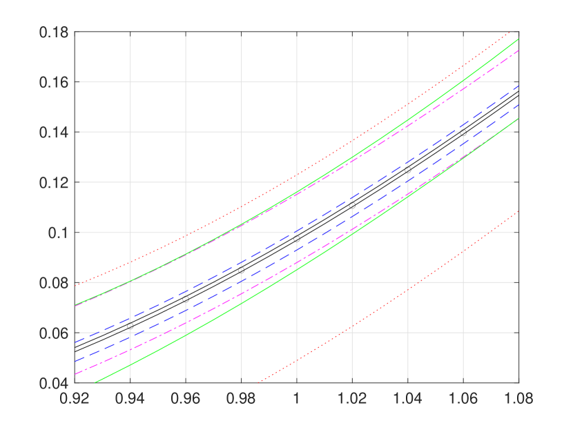
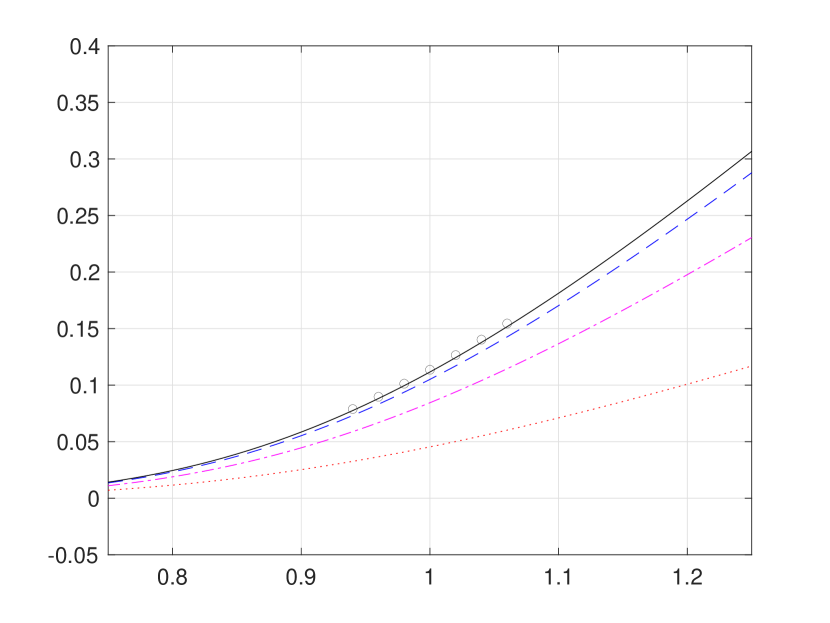
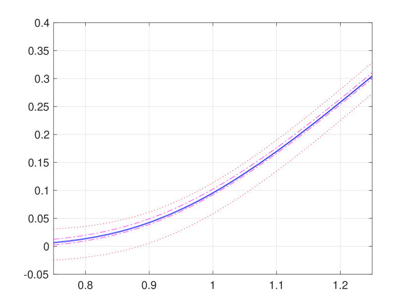
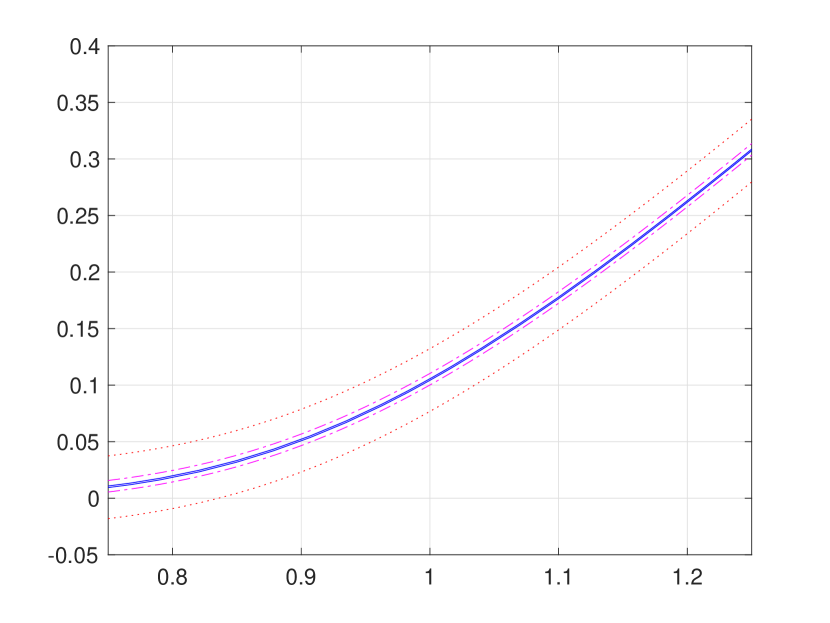
First, we present in Figure 1 iterative weak approximations {wm(0,,i)}m{0,1,2,3}\{w_{m}(0,\cdot,i)\}_{m\in\{0,1,2,3\}}, along with sequences of hard bounding functions {Lm(0,,i;w)}m{0,1,2,3}\{L_{m}(0,\cdot,i;\,w)\}_{m\in\{0,1,2,3\}} and {Um(0,,i;w)}m{0,1,2,3}\{U_{m}(0,\cdot,i;\,w)\}_{m\in\{0,1,2,3\}} for the first three iterations m{0,1,2,3}m\in\{0,1,2,3\}. For a direct comparison with existing numerical results in the literature, we also provide the pointwise approximations reported in [8], as well as the polynomial upper and lower bounds of [4]. Our hard bounding functions converge towards each other quite fast, largely because it is highly likely to observe switching at most three times within the interval [0,T][0,T], indeed with a 98.1%(=Q0,𝐱,i(τ0(4)>T)=(1+1+1/2+1/6)e1)98.1\%(=\mathbb{P}_{Q}^{0,{\bf x},i}(\tau_{0}^{(4)}>T)=(1+1+1/2+1/6)e^{-1}) chance.

Refer to caption
(a) Iterative approximations wm(0,,1)w_{m}(0,\cdot,1)
Refer to caption
(b) Iterative bounds Lm(0,,1;w)L_{m}(0,\cdot,1;\,w) and Um(0,,1;w)U_{m}(0,\cdot,1;\,w)
Refer to caption
(c) Iterative approximations wm(0,,2)w_{m}(0,\cdot,2)
Refer to caption
(d) Iterative bounds Lm(0,,2;w)L_{m}(0,\cdot,2;\,w) and Um(0,,2;w)U_{m}(0,\cdot,2;\,w)
Figure 1: Numerical results for the two-regime setting. Each figure contains m=0m=0 (red dot), m=1m=1 (pink dash-dot), m=2m=2 (blue dash) and m=3m=3 (black solid). The circles provide pointwise approximations as reported in [8], while the green solid lines in (b) and (d) provide the polynomial bounds [4] of degree 10 (green solid).

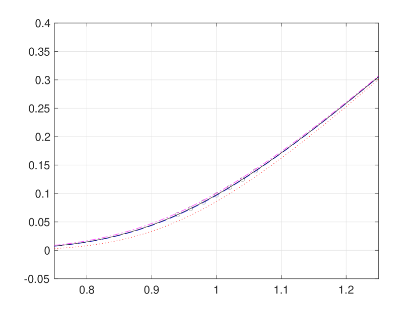
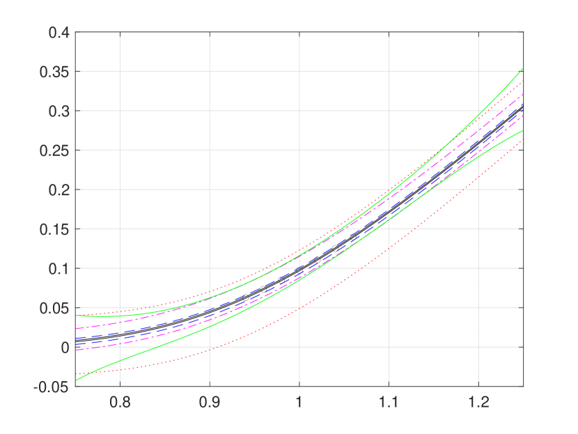
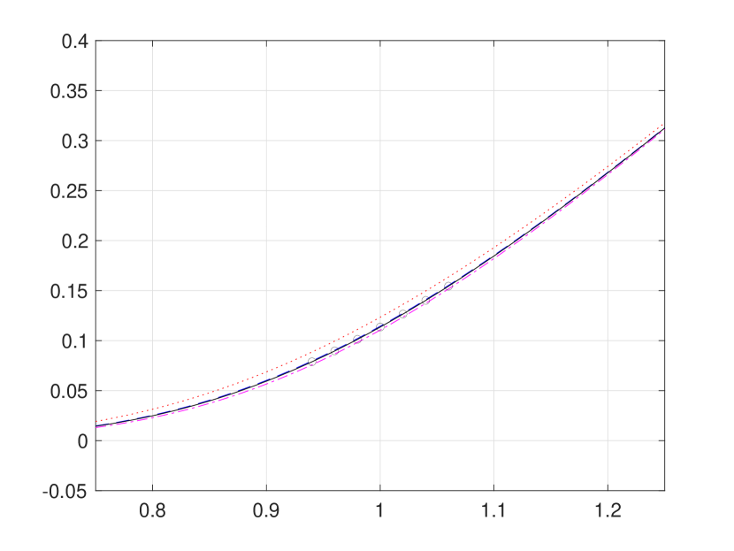
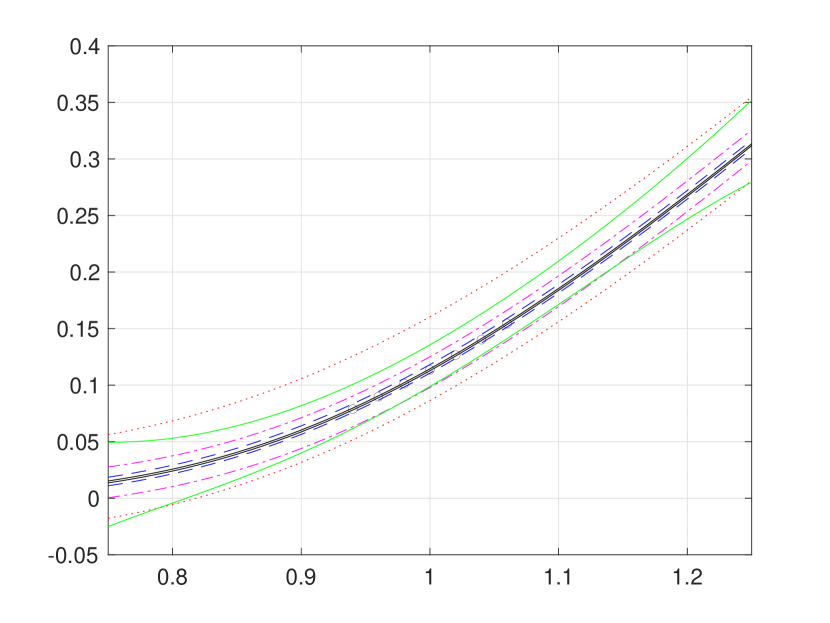
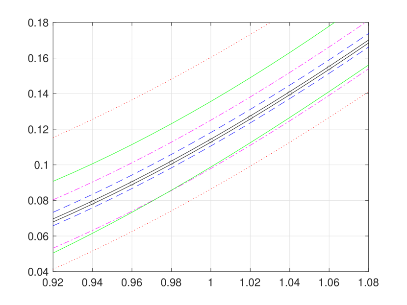
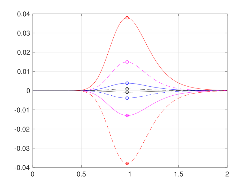
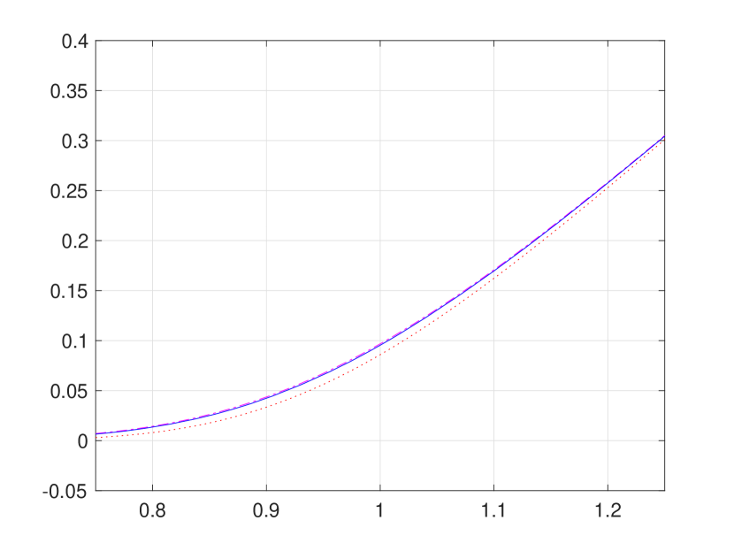
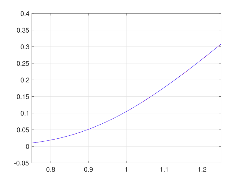
Figure 1 is overly congested with lines and circles to fully illustrate strong agreement of our convergent hard bounding functions {Lm(0,,i;w)}m{0,1,2,3}\{L_{m}(0,\cdot,i;\,w)\}_{m\in\{0,1,2,3\}} and {Um(0,,i;w)}m{0,1,2,3}\{U_{m}(0,\cdot,i;\,w)\}_{m\in\{0,1,2,3\}} with the existing pointwise approximations reported in [8]. Hence, for a better presentation, we provide Figure 2 (a) and (b), respectively, zoom-ins of Figure 1 (b) and (d). In addition, Figure 2 (c) presents the bounds function Nm(0,x,i)N_{m}(0,x,i) defined in (3.24), from which the supremum and infimum {NmL(w)}m{0,1,2,3}\{N_{m}^{L}(w)\}_{m\in\{0,1,2,3\}} and {NmU(w)}m{0,1,2,3}\{N_{m}^{U}(w)\}_{m\in\{0,1,2,3\}} are obtained by numerical approximation, as follows:

(N0L(w),N0U(w),N1L(w),N1U(w),N2L(w),N2U(w),N3L(w),N3U(w))(0.0379,+0.0379,0.0129,+0.0149,0.0039,+0.0039,0.00083,+0.00091).(N_{0}^{L}(w),N_{0}^{U}(w),N_{1}^{L}(w),N_{1}^{U}(w),N_{2}^{L}(w),N_{2}^{U}(w),N_{3}^{L}(w),N_{3}^{U}(w))\\ \approx(-0.0379,+0.0379,-0.0129,+0.0149,-0.0039,+0.0039,-0.00083,+0.00091).
Refer to caption
(a) Zoom-in of Figure 1 (b)
Refer to caption
(b) Zoom-in of Figure 1 (d)
Refer to caption
(c) Bound functions Nm(0,,i;w)N_{m}(0,\cdot,i;w) of (3.24) for m{0,1,2,3}m\in\{0,1,2,3\} and i{1,2}i\in\{1,2\}
Figure 2: Numerical results for the two-regime setting. Figures (a) and (b) zoom in Figure 1 (b) and (d), respectively. Figure (a) provides the bound functions Nm(0,,i)N_{m}(0,\cdot,i) for i=1i=1 (solid) and i=2i=2 (dash), with m=0m=0 (red), m=1m=1 (pink), m=2m=2 (blue) and m=3m=3 (black).

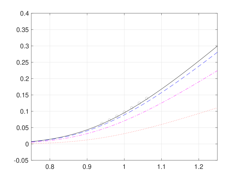
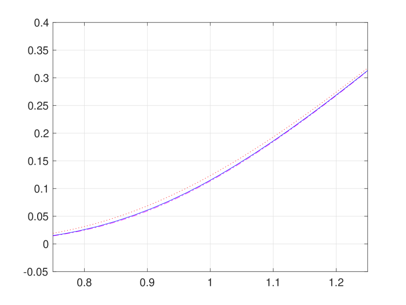
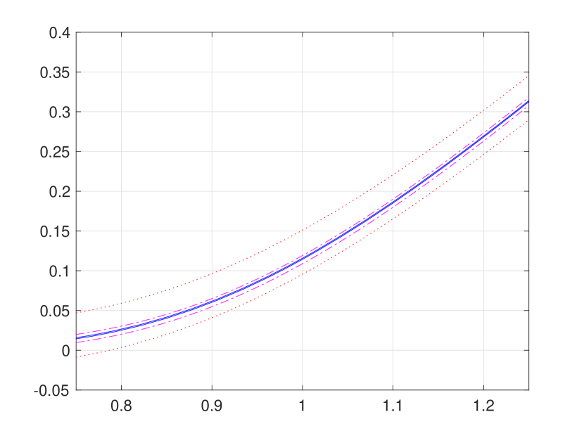
In this problem setting, the initial conditions {g(,i)}i\{g(\cdot,i)\}_{i\in\mathcal{M}} are non-negative and the heat sources {ϕ(,i)}i\{\phi(\cdot,i)\}_{i\in\mathcal{M}} are flat zero. Hence, by Theorem 3.3 (b) and (c), we are here expecting a uniform convergence of the sequence {um(,,i)}m\{u_{m}(\cdot,\cdot,i)\}_{m\in\mathbb{N}} to be also monotonic from below of the target solution vv. In Figure 3, we present the first three iterations, that is, um(t,x,i)u_{m}(t,x,i) for m{0,1,2,3}m\in\{0,1,2,3\}. As expected, the iterative approximations converge monotonically from below (as well as very quickly) towards the pointwise approximations as reported in [8]. We close this section with Figure 4 for numerical results of the sequence {wm}m\{w_{m}\}_{m\in\mathbb{N}} and associated hard bounds {Um(,,;w)}m0\{U_{m}(\cdot,\cdot,\cdot;\,w)\}_{m\in\mathbb{N}_{0}} and {Lm(,,;w)}m0\{L_{m}(\cdot,\cdot,\cdot;\,w)\}_{m\in\mathbb{N}_{0}} for a three-regime case.

Refer to caption
(a) Regime 1: lower bounds um(0,,1)u_{m}(0,\cdot,1)
Refer to caption
(b) Regime 2: lower bounds um(0,,2)u_{m}(0,\cdot,2)
Figure 3: Numerical results for monotonic convergence of {um}m\{u_{m}\}_{m\in\mathbb{N}} in the two-regime setting. Each figure contains m=0m=0 (red dot), m=1m=1 (pink dash-dot), m=2m=2 (blue dash) and m=3m=3 (black solid). The circles provide point-wise approximations as reported in [8].
Refer to caption
(a) Iterative approximations wm(0,,1)w_{m}(0,\cdot,1)
Refer to caption
(b) Iterative approximations wm(0,,2)w_{m}(0,\cdot,2)
Refer to caption
(c) Iterative approximations wm(0,,3)w_{m}(0,\cdot,3)
Refer to caption
(d) Iterative bounds Lm(0,,1)L_{m}(0,\cdot,1) and Um(0,,1)U_{m}(0,\cdot,1)
Refer to caption
(e) Iterative bounds Lm(0,,2)L_{m}(0,\cdot,2) and Um(0,,2)U_{m}(0,\cdot,2)
Refer to caption
(f) Iterative bounds Lm(0,,3)L_{m}(0,\cdot,3) and Um(0,,3)U_{m}(0,\cdot,3)
Figure 4: Numerical results for the three-regime setting with qij=0.5q_{ij}=0.5 for all iji\neq j, r1=r2=r3=0.05r_{1}=r_{2}=r_{3}=0.05, (σ1,σ2,σ3)=(0.15,0.2,0.25)(\sigma_{1},\sigma_{2},\sigma_{3})=(0.15,0.2,0.25), α1=α2=α3=0\alpha_{1}=\alpha_{2}=\alpha_{3}=0, T=1T=1 and K=1.K=1. Each figure contains m=0m=0 (red dot), m=1m=1 (pink dash-dot) and m=2m=2 (blue solid).

6 Concluding remarks

In this paper, we have established a novel convergent iteration framework for a weak approximation of general switching diffusion. By restricting the maximum number of switching, we succeeded to untangle a challenging system of weakly coupled partial differential equations to a collection of independent partial differential equations, for which a variety of accurate and efficient numerical methods are available. Using the sequence of resulting approximate solutions, we constructed upper and lower bounding functions for the unknown solutions. Convergences of the iterative approximate solutions as well as the associated upper and lower bounding functions were rigorously derived and demonstrated through numerical results.

We believe that the developed framework has the potential to be a viable tool for the weak approximation and hard bounding functions for a general class of stochastic differential equations with regime switching. In the present work, in order to fully carry out our theoretical developments and demonstrate all aspects of the developed framework through numerical results, we restricted numerical illustrations to a minimum and did not go into a study of its range of applicability, which is significantly large and should thus be demonstrated in the future. Other future research topics include a investigation of possible issues and cumulative error caused by an iterative use of external numerical techniques, for instance, finite difference methods to approximate wmw_{m} based on the previous approximation for wm1w_{m-1} in the system (3.6), in light of various factors, such as the problem dimension and the input data.

References

  • [1] D. Aingworth, S. Das, and R. Motwani. A simple approach for pricing equity options with Markov switching state variables. Quantitative Finance, 6(2):95–105, 2006.
  • [2] N. A. Baran, G. Yin, and C. Zhu. Feynman-Kac formula for switching diffusions: connections of systems of partial differential equations and stochastic differential equations. Advances in Difference Equations, 2013(1):315, Nov 2013.
  • [3] A. F. Bastani, Z. Ahmadi, and D. Damircheli. A radial basis collocation method for pricing American options under regime-switching jump-diffusion models. Applied Numerical Mathematics, 65:79 – 90, 2013.
  • [4] L. Bhim and R. Kawai. Polynomial upper and lower bounds for financial derivative price functions under regime-switching. Journal of Computational Finance, 22(2):35–71, 2018.
  • [5] N. P. Bollen. Valuing options in regime-switching models. The Journal of Derivatives, 6(1):38–49, 1998.
  • [6] S. Boyarchenko and M. Boyarchenko. Double barrier options in regime-switching hyper-exponential jump-diffusion models. International Journal of Theoretical and Applied Finance, 14(7):1005–1043, 2011.
  • [7] S. Boyarchenko and S. Levendorskiǐ. American options in regime-switching models. SIAM Journal on Control and Optimization, 48(3):1353–1376, 2009.
  • [8] P. Boyle and T. Draviam. Pricing exotic options under regime switching. Insurance: Mathematics and Economics, 40(2):267–282, 2007.
  • [9] R. Elliott, L. Chan, and T. K. Siu. Option pricing and Esscher transform under regime switching. Annals of Finance, 1(4):423–432, 2005.
  • [10] R. Elliott, T. Siu, L. Chan, and J. Lau. Pricing options under a generalized Markov-modulated jump-diffusion model. Stochastic Analysis and Applications, 25(4):821–843, 2007.
  • [11] S. Figlewski and B. Gao. The adaptive mesh model: a new approach to efficient option pricing. Journal of Financial Economics, 53(3):313–351, 1999.
  • [12] A. Friedman. Stochastic Differential Equations and Applications. Academic Press, 1975.
  • [13] P. Hieber and M. Scherer. Efficiently pricing barrier options in a Markov-switching framework. Journal of Computational and Applied Mathematics, 235(3):679–685, 2010.
  • [14] Y. Huang, P. Forsyth, and G. Labahn. Methods for pricing American options under regime switching. SIAM Journal on Scientific Computing, 33(5):2144–2168, 2011.
  • [15] K. Jackson, S. Jaimungal, and V. Surkov. Fourier space time-stepping for option pricing with Lévy models. Journal of Computational Finance, 12(2):1–29, 2008.
  • [16] R. Kawai. Measuring impact of random jumps without sample path generation. SIAM Journal on Scientific Computing, 37(6):A2558–A2582, 2015.
  • [17] A. Q. M. Khaliq, B. Kleefeld, and R. Liu. Solving complex PDE systems for pricing American options with regime-switching by efficient exponential time differencing schemes. Numerical Methods for Partial Differential Equations, 29(1):320–336, 2013.
  • [18] A. Q. M. Khaliq and R. Liu. New numerical scheme for pricing American option with regime-switching. International Journal of Theoretical and Applied Finance, 12(3):319–340, 2009.
  • [19] J. Li, M. Kim, and R. Kwon. A moment approach to bounding exotic options under regime switching. Optimization, 61(10):1–17, 2012.
  • [20] Y. Lu and S. Li. The Markovian regime-switching risk model with a threshold dividend strategy. Insurance: Mathematics and Economics, 44(2):296 – 303, 2009.
  • [21] X. Mao. Stochastic Differential Equations and Their Applications. Woodhead Publishing, 2008.
  • [22] X. Mao and C. Yuan. Stochastic Differential Equations with Markovian Switching. Imperial College Press, London, UK, 2006.
  • [23] M. Perlin. MSRegress - The MATLAB package for Markov regime switching models. SSRN Electronic Journal, April 2015.
  • [24] Q. Qiu and R. Kawai. A decoupling principle for Markov-modulated chains. Statistics & Probability Letters, 182:109301, 2022.
  • [25] Q. Qiu and R. Kawai. A recursive representation for decoupling time-state dependent jumps from jump-diffusion processes. arXiv:2105.13015, 2022.
  • [26] G. Yin, V. Krishnamurthy, and C. Ion. Regime switching stochastic approximation algorithms with application to adaptive discrete stochastic optimization. SIAM Journal on Optimization, 14:1187–1215, 01 2004.
  • [27] G. Yin and C. Zhu. Hybird Switching Diffusions: Properties and Applications. Springer-Verlag New York, 2010.
  • [28] F. L. Yuen and H. Yang. Option pricing with regime switching by trinomial tree method. Journal of Computational and Applied Mathematics, 233(8):1821–1833, 2010.

Appendix A Technical notes

For the sake of completeness, we provide some details of derivation for the computation conducted in the numerical experiments of Sections 5. Since no switching is allowed under 0t,x,i\mathbb{P}_{0}^{t,x,i}, it holds that {Xs:st}\{X_{s}:s\geq t\} satisfies the stochastic differential equation dXs=(riαi)Xsds+σiXsdWsdX_{s}=(r_{i}-\alpha_{i})X_{s}ds+\sigma_{i}X_{s}dW_{s} without switching, that is, under the probability measure 0t,x,i\mathbb{P}_{0}^{t,x,i},

XT=xexp[(riαiσi2/2)(Tt)+σiTtZ],X_{T}\stackrel{{\scriptstyle\mathcal{L}}}{{=}}x\exp\left[(r_{i}-\alpha_{i}-\sigma_{i}^{2}/2)(T-t)+\sigma_{i}\sqrt{T-t}Z\right],

where we reserve ZZ for a general standard normal random variable, independent of the σ\sigma-field \mathcal{F}. Hence, we have

w0(t,x,i)=𝔼0t,x,i[eri(Tt)g(XT)]=𝔼[eri(Tt)g(xexp[(riαiσi2/2)(Tt)+σiTtZ])]=V(x,ri,σi,Tt,αi).w_{0}(t,x,i)=\mathbb{E}_{0}^{t,x,i}\left[e^{-r_{i}(T-t)}g(X_{T})\right]=\mathbb{E}\left[e^{-r_{i}(T-t)}g\left(x\exp\left[(r_{i}-\alpha_{i}-\sigma_{i}^{2}/2)(T-t)+\sigma_{i}\sqrt{T-t}Z\right]\right)\right]=V(x,r_{i},\sigma_{i},T-t,\alpha_{i}).

Since the transition rate qii-q_{ii} is independent of the state variable xx in this problem setting, it follows from (3.14) that

u0(t,x,i)=eqii(Tt)w0(t,x,i)=eqii(Tt)V(x,ri,σi,Tt,αi).u_{0}(t,x,i)=e^{q_{ii}(T-t)}w_{0}(t,x,i)=e^{q_{ii}(T-t)}V(x,r_{i},\sigma_{i},T-t,\alpha_{i}).

We only derive the case m=1m=1, as the further iterations with m{2,}m\in\{2,\cdots\} can be derived along the same line as (3.17) and (3.18). With m=1m=1, it holds by the Fubini theorem that

w1(t,x,i)\displaystyle w_{1}(t,x,i) =u0(t,x,i)+j{i}qijtTeqii(st)𝔼0t,x,i[eri(st)w0(s,Xs,j)]𝑑s\displaystyle=u_{0}(t,x,i)+\sum_{j\in\mathcal{M}\setminus\{i\}}q_{ij}\int_{t}^{T}e^{q_{ii}(s-t)}\mathbb{E}_{0}^{t,x,i}\left[e^{-r_{i}(s-t)}w_{0}(s,X_{s},j)\right]ds
=u0(t,x,i)+j{i}qijtTeqii(st)𝔼0t,x,i[eri(st)𝔼0s,Xs,j[erj(Ts)g(XT)]]𝑑s,\displaystyle=u_{0}(t,x,i)+\sum_{j\in\mathcal{M}\setminus\{i\}}q_{ij}\int_{t}^{T}e^{q_{ii}(s-t)}\mathbb{E}_{0}^{t,x,i}\left[e^{-r_{i}(s-t)}\mathbb{E}_{0}^{s,X_{s},j}\left[e^{-r_{j}(T-s)}g(X_{T})\right]\right]ds,

due to the non-negativity of the integrands. Next, for each s[0,T]s\in[0,T], we have

𝔼0s,Xs,j[erj(Ts)g(XT)]=𝔼[erj(Ts)g(Xsexp[(rjαjσj2/2)(Ts)+σj(WTWs)])|s],\mathbb{E}_{0}^{s,X_{s},j}\left[e^{-r_{j}(T-s)}g(X_{T})\right]=\mathbb{E}\left[e^{-r_{j}(T-s)}g\left(X_{s}\exp\left[(r_{j}-\alpha_{j}-\sigma_{j}^{2}/2)(T-s)+\sigma_{j}(W_{T}-W_{s})\right]\right)\Big{|}\,\mathcal{F}_{s}\right],

which yields

𝔼0t,x,i[eri(st)𝔼0s,Xs,j[erj(Ts)g(XT)]]\displaystyle\mathbb{E}_{0}^{t,x,i}\left[e^{-r_{i}(s-t)}\mathbb{E}_{0}^{s,X_{s},j}\left[e^{-r_{j}(T-s)}g(X_{T})\right]\right]
=𝔼0t,x,i[eri(st)𝔼[erj(Ts)g(Xsexp[(rjαjσj2/2)(Ts)+σj(WTWs)])|s]]\displaystyle\quad=\mathbb{E}_{0}^{t,x,i}\left[e^{-r_{i}(s-t)}\mathbb{E}\left[e^{-r_{j}(T-s)}g\left(X_{s}\exp\left[(r_{j}-\alpha_{j}-\sigma_{j}^{2}/2)(T-s)+\sigma_{j}(W_{T}-W_{s})\right]\right)\Big{|}\mathcal{F}_{s}\right]\right]
=𝔼[eri(st)𝔼[erj(Ts)g(xexp[(riαiσi2/2)(st)+σi(WsWt)]exp[(rjαjσj2/2)(Ts)+σj(WTWs)])|s]]\displaystyle\quad=\mathbb{E}\left[e^{-r_{i}(s-t)}\mathbb{E}\left[e^{-r_{j}(T-s)}g\left(x\exp\left[(r_{i}-\alpha_{i}-\sigma_{i}^{2}/2)(s-t)+\sigma_{i}(W_{s}-W_{t})\right]\exp\left[(r_{j}-\alpha_{j}-\sigma_{j}^{2}/2)(T-s)+\sigma_{j}(W_{T}-W_{s})\right]\right)\Big{|}\mathcal{F}_{s}\right]\right]
=𝔼[er(s)(Tt)g(xexp[(r(s)α(s)σ2(s)/2)(Tt)+σ(s)TtZ])]=V(x,r(s),σ(s),Tt,α(s)),\displaystyle\quad=\mathbb{E}\left[e^{-r(s)(T-t)}g\left(x\exp\left[(r(s)-\alpha(s)-\sigma^{2}(s)/2)(T-t)+\sigma(s)\sqrt{T-t}Z\right]\right)\right]=V(x,r(s),\sigma(s),T-t,\alpha(s)),

where the third equality holds because the sum of two independent centered normal random variables with variances σi2(st)\sigma^{2}_{i}(s-t) and σj2(Ts)\sigma^{2}_{j}(T-s) is identical in law to a centered normal random variable variance σi2(st)+σj2(Ts)=σ2(s)(Tt)\sigma^{2}_{i}(s-t)+\sigma^{2}_{j}(T-s)=\sigma^{2}(s)(T-t). Note that the expectation from the third line on can be understood to be with respect to the underlying Brownian motion alone. Therefore, we obtain

w1(t,x,i)\displaystyle w_{1}(t,x,i) =u0(t,x,i)+j{i}qijtTeqii(st)V(x,r(s),σ(s),Tt,α(s))𝑑s,\displaystyle=u_{0}(t,x,i)+\sum_{j\in\mathcal{M}\setminus\{i\}}q_{ij}\int_{t}^{T}e^{q_{ii}(s-t)}V(x,r(s),\sigma(s),T-t,\alpha(s))ds,
u1(t,x,i)\displaystyle u_{1}(t,x,i) =u0(t,x,i)+j{i}qijtTeqii(st)+qjj(Ts)V(x,r(s),σ(s),Tt,α(s))𝑑s.\displaystyle=u_{0}(t,x,i)+\sum_{j\in\mathcal{M}\setminus\{i\}}q_{ij}\int_{t}^{T}e^{q_{ii}(s-t)+q_{jj}(T-s)}V(x,r(s),\sigma(s),T-t,\alpha(s))ds.

The second and further iterations can be derived in a similar manner.