ITSO: A novel Inverse Transform Sampling-based Optimization algorithm for stochastic search
Abstract
Optimization algorithms appear in the core calculations of numerous Artificial Intelligence (AI) and Machine Learning methods, as well as Engineering and Business applications. Following recent works on the theoretical deficiencies of AI, a rigor context for the optimization problem of a black-box objective function is developed. The algorithm stems directly from the theory of probability, instead of a presumed inspiration, thus the convergence properties of the proposed methodology are inherently stable. In particular, the proposed optimizer utilizes an algorithmic implementation of the -dimensional inverse transform sampling as a search strategy. No control parameters are required to be tuned, and the trade-off among exploration and exploitation is by definition satisfied. A theoretical proof is provided, concluding that only falling into the proposed framework, either directly or incidentally, any optimization algorithm converges in the fastest possible time. The numerical experiments, verify the theoretical results on the efficacy of the algorithm apropos reaching the optimum, as fast as possible.
Keywords: Stochastic Optimization, Inverse Transform Sampling, Black-box Function, Global Convergence.
1 Introduction
Despite the numerous research works and industrial applications of Artificial Intelligence algorithms, they have been criticized about lacking a solid theoretical background [1]. The empirical results demonstrate impressive performance, however, their theoretical foundation and analysis are often vague [2]. Machine Learning (ML) models, frequently aim at identifying an optimal solution [3, 4], which is computationally hard and attempts to explain the procedure often based on the evaluation of the function’s Gradients [5, 6]. Accordingly, the identification of whether a stochastic algorithm will work or not remains an open question for many research and real-world applications [7, 8, 9, 10]. A vast number of optimization algorithms have been developed and applied for the solution of the corresponding problems [11, 12, 13, 14], as well as mathematical proofs regarding their algorithmic convergence [15, 16, 17], however, their basic formulation often stems from nature-inspired procedures [18, 19] and not solid mathematical frameworks. Accordingly, a vast number of research works have been published in order to investigate the performance of black-box algorithms [20, 21, 22].
In its elementary form, the purpose of efficient optimization algorithms is to find the argument yielding the minimum value of a black-box function , defined on a set , . Accordingly, the inverse problem of maximization is the minimization of the negated function , while problems with multiple objective functions often utilize single function optimization algorithms to attain the best possible solution. is assumed a compact subset of the Euclidean space , where is the number of dimensions of the set , however, the proposed method applies similarly to discrete and continuous topological spaces. The unknown, black-box function , returns values for the given input at each computational discrete time step , where is the number of maximum function evaluations. The sought solution is a vector , such that , which may be written by
| (1) |
The purpose of this work is to provide a rigor context for the optimization problem of a black-box function, by adhering to the Probability Theory, aiming at identifying the best possible solution , within the given iterations , during the execution of the algorithm.
The rest of the paper is organized as follows: In Section 2, the proposed Inverse Transform Sampling Optimizer (ITSO) is presented. Additionally, the same Section provides in details the theoretical formulation of the algorithm as well as some programming and implementation techniques. Illustrative examples of the optimization history are also comprised. In Section 3 the theoretical proof of convergence is provided, as well as Lemma 1, deriving that the suggested optimization framework is the fastest possible. The numerical experiments are divided into three groups. Subsection 5 is about the comparison with 13 nonlinear loss functions, 17 optimization methods, for 10 and 20 dimensions of search space, and 5000 and 10000 iterations per dimension. Section 4, briefly presents the programming techniques that were investigated, in order to implement the proposed method into a computer code. Finally, the conclusions are drawn in Section 6.
2 Optimization by Inverse Transform Sampling
Let the probability distribution of the optimal values of , be considered as the product of some monotonically decreasing kernel over at some time-step and hence given input . This assumption stands in the foundation of the method and can be considered as rational, instead of an arbitrary selection strategy, inspired by natural or other phenomena. It is a straightforward application of the Probability theory to the problem. The kernel may be considered as parametric, concerning time . The selection of the kernel should satisfy the condition that its limit is the Dirac delta function centered at ,
| (2) |
where denotes the Dirac function centered at . Although the selection of the kernel is ambiguous, it can be chosen among a variety of functions satisfying Equation 2, such as the Gaussian:
| (3) |
where is a time increasing pattern. The function controls the shape of the kernel , approximating numerically Equation 2. Additionally, we may use:
| (4) |
| (5) |
or any other non-negative Lebesgue-integrable function, which reverses the order of the given set of all , where is the permutation of the indices , such that the sequence of being monotonically strictly decreasing. The duplicate values of should be extracted to avoid numerical instabilities. These duplicates often appeared in the empirical calculations, especially when the algorithm was close to a local or global stationary point. A variety of kernel functions were investigated, and the results weren’t affected significantly, even when distorting with some random noise .
Accordingly, for each dimension of the vector space , the marginal probability density function is obtained numerically from the kernel function:
| (6) |
is the probability that falls within the infinitesimal interval . The corresponding cumulative distribution function (CDF) , can be calculated by:
| (7) |
where is the lower bound of the dimension of the vector space and can be numerically evaluated by some numerical integration rule, such as the Riemann sum , with computed by the application of the kernel on some , such that , or another approximation scheme. In the following pseudo-code 1, the algorithmic implementation of the Inverse Transform Sampling method is demonstrated. The symbols are also noted in the Nomenclature section.
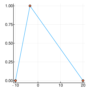
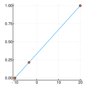
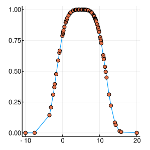
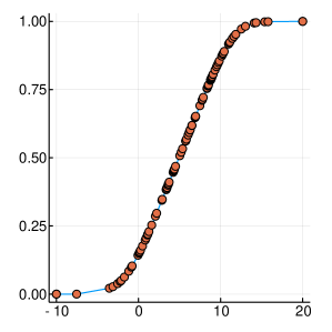
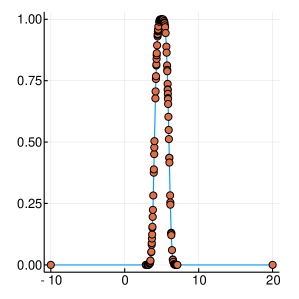
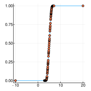
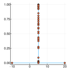
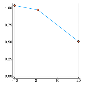
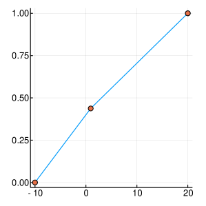
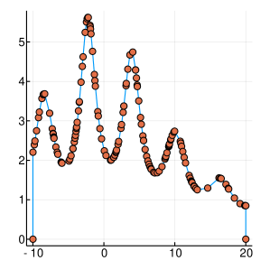
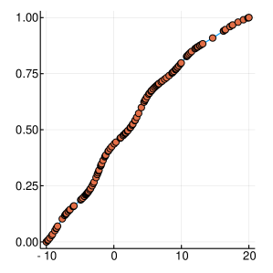
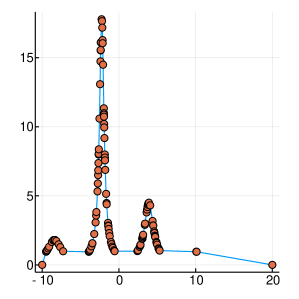
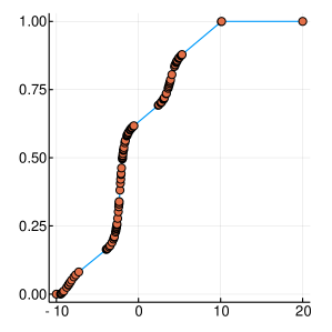
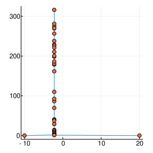
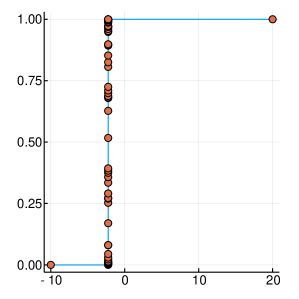
A graphical demonstration of the evolution of the Probability Density, as well as the corresponding Cumulative Distribution Functions, is presented in Figure 1, for , which is function with one extreme value and in Figure 2, for , which has many extrema. Interestingly, as the function evaluations increase, the CDF, is characterised by sharp slopes, which are positioned in regions where the PDF exhibits high values, and hence function attends its lows. Figures 1 and 2, offer an intuitive representation of the procedure for finding the minimum of the function, within the suggested framework.

3 Convergence Properties
During the optimization process, the algorithm generates some input variables as arguments for the black-box function . By utilizing the values of , we may compute the values of the distribution , by Equation 6, and by Equation 7, for all .
Definition 1.
We define the argument of within iterations, corresponding to the minimum of as .
In iteration , the algorithm will have searched the space , within the limits . By definition, is the probability density (likelihood) that the optimum occurs in a region . Hence,
| (8) |
where , denotes the expectation of a random variable or vector.
Theorem 1.
If tends to Dirac , then ITSO will converge to
Proof.
For each dimension , we may write
| (9) |
and integrating by parts, we obtain
| (10) |
If we apply the theorem of the antiderivative of inverse functions [23], we obtain
| (11) |
With subscript denoting that the Dirac function is centered at the argument that minimizes , i.e.
| (13) |
and
| (14) |
As tends to Dirac function, tends to the Heaviside step function centered at , hence by Equation 12 we deduce that
| (15) |
Lemma 1.
(ITSO Convergence Speed) ITSO is the fastest possible optimization framework
Proof.
Any distribution that doesn’t tend to Dirac, could be considered as a Dirac plus a positive function of . In this case, the algorithmic framework would search through a strategy that produces a over , as
| (17) |
| (18) |
.
Hence the algorithm would converge to a point different than
∎
4 Programming techniques
A variety of programming techniques were investigated, in order to implement the proposed method into a computer code. To keep the algorithm simple and reduce the computational time, we applied inverse transform sampling by keeping in each iteration the best function evaluations, and randomly sampling among them. This is equivalent to a kernel function that vanishes over the worst function evaluations, and distributing the probability mass to the best performing ones. Accordingly, similar programming techniques may be investigated in future works, within the suggested framework.
The Algorithm 2 represents a simple version of the supplementary code in the appendix, which may easily be programmed. The variable is a dynamic vector, containing all values of the objective function returned during the optimization history, until step , and is an matrix, containing all the design vectors , corresponding to . The integer is a parameter regarding how many instances of the optimization history are kept in order to randomly sample among them; for example if , we may select . In this variation of the code, the Inverse Transform Sampling is approximately implemented in line 7, by calculating the random variable , among the extrema of the vector , corresponding to the range where: for the dimension of all , the best function values were returned by the black-box function . The sought solution is the vector , and the mimimum attained value of the objective function .
5 Numerical Experiments
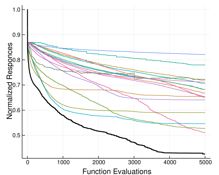
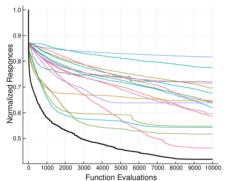
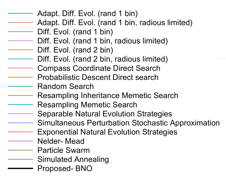
In this section, we present the results obtained by running the ITSO algorithm, as well as Adaptive Differential Evolution (rand 1 bin), Differential Evolution (rand 1 bin), and Differential Evolution (rand 2 bin) with and without radius limited, Compass Coordinate Direct Search, Probabilistic Descent Direct search, Random Search, Resampling Inheritance Memetic Search, Resampling Memetic Search, Separable Natural Evolution Strategies, Simultaneous Perturbation Stochastic Approximation, and Exponential Natural Evolution Strategies from the Julia Package BlackBoxOptim.jl [24], and Nelder-Mead, Particle Swarm, and Simulated Annealing from Optim.jl [25]. To demonstrate the performance of each optimizer in attaining the minimum, we firstly run the algorithm times, obtain for and all iterations , and average the results
| (20) |
Then, we normalize the vector of obtained function evaluations in the domain through
| (21) |
and finally use the optimization history
| (22) |
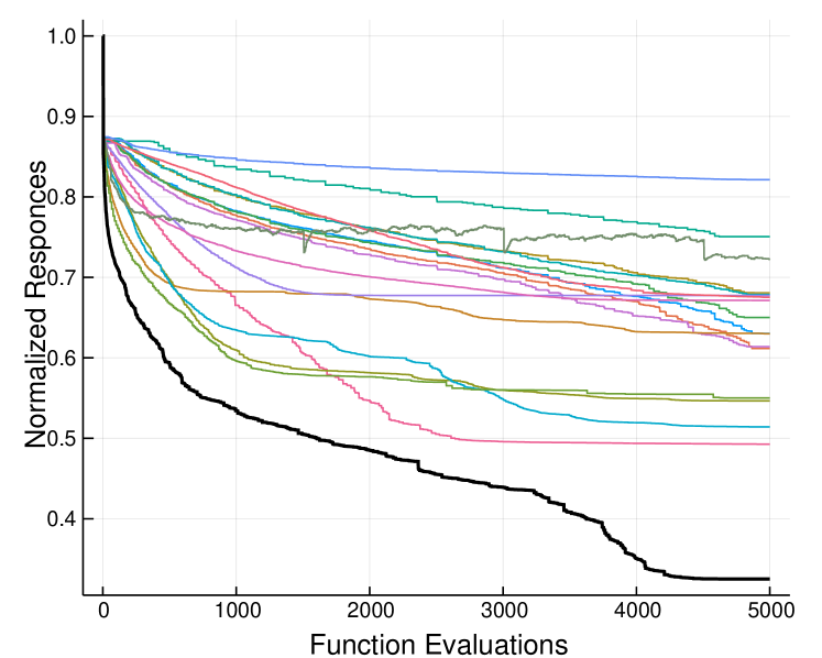
where indicates the number of black-box functions used for the evaluation. Equation 22 was selected as a performance metric, in order to obtain a clear representation of the various optimizers utilized, as powers smaller than one (in our case ), have the property to magnify the attained values at the final steps of the optimization history. In Figure 3 the numerical experiments for functions are presented. Each line corresponds to the normalized average optimization history (Equation 22, for all functions, which were repeated 10 times). We may see a clear prevalence of the proposed framework, in terms of convergence performance, as expected by the theoretical investigation. The numerical experiments for the comparison with other optimizers, may be reproduced by running the file __run.jl.
|
0.00991 | 0.02210 | 0.00852 | |
|
0.00734 | 0.01762 | 0.00482 | |
|
0.01348 | 0.02196 | 0.01161 | |
|
0.00760 | 0.01377 | 0.00564 | |
|
0.02140 | 0.03712 | 0.02687 | |
|
0.02072 | 0.03110 | 0.02008 | |
|
0.00084 | 0.00118 | 0.00045 | |
|
0.00984 | 0.01424 | 0.01239 | |
| Random Search | 0.05678 | 0.08307 | 0.07936 | |
|
0.00238 | 0.00513 | 0.00243 | |
|
0.00129 | 0.00236 | 0.00223 | |
|
0.02038 | 0.01165 | 0.01127 | |
|
0.13967 | 0.13998 | 0.13227 | |
|
0.01972 | 0.01415 | 0.01286 | |
| Nelder-Mead | 0.01858 | 0.03307 | 0.03452 | |
| Particle Swarm | 0.00254 | 0.00166 | 0.00136 | |
|
0.03825 | 0.03812 | 0.03721 | |
| Proposed-ITSO | 0.00001 | 0.00020 | 0.00017 |
6 Discussion and Conclusions
In this work a novel approach was presented for the well known problem of finding the argument that minimizes a black-box, function or system. A vast volume of approximation algorithms have been proposed, mainly heuristic, such as genetic, evolutionary, particle swarm, as well as their variations. However, they stem from nature-inspired procedures, and hence their converge is investigated a-posteriori. Despite their efficiency, they are often deprecated by researchers, due to the lack of rigorous mathematical formulation, as well as complexity of implementation. To the contrary, the proposed algorithm, initiates its formulation from well established probabilistic definitions and theorems, and its implementation demands a few lines of computer code. Furthermore, the convergence properties were found stable, as a proof that the suggested framework attains the best possible solution in the fewest possible iterations. The numerical examples validate the theoretical results and may be reproduced by the provided computer code. We consider the suggested method as a powerful framework which may easily be adopted to the sought solution of any problem involving the minimization of a black-box function.
Appendix A Programming Code
The corresponding computer code is available on GitHub https://github.com/nbakas/ITSO.jl. The examples of Figure 3 may be reproduced by running __run.jl. The sort version of the Algorithm 1 is available in Julia [26] (file ITSO-short.jl), Octave [27] (ITSOshort.m), and Python [28] (ITSO-short.py). The implementation of the framework is integrated in a few lines of computer code, which can be easily adapted for case specific applications with high efficiency.
Appendix B Black-Box Functions
The following functions were used for the numerical experiments. Equations 23, 24 (Elliptic, Cigar), were utilized from [29], Cigtab (Eq. 25), Griewank 26 from [30], Quartic (Eq. 27 from [31], Schwefel (Eq. 28), Rastrigin (Eq. 29), Sphere (Eq. 30), and Ellipsoid (Eq. 31) from [32, 24], and Alpine (Eq. 32) from [33]. Equations 33, 34, 35, were developed by the authors. The code implementation for the selected equations appears in file functions_opti.jl in the supplementary computer code.
The exact variation used in this work is as follows, where we have adopted the notation presented in the Nomenclature section, where denotes the step of the optimization history, and the dimension of the design variable .
| (23) | |||
| (24) |
| (25) |
| (26) |
| (27) |
| (28) | |||
| (29) | |||
| (30) |
| (31) |
| (32) |
| (33) |
| (34) |
| (35) |
References
- [1] M. Hutson, “AI researchers allege that machine learning is alchemy,” Science, may 2018. [Online]. Available: http://www.sciencemag.org/news/2018/05/ai-researchers-allege-machine-learning-alchemy
- [2] D. Sculley, J. Snoek, A. Rahimi, and A. Wiltschko, “Winner’s Curse? On Pace, Progress, and Empirical Rigor,” ICLR Workshop track, 2018.
- [3] S. Sra, S. Nowozin, and S. J. Wright, Optimization for machine learning. Mit Press, 2012.
- [4] L. Bottou, F. E. Curtis, and J. Nocedal, “Optimization methods for large-scale machine learning,” Siam Review, vol. 60, no. 2, pp. 223–311, 2018.
- [5] C. Rudin, “Stop explaining black box machine learning models for high stakes decisions and use interpretable models instead,” Nature Machine Intelligence, vol. 1, no. 5, pp. 206–215, 2019. [Online]. Available: https://doi.org/10.1038/s42256-019-0048-x
- [6] J. Wu, M. Poloczek, A. G. Wilson, and P. Frazier, “Bayesian optimization with gradients,” in Advances in Neural Information Processing Systems, 2017, pp. 5267–5278.
- [7] B. Doerr, “Probabilistic tools for the analysis of randomized optimization heuristics,” in Theory of Evolutionary Computation. Springer, 2020, pp. 1–87.
- [8] C. Doerr, “Complexity theory for discrete black-box optimization heuristics,” in Theory of Evolutionary Computation. Springer, 2020, pp. 133–212.
- [9] M. Papadrakakis, N. D. Lagaros, and V. Plevris, “Design optimization of steel structures considering uncertainties,” Engineering Structures, vol. 27, no. 9, pp. 1408–1418, 2005.
- [10] ——, “Optimum design of space frames under seismic loading,” International Journal of Structural Stability and Dynamics, vol. 1, no. 01, pp. 105–123, 2001.
- [11] N. Moayyeri, S. Gharehbaghi, and V. Plevris, “Cost-based optimum design of reinforced concrete retaining walls considering different methods of bearing capacity computation,” Mathematics, vol. 7, no. 12, p. 1232, 2019.
- [12] V. Plevris and M. Papadrakakis, “A hybrid particle swarm—gradient algorithm for global structural optimization,” Computer-Aided Civil and Infrastructure Engineering, vol. 26, no. 1, pp. 48–68, 2011.
- [13] N. D. Lagaros, N. Bakas, and M. Papadrakakis, “Optimum Design Approaches for Improving the Seismic Performance of 3D RC Buildings,” Journal of Earthquake Engineering, vol. 13, no. 3, pp. 345–363, mar 2009. [Online]. Available: http://www.tandfonline.com/doi/full/10.1080/13632460802598594
- [14] N. D. Lagaros, M. Papadrakakis, and N. P. Bakas, “Automatic minimization of the rigidity eccentricity of 3D reinforced concrete buildings,” Journal of Earthquake Engineering, vol. 10, no. 4, pp. 533–564, jul 2006. [Online]. Available: http://www.tandfonline.com/doi/full/10.1080/13632460609350609
- [15] A. D. Bull, “Convergence rates of efficient global optimization algorithms,” Journal of Machine Learning Research, vol. 12, no. Oct, pp. 2879–2904, 2011.
- [16] G. Rudolph, “Convergence analysis of canonical genetic algorithms,” IEEE transactions on neural networks, vol. 5, no. 1, pp. 96–101, 1994.
- [17] M. Clerc and J. Kennedy, “The particle swarm-explosion, stability, and convergence in a multidimensional complex space,” IEEE transactions on Evolutionary Computation, vol. 6, no. 1, pp. 58–73, 2002.
- [18] K. R. Opara and J. Arabas, “Differential evolution: A survey of theoretical analyses,” Swarm and evolutionary computation, vol. 44, pp. 546–558, 2019.
- [19] N. Razmjooy, V. V. Estrela, H. J. Loschi, and W. Fanfan, “A comprehensive survey of new meta-heuristic algorithms,” Recent Advances in Hybrid Metaheuristics for Data Clustering, Wiley Publishing, 2019.
- [20] M. A. Muñoz and K. A. Smith-Miles, “Performance analysis of continuous black-box optimization algorithms via footprints in instance space,” Evolutionary computation, vol. 25, no. 4, pp. 529–554, 2017.
- [21] C. Audet and W. Hare, Derivative-free and blackbox optimization. Springer, 2017.
- [22] C. Audet and M. Kokkolaras, “Blackbox and derivative-free optimization: theory, algorithms and applications,” 2016.
- [23] F. D. Parker, “Integrals of Inverse Functions,” The American Mathematical Monthly, vol. 62, no. 6, p. 439, jun 1955. [Online]. Available: http://www.jstor.org/stable/2307006?origin=crossref
- [24] R. Feldt, “Blackboxoptim.jl,” 2013-2018. [Online]. Available: https://github.com/robertfeldt/BlackBoxOptim.jl
- [25] J. Myles White, T. Holy, O. Contributors (2012), P. Kofod Mogensen, J. Myles White, T. Holy, P. Contributors (2016), Other. Kofod Mogensen, A. Nilsen Riseth, J. Myles White, T. Holy, and O. Contributors (2017), “Optim.jl,” 2012,2016,2017. [Online]. Available: https://github.com/JuliaNLSolvers/Optim.jl
- [26] J. Bezanson, A. Edelman, S. Karpinski, and V. B. Shah, “Julia: A fresh approach to numerical computing,” SIAM review, vol. 59, no. 1, pp. 65–98, 2017.
- [27] Contributors, “Gnu octave,” http://hg.savannah.gnu.org/hgweb/octave/file/tip/doc/interpreter/contributors.in, 28 Feb 2020.
- [28] ——, “Python 3.8.2,” https://www.python.org/, 2020.
- [29] J. Liang, B. Qu, P. Suganthan, and A. G. Hernández-Díaz, “Problem definitions and evaluation criteria for the cec 2013 special session on real-parameter optimization,” Computational Intelligence Laboratory, Zhengzhou University, Zhengzhou, China and Nanyang Technological University, Singapore, Technical Report, vol. 201212, no. 34, pp. 281–295, 2013.
- [30] C.-K. Au and H.-F. Leung, “Eigenspace sampling in the mirrored variant of (1, )-cma-es,” in 2012 IEEE Congress on Evolutionary Computation. IEEE, 2012, pp. 1–8.
- [31] M. Jamil and X.-S. Yang, “A literature survey of benchmark functions for global optimization problems,” arXiv preprint arXiv:1308.4008, 2013.
- [32] S. Finck, N. Hansen, R. Ros, and A. Auger, “Real-parameter black-box optimization benchmarking 2009: Presentation of the noiseless functions,” Citeseer, Tech. Rep., 2010.
- [33] K. Hussain, M. N. M. Salleh, S. Cheng, and R. Naseem, “Common benchmark functions for metaheuristic evaluation: A review,” JOIV: International Journal on Informatics Visualization, vol. 1, no. 4-2, pp. 218–223, 2017.