Jarzynski equality and the second law of thermodynamics beyond the weak-coupling limit: The quantum Brownian oscillator
Abstract
We consider a time-dependent quantum linear oscillator coupled to a bath at an arbitrary strength. We then introduce a generalized Jarzynski equality (GJE) which includes the terms reflecting the system-bath coupling. This enables us to study systematically the coupling effect on the linear oscillator in a non-equilibrium process. This is also associated with the second law of thermodynamics beyond the weak-coupling limit. We next take into consideration the GJE in the classical limit. By this generalization we show that the Jarzynski equality in its original form can be associated with the second law, in both quantal and classical domains, only in the vanishingly small coupling regime.
pacs:
05.40.JcBrownian motion and 05.70.-aThermodynamics1 Introduction
Since it was introduced, the Jarzynski equality (JE) has been attracting a great deal of interest due to its remarkable attribute. It explicitly states that if a given system, initially prepared in thermal equilibrium, is driven far from this equilibrium by an external perturbation, then this non-equilibrium process satisfies JAR97
| (1) |
where the symbol denotes the microscopic work performed on the system in a single run for a variation of the external parameter according to the pre-determined protocol, and the symbol is the probability distribution of the work value ; the symbol denotes the inverse temperature of the environment, and is the Helmholtz free energy change of the system between the initial and final states, equivalent to the average reversible work in the corresponding isothermal process CAL85 . As such, the average is evaluated over a large number of runs. Then, applying the Jensen inequality to the JE (1), we can easily obtain as an expression of the second law of the thermodynamics JAR08 ; BOK10 . Further, as a generalization of JE, Crooks introduced the fluctuation theorem given by CRO98 ; CRO99
| (2) |
where the symbols and are the probability densities of performing the work when its protocol runs in the forward and reverse directions, respectively.
The JE has been verified in experiments with small-scale systems, where the fluctuations of work values are sufficiently observable JAR02 , e.g., in determination of the free energy change between the unfolded and folded conformations of a single RNA molecule LIP02 ; BUS05 . However, its strict validity is still in dispute, especially in association with the second law beyond the weak coupling between system and bath (see, e.g., an instructive critique in COH04 as well as Jarzynski’s reply in JAR04 ).
The JE has also been discussed in the quantum domain, where no notion of trajectory in the phase space is available and so instead the spectrum information has to be used for determination of the work probability distribution . Most of those attempts were made within isolated or weakly-coupled systems TAS00 ; MUK03 ; ROE04 ; ESP06 ; TAL07 ; MAH07 ; ENG07 ; CRO08 ; AND08 ; DEF08 ; TAK09 ; MAH10 ; MAH11 ; NGO12 . However, the finite coupling strength between system and bath in small-scale devices gives rise to some quantum subtleties which can no longer be neglected for studying the thermodynamic properties of such devices SHE02 ; MAH04 ; CAP05 .
In CAM09 , the fluctuation theorem (2), immediately reproducing the JE, was discussed for arbitrary open quantum systems with no restriction on the coupling strength. Its key idea was such that if the total system (i.e., open quantum system plus bath) is initially in a thermal canonical state, but otherwise isolated, and an external perturbation acts solely on the open system, then the work performed on the total system may be interpreted as the work performed on the open system alone. Then the final result was explicitly obtained [cf. (17)-(17a)] by mimicking the classical case such that the work on the system-of-interest beyond the weak-coupling limit is directly related to the free energy change of a potential of mean force JAR04
where the symbols and denote the bath and interaction Hamiltonians, respectively; note here that on the right-hand side the -dependency exists only in [cf. (16)]. This quantum result was subsequently applied to a solvable model (e.g., TAL09 ).
However, as will be discussed below, it is not clear if this quantum fluctuation theorem is associated directly with the system-of-interest alone, beyond the weak-coupling limit, being the quantum description of in (1); in fact, an attempt to relate the quantum description of to the second law of thermodynamics within the coupled system would even lead to a violation of this law. In this paper we intend to resolve this issue, within a time-dependent quantum Brownian oscillator as a mathematically manageable scheme, by introducing explicitly a generalized Jarzynski equality (GJE) directly associated with the open system with no restriction on the coupling strength, and then discussing the resultant second law with no violation. The general layout of this paper is the following. In Sect. 2 we briefly review the results known from the references and useful for our discussions. In Sect. 3 we discuss the second law beyond the weak-coupling regime, which shows that the JE in its known form can be associated with this law only in the vanishingly small coupling regime. In Sect. 4 we introduce the GJE consistent with the second law, valid at an arbitrary coupling strength. Finally we give the concluding remarks of this paper in Sect. 5.
2 Quantum Brownian oscillator in a non-equilibrium thermal process
The quantum Brownian oscillator in consideration is given by the Caldeira-Leggett model Hamiltonian ING98 ; WEI08
| (4) |
where a system linear oscillator, a bath, and a system-bath interaction are given by
| (4a) | ||||
| (4b) | ||||
| (4c) |
respectively. Here the angular frequency varies in the time interval according to an arbitrary but pre-determined protocol (for the sake of convenience, let in what follows), and the constants denote the coupling strengths. The total system initially prepared is in a canonical thermal equilibrium state with the initial partition function . Then the initial internal energy of the coupled oscillator is given by , where the initial state of the oscillator . Here the symbol denotes the partial trace for the bath degrees of freedom only; it is explicitly given by GRA88 ; WEI08
expressed in terms of the equilibrium fluctuations, and . Beyond the weak-coupling limit, this reduced density matrix is not any longer in form of a canonical thermal state , immediately leading to the fact that the coupled oscillator is not with its well-defined local equilibrium temperature KIM10 .
For the below discussions, we will need the fluctuation-dissipation theorem in the initial (equilibrium) state FOR88
Here the dynamic susceptibility is given by
| (7) |
where the symbol denotes the Fourier-Laplace transformed damping kernel. This can be rewritten as LEV88
| (7a) |
in terms of the normal-mode frequencies of the total system . It is straightforward to verify that for an uncoupled (or isolated) oscillator (i.e., all system-bath coupling strengths ).
From (2), it follows that FOR85
| (8a) | |||||
| (8b) | |||||
as well-known, both of which give the initial internal energy of the coupled oscillator
| (9) | |||
In the absence of the system-bath coupling, this reduces to the well-known expression of internal energy CAL85
| (9a) |
where the average quantum number . With , its classical value also appears as .
In comparison, there is a widely used alternative approach to the thermodynamic energy of the coupled oscillator in equilibrium, given by FOR05 ; HAE05 ; HAE06 ; FOR06 ; KIM06 ; KIM07 ; the symbol denotes the reduced partition function associated with the Hamiltonian of mean force CAM09 ; JAR04
| (10) |
and thus with the partition function associated with the isolated bath . With the vanishing coupling strengths (), this partition function precisely reduces, as required, to its standard form of for an isolated oscillator. Then it can be shown that HAE06
| (11a) | |||
| with and , whereas | |||
| (11b) | |||
It is seen that unless the damping model is Ohmic. In fact, all thermodynamic quantities resulting from the partition function cannot exactly describe the well-defined thermodynamics of the reduced system in its state (2) beyond the weak-coupling limit KIM10 ; see also ING12 for interesting discussions of the different behaviors between and in terms of the specific heat, within a free damped quantum particle given by with in (4).
It is also instructive to consider a quasi-static (or reversible) process briefly, which the system of interest undergoes change infinitely slowly throughout. Then the coupled oscillator remains in equilibrium exactly in form of Eq. (2) in every single step such that
| (12) |
Here the time is understood merely as a parameter specifying the frequency value . Accordingly, the thermodynamic energy turns out to be in form of (11a) with . For later discussions, we rewrite it as FOR85 ; KIM07
| (13) |
where the second factor of the integrand
| (13a) |
Here the susceptibility is given by (7) with , as well as . In the absence of the system-bath coupling, Eq. (13a) reduces to , as required. Likewise, the free energy defined as , being the total system free energy minus the bare bath free energy, can also be expressed as FOR85
| (14) |
where the free energy of an isolated oscillator
| (14a) |
with in the classical limit.
Further, to see explicitly the different behaviors of (10) from its classical value (1), we now apply to the exponentiated negative total Hamiltonian in (10) the Zassenhaus formula with and WIL67 ,
| (15) |
where , and ; this enables Eq. (10) to be rewritten as
| (16) |
Here the operator , and so the second term on the right-hand side is time-dependent, which is not the case in its classical value (1), to be noted for our discussions below.
An extension of the Crooks fluctuation theorem (2) to arbitrary open quantum systems was introduced in CAM09 , which is valid regardless of the system-bath coupling strength; this reads as
| (17) |
where , explicitly given in (14) for a coupled oscillator. This fluctuation theorem leads to the Jarzynski equality
| (17a) |
and it follows that the average work performed by the external perturbation satisfies . However, it is normally non-trivial to determine the work distribution explicitly, which can be obtained only from the spectrum information of the (isolated) total system . Further, from the time-dependent behavior of (16) it is not apparent whether the free energy change is precisely tantamount to the minimum work on the system-of-interest only, especially beyond the weak-coupling limit.
For later purposes, we also point out that an explicit expression of the work distribution is known for an isolated oscillator as TAL07 ; DEF08
| (18) | |||||
with the microscopic work in a single event of the variation . Here is the instantaneous energy eigenvalue, and the symbol denotes the probability of the occupation number in the initial preparation at temperature , as well as the transition probability between initial and final states and , expressed in terms of the instantaneous eigenstates and the time-evolution of the time-dependent harmonic oscillator. Then the JE is explicitly given by , where the free energy change ; and the average work turns out to be DEF08 , where
| (19) |
with both and expressed in terms of the Airy functions Ai and Bi. We stress that this average work evaluated with the distribution is not a quantum-mechanical expectation value of an observable TAL07 .
3 Discussion of the second law within the Drude-Ullersma model
Now we intend to discuss the second law within an oscillator coupled to a bath at an arbitrary strength. We do this in the Drude-Ullersma model for the damping kernel in (7) with , where a damping parameter , representing the system-bath coupling strength, and a cut-off frequency ULL66 . It is convenient to adopt, in place of , the parameters through the relations FOR06
| (20) |
Then it can be shown that
| (21) | |||
where with . Assuming that , the susceptibility (7) reduces to FOR06 ; KIM06 ; KIM07
| (22) |
In comparison, it turns out that in an isolated case (), we have and so and , as well as and , therefore Eq. (22) reduces to , simply real-valued; in this case, the imaginary number, must be added to this real number for the actual susceptibility.
Now we substitute (22) into (13), which gives
| (23) |
where the distribution
| (23a) |
with , as well as with the normalization for ILK13 . With the aid of (21), Eq. (23a) can be rewritten as a compact expression
| (24) |
where both factors
| (24a) | ||||
| (24b) |
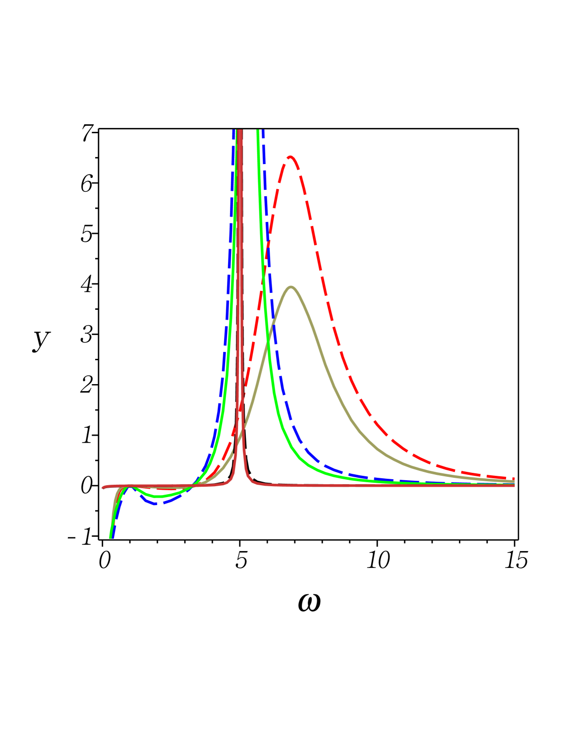
It is observed that the polynomial is non-negative, while can be negative and so can ; the behaviors of are plotted in Fig. 1. Then it is easy to see that in the classical case, Eq. (23) reduces to regardless of the coupling strength . Likewise, we also have the free energy expressed as
| (25) |
In comparison, Eq. (23a) identically vanishes in an isolated case; however, for the aforementioned reason, we have indeed in this case. Therefore, we may say that the smoothness of the distribution (24) reflects the system-bath coupling.
To observe explicitly how the system-bath coupling strength affects both energies and , we apply to (23a) the identity obtained from the interplay between generalized functions and the theory of moments KAN04 such that
| (26) |
Here the symbol denotes the th derivative, and the th moment with the Heaviside step function . Then, with the aid of (21), the formal decomposition (26) can explicitly be evaluated as
where the moments are given by and
| (3a) | ||||
| (3b) |
It is easy to verify that in the weak-coupling limit , all moments where . The substitution of (3) into (23) then allows us to have
| (28) |
where the summation on the right-hand side reflects all system-bath coupling. An expression with the same structure immediately follows for the free energy , too.
It is a noteworthy fact that as a simple case, we have at zero temperature, and so Eq. (25) can be rewritten as a reduced expression with [cf. (13a)]. Therefore, it looks like a free energy of the Hamiltonian which is in an isolated pure state; there is no heat flow between system and bath at zero temperature. On the other hand, the system-of-interest is in a mixed state due to the system-bath coupling even at zero temperature [cf. (2) and (12)]. This also suggests to us that the free energy cannot exactly be associated with the reduced system alone.
Similarly to (23), we next introduce another distribution which is useful for describing the the internal energy beyond the weak-coupling. By using (9) with , we can easily get
| (29) |
where the distribution
| (29a) |
reducing to in the identically vanishing coupling. Within the Drude-Ullersma model, we have KIM07
| (30) |
directly obtained from (22). Here the coefficients
| (30a) | |||
satisfy the relations
| (30b) | |||
which will be useful below. In the weak-coupling limit , we easily get
| (30c) |
Eqs. (8a) and (8b) can then be expressed explicitly as KIM07
| (31) | |||||
in terms of the digamma function , respectively, thus immediately giving the internal energy in its closed form. Here we also used the relation ABS74 . From this, we can easily verify that in the classical limit , the internal energy regardless of the coupling strength .
Now we substitute (30) with (30b) into (29a), which will yield
| (32) | |||||
Therefore, the distribution is non-negative. It is easy to verify the normalization for . The behaviors of are displayed in Fig. 2. In comparison, Eq. (32) identically vanishes in an isolated case; however, likewise with , we have indeed in this case. We can also obtain, as the counterpart to (3),
| (33) | |||||
where the moments are given by and
| (33a) | ||||
| (33b) |
In the weak-coupling limit , all moments where . The substitution of (33) into (29) can immediately give rise to the sum rule for , which is the counterpart to (28). In addition, we stress that the probability density is not a quantum-mechanical quantity.
Next we intend to express the distribution in terms of , which will enable us to relate the thermodynamic energy directly to thermodynamic quantities of the reduced system . We first compare (24) and (32), which easily leads to with
| (34) | |||||
It is also straightforward to verify that . In the Ohmic limit, Eq. (34) vanishes. Then we can get
| (35) |
By substituting this into (23) and then applying Eqs. (2) and (29), we can finally arrive at the expression
| (36) |
where the coupling-induced term (cf. Appendix A)
| (36a) | ||||
| (36b) | ||||
It can be shown that this vanishes indeed with . This also vanishes in the classical limit . Eq. (36b) is displayed in Fig. 3.
Similarly, the free energy can also be expressed as
| (37) |
where a generalized “free energy” , and
| (37a) | ||||
| (37b) | ||||
expressed in terms of the gamma function . It can be shown that Eq. (37b) vanishes with , as well as with . Fig. 4 displays different behaviors of (37b).
Now we consider the free energy change . This turns out to be identical to the quantum-mechanical average value
| (38) |
evaluated along an isothermal process, i.e., in the infinitesimally slow variation of frequency (cf. Appendix B). However, this “work” may conceptually not be interpreted as a minimum average work performed on the reduced system , due to the fact that the actual average work should be defined as an average value of a classical stochastic variable with transition probabilities derived from quantum mechanics, rather than as an expectation value of some “work” operator TAL07 ; accordingly, the minimum average work comes out when the individual work of each run is performed only for the reversible process.
Next let us discuss the second law of thermodynamics within the system-of-interest in terms of and . To do so, we reinterpret an entire process as a sum of the following three sub-processes, based on the fact that all thermodynamic state functions are path-independent; in the sub-process (I), we completely decouple the system oscillator from a bath by letting the non-vanishing coupling strengths in an isothermal fashion. The internal energy change through this first sub-process is given by while the free energy change needed for decoupling the system from the bath, FOR06 ; KIM06 ; KIM07 . In the next sub-process (II) we vary the frequency of the resultant isolated oscillator according to the pre-determined protocol, followed by its coupling weakly to the bath which makes the oscillator come back to the thermal equilibrium at temperature . The relevant internal energy change and free energy change are and , respectively. In this sub-process, the JE (1) holds true. In the last sub-process (III) we increase the coupling strengths up to their original values in an isothermal fashion; the internal energy change , and the free energy change needed for coupling the system to the bath, . As a result, the total internal energy change and free energy change through sub-processes (I)-(III) equal and , respectively.
We remind that the inequality is valid (so is ), particularly in the low-temperature regime KIM07 ; FOR06 ; KIM06 . Therefore, this inequality says that if we consider a next decoupling process after (III) and then identified the free change with the (maximum) useful work spontaneously releasable from the coupled system , then the second law within the system could be violated. This tells us that the free energy change cannot be the (minimum) actual work performed on the system beyond the weak-coupling limit, and so the JE (17a) is not allowed to associate itself directly with the second law within the coupled oscillator.
Comments deserve here. From Eqs. (29) and (36)-(37) it is tempted to rewrite the internal energy as in terms of a generalized partition function beyond the weak-coupling limit, and the resultant “free energy” as , with . In the classical case, on the other hand, Eq. (37a) vanishes, and so indeed, explicitly given by
| (39) |
It is also notable that Eq. (39) is independent of , whereas this is not true for . This means that the classical free energy can be conceptually rescued only when the system-bath coupling is reflected (cf. of course, with , independent of ). This free energy will be employed below for our discussion of a generalized Jarzynski equality.
4 Quantum Jarzynski equality beyond the weak-coupling limit
We will introduce a generalized Jarzynski equality consistent with the second law within the oscillator coupled to a bath at an arbitrary strength. This will need an appropriate definition of the work performed on the system. Therefore we first consider a reversible process in which it is straightforward to evaluate the work. Then the generalized free energy change in the variation of frequency can be expressed as
| (40) |
where . From this, a generalized Jarzynski equality (GJE) beyond the weak-coupling limit is introduced as
| (41) |
where the average is carried out with the work distribution in (18) for an isolated oscillator in the frequency variation , as well as the probability density reflects the actual coupling between and .
In an isolated case the GJE easily reduces to the known form (1). As shown in (41), we now need to deal with a sum of the Jarzynski equalities, each being valid for an isolated system, with the initial and final “weights” and obtained directly from the susceptibility (cf. Appendix B). Technically this means that we first turn off the coupling , which makes the initial reduced density matrix (2) reduce to the canonical thermal state ; next we carry out the JE processes independently for many different frequencies ’s with the two weights. From this, we can extract the free energy change , without a measurement of any other “work” directly on the coupled system. It is instructive to remind that the JE (17a) can also be rewritten as
| (42) |
in its form, where the distributions ’s come from the susceptibility as well [cf. (23a) and (25)], but not guaranteed to be non-negative.
Next, in order to observe explicitly the deviation of the GJE from the JE in its known form, we substitute the sum rule (33) into (41), which yields
Therefore we can now look into the sufficiently weak, but not necessarily vanishingly small, coupling regime, simply by adding the low-order coupling-induced terms (33a) and (33b). On the other hand, beyond the weak coupling limit we cannot simply neglect higher-order moments (cf. Fig. 5 as well as Figs. 1, 2). As a result, we may say that the JE (1) is exactly valid only in the vanishingly small coupling limit.
Now we briefly discuss (4) in the classical limit . Then the term with easily reduces to
| (44) |
non-vanishing indeed. Likewise, so are all terms with . Therefore, even the classical JE (1) does not exactly hold true any longer beyond the weak-coupling limit.
It is also instructive to add remarks on the effect of system-bath coupling to the Jarzynski equality (41); in an isolated case, albeit the JE in its known form is well-known, we cannot perform an isothermal process, in which the (minimum) average work exactly amounts to the free energy change. And in an isothermal process we might think heat exchange through the system-bath coupling at every single moment in such a way that we switch off the coupling (“decoupling”) and then perform the external perturbation in the resultant isolated case, followed by contacting with the bath again (“coupling”); so the total heat exchange over the actual isothermal process would be equivalent to the amount of final thermal relaxation leading to the end equilibrium state in the above picture a pair of decoupling and coupling is added to. However, as discussed after (38), this picture could lead to a violation of the second law, and so is not acceptable. Moreover, in order to make the JE useful, the system under consideration needs to be sufficiently small-scaled, in which the work fluctuations are observable; in this scale, however, the system-bath coupling is normally non-negligible. As a result, we may argue that the usefulness of the JE in its known form is fairly limited.
Now we discuss the relevance of the GJE to the second law of thermodynamics within the system-of-interest beyond the weak-coupling limit. We first introduce the average work in an irreversible process as
| (45) |
where each partial average work is explicitly given by [cf. (19)]. As such, the average work , being not a quantum-mechanical expectation value, can be determined without any measurement of the work directly on the system coupled to a bath. Applying the Jensen inequality to (41), we can then obtain an expression of the second law of thermodynamics beyond the weak-coupling
| (46) |
equivalent to . It is now needed to ask if this equality is valid indeed; Figs. 6-7 demonstrate its validity for many different sets of parameters . Subsequently, the first law allows us to have the heat .
Lastly, a couple of short comments deserve here. First, we remind that our approach was made entirely in the local picture , rather than the total picture . Accordingly, there is no room appropriate for detecting system-bath entanglement directly within our generalized Jarzynski equality, while it was discussed, on the other hand, within the Jarzynski equality (17a) in VED10 . Secondly, in practical terms the number of independent experimental runs needed for obtaining a sufficiently visible convergence of the JE (1) grows exponentially with the system size GRO05 , and so the computational cost is high enough. This cost will be even higher when we deal with a system beyond the weak-coupling limit, due to the additional averaging needed for the GJE. Further it was shown GON13 that a significantly faster convergence of the JE can be achieved via accelerated adiabatic control. Even in this scheme the computational cost is expected to increase beyond the weak-coupling limit, from our result.
5 Concluding remarks
In summary, we derived a generalized Jarzynski equality in the scheme of a time-dependent quantum Brownian oscillator within the Drude-Ullersma damping model. This equality is associated with the second law of thermodynamics (in its generalized form) within the system oscillator coupled to a bath at an arbitrary strength. This finding also enables us to look systematically into the coupling effect on the non-equilibrium thermodynamics of the local system-of-interest beyond the weak-coupling limit. As a result, the Jarzynski equality in its original form (and all other relevant fluctuation theorems) was shown to be valid only in the vanishingly small coupling limit, which fact also holds true in the classical limit of .
We believe that our finding will provide a useful starting point for derivation of a generalized Jarzynski equality associated with the second law in more generic quantum dissipative systems. In fact, if a smooth probability density, such as in (29), reflecting the system-bath coupling is explicitly available, this derivation becomes conceptually rather a straightforward issue, while the technical procedure for an exact evaluation of such a probability density would be a formidable task for a broad class of nonlinear systems.
Acknowledgments
The author thanks G. Mahler (Stuttgart), G.J. Iafrate (NC State), and J. Kim (KIAS) for helpful remarks. He also acknowledges financial support provided by the U.S. Army Research Office (Grant No. W911NF-13-1-0323).
Appendix A : Detailed derivation of Eq. (36b)
Appendix B : Evaluation of Eq. (38)
We begin with [cf. (4a)]
| (50) |
at every single frequency value . With the aid of (8a) and , it turns out that
| (51) | |||||
Next, with the aid of (21) we can express the susceptibility (30) in terms of as , where
| (52) | |||
Substituting this into (51), we can finally obtain
| (53) | |||||
where , and
| (53a) | ||||
Using the relation GRA07
| (54) |
where , we can arrive at the expression
| (55) | |||
(note that ). By integration by parts, this can be transformed into
| (56) |
where the distribution
| (56a) | |||
| (56b) |
Here we also used both and the fact that Eq. (24a) can be rewritten in terms of as
| (57) | |||||
References
- (1) C. Jarzynski, Phys. Rev. Lett. 78, 2690 (1997).
- (2) H. B. Callen, Thermodynamics and an introduction to thermostatics, 2nd ed. (John Wiley, New York, 1985).
- (3) C. Jarzynski, Eur. Phys. J. B 64, 331 (2008).
- (4) E. Boksenbojm, B. Wynants, and C. Jarzynski, Physica A 389, 4406 (2010).
- (5) G. E. Crooks, J. Stat. Phys. 90, 1481 (1998).
- (6) G. E. Crooks, Phys. Rev. E 60, 2721 (1999).
- (7) C. Jarzynski, What is the microscopic response of a system driven far from equilibrium?, in Lecture Notes in Physics 597 (Springer, Berlin, 2002), pp 63-82.
- (8) J. Liphardt, S. Dumont, S. B. Smith, I. Tinoco Jr, and C. Bustamante, Science 296, 1832 (2002).
- (9) C. Bustamante, J. Liphardt, and F. Ritort, Phys. Today 58 (7), 43 (2005).
- (10) E. G. D. Cohen and D. Mauzerall, J. Stat. Mech. (2004) P07006.
- (11) C. Jarzynski, J. Stat. Mech. (2004) P09005.
- (12) H. Tasaki, arXiv:cond-mat/0009244 (2000).
- (13) S. Mukamel, Phys. Rev. Lett. 90, 170604 (2003).
- (14) W. De Roeck and C. Maes, Phys. Rev. E 69, 026115 (2004).
- (15) M. Esposito and S. Mukamel, Phys. Rev. E 73, 046129 (2006).
- (16) P. Talkner, E. Lutz, and P. Hänggi, Phys. Rev. E 75, 050102(R) (2007).
- (17) J. Teifel and G. Mahler, Phys. Rev. E 76, 051126 (2007).
- (18) A. Engel and R. Nolte, Eur. Phys. Lett. 79, 10003, (2007).
- (19) G. E. Crooks, J. Stat. Mech. (2008) P10023.
- (20) D. Andrieux and P. Gaspard, Phys. Rev. Lett. 100, 230404 (2008).
- (21) S. Deffner and E. Lutz, Phys. Rev. E 77, 021128 (2008).
- (22) P. Talkner, M. Campisi, and P. Hänggi, J. Stat. Mech. (2009) P02025.
- (23) J. Teifel and G. Mahler, Eur. Phys. J. B. 75, 275 (2010).
- (24) J. Teifel and G. Mahler, Phys. Rev. E 83, 041131 (2011).
- (25) V. A. Ngo and S. Haas, Phys. Rev. E 86, 031127 (2012).
- (26) D. P. Sheehan, Quantum limits to the second law, AIP Conf. Proc. 643 (AIP, Melville, NY, 2002).
- (27) J. Gemmer, M. Michel, and G. Mahler, Quantum Thermodynamics (Springer, Berlin, 2004).
- (28) C. Vladislav and D. P. Sheehan, Challenges to the second law of thermodynamics: theory and experiment (Springer, New York, 2005).
- (29) M. Campisi, P. Talkner, and P. Hänggi, Phys. Rev. Lett. 102, 210401 (2009).
- (30) M. Campisi, P. Talkner, and P. Hänggi, J. Phys. A 42, 392002 (2009).
- (31) G.-L. Ingold, Dissipative quantum systems, in Quantum transport and dissipation (Wiley-VCH, Weinheim, 1998), pp 213-248.
- (32) U. Weiss, Quantum dissipative systems, 3rd ed. (World Scientific, Singapore, 2008).
- (33) H. Grabert, P. Schramm, and G.-L. Ingold, Phys. Rep. 168, 115 (1988).
- (34) I. Kim and G. Mahler, Phys. Rev. E 81, 011101 (2010).
- (35) G. W. Ford, J. T. Lewis, and R. F. O’Connell, Ann. Phys. (N.Y.) 185, 270 (1988).
- (36) A. M. Levine, M. Shapiro, and E. Pollak, J. Chem. Phys. 88, 1959 (1988).
- (37) G. W. Ford, J. T. Lewis, and R. F. O’Connell, Phys. Rev. Lett. 55, 2273 (1985).
- (38) G. W. Ford and R. F. O’Connell, Physica E 29, 82 (2005).
- (39) P. Hänggi and G.-L. Ingold, Chaos 15, 026105 (2005).
- (40) P. Hänggi and G.-L. Ingold, Acta Phys. Pol. B 37, 1537 (2006).
- (41) G. W. Ford and R. F. O’Connell, Phys. Rev. Lett. 96, 020402 (2006).
- (42) I. Kim and G. Mahler, Eur. Phys. J. B 54, 405 (2006).
- (43) I. Kim and G. Mahler, Eur. Phys. J. B 60, 401 (2007).
- (44) G.-L. Ingold, Eur. Phys. J. B 85, 30 (2012) and references therein.
- (45) R. M. Wilcox, J. Math. Phys. 8, 962 (1967).
- (46) P. Ullersma, Physica 32, 27, 56, 74, 90 (1966).
- (47) To verify the normalization conditions for and , we apply to Eqs. (23a) and (32), respectively.
- (48) R. P. Kanwal, Generalized Functions: Theory and Applications, 3rd ed. (Birkuäuser, Boston, 2004).
- (49) M. Abramowitz and I. Stegun, Handbook of Mathematical Functions with Formulas, Graphs, and Mathematical Tables (Dover, New York, 1974).
- (50) J. Hide and V. Vedral, Phys. Rev. A 81, 062303 (2010).
- (51) R. C. Lua and A. Y. Grosberg, J. Phys. Chem. B 109, 6805 (2005).
- (52) J. Deng, Q. Wang, Z. Liu, P. Hänggi, and J. Gong, Phys. Rev. E 88, 062122 (2013).
- (53) I.S. Gradshteyn and I.M. Ryzhik, Table of Integrals, Series, and Products, 7th ed. (Academic Press, San Diego, 2007).
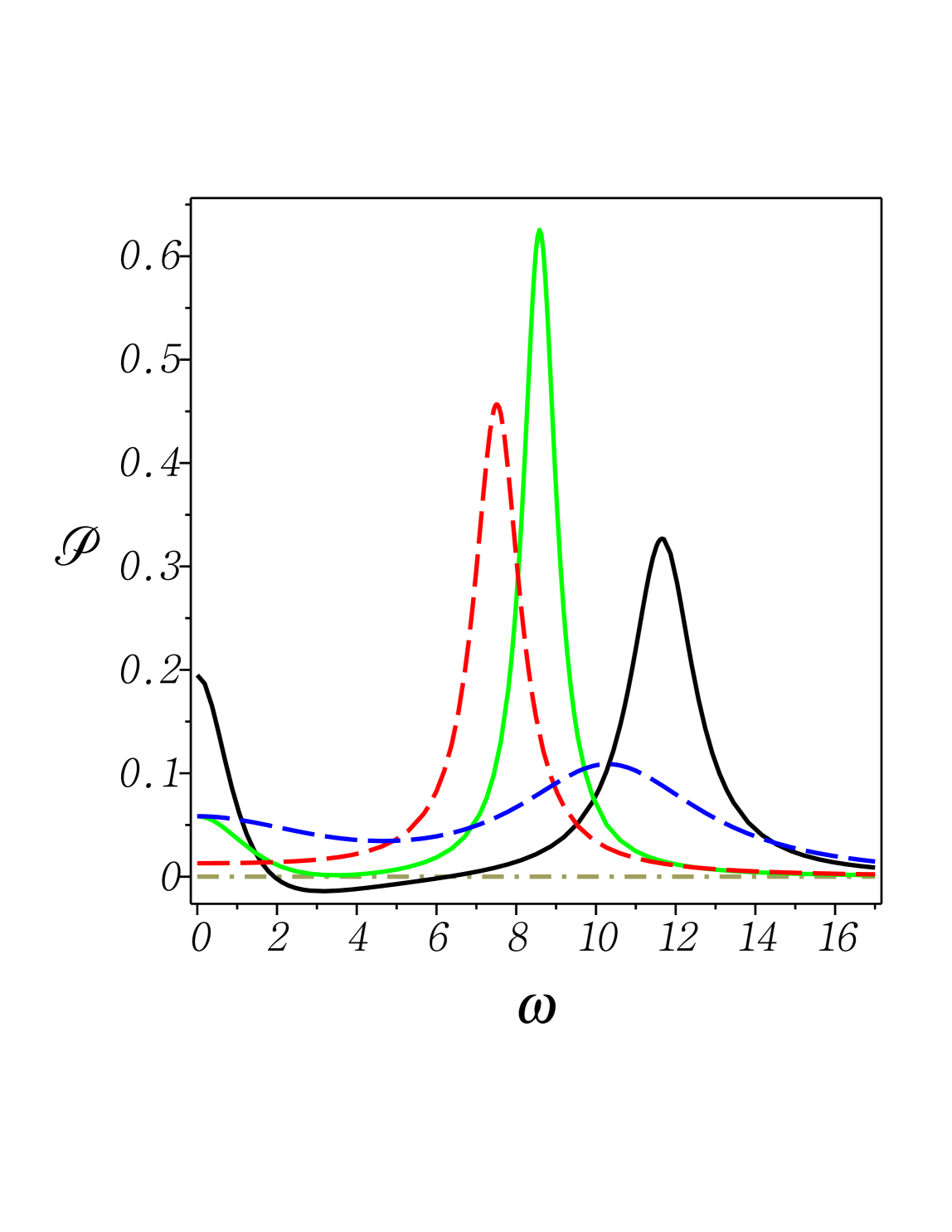
Fig. 1: (Color online) The distribution given in (24). Here we set . (I) Solid lines with , from top to bottom in the maximum values, 1st) green: ; 2nd) black: (can be negative). (II) Dash lines with , likewise, 1st) red: ; 2nd) blue: , in comparison with (khaki dashdot); cf. with .
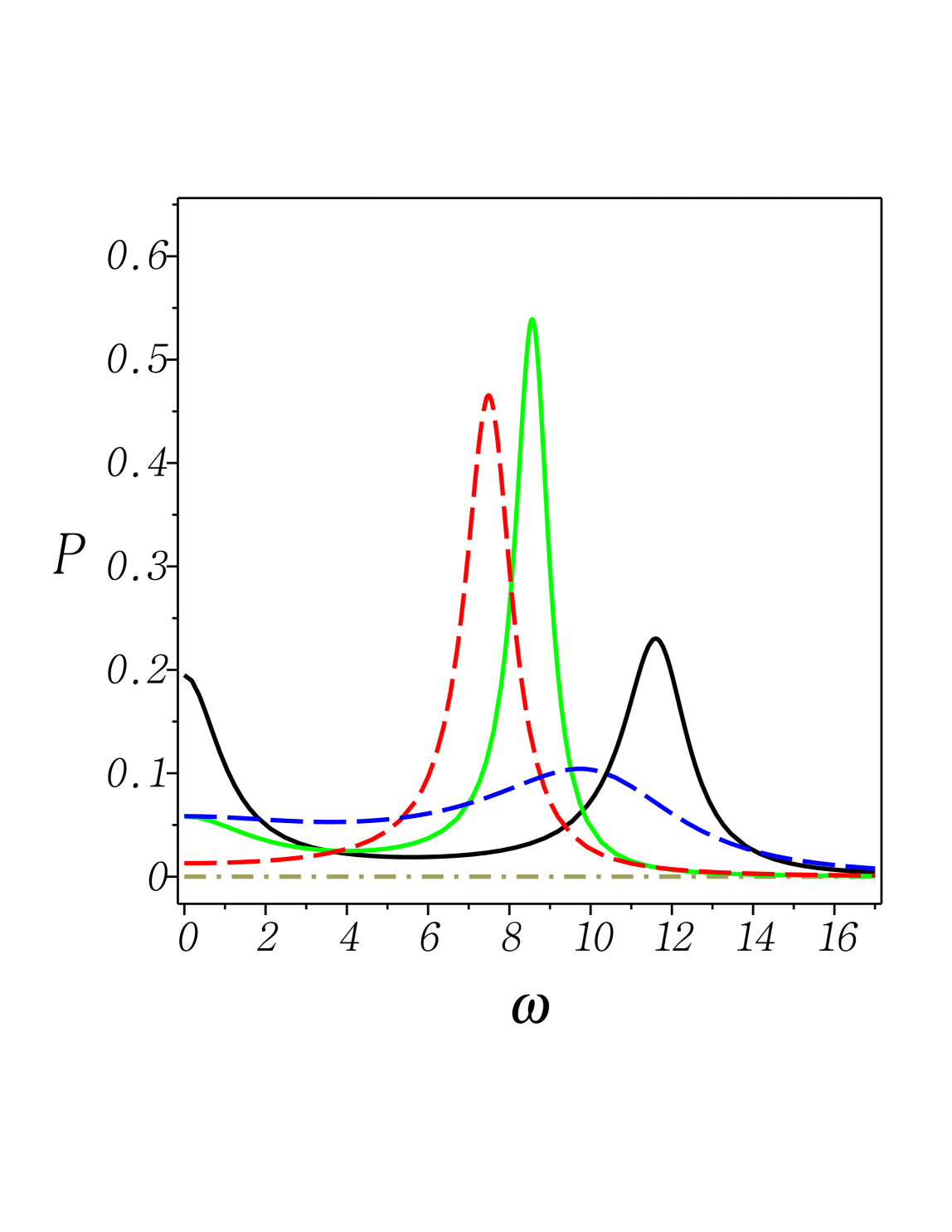
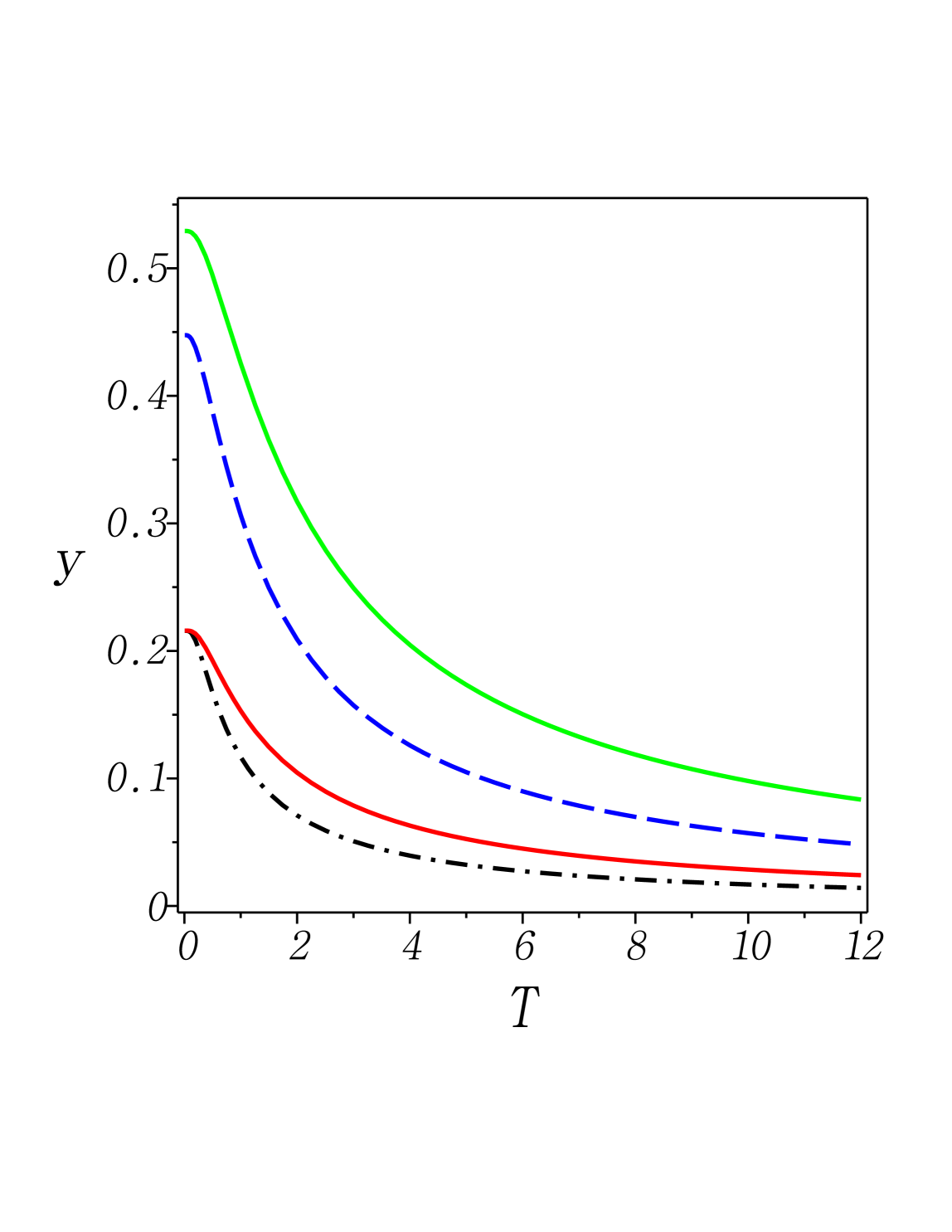
Fig. 3: (Color online) The dimensionless energy given in (36b) with versus dimensionless temperature . Here we set . From top to bottom, 1st) green solid: and (overdamped); 2nd) blue dash: and (overdamped); 3rd) red solid: and (underdamped); 4th) black dashdot: and (underdamped); here “overdamped” means whereas “underdamped” , after (21). With , .
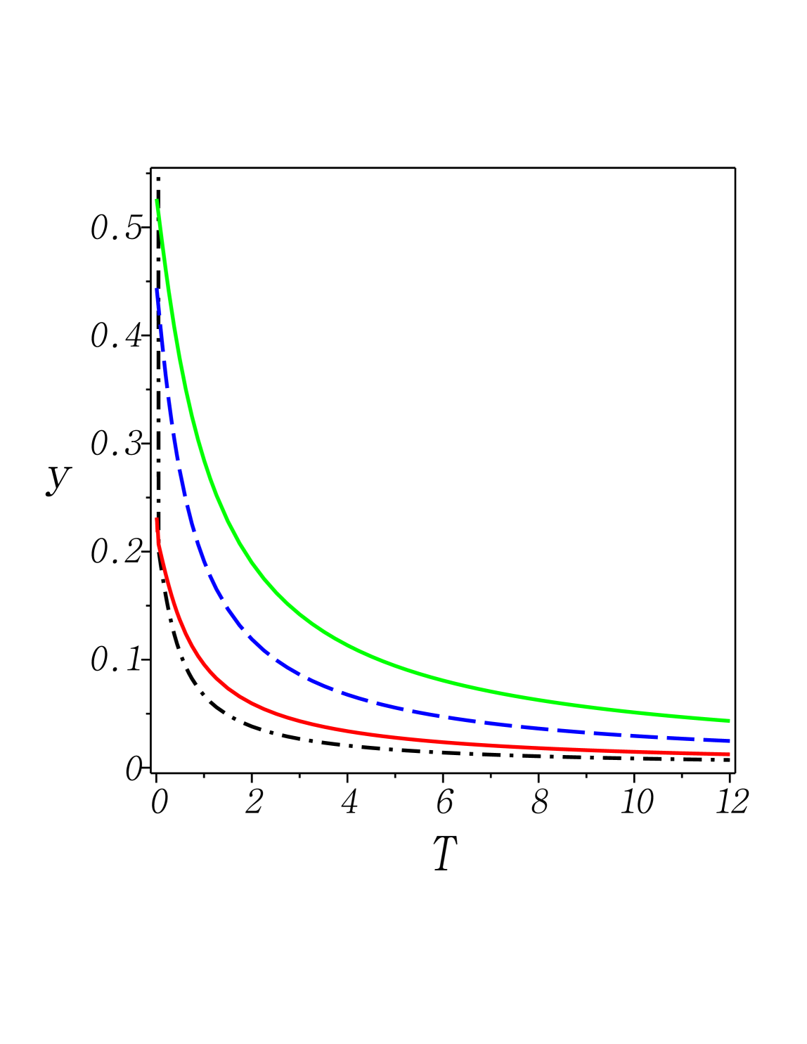
Fig. 4: (Color online) The dimensionless free energy given in (37b) with versus dimensionless temperature . The same as in Fig. 3.
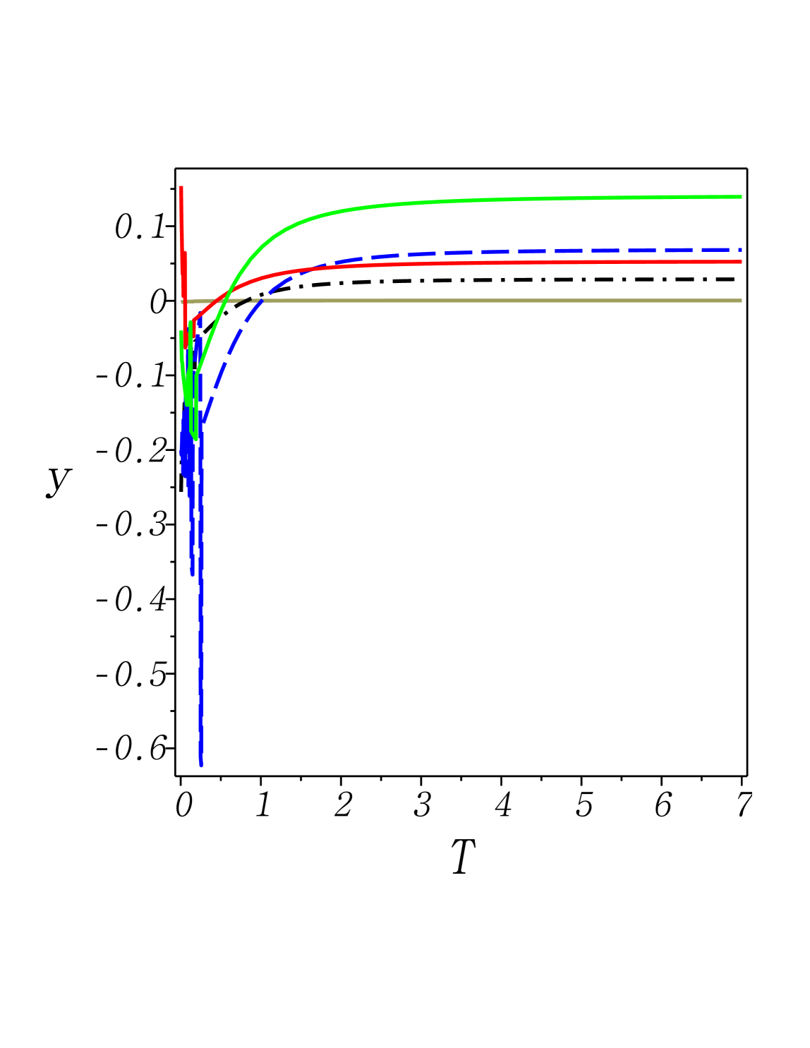
Fig. 5: (Color online) The relative error given in (4) versus dimensionless temperature , with being the leading term on the right-hand side of (4). Here we set and . From top to bottom at , 1st) green solid: and (strong-coupling limit); 2nd) blue dash: and (Ohmic and strong-coupling limit); 3rd) red solid: and (weak-coupling limit); 4th) black dashdot: and (Ohmic and weak-coupling limit); 5th) khaki solid: and (Ohmic and vanishingly small coupling limit).
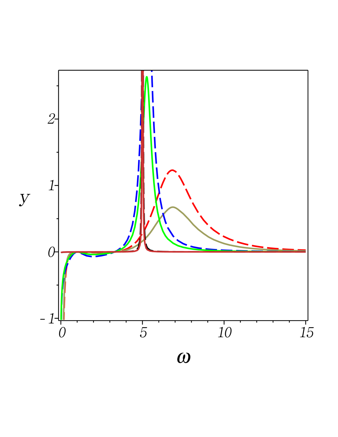
Fig. 6: (Color online) The dimensionless quantity given in (46) versus dimensionless frequency . Here we set and , and , as well as (low-temperature regime). Let . (I) Solid lines with the duration (slow change), 1st) orange, with a peak at : (vanishingly small coupling) and ; 2nd) green, with maximum value shifted a little to the right: and ; 3rd) grey, with maximum value shifted further to the right: (strong coupling) and . (II) Dash lines with (fast change), in the same way as in (I), 1st) black: ; 2nd) blue: ; 3rd) red: . As demonstrated, (1) the smaller , the larger -value, i.e., is an irreversibility measure of the process; (2) the -value can be negative-valued due to its factor , however, the integral is non-negative.