Joint and Individual Component Regression
Abstract
Multi-group data are commonly seen in practice. Such data structure consists of data from multiple groups and can be challenging to analyze due to data heterogeneity. We propose a novel Joint and Individual Component Regression (JICO) model to analyze multi-group data. In particular, our proposed model decomposes the response into shared and group-specific components, which are driven by low-rank approximations of joint and individual structures from the predictors respectively. The joint structure has the same regression coefficients across multiple groups, whereas individual structures have group-specific regression coefficients. Moreover, the choice of global and individual ranks allows our model to cover global and group-specific models as special cases. For model estimation, we formulate this framework under the representation of latent components and propose an iterative algorithm to solve for the joint and individual scores under the new representation. To construct the latent scores, we utilize the Continuum Regression (CR), which provides a unified framework that covers the Ordinary Least Squares (OLS), the Partial Least Squares (PLS), and the Principal Component Regression (PCR) as its special cases. We show that JICO attains a good balance between global and group-specific models and remains flexible due to the usage of CR. Finally, we conduct simulation studies and analysis of an Alzheimer’s disease dataset to further demonstrate the effectiveness of JICO. R implementation of JICO is available online at https://github.com/peiyaow/JICO.
Keywords: Continuum Regression; Heterogeneity; Latent Component Regression; Multi-group Data.
1 Introduction
Many fields of scientific research involve the analysis of heterogeneous data. In particular, data may appear in the form of multiple matrices, with data heterogeneity arising from either variables or samples. One example is the multi-view/source data, which measure different sets of variables on the same set of samples. The sets of variables may come from different platforms/sources/modalities. For instance, in genomics studies, measurements are collected as different biomarkers, such as mRNA and miRNA (Muniategui et al.,, 2013). Another example is the multi-group data, which measure the same set of variables on disparate sets of samples, which leads to heterogenous subpopulations/subgroups in the entire population. For instance, in the Alzheimer’s Disease (AD) study, subjects can have different subtypes, such as Normal Control (NC), Mild Cognitive Impairment (MCI), and AD.
We study the classical regression problem with one continuous response for multi-group data. Although there are many well-established regression techniques for homogeneous data (Hoerl and Kennard,, 1970; Tibshirani,, 1996), they may not be suitable for multi-group data. One naive approach is to ignore data heterogeneity and fit a global model using these techniques. However, a single global model can be too restrictive because the diverse information from different subgroups may not be identified. On the other hand, one can train separate group-specific models. Despite its flexibility, the information that is jointly shared across different groups is not sufficiently captured. Therefore, it is desirable to build a flexible statistical model that can simultaneously quantify the jointly shared global information and individual group-specific information for heterogeneous data.
There are several existing methods proposed in the literature under the context of regression for multi-group data. Meinshausen and Bühlmann, (2015) took a conservative approach and proposed a maxmin effect method that is reliable for all possible subsets of the data. Zhao et al., (2016) proposed a partially linear regression framework for massive heterogeneous data, and the goal is to extract common features across all subpopulations while exploring heterogeneity of each subpopulation. Tang and Song, (2016); Ma and Huang, (2017) proposed fused penalties to estimate regression coefficients that capture subgroup structures in a linear regression framework. Wang et al., (2018) proposed a locally-weighted penalized model to perform subject-wise variable selection. Wang et al., (2023) proposed a factor regression model for heterogeneous subpopulations under the high-dimensional factor decomposition. However, these models either are not specifically designed to identify the globally-shared and group-specific structures, or impose strong theoretical assumptions on the covariates. On the other hand, there exist some works that study this manner for multi-source data. Lock et al., (2013) proposed JIVE to learn joint and individual structures from multiple data matrices by low-rank approximations. Some extensions of JIVE can be found in Feng et al., (2018); Gaynanova and Li, (2019). All of these decomposition methods are fully unsupervised. Recently, Li and Li, (2021) proposed a supervised integrative factor regression model for mult-source data and studied its statistical properties with hypothesis tests. Palzer et al., (2022) proposed sJIVE that extends JIVE with the supervision from the response. These methods are supervised, but both focused on regressions for multi-source data.
In this paper, we consider the supervised learning problem of predicting a response with multi-group data. We propose a Joint and Individual COmponent Regression (JICO), a novel latent component regression model that covers JIVE as a special case. Our proposed model decomposes the response into jointly shared and group-specific components, which are driven by low-rank approximations of joint and individual structures from the predictors respectively. The joint structure shares the same coefficients across all groups, whereas individual structures have group-specific coefficients. Moreover, by choosing different ranks of joint and individual structures, our model covers global and group-specific models as special cases. To estimate JICO, we propose an iterative algorithm to solve for joint and individual scores using latent component representation. To construct the latent scores, we utilize the Continuum Regression (CR) (Stone and Brooks,, 1990), which provides a unified framework that covers OLS, PLS, and PCR as special cases. Some follow-up studies and modern extensions of CR can be found in Björkström and Sundberg, (1996); Lee and Liu, (2013). Embracing this flexibility and generaliziblity from CR, our proposed JICO model extends to the heterogeneous data setup and is able to achieve different model configurations on the spectrum of CR under this more complicated setting. JICO attains a good balance between global and group-specific models, and further achieves its flexibility by extending CR.
The rest of this paper is organized as follows. In Section 2, we briefly review JIVE and introduce our proposed JICO model. We further provide sufficient conditions to make JICO identifiable. In Section 3, after two motivating special cases, we introduce our iterative algorithm. In Sections 4 and 5, we evaluate the performance of JICO by simulation studies and real data analysis on the Alzheimer’s disease dataset, respectively. In Section 6, we conclude this paper with some discussion and possible extensions.
2 Motivation and Model Framework
Suppose we observe data pairs from groups, where and are the data matrix and the response vector for the th group respectively. In this setting, each data matrix has the same set of explanatory variables, whereas the samples vary across groups. We let and , where .
Our model is closely related to JIVE, which provides a general formulation to decompose multiple data matrices into joint and individual structures. The JIVE decomposes as
| (2.1) |
where represents the submatrix of the joint structure of , represents the individual structure of , and is the error matrix. We consider that has a similar decomposition into joint and individual signals
| (2.2) |
where is the noise from the -th group. Let and be the noiseless counterparts of and . Lemma 1 gives conditions to ensure that , , , and are identifiable.
Lemma 1
Given , where . There exists unique and such that and they satisfy the following conditions:
-
(i)
;
-
(ii)
, for ;
-
(iii)
.
Moreover, if , then there exists unique and such that and they satisfy and .
Lemma 1 shows that can be uniquely decomposed into the sum of and if we require them to satisfy conditions , following similar statements as in Feng et al., (2018). To ensure the unique decomposition of , we need to further require , which is different from Palzer et al., (2022), that requires .
In practice, only and are observable. In Lemma 2, we show in that the identifiable conditions in Lemma 1 can still be achieved given the observed . Moreover, in Lemma 2, we show that if and are assumed to have low ranks, they can be further decomposed as , where is a score matrix, is a loading matrix, and ; and , where is a score matrix and is a loading matrix, and . Under this formulation, if , then (2.1) and (2.2) can be expressed as
| (2.3) | |||
| (2.4) |
where and are the coefficients of the joint and individual components respectively. Model (2.4) gives a unified framework to model multi-group data. When , the joint term vanishes and (2.4) reduces to a group-specific model of . On the other hand, when , the individual term vanishes and (2.4) reduces to a global model of . When and , (2.4) has both global and group-specific components, thus lies between the above two extreme cases.
Lemma 2
Given , it holds that
-
(a)
There exists matrices and such that they satisfy conditions in Lemma 1 and .
-
(b)
There exists matrices such that and can be expressed as and , where . Moreover, there exists and which can be expressed as and , where and , with .
Corollary 1
There exist matrices and such that and defined by , , and as in Lemma 2 satisfy conditions in Lemma 1 and , if and , for all .
Corollary 1 follows directly from the proof of Lemma 2. As a remark, the columns of and form the sets of bases that span the row spaces of and respectively. Hence, is a sufficient and necessary condition for . Moreover, note that in Lemma 2, directly implies that , the latter being a sufficient condition for . Therefore, in Corollary 1, provides a sufficient condition for , which satisfies one of the identifiability constraints for the unique decomposition of in Lemma 1. In Section 3, we describe the algorithm to solve for and respectively.
3 Model Estimation
The key to estimate (2.3) and (2.4) is the constructions of score matrices and . To motivate our estimation procedure, in Sections 3.1, we discuss the joint and individual score estimation under two special cases respectively. In Section 3.2, we introduce an iterative algorithm for the general case.
3.1 Joint and Individual Score Estimation
We first consider a special case that . Under this setup, the individual components vanish and (2.3) and (2.4) reduce to the following model:
| (3.1) |
where , , and .
The formulation of (3.1) covers many existing classic methods. For example, in PCR, is chosen to be the score matrix of the first principal components of . However, PCR is inherently unsupervised and ignores the information from . Among the other supervised methods, PLS regression is a popular approach that incorporates regression on the latent scores. When and , the standard OLS can also be cast under the above setup.
According to the proof of our Lemma 2, can be constructed with the basis matrix . For the estimation of , we utilize the continuum regression (CR) (Stone and Brooks,, 1990) algorithm, the result of which covers OLS, PLS, and PCR as special cases. For , CR sequentially solves from the following optimization problem:
| (3.2) | ||||
| s.t. |
where and , once columns of and are centralized to have mean zero. Here, is a tuning parameter that controls how much variability of is taken into account for the construction of . When , the objective function in (3.2) is dominated by and does not play a role. The CR solution of then seeks to find the principal component directions that maximize the variation of . It can be shown that (3.2) coincides with OLS and PLS solutions when and respectively.
Let denote the solution to (3.2) and . Then can be estimated by As illustrated in Lemma 2, is the projection of onto the column space spanned by . Hence, we have , which further gives .
Next we consider our model estimation under the special case that . In this case, the joint component vanishes, and (2.3) and (2.4) reduce to the following individual model:
| (3.3) |
Same as the above discussion for joint score estimation, we utilize CR to construct as linear transformation of , where is a basis matrix, whose columns span . Let . Given group , for , CR sequentially solves from the following optimization problem:
| (3.4) | ||||
| s.t. | ||||
Denote the solution to (3.4). Similar to the joint estimation, once is constructed, can be obtained as the least square solution: Afterwards, we can have and .
3.2 JICO Algorithm
In this section, we consider the general case where or can be both nonzero. Since solving (3.2) and (3.4) simultaneously can be hard with both joint and individual structures specified in the full model (2.3) and (2.4), we propose to iteratively solve one of them while fixing the other. This leads to the following iterative procedure.
-
•
Given , solve the following constrained problem sequentially for :
(3.5) s.t. -
•
Given , for any , solve the following constrained problem sequentially for :
(3.6) s.t. -
•
Repeat the above two procedures until convergence.
Note that in (3.5) and (3.6), we denote
and Moreover, the last two constraints in (3.5) and (3.6) correspond to the two sufficient conditions in Corollary 1 to satisfy the identifiability conditions and needed in Lemma 1.
We formulate (3.5) and (3.6) into a generic CR problem, and derive an algorithm to solve it in Appendix B. Furthermore, we describe the convergence criterion for the iterative procedure and give its pseudo code in Algorithm 1 of Appendix C. Empirically, the algorithm always meets our convergence criteria, albeit there are no theoretical guarantees. In practice, we recommend starting the algorithm with multiple initial values and choose the one with the smallest cross-validated mean squared error. To predict the response using JICO estimates, we let and , where is the test set. Then, the prediction of response is given by .
In practice, we need to select tuning parameters , and . We describe how to select the tuning parameters in Appendix D. Since we use a grid search for tuning parameters, if the difference between the ranks of individual matrices and joint matrix are large, our algorithm may take a long time to compute. The goal of our algorithm is to approximate the joint and individual structure of the data by some low-rank matrices, and use the resulting low-rank matrices for prediction. Therefore, when the individual matrices and joint matrix are too complex and can not be approximated by some low-rank matrices, we suggest to use alternative methods to solve the problem.
Finally, we point out that our method includes JIVE-predict (Kaplan and Lock,, 2017) as a special case. JIVE-predict is a two-stage method that implements JIVE on first and then regresses the responses on the loading matrix. When we let in (3.2) and (3.4), JICO is equivalent as performing JIVE on . For that reason, our method in that case is equivalent to JIVE-predict.
4 Simulation Studies
One significant advantage of our proposed model is its flexibility of lying in between global and group-specific models. Moreover, the choice of parameter in CR allows it to identify the model that best fits the data. In this section, we conduct multiple simulation studies to further demonstrate the advantage of our proposed model.
We consider three simulation settings in this section. In the first two settings, we generate data according to models that contain both global and group-specific components. The data are generated in a way that PCR and PLS solutions are favored respectively. In the last setting, we simulate data from two special cases: a global model and a group-specific model. The data are simulated so that the OLS is favored for both cases. For all three settings, JICO can adaptively choose the correct model parameter so that it has the optimal performance. Moreover, we further illustrate how the rank selection impacts the performance of JICO by examining the results using mis-specified ranks.
We fix . In each replication, we generate 100 training samples to train the models and evaluate the corresponding Mean Squared Error (MSE) in an independent test set of 100 samples. We repeat simulations for 50 times.
For , we generate as i.i.d. samples from . For the sake of simplicity, we generate by the following model with two latent components:
| (4.1) |
where is the joint latent score vector with an coefficient , is the individual latent score vector with an coefficient , and is generated as i.i.d. samples from . Here, and are all vectors, and they are constructed such that . We vary the choices of , , , and , which will be discussed later.
4.1 PCR Setting
In this section, we simulate the model which favors . In this case, CR solutions to (3.2) and (3.4) coincide with PCR, which are essentially the top eigenvectors of the corresponding covariance matrices.
To simulate this setup, given training data , we let be the top eigenvector corresponding to . We further set as the top eigenvector of , where is the data matrix after projecting into the linear subspace that is orthogonal to . This projection ensures that the construction of and satisfies . To generate , we let .
We train JICO on a wide range of , using different combinations of , with a maximum of iterations. Figure 4.1(a) demonstrates the MSEs evaluated on the test data over repetitions. For better illustration, we plot MSE curves as a function of , with , which is a one-to-one monotone map from to . In particular, when and , we have and , which correspond to the cases of OLS, PLS and PCR respectively. The solid curve demonstrates the model performance given true ranks , whereas the gray curves show the performance of models with mis-specified ranks. In particular, we consider four mis-specified rank combinations. Among them, two rank combinations (, ; , ) correspond to joint models. The other two combinations (, ; , ) correspond to group-specific models. We can see from Figure 4.1(a) that the absolute minimum is given by the model with true ranks and , which refers to the underlying true model. When we look at the curves on the spectrum of as a whole, the joint models with or , always perform worse than the model with , because they are unable to capture the group-specific information from the underlying model. The model with true ranks performs better than the individual models with , or for larger values of , because the latter models cannot capture as much global information as the former. However, the model with performs worse than the individual models for smaller values of , where the latter achieves much more acceptable performances. This means that the choice of optimal ranks for our model can be sensitive to the choice of . For smaller values, individual models tend to be more reliable under the PCR setting. We notice that the end of the curve is not very smooth when . One possible reason is that the solution path of CR can sometimes be discontinuous with respect to (Björkström and Sundberg,, 1996), consequently the CR algorithm may be numerically unstable for certain values.
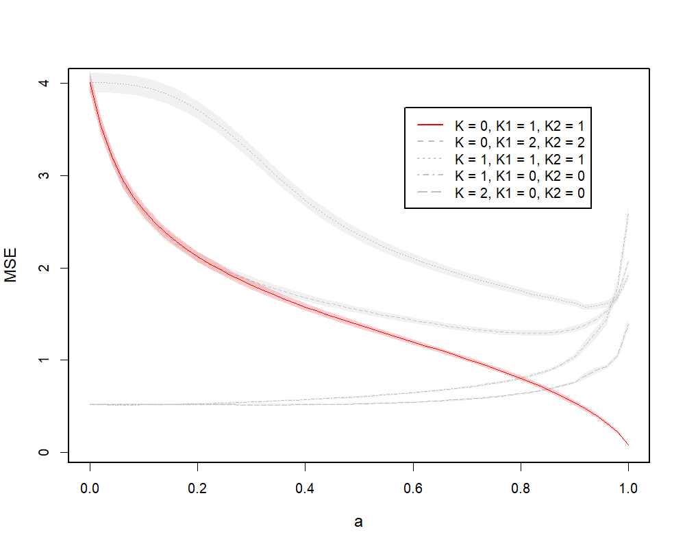
(a) PCR Example
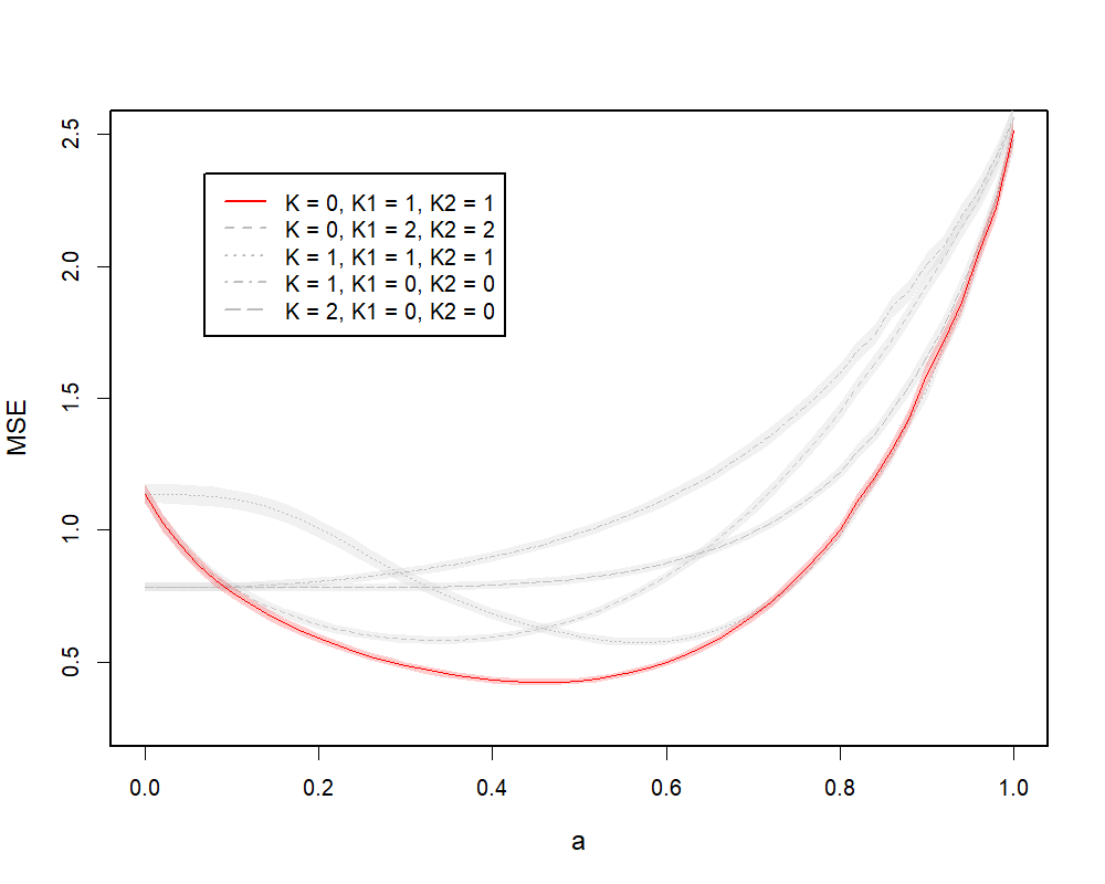
(b) PLS Example
We further illustrate the performance of JICO by comparing it with several existing methods. In particular, we include ridge regression (Ridge), partial least squares (PLS) and principal component regression (PCR). For JICO, we select the models trained under true ranks (performance as illustrated by the solid curve in Figure 4.1(a), with , which correspond to the cases of OLS, PLS and PCR respectively. For a fair comparison, for PLS and PCR methods, we fix the number of components to be for both a global fit and a group-specific fit. Table 1(a) summarizes the MSEs and of these methods. The numbers provided in the brackets represent the standard error. The first two columns summarize the performance for each group (), and the last column summarizes the overall performance. The JICO model with performs significantly better than the rest, because it agrees with the underlying true model. Among other mis-specified methods, group-specific PLS is relatively more robust to model mis-specification.
| Method | Overall | ||||
|---|---|---|---|---|---|
| (a) PCR Example | JICO | 1.994(0.063) | 2.012(0.068) | 2.003(0.053) | |
| 0.679(0.018) | 0.701(0.026) | 0.69(0.017) | |||
| 0.04(0.001) | 0.04(0.001) | 0.04(0.001) | |||
| Global | Ridge | 1.734(0.056) | 1.78(0.065) | 1.757(0.052) | |
| PLS | 1.163(0.033) | 1.194(0.045) | 1.178(0.031) | ||
| PCR | 0.946(0.04) | 0.977(0.044) | 0.961(0.022) | ||
| Group-specific | Ridge | 0.252(0.009) | 0.27(0.009) | 0.261(0.005) | |
| PLS | 0.254(0.009) | 0.272(0.009) | 0.263(0.005) | ||
| PCR | 0.68(0.042) | 0.71(0.05) | 0.695(0.032) | ||
| (b) PLS Example | JICO | 0.57(0.023) | 0.567(0.021) | 0.569(0.018) | |
| 0.211(0.008) | 0.218(0.008) | 0.215(0.006) | |||
| 1.236(0.038) | 1.277(0.037) | 1.256(0.025) | |||
| Global | Ridge | 1.698(0.064) | 1.742(0.06) | 1.72(0.055) | |
| PLS | 0.3(0.011) | 0.297(0.01) | 0.299(0.008) | ||
| PCR | 1.229(0.036) | 1.298(0.041) | 1.263(0.025) | ||
| Group-specific | Ridge | 0.375(0.013) | 0.425(0.016) | 0.4(0.01) | |
| PLS | 0.412(0.014) | 0.406(0.016) | 0.409(0.008) | ||
| PCR | 1.234(0.037) | 1.25(0.036) | 1.242(0.024) | ||
| (c) OLS Example (a) | JICO | 0.082 (0.002) | 0.083 (0.003) | 0.082 (0.002) | |
| 0.403 (0.011) | 0.419 (0.011) | 0.411 (0.007) | |||
| 1.006 (0.031) | 1.07 (0.03) | 1.038 (0.02) | |||
| Global | Ridge | 0.084 (0.004) | 0.084 (0.003) | 0.084 (0.003) | |
| PLS | 0.221 (0.007) | 0.226 (0.006) | 0.223 (0.005) | ||
| PCR | 0.991 (0.032) | 1.069 (0.030) | 1.030 (0.020) | ||
| Group-specific | Ridge | 0.574 (0.017) | 0.599 (0.024) | 0.586 (0.013) | |
| PLS | 0.572 (0.016) | 0.599 (0.024) | 0.585 (0.013) | ||
| PCR | 0.996 (0.032) | 1.061 (0.030) | 1.028 (0.021) | ||
| (d) OLS Example (b) | JICO | 0.063(0.002) | 0.066(0.004) | 0.064(0.002) | |
| 0.257(0.009) | 0.27(0.009) | 0.264(0.006) | |||
| 1.004(0.031) | 1.002(0.03) | 1.003(0.023) | |||
| Global | Ridge | 0.646(0.021) | 0.673(0.024) | 0.66(0.019) | |
| PLS | 0.957(0.027) | 0.971(0.032) | 0.964(0.022) | ||
| PCR | 1.023(0.031) | 1.016(0.031) | 1.019(0.023) | ||
| Group-specific | Ridge | 0.076(0.004) | 0.072(0.005) | 0.074(0.003) | |
| PLS | 0.113(0.003) | 0.116(0.005) | 0.115(0.003) | ||
| PCR | 0.978(0.03) | 0.987(0.029) | 0.983(0.022) | ||
4.2 PLS Setting
In this section, we consider the model setup that is more favorable to . In this scenario, the CR solutions to (3.2) and (3.4) coincide with the PLS solutions. Same as in Section 4.1, we still consider the construction of weights as linear transformations of the eigenvectors.
Given training data , denote as the matrix of top eigenvectors of . We let , where denotes a vector with elements all equal to . In this way, the top eigenvectors contribute equally to the construction of . Similarly, we let and be the matrix of top eigenvectors of . Then we let . To construct a model more favorable to PLS, in this section, we let and . We generate from (4.1) by letting and .
Similar to the PCR setting, in Figure 4.1(b), we illustrate the MSE curves of JICO models with different rank combinations on a spectrum of , where . Again, the solid curve represents the model with true ranks, while the gray curves represent models with mis-specified ranks. The absolute minimum is given by the solid curve at around , which corresponds to the underlying true model. Moreover, the solid curve gives almost uniformly the best performance on the spectrum of compared with the gray curves, except on a small range of close to . Hence, under the PLS setting, the optimal ranks can be less sensitive to the choice of . At initial values of , the solid curve almost overlaps with the gray curve that represents the joint model with . This means that when is close to , the individual signals identified by the full model with can be ignored. Therefore, the two group-specific models that capture more individual information give the best performance in this case. For values closer to , the gray curve that represents the joint model with is very close to the solid curve. This means that the effects of individual components estimated by JICO tend to become more similar across groups for larger .
In Table 1(b), we summarize the MSEs of JICO models trained with true ranks and , along with other methods as described in Section 4.1. JICO with shows the best performance among all methods, followed by the global PLS method, since the true model favors PLS and the coefficient for the group-specific component is relatively small.
4.3 OLS Setting
In this section, we simulate the setting that favors , which corresponds to the case of OLS in CR. It is shown in Stone and Brooks, (1990) that when , there is only one non-degenerate direction that can be constructed from the CR algorithm. Hence, under the JICO framework, the model that favors embraces two special cases: a global model with , and a group-specific model with , .
For the two cases, we simulate with (a) , and (b) , respectively. The construction of and is the same as that in Section 4.2 with and .
Figure 4.2 illustrates MSE curves of the two cases, where (a) represents the case of the global model and (b) represents the case of the group-specific model. In both cases, the absolute minimum can be found on the solid curves at , which represents the MSE curves from the models with true ranks and respectively. In (a), there are two competitive models against the model with true ranks: another global model with , and the model with . They both achieve the same performance with the solid curve at , and stay low at larger values of . This is because, when is mis-specified, additional model ranks help capture more information from data. The , model performs better because the underlying model is a global model. This is also true for (b). The global minimum can be found at on the solid curve, while the model performs better when gets larger. Again, this is because larger helps capture more information from data. The model does not perform as well, because the estimated joint information dominates, which does not agree with the true model. We observe some discontinuities on the curve, since the CR solution path can sometimes be discontinuous with respect to as discussed in the PCR setting in Section 4.1.
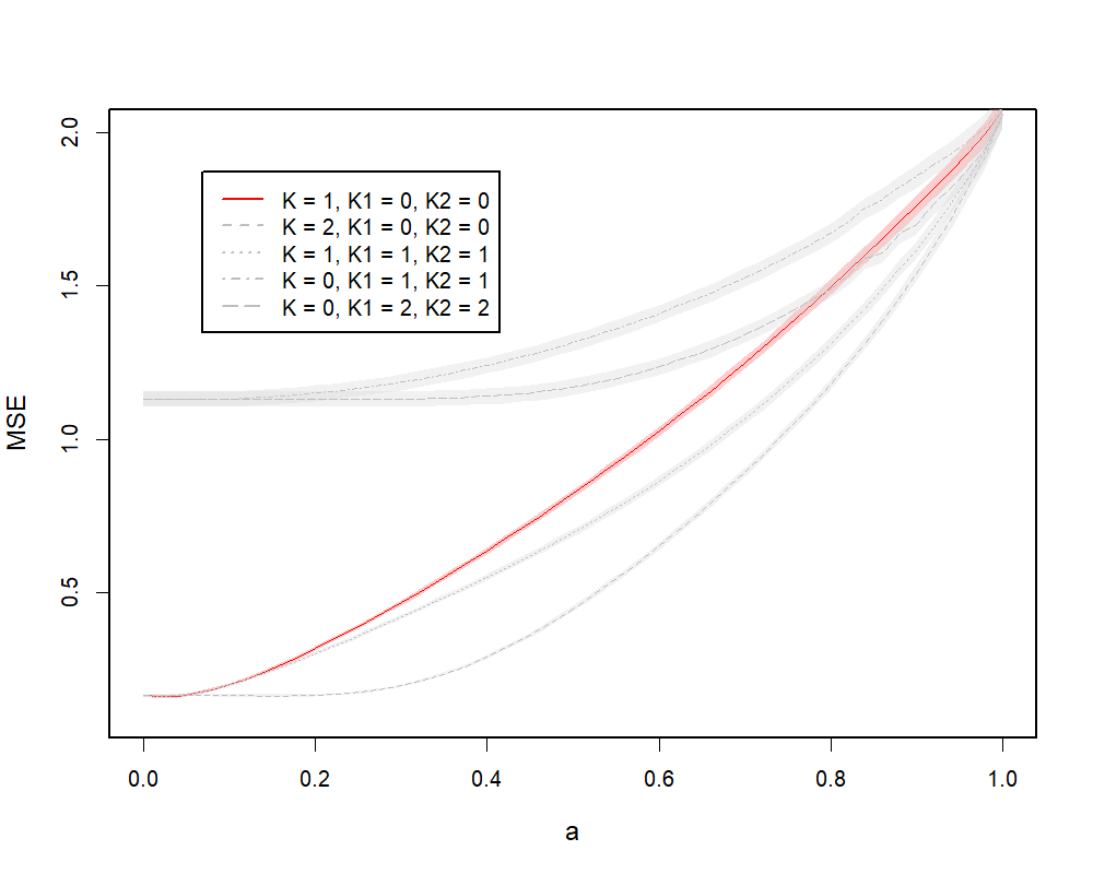
(a)
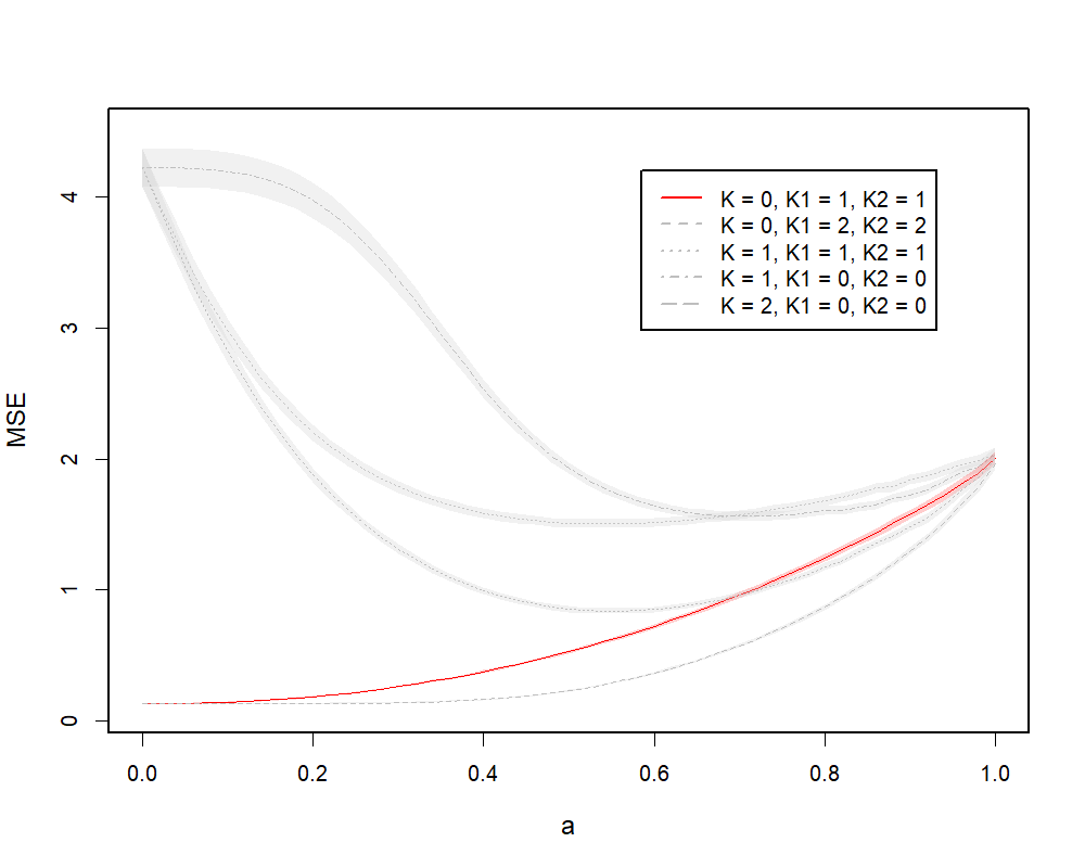
(b)
In Table 1 (c) and (d), we summarize the MSEs of JICO models trained with the true ranks with and other methods described in Section 4.1. For a fair comparison, the number of components for PCR and PLS is chosen to be for both global and group-specific fits. The JICO model with , along with Ridge always achieve better performance than all other methods. It is interesting to notice that in (c), the JICO models with and coincides with global PLS and PCR respectively, and hence they achieve the same performances. Similarly, in (d), JICO models with and coincide with group-specific PLS and PCR respectively, and they achieve the same performance correspondingly. In addition, when , the solution of CR algorithm coincides with the global OLS model. Thus the JICO model with and the global Ridge have similar performance in (c). Similarly, when , the JICO model with and group-specific Ridge have similar performance in (d).
5 Applications to ADNI Data Analysis
We apply our proposed method to analyze data from the Alzheimer’s Disease (AD) Neuroimaging Initiative (ADNI). It is well known that AD accounts for most forms of dementia characterized by progressive cognitive and memory deficits. The increasing incidence of AD makes it a very important health issue and has attracted a lot of scientific attentions. To predict the AD progression, it is very important and useful to develop efficient methods for the prediction of disease status and clinical scores (e.g., the Mini Mental State Examination (MMSE) score and the AD Assessment Scale-Cognitive Subscale (ADAS-Cog) score). In this analysis, we are interested in predicting the ADAS-Cog score by features extracted from 93 brain regions scanned from structural magnetic resonance imaging (MRI). All subjects in our analysis are from the ADNI2 phase of the study. There are 494 subjects in total in our analysis and 3 subgroups: NC (178), eMCI (178) and AD (145), where the numbers in parentheses indicate the sample sizes for each subgroup. As a reminder, NC stands for the Normal Control, and eMCI stands for the early stage of Mild Cognitive Impairment in AD progression.
For each group, we randomly partition the data into two parts: 80% for training the model and the rest for testing the performance. We repeat the random split for 50 times. The testing MSEs and the corresponding standard errors are reported in Table 2. Both groupwise and overall performance are summarized. We compare our proposed JICO model with four methods: ridge regression (Ridge), PLS, and PCR. We perform both a global and a group-specific fit for Ridge, PLS, and PCR, where the regularization parameter in Ridge and the number of components in PCR or PLS are tuned by 10-fold cross validation (CV). For our proposed JICO model, we demonstrate the result by fitting the model with fixed , or tuned respectively. In practice, using exhaustive search to select the optimal values for and can be computationally cumbersome, because the number of combinations grows exponentially with the number of candidates for each parameter. Based on our numerical experience, we find that choosing to be the same does not affect the performance on prediction too much. Details are discussed in Appendix D. Therefore, in all these cases, the optimal ranks for JICO are chosen by an exhaustive search in and to see which combination gives the best MSE. We choose and to be small to improve our model interpretations. The optimal value of is chosen by 10-fold CV.
As shown in Table 2, JICO performs the best among all competitors. Fitting JICO with yields the smallest overall MSE. JICO with parameters chosen by CV performs slightly worse, but is still better than the other global or group-specific methods. The results of JICO with and , which correspond to OLS, PLS, and PCR, are also provided in Table 2. Even though their prediction is not the best, an interesting observation is that they always have better performance than their global or group-specific counterparts. For example, when , JICO has much better overall prediction than the group-specific PLS. This indicates that it is beneficial to capture global and individual structures for regression when subpopulations exist in the data.
In Table 2, global models perform the worst, because they do not take group heterogeneity into consideration. The group-specific Ridge appears to be the most competitive one among group-specific methods. Note that for the AD group, our JICO model with or tuned outperforms the group-specific Ridge method by a great margin.
| Method | NC | eMCI | AD | Overall | |
|---|---|---|---|---|---|
| JICO | 6.671 (0.137) | 11.319 (0.309) | 55.798 (1.556) | 22.821 (0.466) | |
| 6.316 (0.121) | 10.394 (0.279) | 40.853 (1.294) | 17.951 (0.394) | ||
| 6.443 (0.124) | 10.353 (0.291) | 44.054 (1.449) | 18.929 (0.441) | ||
| 6.608 (0.138) | 11.121 (0.308) | 49.997 (1.832) | 21.013 (0.558) | ||
| CV | 6.414 (0.129) | 10.333(0.289) | 41.297 (1.348) | 18.096 (0.401) | |
| Global | Ridge | 23.450 (0.751) | 21.276 (0.796) | 63.989 (2.657) | 34.692 (0.840) |
| PLS | 26.310 (0.787) | 22.672 (0.915) | 68.193 (3.183) | 37.442 (0.982) | |
| PCR | 25.228 (0.771) | 21.966 (0.802) | 69.541 (2.969) | 37.209 (0.907) | |
| Group-specific | Ridge | 6.336 (0.116) | 10.353 (0.278) | 42.271 (1.315) | 18.364 (0.392) |
| PLS | 6.656 (0.136) | 11.298 (0.306) | 48.434 (1.725) | 20.629 (0.524) | |
| PCR | 6.656 (0.136) | 11.346 (0.304) | 47.357 (1.484) | 20.327 (0.454) | |
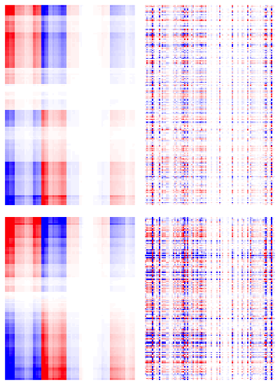
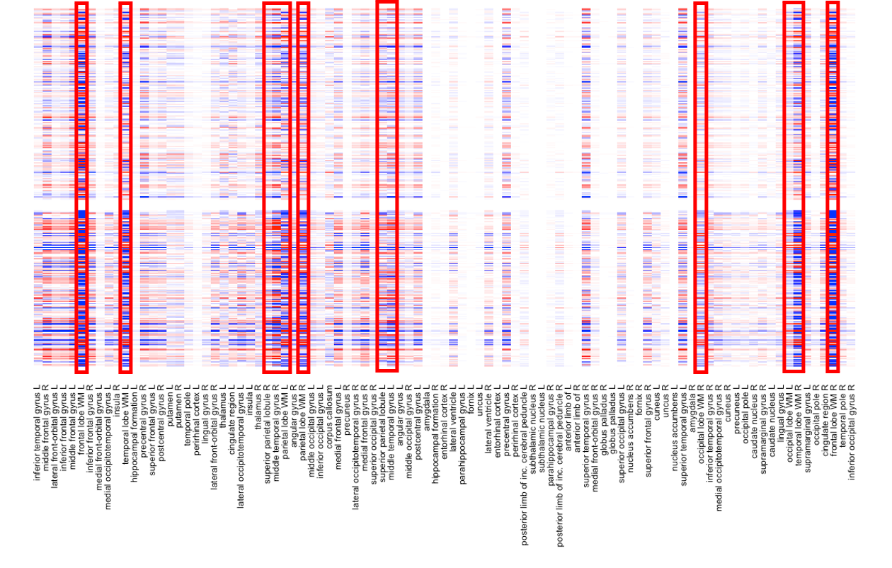
To get our results more interpretable, we further apply the JICO model to NC and AD groups. We run 50 replications of 10-fold CV to see which combination of tuning parameters gives the smallest overall MSE. The best choice is . Then, we apply JICO using this choice and tuning parameters and give the heatmaps of the estimated (left column) and (right column) in Figure 5.1. Rows of heatmaps represent samples and columns represent MRI features. We use the Ward’s linkage to perform hierarchical clustering on the rows of , and arrange the rows of and in the same order for each group. Moreover, we apply the same clustering algorithm to the columns of to arrange the columns in the same order across the two disease groups for both joint and individual structures. Figure 5.1 shows that JICO separates joint and individual structures effectively. The joint structures across different disease groups share a very similar pattern, whereas the individual structures appear to be very distinct. We further magnify the right column of Figure 5.1 in Figure 5.2 with the brain region names listed. We find that the variation in for the AD group is much larger than the counterpart for the NC group. We highlight the brain regions that differ the most between the two groups. The highlighted regions play crucial roles in human’s cognition, thus important in AD early diagnosis (Michon et al.,, 1994; Killiany et al.,, 1993). For example, Michon et al., (1994) suggested that anosognosia in AD results in part from frontal dysfunction. Killiany et al., (1993) showed that the temporal horn of the lateral ventricles can be used as antemortem markers of AD.
NC
AD

6 Discussion
In this paper, we propose JICO, a latent component regression model for multi-group heterogeneous data. Our proposed model decomposes the response into jointly shared and group-specific components, which are driven by low-rank approximations of joint and individual structures from the predictors respectively. For model estimation, we propose an iterative procedure to solve for model components, and utilize CR algorithm that covers OLS, PLS, and PCR as special cases. As a result, the proposed procedure is able to extend many regression algorithms covered by CR to the setting of heterogeneous data. Extensive simulation studies and a real data analysis on ADNI data further demonstrate the competitive performance of JICO.
JICO is designed to be very flexible for multi-group data. It is able to choose the optimal parameter to determine the regression algorithm that suits the data the best, so that the prediction power is guaranteed. At the same time, it is also able to select the optimal joint and individual ranks that best describe the degree of heterogeneity residing in each subgroup. The JICO application to ADNI data has effectively illustrated that our proposed model can provide nice visualization on identifying joint and individual components from the entire dataset without losing much of the prediction power.
DATA AVAILABILITY STATEMENT
The data that support the findings of this paper are available in the Alzheimer’s Disease Neuroimaging Initiative at https://adni.loni.usc.edu/.
Appendix A Proofs
Proof of Lemma 1. The proof of the first part of this lemma follows similar arguments as in Feng et al., (2018). Define . We assume that for non-trivial cases. For each , and can be obtained by projecting to and its orthogonal complement in . Thus, by construction, we have and . Since for all , we have , then has a zero projection matrix. Therefore, we have . On the other hand, since , the orthogonal projection of onto is unique. Therefore, the matrices and are uniquely defined.
For the second part of Lemma 1, note that . Then, and can be obtained by projecting onto and respectively. Because , and are uniquely defined.
Proof of Lemma 2. We explicitly describe how to find , , , , , , , to satisfy the requirements. First, can be obtained by finding an arbitrary set of bases that span . Then, can be obtained by solving a system of linear equations. We prove that such and satisfy conditions – in Lemma 1 and . Given and , we construct , so that they satisfy , and .
Let be an arbitrary set of bases that span . Denote . Let . Next, we show that satisfies condition in Lemma 1 for any . It suffices to show that , i.e. there exists , such that . Since the columns of form the bases of , there exists , such that . Then, we have . Let and , then we have
Given , we propose to solve
| (A.1) |
where is unknown. We first show that (A.1) has non-zero solutions. Since , (A.1) can be rewritten as where
Since
(A.1) has non-zero solutions.
Let be an arbitrary set of bases that spans the space of solutions to (A.1). Let Next we show that satisfies in Lemma 1 and . Since columns of satisfy (A.1), we have and . Then, by definition, and , which imply that and . Since for all , is perpendicular to the columns of , then we have .
Finally, letting , , and , we have . Let and , where . Then we obtain and by letting and .
Appendix B Derivation of the CR algorithm for solving (3.5) and (3.6)
Consider the following CR problem that covers (3.5) and (3.6) as special cases:
| (B.1) | ||||
| s.t. | ||||
where , , and are given a priori.
The solution to (S2) resides in , i.e. the space that is orthogonal to the columns of . Hence, we let and , the latter being the projection of into the space that is orthogonal to the columns of . Let be the rank of the matrix , and be the corresponding rank- SVD decomposition, with , , the diagonal matrix. Since the representation of the solution to (S2) might not be unique, to avoid ambiguity, we write the solution as the linear combination of the column vectors of , i.e. , for some . Note that all satisfies . Hence, the constraint from (S2) can be satisfied under this representation.
At step , the original optimization problem can be reformulated as follows:
| (B.2) |
where , and . To solve (B.2), we can expand the objective to its Lagrangian form:
where and are Lagrange multipliers. To solve (B.2), we take the derivative of with respect to , then the optimizer should be the solution to the following:
| (B.3) |
Left multiply to (B.3) and apply the constraints then we can conclude that . Plug this back to (B.3), and let and , then we have
A simple reformulation of the above plus the constraints yields the following matrix form:
| (B.4) |
where , , and . By the standard formula for inverse of a partitioned matrix and the constraint that , we obtain
| (B.5) |
where . Note that has a factor of and has a factor of , hence has a factor of that gets canceled out during the normalization in (B.5). Therefore, does not rely on the quantity of . Without loss of generality, we can choose . Then the only unknown parameter is . Hence, we can formulate (B.4) and (B.5) as a fixed point problem of as a function of . More specifically, we seek for that satisfies . Afterwards, we obtain , where and are computed from . We summarize the procedure to solve (B.2) as in the following two steps:
Step 1: Solve the fixed point for with , where
Step 2: Compute and from the fixed point in Step 2. The solution to (B.2) is then given by .
The most challenging step is Step 2, where a nonlinear equation needs to be solved. This can be done numerically by several existing algorithms. For example, we can use Newton’s method (Kelley,, 2003), which is implemented by many optimization packages and gives fast convergence in practice.
Appendix C JICO iterative algorithm
After each iteration, we obtain joint objective values as a vector:
| (C.1) |
and individual objective values as a vector for :
| (C.2) |
and compare them with the corresponding vectors obtained from the previous iteration step. Our iterative procedure stops until the differences between two consecutive iteration steps are under a certain tolerance level. Empirically, the algorithm always met convergence criteria, albeit there are no theoretical guarantees for it.
Appendix D Selection of Tuning Parameters
To apply the proposed JICO method, we need to select tuning parameters , and . Based on our numerical experience, we find that the performance of JICO depends more on the choice of but less on . We also find that even when the true differs in multiple groups, choosing them to be the same doesn’t affect the MSE in predicting the response too much. Thus, to saving computational time, we can choose to be the same for all groups. We propose to do an exhaustive search for and to find their best combination that gives the smallest MSE, where and are two user-defined constants. In this way, we need to try combinations in total. Since we assume and are both low-rank, we can set and to be relatively small. As for the tuning of , we propose to perform a grid search and choose the one that can minimize the MSE in predicting the responses.
Appendix E The impact of using different initial value
The following simulation study illustrates the impact of using different matrices as the initial value for our algorithm.
We use the same data generating scheme as described in Section 4. We fix . In each replication, we generate 100 training samples to train the models and evaluate the corresponding Mean Squared Error (MSE) in an independent test set of 100 samples. We also record the objective values as described below:
-
•
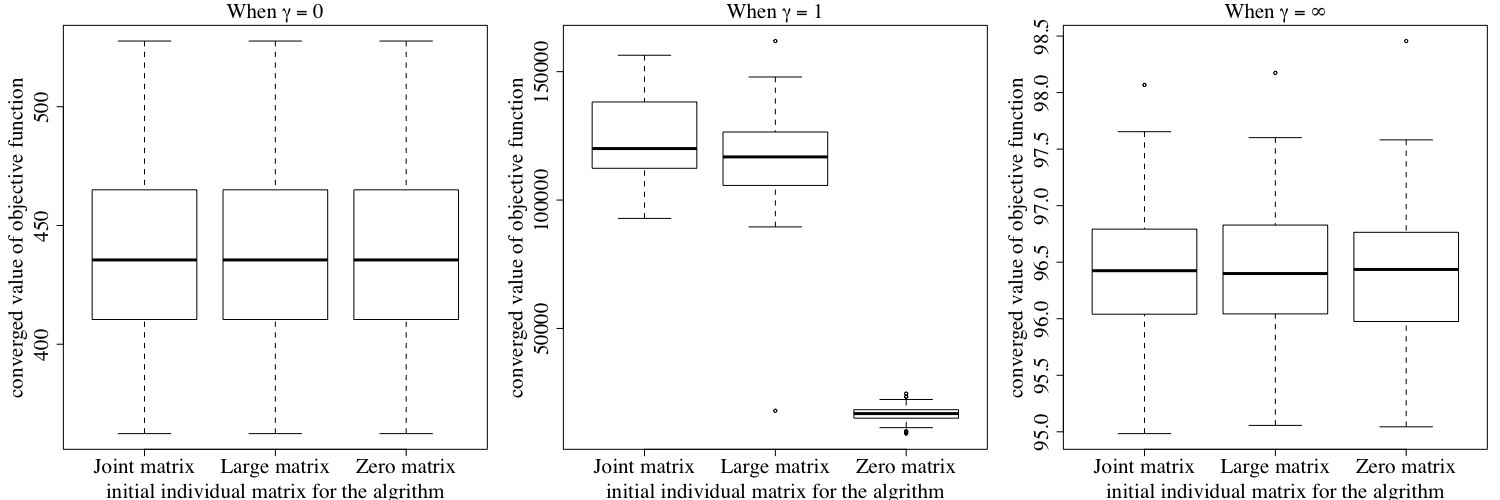
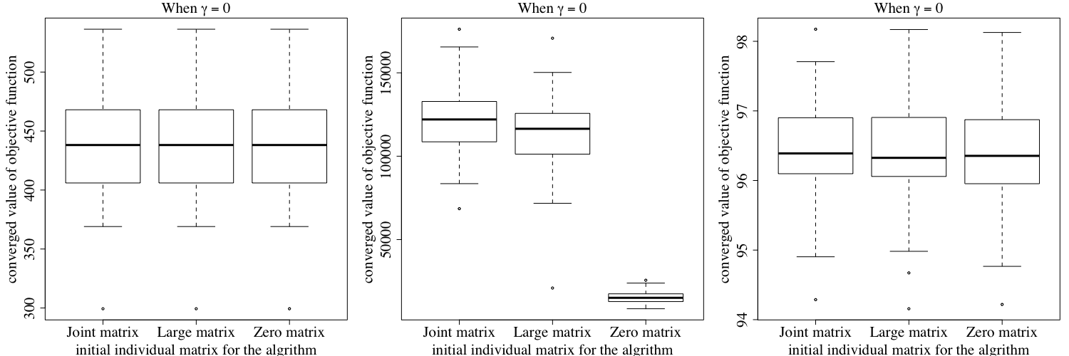
When , we compare the converged objective value as in (3.6) for .
-
•
When , we compare and for .
-
•
When , we compare and for .
We compare the performance of our algorithm by giving the boxplots of the MSEs and the converged objective values using different initial values. We repeat the simulation for 50 times, with three kinds of initial values of the individual matrices as follows:
-
•
Zero matrix: In this setting, our algorithm starts with zero matrices as the initial value, where all entries in are equal to 0.
-
•
Large matrix: In this setting, our algorithm starts with matrices with large entries as the initial value, where all entries in are equal to 3.
-
•
Joint matrix: In this setting, our algorithm starts with estimated joint matrices as the initial value, where are derived from our first setting, that is using zero matrices as the initial value.
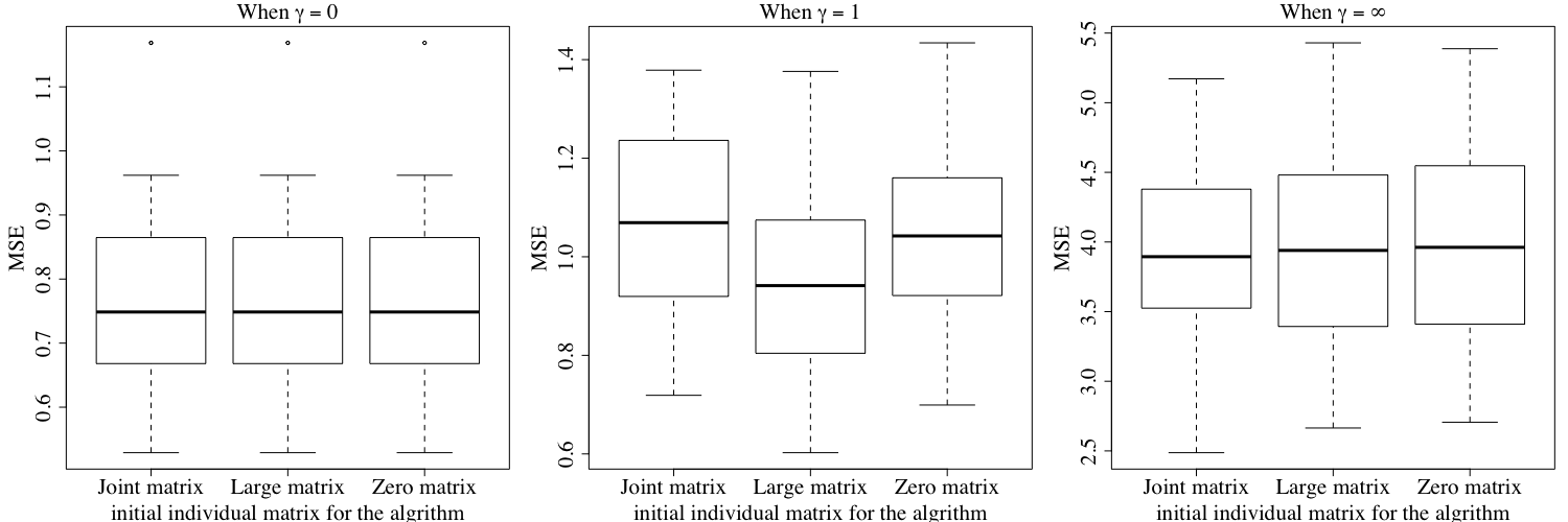
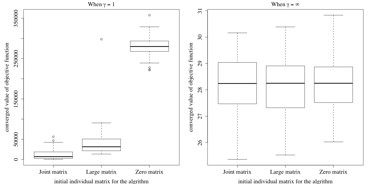
Figures E.2 shows the converged value of the joint objective function under the three different initial values of the individual matrices mentioned above. Similarly, Figure E.3 shows the converged value of the first objective function under the three different initial values. Finally, Figure E.4 shows the the converged value of the second individual objective function under three different initial values. The results show that our algorithm may not converge to the same objective function value using different initial values when , but Figure E.1 shows that our results tend to have a similar performance in terms of prediction error, no matter how we choose the initial individual matrices for our algorithm. To ensure a better performance, we recommend running our algorithm on the same dataset multiple times with different initial values, and then choose the result with the best performance.
References
- Björkström and Sundberg, (1996) Björkström, A. and Sundberg, R. (1996). Continuum regression is not always continuous. Journal of the Royal Statistical Society: Series B (Methodological), 58(4):703–710.
- Feng et al., (2018) Feng, Q., Jiang, M., Hannig, J., and Marron, J. (2018). Angle-based joint and individual variation explained. Journal of Multivariate Analysis, 166:241–265.
- Gaynanova and Li, (2019) Gaynanova, I. and Li, G. (2019). Structural learning and integrative decomposition of multi-view data. Biometrics, 75(4):1121–1132.
- Hoerl and Kennard, (1970) Hoerl, A. E. and Kennard, R. W. (1970). Ridge regression: Biased estimation for nonorthogonal problems. Technometrics, 12(1):55–67.
- Kaplan and Lock, (2017) Kaplan, A. and Lock, E. F. (2017). Prediction with dimension reduction of multiple molecular data sources for patient survival. Cancer Informatics, 16:1176935117718517.
- Kelley, (2003) Kelley, C. T. (2003). Solving nonlinear equations with Newton’s method, volume 1. Siam.
- Killiany et al., (1993) Killiany, R. J., Moss, M. B., Albert, M. S., Sandor, T., Tieman, J., and Jolesz, F. (1993). Temporal lobe regions on magnetic resonance imaging identify patients with early alzheimer’s disease. Archives of Neurology, 50(9):949–954.
- Lee and Liu, (2013) Lee, M. H. and Liu, Y. (2013). Kernel continuum regression. Computational Statistics and Data Analysis, 68:190–201.
- Li and Li, (2021) Li, Q. and Li, L. (2021). Integrative factor regression and its inference for multimodal data analysis. Journal of the American Statistical Association, pages 1–15.
- Lock et al., (2013) Lock, E. F., Hoadley, K. A., Marron, J. S., and Nobel, A. B. (2013). Joint and individual variation explained (jive) for integrated analysis of multiple data types. The Annals of Applied Statistics, 7(1):523–542.
- Ma and Huang, (2017) Ma, S. and Huang, J. (2017). A concave pairwise fusion approach to subgroup analysis. Journal of the American Statistical Association, 112(517):410–423.
- Meinshausen and Bühlmann, (2015) Meinshausen, N. and Bühlmann, P. (2015). Maximin effects in inhomogeneous large-scale data. The Annals of Statistics, 43(4):1801–1830.
- Michon et al., (1994) Michon, A., Deweer, B., Pillon, B., Agid, Y., and Dubois, B. (1994). Relation of anosognosia to frontal lobe dysfunction in alzheimer’s disease. Journal of Neurology, Neurosurgery and Psychiatry, 57(7):805–809.
- Muniategui et al., (2013) Muniategui, A., Pey, J., Planes, F. J., and Rubio, A. (2013). Joint analysis of mirna and mrna expression data. Briefings in Bioinformatics, 14(3):263–278.
- Palzer et al., (2022) Palzer, E. F., Wendt, C. H., Bowler, R. P., Hersh, C. P., Safo, S. E., and Lock, E. F. (2022). sjive: Supervised joint and individual variation explained. Computational Statistics & Data Analysis, 175:107547.
- Stone and Brooks, (1990) Stone, M. and Brooks, R. J. (1990). Continuum regression: cross-validated sequentially constructed prediction embracing ordinary least squares, partial least squares and principal components regression. Journal of the Royal Statistical Society: Series B (Methodological), 52(2):237–258.
- Tang and Song, (2016) Tang, L. and Song, P. X. (2016). Fused lasso approach in regression coefficients clustering: learning parameter heterogeneity in data integration. The Journal of Machine Learning Research, 17(1):3915–3937.
- Tibshirani, (1996) Tibshirani, R. (1996). Regression shrinkage and selection via the lasso. Journal of the Royal Statistical Society: Series B (Methodological), 58(1):267–288.
- Wang et al., (2023) Wang, P., Li, Q., Shen, D., and Liu, Y. (2023). High-dimensional factor regression for heterogeneous subpopulations. Statistica Sinica, 33:1–27.
- Wang et al., (2018) Wang, P., Liu, Y., and Shen, D. (2018). Flexible locally weighted penalized regression with applications on prediction of alzheimer’s disease neuroimaging initiative’s clinical scores. IEEE Transactions on Medical Imaging, 38(6):1398–1408.
- Zhao et al., (2016) Zhao, T., Cheng, G., and Liu, H. (2016). A partially linear framework for massive heterogeneous data. Annals of Statistics, 44(4):1400–1437.