Joint Bayesian component separation and CMB power spectrum estimation

H. K. Eriksen¹¹affiliation: email: h.k.k.eriksen@astro.uio.no ²²affiliation: Institute of Theoretical Astrophysics, University of Oslo, P.O. Box 1029 Blindern, N-0315 Oslo, Norway ³³affiliation: Centre of Mathematics for Applications, University of Oslo, P.O. Box 1053 Blindern, N-0316 Oslo , J. B. Jewell⁴⁴affiliation: Jet Propulsion Laboratory, California Institute of Technology, Pasadena CA 91109 , C. Dickinson⁴⁴affiliationmark: , A. J. Banday⁵⁵affiliation: Max-Planck-Institut für Astrophysik, Karl-Schwarzschild-Str. 1, Postfach 1317, D-85741 Garching bei München, Germany , K. M. Górski⁴⁴affiliationmark: ⁶⁶affiliation: Warsaw University Observatory, Aleje Ujazdowskie 4, 00-478 Warszawa, Poland , C. R. Lawrence⁴⁴affiliationmark:

(Received - / Accepted -)

Abstract

We describe and implement an exact, flexible, and computationally efficient algorithm for joint component separation and CMB power spectrum estimation, building on a Gibbs sampling framework. Two essential new features are 1) conditional sampling of foreground spectral parameters, and 2) joint sampling of all amplitude-type degrees of freedom (e.g., CMB, foreground pixel amplitudes, and global template amplitudes) given spectral parameters. Given a parametric model of the foreground signals, we estimate efficiently and accurately the exact joint foreground-CMB posterior distribution, and therefore all marginal distributions such as the CMB power spectrum or foreground spectral index posteriors. The main limitation of the current implementation is the requirement of identical beam responses at all frequencies, which restricts the analysis to the lowest resolution of a given experiment. We outline a future generalization to multi-resolution observations. To verify the method, we analyse simple models and compare the results to analytical predictions. We then analyze a realistic simulation with properties similar to the 3-yr WMAP data, downgraded to a common resolution of $3^{\circ}$ FWHM. The results from the actual 3-yr WMAP temperature analysis are presented in a companion Letter.

Subject headings:

cosmic microwave background — cosmology: observations — methods: numerical

1. Introduction

Great advances have been made recently both in experimental techniques for studying the cosmic microwave background (CMB) and in the measurements themselves. The angular power spectrum of temperature fluctuations has been characterized over more than three decades in angular scale (Hinshaw et al., 2007; Kuo et al., 2007; Readhead et al., 2004), and even the E-mode polarization spectrum has now been measured to some precision (Ade et al., 2007; Page et al., 2007; Montroy et al., 2006; Sievers et al., 2007). In the coming years, even greater improvements in sensitivity are expected, with the Planck nearing completion.

As the sensitivity of CMB experiments improves, the requirements on the control and characterization of systematic effects also increase. It is of critical importance to propagate properly the uncertainties caused by such effects through to the CMB power spectrum and cosmological parameters, in order not to underestimate the final uncertainties, and thereby draw incorrect cosmological conclusions.

A prime example of such systematic effects is non-cosmological foregrounds in the form of galactic and extra-galactic emission. With an amplitude rivaling that of the temperature signal over a significant fraction of the sky and completely dominating the polarization signal over most of the sky, the diffuse signal from our own galaxy must be separated accurately from the CMB signal in order not to bias the cosmological conclusions. Further, the uncertainties in the separation process must be propagated through to the errors on the CMB power spectrum and cosmological parameters.

These problems have been discussed extensively in the literature, and many different approaches to both power spectrum analysis and component separation have been proposed. Two popular classes of power spectrum estimation methods are the pseudo- $C_{\ell}$ estimators (e.g., Wright et al., 1994; Hivon et al., 2002; Szapudi et al., 2001) and maximum-likelihood methods (e.g., Górski, 1994, 1997; Bond et al., 1998). For a review and comparison of these methods, see Efstathiou (2004). Examples of component separation methods are the Maximum Entropy Method (Barreiro et al., 2004; Bennett et al., 2003b; Hobson et al., 1998; Stolyarov et al., 2002, 2005), the Internal Linear Combination method (Bennett et al., 2003b; Tegmark et al., 2003; Eriksen et al., 2004a), Wiener filtering (Bouchet & Gispert, 1999; Tegmark & Efstathiou, 1996), the Independent Component Analysis method (Maino et al., 2002, 2003; Donzelli et al., 2006; Stivoli et al., 2006), and direct likelihood estimation (Brandt et al., 1994; Górski et al., 1996; Banday et al., 1996; Eriksen et al., 2006).

The final step in a modern cosmological analysis pipeline is typically to estimate a small set of parameters for some cosmological model, which in practice is done by mapping out the parameter posteriors (or likelihoods) using an MCMC code (e.g., CosmoMC; Lewis and Bridle 2002). To do so, one must establish an expression for the likelihood $\mathcal{L}(C_{\ell})=P(\mathbf{d}|C_{\ell})$ , where $C_{\ell}$ is a theoretical CMB power spectrum and $\mathbf{d}$ are the observed data. It is therefore essential that the methods used in the base analysis pipeline (e.g., map making, component separation, power spectrum estimation) allow one to estimate this function both accurately and efficiently.

A particularly appealing framework for this task is the CMB Gibbs sampler, pioneered by Jewell et al. (2004) and Wandelt et al. (2004). While a brute-force CMB likelihood evaluation code must invert a dense signal-plus-noise covariance matrix, $\mathbf{C}=\mathbf{S}+\mathbf{N}$ , at a computational cost of $\mathcal{O}(N_{\textrm{pix}}^{3})$ , $N_{\textrm{pix}}$ being the number of pixels in the data set, the Gibbs sampler only requires the signal and noise covariance matrices separately. Consequently, the algorithmic scaling is dramatically reduced, typically to either $\mathcal{O}(N_{\textrm{pix}}^{3/2})$ or $\mathcal{O}(N_{\textrm{pix}}^{2})$ for data with white or correlated noise, respectively.

In addition to being a highly efficient CMB likelihood evaluator in its own right, as demonstrated by several previous analyses of real data (O’Dwyer et al., 2004; Eriksen et al., 2007a, b), the Gibbs sampler also offers unique capabilities for propagating systematic uncertainties end-to-end. Any effect for which there is a well-defined sampling algorithm, either jointly with or conditionally on other quantities, can be propagated seamlessly through to the final posteriors. One example of this is beam uncertainties. Given some stochastic description of the beam, for instance a mean harmonic space profile and an associated covariance matrix, one could sample at each step in the Markov chain one particular realization from this model and use the resulting beam for the next CMB sampling steps, allowing for a short burn-in period. The CMB uncertainties will then increase appropriately. Similar approaches could be taken for uncertainties in gain calibration and noise estimation.

However, rather than simply propagating a particular error term through the system, one often wants to estimate the characteristics of the effect directly from the data. In that case, a parametric model $P(\theta|\mathbf{d})$ , $\theta$ being a set of parameters describing the effect, must be postulated. Then, if it is both statistically and computationally feasible to sample from this distribution, the effect may be included in the joint analysis, and all joint posteriors will respond appropriately.

In this paper, we describe how non-cosmological frequency-dependent foreground signals may be included in a Gibbs sampler. In this framework the CMB signal is assumed Gaussian and isotropic, while the foregrounds are modeled either in terms of fixed spatial templates (e.g., monopoles, dipoles, low/high-frequency observations) or in terms of a free amplitude and spectral response function at each pixel. Our current code assumes identical angular resolution for all frequency bands, but we outline in §7 how the algorithm may be generalized to handle multi-resolution experiments.

Already with the present algorithm, we are able to perform a complete Bayesian joint CMB and foreground analysis of current CMB experiments on large angular scales. For example, in the present paper we demonstrate the algorithm on a realistic simulation corresponding to the 3-yr WMAP data. At an angular resolution of $3^{\circ}$ FWHM, we are able to produce the exact likelihood up to $\ell\sim 50$ -60, into the regime where a cruder likelihood description is likely to be acceptable (Eriksen et al., 2007a). Further, in a companion paper (Eriksen et al., 2007c) we analyze the real 3-yr WMAP data with the same tool, providing for the first time a complete set of physically motivated foreground posterior distributions of the observed microwave sky, together with their impact on cosmological parameters.

2. Review of basic algorithms

The algorithm developed in this paper is a essentially a hybrid of two previous algorithms, namely the CMB Gibbs sampler developed by Jewell et al. (2004), Wandelt et al. (2004) and Eriksen et al. (2004b), and the foreground MCMC sampler developed by Eriksen et al. (2006). In this section, we review these algorithms, emphasizing an intuitive and pedagogical introduction to the underlying ideas. In the next section we present the extensions required to make the hybrid code functional.

Note that while we discuss temperature measurements only in this paper, the methodology for analyzing polarization measurements is completely analogous. For example, see Larson et al. (2007) and Eriksen et al. (2007b) for details on polarized power spectrum analysis through Gibbs sampling.

2.1. The CMB Gibbs sampler

We first review the Gibbs sampler for CMB temperature measurements.

2.1.1 The CMB posterior

We choose our first data model to read

\mathbf{d}=\mathbf{s}+\mathbf{n},

(1)

where $\mathbf{d}$ are the observed data, $\mathbf{s}$ is the CMB sky signal, and $\mathbf{n}$ is instrumental noise. Complications such as multi-frequency observations and beam convolution will be introduced at a later stage.

We assume both the CMB signal and noise to be Gaussian random fields with vanishing mean and covariance matrices $\mathbf{S}$ and $\mathbf{N}$ , respectively. In harmonic space, where $\mathbf{s}=\sum_{\ell,m}a_{\ell m}Y_{\ell m}$ , the CMB covariance matrix is given by $\textrm{C}_{\ell m,\ell^{\prime}m^{\prime}}=\langle a_{\ell m}^{*}a_{\ell^{\prime}m^{\prime}}\rangle=C_{\ell}\delta_{\ell\ell^{\prime}}\delta_{mm^{\prime}}$ , $C_{\ell}$ being the angular power spectrum. The noise matrix $\mathbf{N}$ is left unspecified for now, but we note that for white noise it is diagonal in pixel space, $N_{ij}=\sigma_{i}^{2}\delta_{ij}$ , for pixels $i$ and $j$ and noise variance $\sigma^{2}_{i}$ .

Our goal is to estimate both the sky signal $\mathbf{s}$ and the power spectrum $C_{\ell}$ , which in a Bayesian analysis means to compute the posterior distribution $P(\mathbf{s},C_{\ell}|\mathbf{d})$ . By Bayes’ theorem, this distribution may be written as

	$\displaystyle P(\mathbf{s},C_{\ell}\|\mathbf{d})$	$\displaystyle\propto P(\mathbf{d}\|\mathbf{s},C_{\ell})P(\mathbf{s},C_{\ell})$		(2)
		$\displaystyle\propto P(\mathbf{d}\|\mathbf{s},C_{\ell})P(\mathbf{s}\|C_{\ell})P(C_{\ell}),$		(3)

where $P(C_{\ell})$ is a prior on $C_{\ell}$ , which we take to be uniform in the following. Our final power spectrum distribution may thus be interpreted as the likelihood, and integrated directly into existing cosmological parameter MCMC codes. Since we have assumed Gaussianity, the joint posterior distribution may thus be written as

P(\mathbf{s},C_{\ell}|\mathbf{d})\propto e^{-\frac{1}{2}(\mathbf{d}-\mathbf{s})^{t}\mathbf{N}^{-1}(\mathbf{d}-\mathbf{s})}\prod_{\ell}\frac{e^{-\frac{2\ell+1}{2}\frac{\sigma_{\ell}}{C_{\ell}}}}{C_{\ell}^{\frac{2\ell+1}{2}}}P(C_{\ell}),

(4)

where $\sigma_{\ell}\equiv\frac{1}{2\ell+1}\sum_{m=-\ell}^{\ell}|a_{\ell m}|^{2}$ is the angular power spectrum of the full-sky CMB signal.

2.1.2 Gibbs sampling

In principle, we could map out this distribution over a grid in $\mathbf{s}$ and $C_{\ell}$ , and the task would be done. Unfortunately, since the number of grid points required for such an analysis scales exponentially with the number of free parameters, this approach is not feasible.

A potentially much more efficient approach is to map out the distribution by sampling. However, direct sampling from the joint distribution in Equation 4 is difficult even from an algorithmic point of view alone; we are not aware of any textbook approach for this. And even if there were, it would most likely involve inverses of the joint $\mathbf{S}+\mathbf{N}$ covariance matrix, with a prohibitive $\mathcal{O}(N_{\textrm{pix}}^{3})$ scaling, in order to transform to the eigenspace of the system.

This is the situation in which Jewell et al. (2004) and Wandelt et al. (2004) proposed a particular Gibbs sampling scheme. For a general introduction to the algorithm, see, e.g., Gelfand & Smith (1990). In short, the theory of Gibbs sampling tells us that if we want to sample from the joint density $P(\mathbf{s},C_{\ell}|\mathbf{d})$ , we can alternately sample from the respective conditional densities as follows,

	$\displaystyle\mathbf{s}^{i+1}$	$\displaystyle\leftarrow P(\mathbf{s}\|C_{\ell}^{i},\mathbf{d})$		(5)
	$\displaystyle C_{\ell}^{i+1}$	$\displaystyle\leftarrow P(C_{\ell}\|\mathbf{s}^{i+1},\mathbf{d}).$		(6)

Here $\leftarrow$ indicates sampling from the distribution on the right-hand side. After some burn-in period, during which the samples must be discarded, the joint samples $(\mathbf{s}^{i},C_{\ell}^{i})$ will be drawn from the desired density. Thus, the problem is reduced to that of sampling from the two conditional densities $P(\mathbf{s}|C_{\ell},\mathbf{d})$ and $P(C_{\ell}|\mathbf{s},\mathbf{d})$ .

2.1.3 Sampling algorithms for conditional distributions

We now describe the sampling algorithms for each of these two conditional distributions, starting with $P(C_{\ell}|\mathbf{s},\mathbf{d})$ . First, note that $P(C_{\ell}|\mathbf{s},\mathbf{d})=P(C_{\ell}|\mathbf{s})$ ; if we already know the CMB sky signal, the data themselves tell us nothing new about the CMB power spectrum. Next, since the sky is assumed Gaussian and isotropic, the distribution reads

P(C_{\ell}|\mathbf{s})\propto\frac{e^{-\frac{1}{2}\mathbf{s}_{\ell}^{t}\mathbf{S}_{\ell}^{-1}\mathbf{s}_{\ell}}}{\sqrt{|\mathbf{S}_{\ell}|}}=\frac{e^{-\frac{2\ell+1}{2}\frac{\sigma_{\ell}}{C_{\ell}}}}{C_{\ell}^{\frac{2\ell+1}{2}}},

(7)

which, when interpreted as a function of $C_{\ell}$ , is known as the inverse Gamma distribution. Fortunately, there exists a simple textbook sampling algorithm for this distribution (e.g., Eriksen et al., 2004b), and we refer the interested reader to the previous papers for details.

The sky signal algorithm is even simpler from a statistical point of view, although more involved to implement. Defining the so-called mean-field map (or Wiener filtered data) to be $\hat{\mathbf{s}}=(\mathbf{S}^{-1}+\mathbf{N}^{-1})^{-1}\mathbf{N}^{-1}\mathbf{d}$ , the conditional sky signal distribution may be written as

$\displaystyle P(\mathbf{s}\|C_{\ell},\mathbf{d})$	$\displaystyle\propto P(\mathbf{d}\|\mathbf{s},C_{\ell})P(\mathbf{s}\|C_{\ell})$	(8)
	$\displaystyle\propto e^{-\frac{1}{2}(\mathbf{d}-\mathbf{s})^{t}\mathbf{N}^{-1}(\mathbf{d}-\mathbf{s})}\,\,e^{-\frac{1}{2}\mathbf{s}^{t}\mathbf{S}^{-1}\mathbf{s}}$	(9)
	$\displaystyle\propto e^{-\frac{1}{2}(\mathbf{s}-\hat{\mathbf{s}})^{t}(\mathbf{S}^{-1}+\mathbf{N}^{-1})(\mathbf{s}-\hat{\mathbf{s}})}.$	(10)

Thus, $P(\mathbf{s}|C_{\ell},\mathbf{d})$ is a Gaussian distribution with mean equals to $\hat{\mathbf{s}}$ and a covariance matrix equals to $(\mathbf{S}^{-1}+\mathbf{N}^{-1})^{-1}$ .

Sampling from this Gaussian distribution is straightforward, but computationally somewhat cumbersome. First, draw two random white noise maps $\omega_{0}$ and $\omega_{1}$ with zero mean and unit variance. Then solve the equation

\left[\mathbf{S}^{-1}+\mathbf{N}^{-1}\right]\mathbf{s}=\mathbf{N}^{-1}\mathbf{d}+\mathbf{S}^{-\frac{1}{2}}\omega_{0}+\mathbf{N}^{-\frac{1}{2}}\omega_{1}.

(11)

for $\mathbf{s}$ . Since the white noise maps have zero mean, one immediately sees that $\langle\mathbf{s}\rangle=\hat{\mathbf{s}}$ , while a few more calculations show that $\langle\mathbf{s}\mathbf{s}^{t}\rangle=(\mathbf{S}^{-1}+\mathbf{N}^{-1})^{-1}$ .

The problematic part about this sampling step is the solution of the linear system in Equation 11. Since this a $\sim 10^{6}\times 10^{6}$ system for current CMB data sets, it cannot be solved by brute force. Instead, one must use a method called Conjugate Gradients (CG), which only requires multiplication of the coefficient matrix on the left-hand side, not inversion. For details on these computations, together with some ideas on preconditioning, see Eriksen et al. (2004b).

2.1.4 Generalization to multi-frequency data

For notational transparency, the discussion in the previous sections was limited to analysis of a single sky map, and did not include the effect of an instrumental beam. We now review the full equations for the general case. See Eriksen et al. (2004b) for full details.

Let $\mathbf{d}_{\nu}$ denote an observed sky map at frequency $\nu$ , $\mathbf{N}_{\nu}$ its noise covariance matrix, and $\mathbf{A}_{\nu}$ convolution with the appropriate instrumental beam response. Equation 11 then generalizes to

\begin{split}\left[\mathbf{S}^{-1}+\sum_{\nu}\mathbf{A}_{\nu}^{t}\mathbf{N}_{\nu}^{-1}\mathbf{A}_{\nu}\right]\mathbf{s}=&\\ \sum_{\nu}\mathbf{A}_{\nu}^{t}\mathbf{N}_{\nu}^{-1}\mathbf{d}_{\nu}+\mathbf{S}^{-\frac{1}{2}}&\omega_{0}+\sum_{\nu}\mathbf{A}_{\nu}^{t}\mathbf{N}_{\nu}^{-\frac{1}{2}}\omega_{\nu}.\end{split}

(12)

Note that we now draw one white noise map for each frequency band, $\omega_{\nu}$ . The sampling procedure for $P(C_{\ell}|\mathbf{s})$ is unchanged.

2.1.5 Computational considerations

Finally, we make two comments regarding numerical stability and computational expense. First, note that the elements of $\mathbf{s}$ have a variance equal to the CMB power spectrum, which goes as $C_{\ell}\sim\ell^{-2}$ . To avoid round-off errors over the large dynamic range in the solution, it is numerically advantageous to solve first for $\mathbf{x}=\mathbf{S}^{-\frac{1}{2}}\mathbf{s}$ in the CG search, and then to solve (trivially) for $\mathbf{s}$ . The system solved by CG in practice is thus

\begin{split}\left[\mathbf{1}+\mathbf{S}^{\frac{1}{2}}\sum_{\nu}\mathbf{A}_{\nu}^{t}\mathbf{N}_{\nu}^{-1}\mathbf{A}_{\nu}\mathbf{S}^{\frac{1}{2}}\right]\mathbf{x}&=\\ \mathbf{S}^{\frac{1}{2}}\sum_{\nu}\mathbf{A}_{\nu}^{t}\mathbf{N}_{\nu}^{-1}\mathbf{d}_{\nu}+\omega_{0}+&\mathbf{S}^{\frac{1}{2}}\sum_{\nu}\mathbf{A}_{\nu}^{t}\mathbf{N}_{\nu}^{-\frac{1}{2}}\omega_{\nu}.\end{split}

(13)

Second, solving this equation by CG involves multiplication with expression in the brackets on the left-hand side, and therefore scales as the most expensive operation in the coefficient matrix. For white noise, $\mathbf{N}_{ij}=\sigma_{i}\delta_{ij}$ , this is the spherical harmonic transform required between pixel (for noise covariance matrix multiplication) and harmonic (for beam convolution and signal covariance matrix multiplication) space, with a scaling of $\mathcal{O}(N_{\textrm{pix}}^{3/2})$ . For correlated noise, it is the multiplication with a dense $N_{\textrm{pix}}\times N_{\textrm{pix}}$ inverse noise covariance matrix, with a scaling of $\mathcal{O}(N_{\textrm{pix}}^{2})$ .

2.2. The foreground sampler

The previous section described how to sample from the exact CMB posterior $P(\mathbf{s},C_{\ell}|\mathbf{d})$ by Gibbs sampling. In this section, we very briefly review the algorithm for sampling general sky signals presented by Eriksen et al. (2006).

First we define a parametric frequency model for the total sky signal, $S_{\nu}(\theta)$ , $\theta$ representing the set of all free parameters in the model. A simple example would be $S(T_{\textrm{cmb}},A_{\textrm{s}},\beta_{\textrm{s}})=T_{\textrm{cmb}}+A_{\textrm{s}}a(\nu)\left(\frac{\nu}{\nu_{0}}\right)^{\beta_{\textrm{s}}}$ , where $T_{\textrm{cmb}}$ is the CMB temperature, $A_{\textrm{s}}$ is the synchrotron emission amplitude relative to a reference frequency $\nu_{0}$ , $\beta_{\textrm{s}}$ is the synchrotron spectral index, and $a(\nu)$ is the conversion factor between antenna and thermodynamic temperature for differential measurements. Note that no constraints are imposed on the form of the spectral model in general, beyond the fact that it should contain at most $N_{\nu}-1$ free parameters, $N_{\nu}$ being the number of frequency bands of the experiment. In practice, one should also avoid models that contain nearly degenerate parameters.

Our goal is now to compute the posterior distribution $P(\theta|\mathbf{d})$ for each pixel. For this to be computationally feasible, we make two assumptions. First, we assume that the noise is uncorrelated between pixels, and second, that the instrumental beams are identical between frequency bands. If so, the data may be analyzed pixel-by-pixel, and the likelihood for a single pixel simply reads

-2\ln\mathcal{L}(\theta)=\chi^{2}(\theta)=\sum_{\nu}\left(\frac{d_{\nu}-S_{\nu}(\theta)}{\sigma_{\nu}}\right)^{2}.

(14)

The posterior is as usual given by $P(\theta|\mathbf{d})\propto\mathcal{L}(\theta)P(\theta)$ , where $P(\theta)$ is a prior on $\theta$ . Given this likelihood and prior, it is straightforward to sample from $P(\theta|\mathbf{d})$ , for instance by Metropolis-Hastings MCMC (Eriksen et al., 2006), or by inversion sampling as described later in this paper.

3. Joint CMB and foreground sampling

The main goal of this paper is to merge the two algorithms described in §§2.1 and 2.2 into one joint CMB–foreground sampler, allowing us to estimate the joint posterior $P(\mathbf{s},C_{\ell},\theta|\mathbf{d})$ . In this paper we focus on a matched beam response experiment, for which $\mathbf{A}_{\nu}=\mathbf{A}$ , which is sufficient for low-resolution analysis of high-resolution experiments such as WMAP and Planck.

3.1. Data model and priors

We define the joint data model to be

\begin{split}\mathbf{d}_{\nu}&=\mathbf{A}\mathbf{s}+\sum_{i=1}^{M}a_{\nu,i}\mathbf{t}_{i}+\sum_{j=1}^{N}b_{j}f_{j}(\nu)\mathbf{f}_{j}+\\ &\quad\quad+\sum_{k=1}^{K}\mathbf{c}_{k}\mathbf{g}_{k}(\nu;\theta_{k})+\mathbf{n}_{\nu}.\end{split}

(15)

The first term on the right-hand side is the CMB sky signal. The second term is a sum over $M$ spatial templates, $\mathbf{t}_{i}$ , each having a free amplitude $a_{\nu,i}$ at each frequency, for example monopole and dipole components. The third term is a sum over $N$ spatial templates, $\mathbf{f}_{j}$ with a fixed frequency scaling $f_{j}(\nu)$ and a single overall amplitude $b_{j}$ , for example the H_α template (e.g., Dickinson et al., 2003) coupled to a power law spectrum with free-free spectral index of $\beta_{\textrm{ff}}=-2.15$ . Such spatial templates are a way of incorporating constraints on the sky from other measurements. Their value depends on the validity of assumptions about spectra over large frequency ranges (e.g., H_α as a proxy for free-free emission at CMB frequencies). Nevertheless, CMB experiments with too few frequencies to constrain foregrounds adequately on their own require such templates to provide additional constraints. Both $\mathbf{t}_{i}$ and $\mathbf{f}_{j}$ are assumed to be convolved to the appropriate angular resolution of the experiment.

The fourth term, the most important novel feature of this paper, is a sum over $K$ foreground components each given by an overall amplitude $c_{k}(p)$ and a frequency spectrum $g_{k}(\nu;\theta_{k}(p))$ at each pixel $p$ . The spectral parameters $\theta_{k}(p)$ may or may not be allowed to vary from pixel to pixel. By allowing independent frequency spectra at every single pixel, the model is very general, and capable of describing virtually any conceivable sky signal.

The fifth and last term, $\mathbf{n}_{\nu}$ , is instrumental noise.

In the current implementation of our codes, we allow only foreground spectra parametrized by a single spectral index, $g(\nu;\beta)=\mathcal{G}(\nu)(\nu/\nu_{0})^{\beta}$ , where $\mathcal{G}(\nu)$ is an arbitrary, but fixed, function of frequency and $\nu_{0}$ is a reference frequency. A typical example is synchrotron emission, which may be modelled accurately over a wide frequency range by a simple power law (in intensity, flux density, or antenna temperature units) with a spatially varying spectral index. The CMB is most naturally described in terms of thermodynamic units, and we adopt this convention in our codes. The corresponding synchrotron model is therefore $g(\nu;\beta)=a(\nu)(\nu/\nu_{0})^{\beta}$ , where $a(\nu)$ is the antenna-to-thermodynamic conversion factor.

As in any Bayesian analysis, we must adopt a set of priors for the parameters under consideration. For this paper, we choose the prior most widely accepted in the statistical community, namely Jeffreys’ ignorance prior (e.g., Box & Tiao, 1992). This prior is given by the square root of the Fisher information measure, $P_{\theta}\propto\sqrt{|F|_{\theta\theta}}=\sqrt{|-\partial^{2}\ln\mathcal{L}/\partial^{2}\theta|}$ . Its effect is essentially to “normalize” the parameter volume relative to the likelihood, and make the likelihood so-called “data translated”. We will return to the effect of this prior in §4.2. We impose an additional multiplicative prior on spectral parameters, either a top-hat or a Gaussian.

For amplitude-type degrees of freedom, the ignorance prior works out be the usual flat prior, but for non-linear parameters, e.g., spectral indices, it is non-uniform. In particular, for the power law spectrum parametrized by a spectral index $\beta$ described above, it reads $P(\beta)\propto\sqrt{\sum_{\nu}((\mathcal{G}(\nu)/\sigma_{\nu})(\nu/\nu_{0})^{\beta}\ln(\nu/\nu_{0}))^{2}}$ . The difference between this and a flat prior will be demonstrated in §4.2.

An important special case is the CMB power spectrum, for which we adopt a uniform prior despite the fact that the corresponding density is non-Gaussian. The main reason for doing so is that most cosmological parameter estimation codes expect the CMB likelihood, rather than the CMB posterior.

3.2. Sampling from the joint posterior distribution

Having defined our data model and priors, the goal is now to estimate the joint CMB–foreground posterior $P(\mathbf{s},C_{\ell},a_{\nu,i},b_{j},\mathbf{c}_{k},\theta_{k}|\mathbf{d})$ . This is achieved through the following straightforward generalization of the previous Gibbs sampling scheme,

$\displaystyle\{\mathbf{s},a_{\nu,i},b_{j},\mathbf{c}_{k}\}^{i+1}$	$\displaystyle\leftarrow P(\mathbf{s},a_{\nu,i},b_{j},\mathbf{c}_{k}\|C_{\ell}^{i},\theta_{k}^{i},\mathbf{d})$	(16)
$\displaystyle\theta_{k}^{i+1}$	$\displaystyle\leftarrow P(\theta_{k}\|\mathbf{s}^{i+1},a_{\nu,i}^{i+1},b_{j}^{i+1},\mathbf{c}_{k}^{i+1},\mathbf{d})$	(17)
$\displaystyle C_{\ell}^{i+1}$	$\displaystyle\leftarrow P(C_{\ell}\|\mathbf{s}^{i+1}).$	(18)

Explicitly, all amplitude-type degrees of freedom are sampled jointly with the CMB sky signal using a generalization of Equation 11, while all non-linear spectral parameters are sampled conditionally by inversion sampling, as described in §3.2.2. The conditional CMB power spectrum sampling algorithm is unchanged, since it only depends on the CMB sky signal.

3.2.1 Amplitude sampling

We first describe the algorithm for sampling from the conditional amplitude density, $P(\mathbf{s},a_{\nu,i},b_{j},\mathbf{c}_{k}|C_{\ell},\theta_{k},\mathbf{d})$

Conditional sampling of amplitudes

In principle, we could take further advantage of the Gibbs sampling approach, and sample each of $\mathbf{s}$ , $a_{\nu,i}$ , $b_{j}$ and $\mathbf{c}_{k}$ conditionally, given all other parameters, including the amplitudes not currently being sampled. This method was briefly described by Eriksen et al. (2004b) for monopole and dipole sampling, and later used for actual analysis by both O’Dwyer et al. (2004) and Eriksen et al. (2007b). Briefly stated, this approach simply amounts to subtracting each of the signals that is conditioned upon from the data, and using the residual map to sample the remaining parameters in place of the full data set. Its main advantage is highly modularized, simple and transparent computer code.

However, for general applications this is a prohibitively inefficient sampling algorithm due to poor mixing properties and long Markov chain correlation lengths. The problem is due to strong correlations between the various amplitudes. Consider for instance a model including a CMB sky signal, monopole and dipole components, and a foreground template. Note that the latter has both a non-zero monopole and dipole and also smaller-scale structure.

The conditional sampling algorithm would then go as follows: First subtract the current monopole, dipole and foreground components from the data, and sample the CMB sky based on the residual map. The uncertainties in this conditional distribution are both cosmic variance and instrumental noise. Second, subtract the recently sampled CMB signal and foreground template from the data, and sample the monopole and dipoles of the residual. The only source of uncertainty in this conditional distribution is instrumental noise alone, and the next sample therefore equals the previous state plus a noise fluctuation. For high signal-to-noise data the instrumental noise uncertainty in a single all-sky number such as the monopole and dipole amplitude is very small indeed, and the new sample is therefore essentially identical to the previous. Finally, subtract the CMB signal and the monopole and dipole from the data, and sample the foreground template amplitude of the new residual. Again, with high signal-to-noise data the new amplitude is virtually identical to the previous.

The failure of this approach stems from the fact that the main uncertainty in the monopole, dipole and template amplitudes is not instrumental noise, but rather CMB cosmic variance coupled from template structures. This component is not explicitly acknowledged in the conditional template sampling algorithms when conditioning on the CMB signal, but only implicitly through the Gibbs sampling chain. The net result is an extremely long Markov chain correlation length.

The reasons this conditional approach worked well in the analyses of Eriksen et al. (2004b), O’Dwyer et al. (2004) and Eriksen et al. (2007b) cases were different, and somewhat fortuitous: Only the monopole and dipole components were included in the 1-yr WMAP temperature analysis, which couple only weakly to the low- $\ell$ CMB modes with a relatively small sky-cut. No foreground template sampling step as such was included, which would couple strongly to both the monopole, dipole and CMB signals. For the polarization analysis of Eriksen et al. (2007b), in which foreground templates were indeed included, a different effect came into play, namely the very low signal-to-noise ratio of the 3-yr WMAP polarization data. At this signal-to-noise, even conditional sampling works well.

Joint sampling of amplitudes

The solution to this problem is to sample all amplitude-type degrees of freedom jointly from $P(\mathbf{s},a_{\nu,i},b_{j},\mathbf{c}_{k}|C_{\ell},\theta_{k},\mathbf{d})$ . This is a four-component Gaussian distribution with mean $\hat{\mathbf{x}}$ and covariance matrix $\mathcal{A}$ . The required sampling algorithm is therefore fully analogous to that described in §2.1.3 for the CMB sky signal. The remaining task is to generalize the expressions for $\hat{\mathbf{x}}$ and $\mathcal{A}$ .

To keep the notation tractable, we first define a symbolic four-element block vector of all amplitude coefficients, $\mathbf{x}=(\mathbf{s},a_{\nu,i},b_{j},\mathbf{c}_{k})^{t}$ . The first block of $\mathbf{x}$ contains the harmonic coefficients of $\mathbf{s}$ , the second block contains $a_{\nu,i}$ for all frequencies and templates, the third contains $b_{j}$ for all templates with a fixed spectrum, and the fourth contains the pixel amplitudes $\mathbf{c}_{k}$ for all pixel-by-pixel foreground components. In total, $\mathbf{x}$ is an $((\ell_{\textrm{max}}+1)^{2}+M\,N_{\textrm{band}}+N+K\,N_{\textrm{pix}})$ -element vector. We also define a corresponding response vector $\mathbf{u}_{\nu}=(\mathbf{1},\mathbf{t}_{i},f_{j}(\nu)\mathbf{f}_{j},\mathbf{g}_{k}(\nu;\theta_{k}))^{t}$ , such that the data model in Equation 15 may be abbreviated to $\mathbf{d}_{\nu}=\mathbf{x}\cdot\mathbf{u}_{\nu}+\mathbf{n}_{\nu}$ .

With this notation, the joint amplitude distribution reads

\begin{split}P(\mathbf{s},a_{\nu,i},b_{j},\mathbf{c}_{k}|C_{\ell},\theta_{k},\mathbf{d})\propto P(\mathbf{d}|\mathbf{s},C_{\ell},&a_{\nu,i},b_{j},\mathbf{c}_{k})P(\mathbf{s}|C_{\ell})\\ \propto e^{-\frac{1}{2}\sum_{\nu}(\mathbf{d}_{\nu}-\mathbf{x}\cdot\mathbf{u}_{\nu})^{t}\mathbf{N}_{\nu}^{-1}(\mathbf{d}_{\nu}-\mathbf{x}\cdot\mathbf{u}_{\nu})}\,\,&e^{-\frac{1}{2}\mathbf{s}^{t}\mathbf{S}^{-1}\mathbf{s}}\\ \propto e^{-\frac{1}{2}(\mathbf{x}-\hat{\mathbf{x}})^{t}\mathcal{A}^{-1}(\mathbf{x}-\hat{\mathbf{x}})}.\quad\quad\quad\quad\,\,&\end{split}

Here we have implicitly defined the symbolic $4\times 4$ inverse covariance block matrix

\mathcal{A}^{-1}=\left[\begin{array}[]{cccc}\mathbf{S}^{-1}+\mathbf{A}^{t}\mathbf{N}^{-1}\mathbf{A}&\mathbf{A}^{t}\mathbf{N}^{-1}\mathbf{T}&\mathbf{A}^{t}\mathbf{N}^{-1}\mathbf{F}&\mathbf{A}^{t}\mathbf{N}^{-1}\mathbf{G}\\ \mathbf{T}^{t}\mathbf{N}^{-1}\mathbf{A}&\mathbf{T}^{t}\mathbf{N}^{-1}\mathbf{T}&\mathbf{T}^{t}\mathbf{N}^{-1}\mathbf{F}&\mathbf{T}^{t}\mathbf{N}^{-1}\mathbf{G}\\ \mathbf{F}^{t}\mathbf{N}^{-1}\mathbf{A}&\mathbf{F}^{t}\mathbf{N}^{-1}\mathbf{T}&\mathbf{F}^{t}\mathbf{N}^{-1}\mathbf{F}&\mathbf{F}^{t}\mathbf{N}^{-1}\mathbf{G}\\ \mathbf{G}^{t}\mathbf{N}^{-1}\mathbf{A}&\mathbf{G}^{t}\mathbf{N}^{-1}\mathbf{T}&\mathbf{G}^{t}\mathbf{N}^{-1}\mathbf{F}&\mathbf{G}^{t}\mathbf{N}^{-1}\mathbf{G}\end{array}\right]

(19)

(see Appendix A for explicit definitions of each element in this matrix) and a corresponding four-element symbolic block vector for the Wiener-filter mean,

\hat{{\bf x}}=\mathcal{A}\left[\begin{array}[]{c}\sum_{\nu}\mathbf{A}^{t}\mathbf{N}_{\nu}^{-1}\mathbf{d}\\ \mathbf{t}^{t}_{\nu,j}\mathbf{N}_{\nu}^{-1}\mathbf{d}\\ \sum_{\nu}f_{j}(\nu)\mathbf{f}_{j}^{t}\mathbf{N}^{-1}\mathbf{d}\\ \sum_{\nu}\mathbf{g}_{k}(\nu;\theta_{k})\mathbf{N}_{\nu}^{-1}\mathbf{d}\end{array}\right].

(20)

The sampling algorithm for this joint distribution is now fully analogous to the one described in §2.1.3 by Equation 12: 1) Draw $N_{\textrm{band}}+1$ white noise maps with zero mean and unit variance; 2) form the Wiener filter mean plus random fluctuation right-hand side vector,

{\bf b}=\left[\begin{array}[]{c}\sum_{\nu}\mathbf{A}^{t}\mathbf{N}_{\nu}^{-1}\mathbf{d}+\mathbf{C}^{\frac{1}{2}}\omega_{0}+\sum_{\nu}\mathbf{A}_{\nu}^{t}\mathbf{N}_{\nu}^{-\frac{1}{2}}\omega_{\nu}\\ \mathbf{t}^{t}_{\nu,j}\mathbf{N}_{\nu}^{-1}\mathbf{d}+\mathbf{t}^{t}_{\nu,j}\mathbf{N}_{\nu}^{-\frac{1}{2}}\omega_{\nu}\\ \sum_{\nu}f_{j}(\nu)\mathbf{f}_{j}^{t}\mathbf{N}^{-1}\mathbf{d}+\sum_{\nu}f_{j}(\nu)\mathbf{f}_{j}^{t}\mathbf{N}^{-\frac{1}{2}}\omega_{\nu}\\ \sum_{\nu}\mathbf{g}_{k}(\nu;\theta_{k})\mathbf{N}_{\nu}^{-1}\mathbf{d}+\sum_{\nu}\mathbf{g}_{k}(\nu;\theta_{k})\mathbf{N}_{\nu}^{-\frac{1}{2}}\omega_{\nu}\end{array}\right];

(21)

and 3) solve the set of linear equations,

\mathcal{A}^{-1}{\bf x}={\bf b}.

(22)

The solution vector ${\bf x}$ then has the required mean $\hat{{\bf x}}$ and covariance matrix $\mathcal{A}$ . Again, for numerical stability it is useful to multiply both sides of Equation 22 by the block-diagonal matrix $\mathbf{P}=\textrm{diag}(\mathbf{C}^{-\frac{1}{2}},\mathbf{1},\mathbf{1},\mathbf{1})$ , and solve for $\mathbf{P}\mathbf{x}$ by CG.

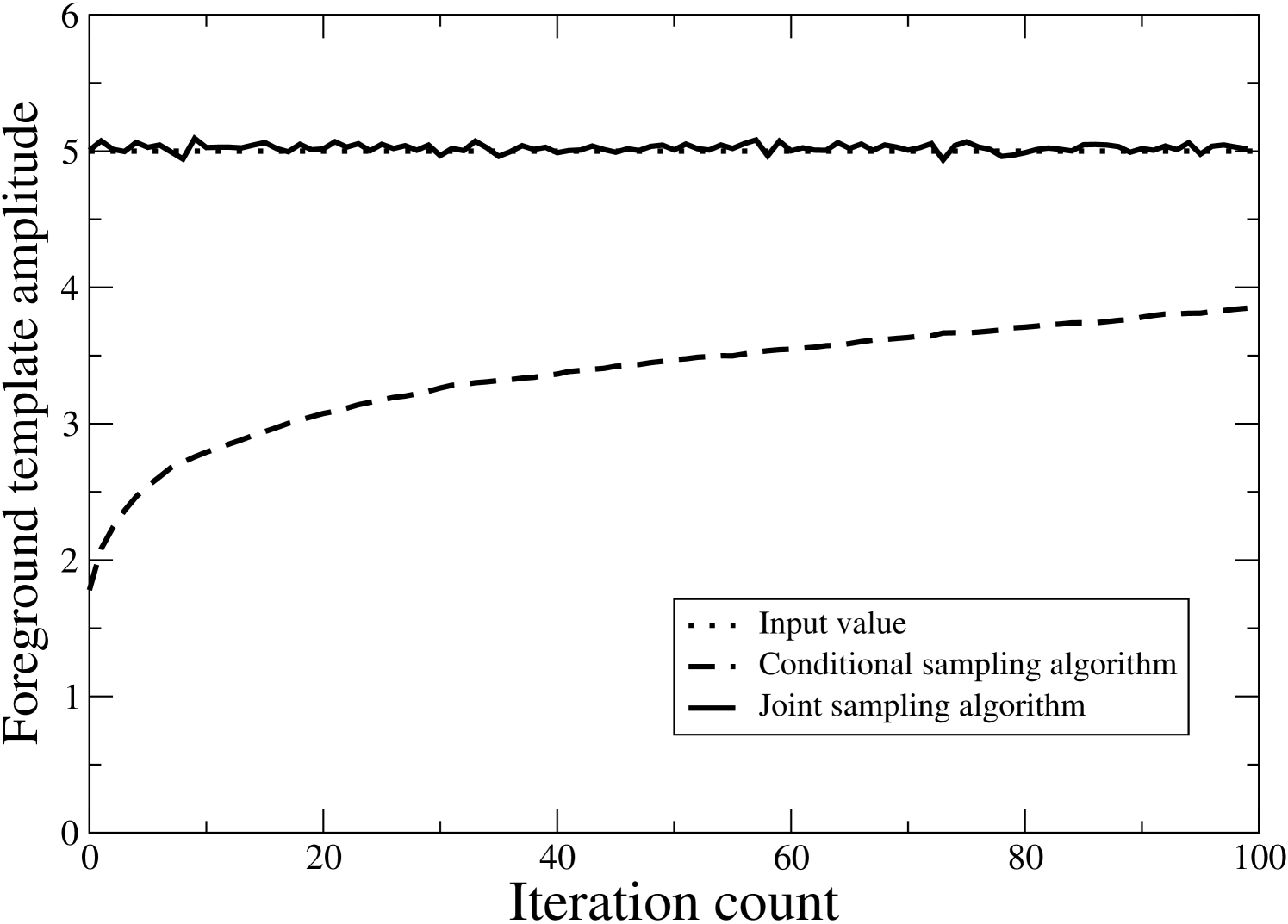
To demonstrate the difference in mixing efficiency between conditional and joint amplitude sampling, Figure 1 shows two trace plots for a high signal-to-noise simulation that included a CMB, a monopole, and a foreground template component. While the joint sampler instantaneously moves into the right regime, and subsequently efficiently explores the correct distribution, the conditional sampler converges only very slowly toward the correct value. The associated long Markov chain correlation length makes this approach unfeasible for general problems.

Refer to caption — Figure 1.— Comparison of trace plots generated by the joint (solid curve) and the conditional (dashed curve) template amplitude sampling algorithms for a simulated data set consisting of a CMB sky signal, a monopole component and a synchrotron template component. The true input template amplitude is shown as a horizontal dotted line.

Preconditioning

The performance of the CG algorithm (see Shewchuk (1994) for an outstanding introduction to this method) depends sensitively on the condition number of the coefficient matrix $\mathcal{A}$ , i.e., the ratio of the largest to the smallest eigenvalue. In fact, the algorithm is not guaranteed to converge at all for poorly conditioned matrices, due to increasing round-off errors in cases that require many iterations.

The condition number of the regularized $\mathcal{A}$ matrix is essentially the largest signal-to-noise ratio of any component in the system, which in practice means that of the CMB quadrupole or the template amplitudes. For current and future CMB experiments, such as WMAP and Planck, the integrated signal-to-noise of these large-scale modes is very large. It is therefore absolutely essential to construct an efficient preconditioner, $\mathbf{M}\approx\mathcal{A}$ , to decouple these modes brute-force, $\mathbf{M}^{-1}\mathcal{A}\mathbf{x}=\mathbf{M}^{-1}\mathbf{b}$ , simply in order to achieve basic convergence.

For the $4\times 4$ coupled system described above, we adopt a three-stage preconditioner. First, for the low- $\ell$ CMB components we explicitly compute all elements of $\mathcal{A}$ up to some $\ell_{\textrm{precond}}\sim 20$ –70 (Eriksen et al., 2004b). This low- $\ell$ block is then coupled to the template amplitudes in a symbolic $3\times 3$ preconditioner,

\mathbf{M}_{0}=\left[\begin{array}[]{ccc}\mathbf{S}^{-1}+\mathbf{A}^{t}\mathbf{N}^{-1}\mathbf{A}&\mathbf{A}^{t}\mathbf{N}^{-1}\mathbf{T}&\mathbf{A}^{t}\mathbf{N}^{-1}\mathbf{F}\\ \mathbf{T}^{t}\mathbf{N}^{-1}\mathbf{A}&\mathbf{T}^{t}\mathbf{N}^{-1}\mathbf{T}&\mathbf{T}^{t}\mathbf{N}^{-1}\mathbf{F}\\ \mathbf{F}^{t}\mathbf{N}^{-1}\mathbf{A}&\mathbf{F}^{t}\mathbf{N}^{-1}\mathbf{T}&\mathbf{F}^{t}\mathbf{N}^{-1}\mathbf{F}\end{array}\right].

(23)

The elements in this matrix are computed by transforming each object individually into spherical harmonic space, including modes only up to $\ell_{\textrm{precond}}$ , and then performing the sums explicitly. (Note that the seemingly intuitive proposition of computing the template elements in pixel space, as opposed to in harmonic space, is flawed; unless all elements are properly bandwidth limited, a non-positive definite preconditioning matrix will result.) For examples of such computations, see Eriksen et al. (2004b).

The second part of our preconditioner regularizes the high- $\ell$ CMB components, and consists of the diagonal elements $\mathcal{A}_{\ell m,\ell^{\prime}m^{\prime}}\delta_{\ell\ell^{\prime}}\delta_{mm^{\prime}}$ from $\ell_{\textrm{precond}}+1$ to $\ell_{\textrm{max}}$ (Eriksen et al., 2004b). The third part of our preconditioner covers the single pixel-pixel foreground amplitudes, which have low signal-to-noise ratio, and are preconditioned with the corresponding diagonal elements of $\mathcal{A}$ only, $\mathbf{G}^{t}\mathbf{N}^{-1}\mathbf{G}$ .

For a typical low-resolution WMAP3 application (five frequency channels degraded to $N_{\textrm{side}}=64$ and $3^{\circ}$ FWHM resolution and regularized with $2\mu\textrm{K}$ RMS white noise), we find that including only the diagonal elements in the above matrix can bring the fractional CG residual down to $\sim 10^{-4}$ , while the recommended convergence criterion for single-precision data is $10^{-6}$ . Thus, including the CMB-template cross-terms in the low- $\ell$ CMB preconditioner in Equation 23 is not just a question of performance for the signal-to-noise levels of WMAP; it is required in order to converge at all. The total number of CG iterations is typically $\lesssim 200$ for the same application with the previously described three-level preconditioner. For some further promising ideas on preconditioning for similar systems, see Smith et al. (2007).

Imposing linear constraints

A useful addition to the above formalism is the possibility of imposing linear constraints on one or more of the parameters. For instance, if it is possible to calibrate the absolute offset of one frequency band by external information, for instance using knowledge about the instrument itself, it would be highly beneficial to fix the corresponding monopole value accordingly. Another constraint may be to exclude template amplitude combinations with a given frequency spectrum, in order to disentangle arbitrary offsets at each frequency from the absolute zero-level of a given foreground component.

In the present code, we have implemented an option for imposing linear constraints on the template amplitudes $\mathbf{a}=\{a_{\nu,i}\}$ on the form

\sum_{\nu,i}q^{k}_{\nu,i}a_{\nu,i}=\mathbf{q}^{k}\cdot\mathbf{a}=0,

(24)

where $\mathbf{q}^{k}=\{q^{k}_{\nu,i}\}$ , $k=1,\ldots,N_{\textrm{c}}$ , are constant orthogonality vectors, and $N_{\textrm{c}}$ is the number of simultaneous linear constraints. For example, if we want to obtain a solution with a fixed monopole amplitude at frequency $\nu_{0}$ , we would set $q_{\nu,i}=\delta_{\nu,\nu_{0}}\delta_{i,0}$ .

The total dimension of the template amplitude vector space is $D=MN_{\textrm{band}}$ , $M$ being the number of free templates at each band. Within this space, the constraint vectors $\mathbf{q}$ span an $N_{\textrm{c}}$ -dimensional sub-space $\mathcal{V}$ to which the CG solution must be orthogonal; $\mathbf{a}$ must lie in the complement of $\mathcal{V}$ , denoted $\mathcal{V}^{\textrm{c}}$ .

To achieve this, we construct a projection operator $P:R^{D}\rightarrow\mathcal{V}^{\textrm{c}}$ by standard Gram-Schmidt orthogonalization, which is a $D\times(D-N_{\textrm{c}})$ -dimensional matrix $\mathbf{P}$ . To impose the constraints defined by Equation 24 on the the final CG solution, Equation 22 is rewritten as

\mathbf{P}^{\textrm{t}}\mathcal{A}^{-1}\mathbf{P}\mathbf{P}^{\textrm{t}}{\bf x}=\mathbf{P}^{t}{\bf b},

(25)

which is solved as before. Corresponding elements in the preconditioner are similarly modified in order to maintain computational efficiency.

3.2.2 Spectral parameter sampling

With the amplitude sampling equations for $P(\mathbf{s},a_{\nu,i},b_{j},\mathbf{c}_{k}|C_{\ell},\theta_{k},\mathbf{d})$ in hand, the only missing piece in the Gibbs sampling scheme defined by Equations 16–18, is a spectral parameter sampler for $P(\theta_{k}|\mathbf{s},a_{\nu,i},b_{j},\mathbf{c}_{k},\mathbf{d})$ . In the FGFit code presented by Eriksen et al. (2006), this task was done by Metropolis-Hastings MCMC, a very general technique that can sample from almost any multi-variate distribution. However, it has two disadvantages. First, hundreds of MCMC steps may be required to generate two uncorrelated samples, making the process quite expensive. Second, and even worse for our application, the chains may need to “burn in” at each main Gibbs iteration, because the amplitude parameters have changed since the last iteration. Proper monitoring of these issues is difficult for problems with tens of thousands of pixels with very different signal-to-noise ratios.

Therefore, we have replaced the MCMC sampler with a direct sampler, specifically a standard inversion sampler, in the present version of our codes. While this algorithm is only applicable for univariate problems, it is also quite possibly the best such sampler, as it draws from the exact distribution, and no computation of acceptance probabilities is needed. The algorithm is the following: First, compute the conditional probability density $P(x|\theta)$ , where $x$ is the currently sampled parameter and $\theta$ denotes the set of all other parameters in the model. In our application, $P(x|\theta)$ is the normalized product of the likelihood $\mathcal{L}$ in Equation 14 and any prior we wish to impose. Then compute the corresponding cumulative probability distribution, $F(x|\theta)=\int_{-\infty}^{x}P(y|\theta)dy$ . Next, draw a random number $u$ from the uniform distribution $U[0,1]$ . The desired sample from $P(x|\theta)$ is given by $F(x|\theta)=u$ .

For multivariate problems we use a Gibbs sampling scheme to draw from the joint distribution, and sample each parameter conditionally. For example, if we want to allow free amplitudes ( $c_{\textrm{s}}$ and $c_{\textrm{d}}$ ) and spectral indices ( $\beta_{\textrm{s}}$ and $\beta_{\textrm{d}}$ ) for both synchrotron and thermal dust emission, the full sampling scheme reads

$\displaystyle\{\mathbf{s},\mathbf{c}_{\textrm{s}},\mathbf{c}_{\textrm{s}}\}^{i+1}$	$\displaystyle\leftarrow P(\mathbf{s},\mathbf{c}_{\textrm{s}},\mathbf{c}_{\textrm{s}}\|C_{\ell}^{i},\beta_{\textrm{s}}^{i},\beta_{\textrm{s}}^{i},\mathbf{d})$	(26)
$\displaystyle C_{\ell}^{i+1}$	$\displaystyle\leftarrow P(C_{\ell}\|\mathbf{s}^{i+1})$	(27)
$\displaystyle\beta_{\textrm{s}}^{i+1}$	$\displaystyle\leftarrow P(\beta_{\textrm{s}}\|\mathbf{s}^{i+1},,\mathbf{c}_{\textrm{s}}^{i+1},\mathbf{c}_{\textrm{s}}^{i+1},\beta_{\textrm{d}}^{i},\mathbf{d})$	(28)
$\displaystyle\beta_{\textrm{d}}^{i+1}$	$\displaystyle\leftarrow P(\beta_{\textrm{d}}\|\mathbf{s}^{i+1},,\mathbf{c}_{\textrm{s}}^{i+1},\mathbf{c}_{\textrm{s}}^{i+1},\beta_{\textrm{s}}^{i},\mathbf{d})$	(29)

Note that it can be beneficial to iterate the latter two equations more than once in each main Gibbs loop, in order to reduce the correlations between consequtive samples cheaply. Typically, with two moderately correlated spectral indices we run $\sim 3$ spectral index iterations for each main Gibbs iteration.

While this approach results in quite acceptable mixing properties for reasonably uncorrelated parameters (e.g., synchrotron and dust spectral indices), other and more efficient methods may be required for more complicated problems. Viable alternatives for such situations are, e.g., rejection sampling or even standard Metropolis-Hastings MCMC with proper burn-in monitoring. The details of the particular sampling algorithm are of little importance as long as it can be proved that the method produces samples from the correct conditional distribution.

4. Marginalization, priors and degeneracies

The algorithm described in §3 provides samples from the full joint posterior $P(\mathbf{s},C_{\ell},a_{\nu,i},b_{j},\mathbf{c}_{k},\theta_{k}|\mathbf{d})$ . From these multivariate samples we estimate each parameter individually by marginalizing over all other parameters in the system and reporting, say, the marginal posterior mean and standard deviation.

This is straightforward, but there are subtleties and care is required. Before applying the method to simulated data in §5 and 6, therefore, we discuss marginalization, priors, degeneracies, and high-dimensional probability distributions.

Much of the following deals with the degeneracy between unknown offsets (or monopoles) at each band and the overall zero-level of a foreground component with a free amplitude at each pixel. The same observations apply to any full-sky template with a free amplitude at each band (e.g., the three dipoles). For simplicity we discuss only offsets below. For the same reason, we neglect the antenna-to-thermodynamic temperature conversion factor. When explicit formulae are derived, the simplified and more readable versions are given in the text; full expressions are given in Appendices B and C.

It turns out that the degeneracy between unknown offsets and the foreground zero-level has almost no effect on the CMB component. For the CMB, the relevant quantity is the sum over all foregrounds, not internal degeneracies among different foregrounds. If one cares only about separating the CMB from foregrounds, and not the foregrounds themselves, much of the following can be ignored.

4.1. The offset-amplitude-spectral index degeneracy for a single pixel

Consider a hypothetical experiment that observes a single pixel at 30, 44, 70, and 100 GHz, with RMS noise 10 $\mu\textrm{K}$ in each band. Assume that the signal is a straight power-law parametrized by amplitude $A$ and spectral index $\beta$ , and that the absolute offset of the detectors is known perfectly for the three highest frequencies, but not for the 30 GHz band. The signal model is

T_{\nu}=m\,\delta_{\nu,\nu_{1}}+A\left(\frac{\nu}{\nu_{1}}\right)^{\beta}.

(30)

There are three free parameters in this system, the offset, amplitude, and spectral index, and four measurements. Since the number of constraints exceeds the number of degrees of freedom, it should be possible to estimate all three parameters individually.

We simulated one realization of this model, adopting the model parameters $A=100\,\mu\textrm{K}$ , $\beta=-3$ and $m=0\,\mu\textrm{K}$ , and adding white noise to each band. Our priors are chosen to be uniform over $-300\,\mu\textrm{K}\leq A,m\leq 300\,\mu\textrm{K}$ and $-6\leq\beta\leq 0$ . We compute the joint posterior by a simple $\chi^{2}$ evaluation over a $200\times 200\times 200$ grid, and marginalize by direct integration.

Figure 2 shows the results in terms of one- and two-dimensional marginal posteriors. The true input values are marked by thick crosses in the top panels and by dashed lines in the bottom panels. The posterior means are shown by dotted lines in the bottom panels.

This simple example highlights two problems that will recur in later sections. First, as the top left panel shows, the offset and amplitude are highly degenerate and anti-correlated; one may add an arbitrary offset to the 30 GHz band and subtract it from the foreground amplitude, without affecting the final $\chi^{2}$ . This degeneracy is a crucial issue for CMB component separation. Many foregrounds have power-law spectra, and differential anisotropy experiments (e.g., WMAP) cannot determine absolute offsets. The monopoles of the WMAP temperature sky maps were determined a posteriori based on a co-secant fit to a crude plane-parallel galaxy model (Bennett et al., 2003b; Hinshaw et al., 2007). This approach is prone to severe modelling errors, precisely because of this type of degeneracy.

The second problem is that integration over a highly degenerate joint posterior yields complicated and strongly non-Gaussian marginal posteriors. Obtaining unbiased point estimates from these posteriors is not trivial. Clearly, the posterior mean is not an unbiased estimator. Further, as we will see in the next section, even the posterior maximum is biased in general, unless special care is taken when choosing priors.

4.2. Uniform vs. Jeffreys’ prior

The strong degeneracies found in the previous example can be broken partially by adding more data. Consider a full-sky data set pixelized at HEALPix resolution $N_{\textrm{pix}}=16$ (3072 independent pixels). Reduce the noise to $1\,\mu\textrm{K}$ RMS per pixel. Use the same signal model as before, but with an offset common to all pixels,

T_{\nu}(p)=m\,\delta_{\nu,\nu_{1}}+A(p)\left(\frac{\nu}{\nu_{1}}\right)^{\beta(p)}.

(31)

We adopt the spatially varying synchrotron model of Giardino et al. (2002) as a template for the amplitude and spectral index of the signal component

We simulated a new data set, and computed the marginal monopole posterior by direct integration. This is straightforward because, for a given value of $m$ , the conditional amplitude-spectral index posterior reduces to a product of single-pixel distributions. The integration therefore goes over a sum of $N_{\textrm{pix}}$ two-dimensional grids, rather than a single $2^{N_{\textrm{pix}}}$ grid.

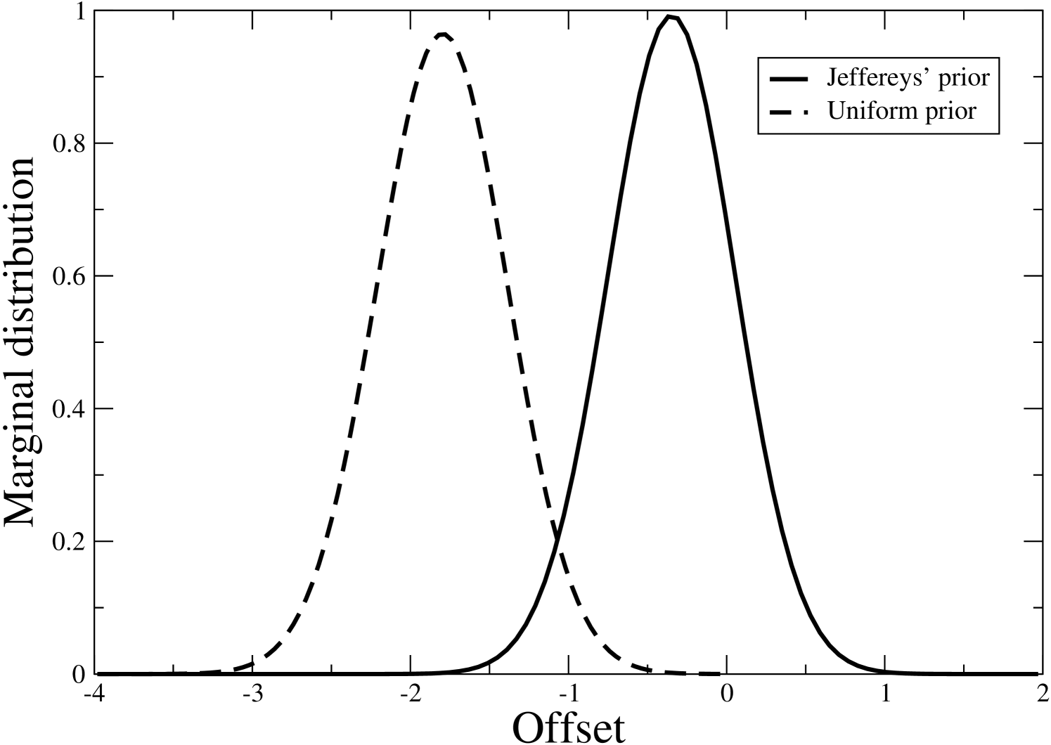
The result is shown as a dashed curve in Figure 3. Two points are noteworthy. First, the marginal distribution is nearly Gaussian, in contrast to the strongly non-Gaussian single-pixel posterior shown in the bottom panel of Figure 2. Thus, the additional data seem to have broken the degeneracy. Second, however, the distribution has a mean and standard deviation of $-1.8\pm 0.4$ , more than 4 $\sigma$ away from zero! Repeated experiments with different noise seeds gave similar results.

This behaviour is a result of the choice of prior. We initially adopted a uniform prior on the offset, the amplitudes and the spectral indices, with little thought to why we should do so. This was a poor choice. Jeffreys (1961) argued that when nothing is known about a particular parameter, one ought to adopt a prior that does not implicitly prefer a given value over another, relative to the likelihood. This is not in general the uniform prior.

Jeffreys argued that the appropriate ignorance prior is given by the square root of the Fisher information measure,

P_{\textrm{J}}(\theta)\sim\sqrt{F_{\theta\theta}}=\sqrt{-\left<\frac{\partial^{2}\ln\mathcal{L}}{\partial^{2}\theta}\right>},

(32)

where the angle brackets indicate an ensemble average. This prior ensures that no parameter region is preferred based on the parametrization of the likelihood alone; it is therefore a proper ignorance prior (e.g., Box & Tiao, 1992).

The log-likelihood corresponding to the model defined in Equation 30 reads

-2\ln\mathcal{L}=\sum_{\nu}\left(\frac{d_{\nu}-m\delta_{\nu,\nu_{1}}-A\left(\frac{\nu}{\nu_{1}}\right)^{\beta}}{\sigma_{\nu}}\right)^{2}.

(33)

Computing the second derivatives of this expression with respect to $A$ , $m$ , and $\beta$ , we find that the appropriate Jeffreys’ priors for the three parameters are

$\displaystyle P_{\textrm{J}}(A)$	$\displaystyle\sim 1,$	(34)
$\displaystyle P_{\textrm{J}}(m)$	$\displaystyle\sim 1,$	(35)
$\displaystyle P_{\textrm{J}}(\beta)$	$\displaystyle\sim\sqrt{\sum_{\nu}{\left(\frac{1}{\sigma_{\nu}}\left(\frac{\nu}{\nu_{1}}\right)^{\beta}\ln\left(\frac{\nu}{\nu_{1}}\right)\right)^{2}}},$	(36)

respectively. In general, the ignorance prior for any linear parameter in a Gaussian model is uniform because the second derivative of the likelihood is constant. However, for non-linear parameters greater care is warranted.

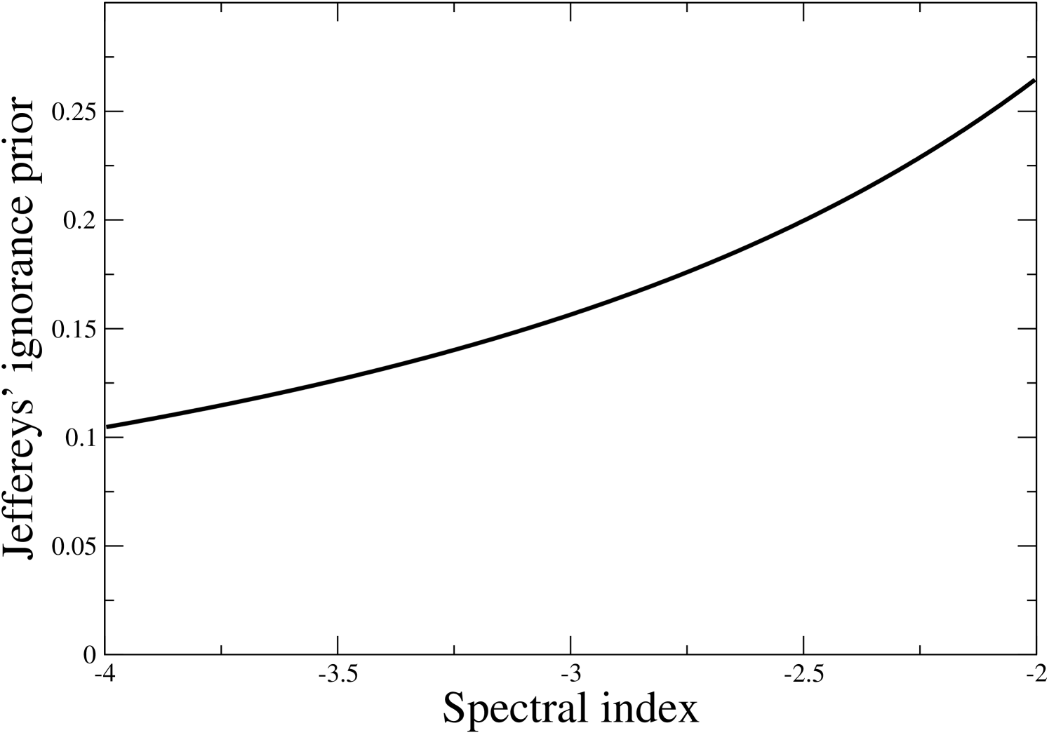
Figure 4 shows Jeffreys’ prior for the spectral index $\beta$ , limited to $-4\leq\beta\leq-2$ . $\beta=-2$ is given about two and half times more weight than $\beta=-4$ . Intuitively, this is necessary because there is an asymmetry between a steep and a shallow spectrum: A steep spectrum means that the signal dies off quickly with frequency, while a shallow spectrum implies that it maintains its strength longer. Thus, there is a larger allowed parameter volume with steep indices than with shallow, leading to an imbalance in terms of marginal probabilities. This parametrization effect is countered by the Jeffreys’ prior.

The solid curve in Figure 3 shows the result of using Jeffreys’ prior instead of a uniform prior. Similar behaviour is observed independent of noise realization. The conclusion is clear: a proper ignorance prior leads to unbiased estimates, while a naive uniform prior leads to biased estimates.

In addition to this basic ignorance prior, it may be beneficial to adopt physical priors, based on knowledge from other experiments. For example, if one had reason to expect that the dominant signal in a given data set were Galactic synchrotron emission, a reasonable prior could be $\beta=-3.0\pm 0.3$ , based on low frequency measurements. The physical prior is multiplied by the ignorance prior, taking account of both effects. In the rest of the paper, when we say that a Gaussian prior is adopted for the spectral indices, we mean a product of a Gaussian and Jeffreys’ prior.

4.3. Marginalization over high-dimensional and degenerate posteriors

The previous section shows that given sufficient data and an appropriate prior, the marginal posterior is a good estimator of the target parameter. In this section we investigate what happens when the data are not sufficiently strong to break a degeneracy. We replace the single-channel offset $m$ by a template amplitude $b$ coupled to a fixed free-free template $t_{\textrm{ff}}(p)$ and a spectral index of $\beta_{\textrm{ff}}=-2.15$ ,

T_{\nu}(p)=b\,t_{\textrm{ff}}(p)\left(\frac{\nu}{\nu_{1}}\right)^{-2.15}+A(p)\left(\frac{\nu}{\nu_{1}}\right)^{\beta(p)}.

(37)

Two modifications are made to the simulation. First, the spectral index of the synchrotron component is fixed to $\beta_{\textrm{s}}=-3$ , rather than being spatially varying. Second, a fifth frequency channel is added at 143 GHz. No free-free component is added to the data; the optimal template amplitude value is zero. The question is whether these data are sufficient to distinguish between synchrotron and free-free emission with similar spectral indices of $-3$ and $-2.15$ , respectively.

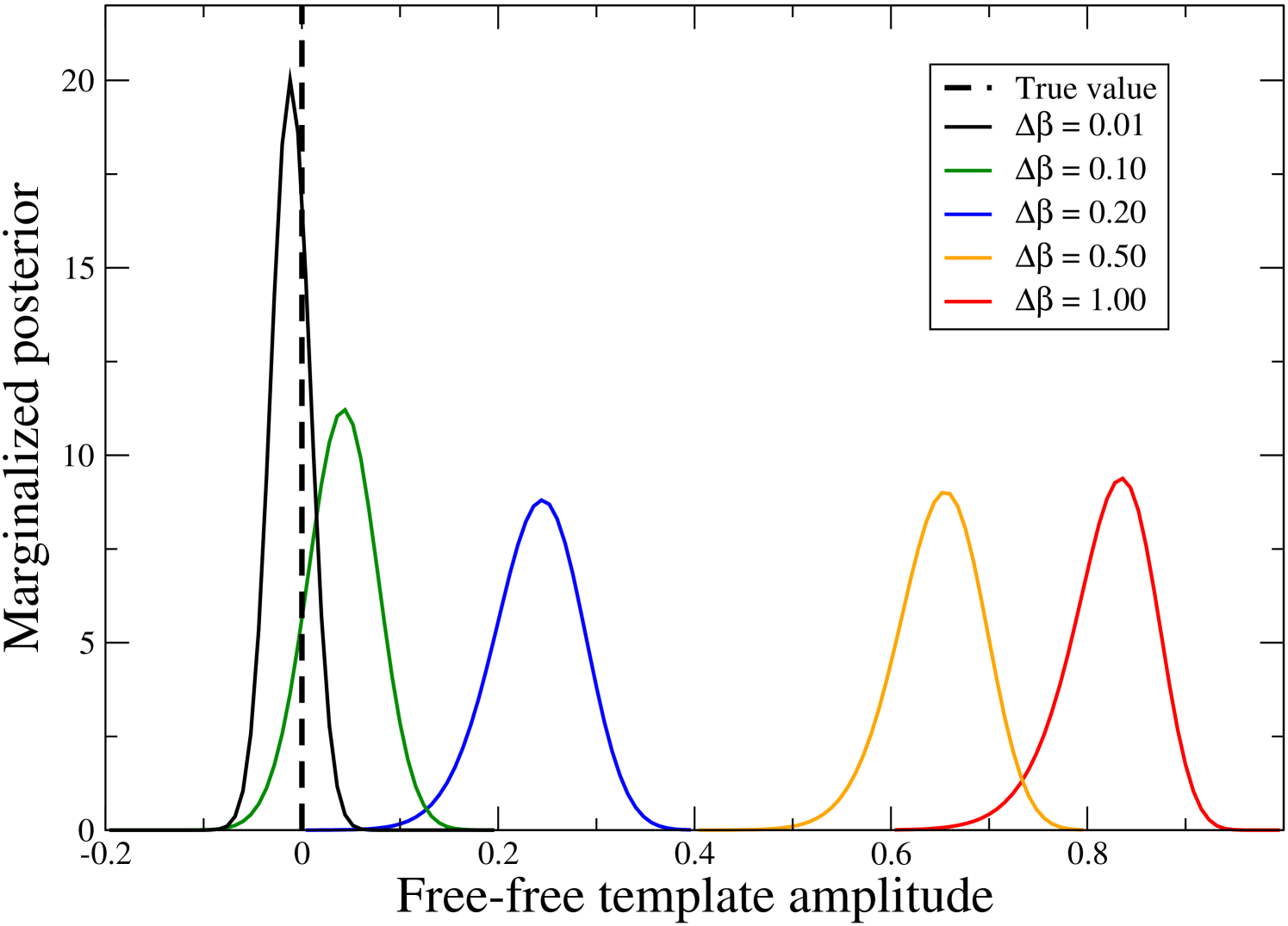
The answer is no. Figure 5 shows the marginal template amplitude posteriors, computed by direct integration as in the previous section. The different curves correspond to different Gaussian priors imposed on the synchrotron spectral index. All are centered on the true value $-3$ , but with different standard deviations $\Delta\beta_{\textrm{s}}$ . With the strong prior of $\Delta\beta_{\textrm{s}}=0.01$ , the amplitude posterior is well-centered near the true value of zero. However, when the prior is gradually relaxed, the marginal posterior widens and drifts away from the true value. The marginal posterior is not a useful estimator for the template amplitude in this case.

This behaviour is explained by the fact that with 3072 independent pixels the contribution of noise to the offset amplitude is insignificant compared to the uncertainty introduced by coupling to the synchrotron component. Moreover, the amplitude and spectral index distributions are similar for the two foreground components. As a result, the joint distribution becomes long, narrow and curved, like that in the top middle panel of Figure 2, The marginal one-dimensional posteriors are dominated by the “boomerang wing” orthogonal to the parameter axis. Similarly, the “wing” parallel to the axis is diluted. Given sufficiently strong degeneracies, the marginal distributions no longer contain the maximum-likelihood point within their, say, $3\sigma$ confidence regions. When the prior is made increasingly tight, however, the wings of the distribution are gradually cut off and the marginal distribution homes in on the true value. Thus, the collection of distributions shown in Figure 5 in some sense visualizes the joint posterior.

This behaviour may be quantified by means of the covariance matrix of the Gaussian amplitude part of the system, defined in Equation 19. A useful quantity describing this matrix is its condition number, the ratio of its largest and smallest eigenvalues. For the particular case discussed above, we find that the condition number is $4\times 10^{6}$ , which, although tractable in terms of numerical precision for double precision numbers¹¹1The absolute limit on the condition number for reliable matrix inversion is $10^{-6}$ for single-precision arithmetic and $10^{-12}$ for double precision. However, in practice one should stay well below these values, in particular for iterative applications since small numerical errors may propagate in an uncontrolled manner., indicates a very strong degeneracy.

4.4. The offset vs. amplitude degeneracy for full-sky data

The final example we consider before turning to realistic simulations is the same as in §4.2, except we allow a free offset for all frequency bands, not just one. (This is characteristic of real experiments, which do not know the absolute zero-point at any frequency.) The model is

T_{\nu}=m_{\nu}+A(p)\left(\frac{\nu}{\nu_{1}}\right)^{\beta(p)}.

(38)

If the spectral index is constant over the sky, $\beta(p)=\beta$ , this is a perfectly degenerate model:

$\displaystyle T_{\nu}$	$\displaystyle=m_{\nu}+A(p)\left(\frac{\nu}{\nu_{1}}\right)^{\beta}$	(39)
	$\displaystyle=(m_{\nu}+\delta m\left(\frac{\nu}{\nu_{1}}\right)^{\beta})+(A(p)-\delta m)\left(\frac{\nu}{\nu_{1}}\right)^{\beta}$	(40)
	$\displaystyle=m^{\prime}_{\nu}+A^{\prime}(p)\left(\frac{\nu}{\nu_{1}}\right)^{\beta}.$	(41)

One can simply add a constant to the foreground amplitude, and subtract a correspondingly scaled value from each offset. It is thus impossible to determine individually the absolute zero-level of foreground component and offsets. To obtain physically relevant results, external information must be imposed.

Spatial variations in the spectral index partially resolve this degeneracy. In the Giardino et al. (2002) synchrotron model the spectral index $\beta_{\textrm{G}}$ varies smoothly on the sky between $-2.5$ and $-3.2$ . The condition number of the foreground amplitude-offset covariance matrix is $2\times 10^{7}$ , and the covariance matrix is no longer singular. A modified index model with ten times smaller fluctuations but the same mean ( $\beta(p)=0.9\left<\beta_{\textrm{G}}\right>+0.1\beta_{\textrm{G}}$ ) increases the condition number by two orders of magnitude, to $2\times 10^{9}$ .

These strong degeneracies lead to the same quantitative behaviour as seen for the marginal free-free template amplitude posterior in the previous section, making it very difficult to estimate both all offsets and the foreground amplitude zero-level individually. In practice, external constraints are required. We have implemented two approaches for dealing with this degeneracy in our code, both based on the projection operator described in §3.2.1.

The first and more direct approach is to assume that the offsets of one or more bands are known a-priori by external information. For instance, if an experiment somehow measured total power, as opposed to differences alone, detailed knowledge about the instrument itself could be used for these purposes. The advantage of this approach is that it is exact, assuming the validity of the prior, and the accuracy of all uncertainties is maintained. It is implemented simply by demanding that $m_{\nu_{0}}=0$ , which requires, in terms of the orthogonality vectors defined in §3.2.1, $q_{\nu,i}=\delta_{\nu,\nu_{0}}\delta_{i,0}$ .

The second approach is based on the observation that the degeneracy between the foreground amplitude and the offsets seen in Equation 41 leads to a very specific frequency distribution of offset amplitudes. Specifically, $m^{\prime}_{\nu}=(m_{\nu}+\delta m(\nu/\nu_{1})^{\beta})$ , where $\delta m$ is an arbitrary constant, but common to all frequency bands. It is therefore possible to require that the set of offsets should not have a frequency spectrum that matches the foreground spectrum.

The corresponding constraint on $m_{\nu}$ may be derived from

\begin{split}\chi^{2}&=\sum_{\nu,pp^{\prime}}\left(m_{\nu}-\delta m\left(\frac{\nu}{\nu_{1}}\right)^{\beta(p)}\right)N_{\nu,pp^{\prime}}^{-1}\\ &\quad\quad\quad\quad\quad\quad\quad\left(m_{\nu}-\delta m\left(\frac{\nu}{\nu_{1}}\right)^{\beta(p^{\prime})}\right).\end{split}

(42)

by first taking the derivative with respect to $\delta m$ , and then enforcing a vanishing foreground component, $\delta m=0$ ,

\sum_{\nu}m_{\nu}\left[\sum_{p,p^{\prime}}N^{-1}_{\nu,pp^{\prime}}\left(\frac{\nu}{\nu_{1}}\right)^{\beta(p^{\prime})}\right]=0

(43)

The expression in brackets says that the offsets should be orthogonal to the mean noise-weighted foreground spectrum.

If the total signal model includes more than one signal component with a free amplitude at each pixel, then these should be included jointly in the above $\chi^{2}$ . A particularly important case is that including both a CMB signal, which has a frequency-independent spectrum, and a proper foreground component. For this case, we have

\begin{split}\chi^{2}&=\sum_{\nu,pp^{\prime}}\left(m_{\nu}-m_{0}-\delta m\left(\frac{\nu}{\nu_{1}}\right)^{\beta(p)}\right)N_{\nu,pp^{\prime}}^{-1}\\ &\quad\quad\quad\quad\quad\quad\quad\left(m_{\nu}-m_{0}-\delta m\left(\frac{\nu}{\nu_{1}}\right)^{\beta(p^{\prime})}\right),\end{split}

(44)

where $m_{0}$ is the additional degree of freedom introduced by the CMB signal. The equivalent constraint on $m_{\nu}$ derived from this expression is notationally more involved (see Appendix C for a full derivation and constraints), but may be written as before in terms a set of orthogonality vectors $q^{i}_{\nu}$ .

While this orthogonality constraint is effective for estimating the absolute zero-level of the foreground component in question, it corresponds to a strong implicit prior that is not likely to be compatible with reality. If there are indeed random offsets at all frequencies, some fractional combination of these offsets will mimic a foreground component. In the above approach, this component is defined to be a foreground signal, rather than an offset. Further, no mixing between the two components is allowed. Thus, the estimated error bars on both the offsets and foreground zero-level will be underestimated.

Recall, however, that this entire discussion concerns the relative contributions to the foreground zero-level and the free offsets, not the CMB signal, which relies on the sum of the two components alone. The fact that the estimated error in the foreground zero-level is under-estimated by a small factor, say, four or five ( $\sigma_{\textrm{est}}\sim 0.5\,\mu\textrm{K}$ vs. $\sigma_{\textrm{true}}\sim 2\,\mu\textrm{K}$ ; see the simulation described in §6), is of no consequence for most applications. Far more important is the fact that this approach provides excellent estimates of both the CMB sky signal and the spectral index distribution, the two quantities where most of the physics lie. This is in sharp contrast to the method employed by the WMAP team, which is based on a co-secant fit to a plane-parallel Galaxy model (Bennett et al., 2003b; Hinshaw et al., 2007). While that specific approach is prone to severe modelling errors because of its lack of detailed foreground modelling, the current approach is internally consistent with respect to all signal components. For more discussion on this issue, see Appendix C, as well as the actual analysis of the 3-yr data presented by Eriksen et al. (2007c). In that analysis, a common offset of $\sim-13\,\mu\textrm{K}$ is detected in all frequency bands, as well as a significant residual dipole in the V-band data.

4.5. Summary

The above discussion may be summarized by the following observations:

•

The marginal mean is a good estimator only for mildly degenerate and non-Gaussian joint distributions. Strongly degenerate models should be avoided, because they are difficult to summarize by simple statistics, and because it takes a prohibitive number of samples to fully explore them.
•

The uniform prior is a proper ignorance prior for Gaussian variables only. In general, Jeffreys’ rule should be used in the absence of informative priors.
•

For experiments with unknown offsets at each frequency band, there is a strong degeneracy between these offsets and the overall zero-level of the foreground amplitudes. This degeneracy should be broken by external or internal priors, if marginal posteriors are to be used as estimators.

5. Code verification

In § 4 we considered simple toy models to develop intuition about the target distributions. We used analytical, brute-force computations to avoid the complexities of real-world computer code. In this section, we turn our attention to Commander, our implementation of the joint foreground-CMB Gibbs sampler described in §3.

Three conditional distributions are involved in this joint Gibbs sampler, namely the CMB power spectrum distribution $P(C_{\ell}|\mathbf{s})$ , the amplitude distribution $P(\mathbf{s},a_{\nu,i},b_{j},\mathbf{c}_{k}|C_{\ell},\theta_{k},\mathbf{d})$ , and the spectral parameter distribution $P(\theta_{k}|\mathbf{s},a_{\nu,i},b_{j},\mathbf{c}_{k},\mathbf{d})$ . In the following three subsections, we test the output from Commander for these three conditional distributions against analytical expressions, at low resolution, to verify both the general sampling algorithms and our specific implementation.

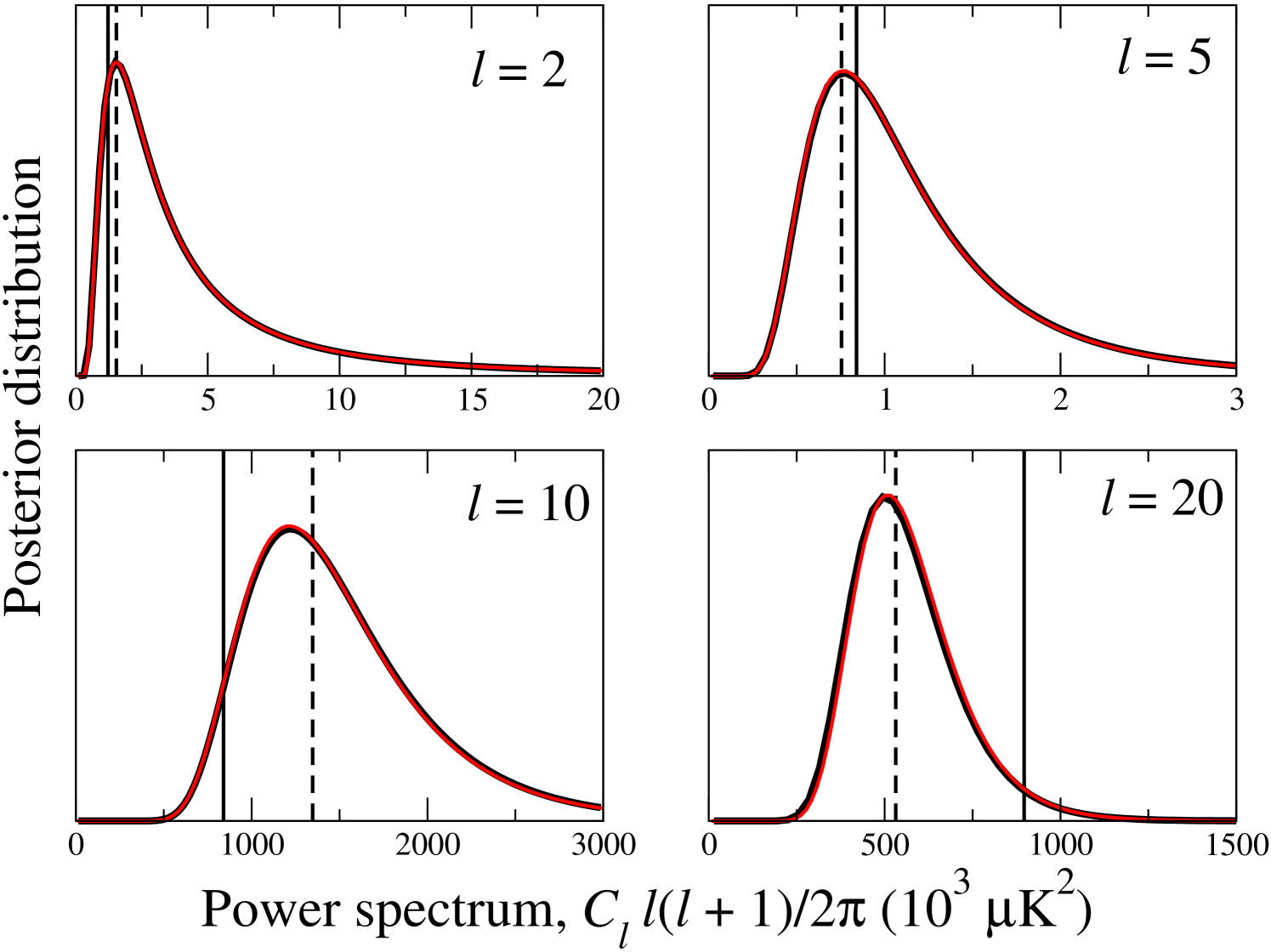
5.1. The CMB power spectrum sampler

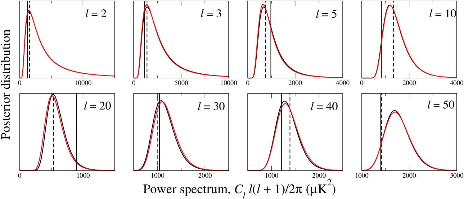
To verify the CMB power spectrum distribution $P(C_{\ell}|\mathbf{s})$ , we construct a low-resolution CMB-only simulation as follows. Draw a random CMB realization from a standard $\Lambda$ CDM power spectrum (Spergel et al., 2007), smooth to $10^{\circ}$ FWHM, and pixelize at $N_{\textrm{side}}=16$ . Add white noise of $1\,\mu\textrm{K}$ RMS to each pixel. Impose the WMAP Kp2 sky cut (Bennett et al., 2003b), without point sources and downgraded to $N_{\textrm{pix}}=16$ , on the data.

We compute slices through the corresponding likelihood by considering each $\ell$ individually, fixing all other multipoles at the input power spectrum, with a brute-force calculation in pixel-space (e.g., Eriksen et al., 2007a), and with Commander. The outputs from the latter are smoothed through Rao-Blackwellization (Chu et al., 2005) to reduce Monte Carlo errors.

Figure 6 shows the results for four multipoles. The theoretical input spectrum is shown by vertical solid lines, and the true realization spectrum by dashed lines. Commander reproduces the CMB power spectrum distributions perfectly.

5.2. The Gaussian amplitude sampler

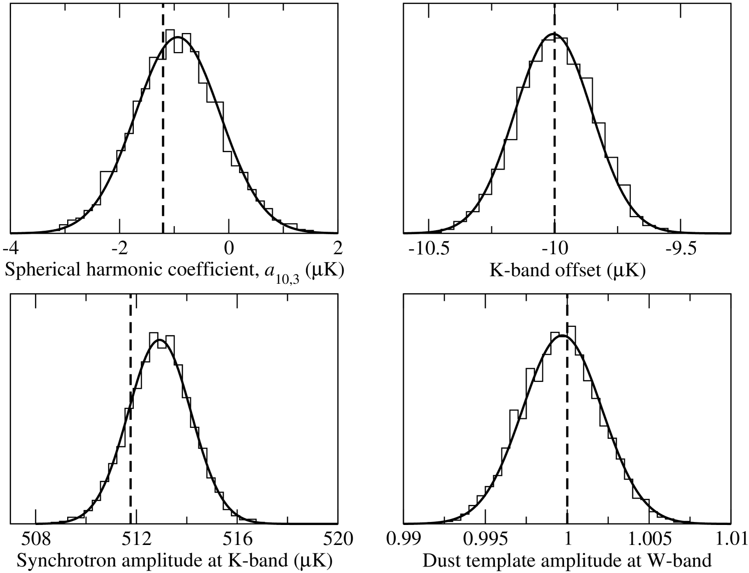
To verify the amplitude distribution $P(\mathbf{s},a_{\nu,i},b_{j},\mathbf{c}_{k}|C_{\ell},\theta_{k},\mathbf{d})$ , we construct a simulation at $N_{\textrm{side}}=8$ (768 independent pixels, angular resolution $20^{\circ}$ FWHM). The CMB realization is the same as in the previous section, appropriately smoothed. Five frequency channels are simulated, corresponding to the five WMAP channels. In addition to the CMB sky signal, $\mathbf{s}$ , we add a synchrotron signal, $\mathbf{c}(p)$ with a spatially varying spectral index, a dust template with an amplitude, $b$ , scaled to unity at W-band, and a $a_{0}=-10\,\mu\textrm{K}$ monopole to the K-band. (See foreground description in Section 6.1 for further details on this model.) Thus, all four types of amplitudes are represented. White noise of $1\,\mu\textrm{K}$ RMS is added to each pixel at each frequency.

We fix the CMB power spectrum and synchrotron spectral index map, and compute the joint Gaussian amplitude distribution both analytically and with Commander. The analytical computation is performed by direct evaluation of the mean $\hat{\mathbf{x}}$ and covariance matrix $\mathcal{A}$ defined by Equations 19 and 20. The marginal variances of each parameter are given by the diagonal elements of $\mathcal{A}$ .

Figure 7 shows the marginal distributions for one parameter of each type. Again, Commander reproduces the exact analytical result perfectly.

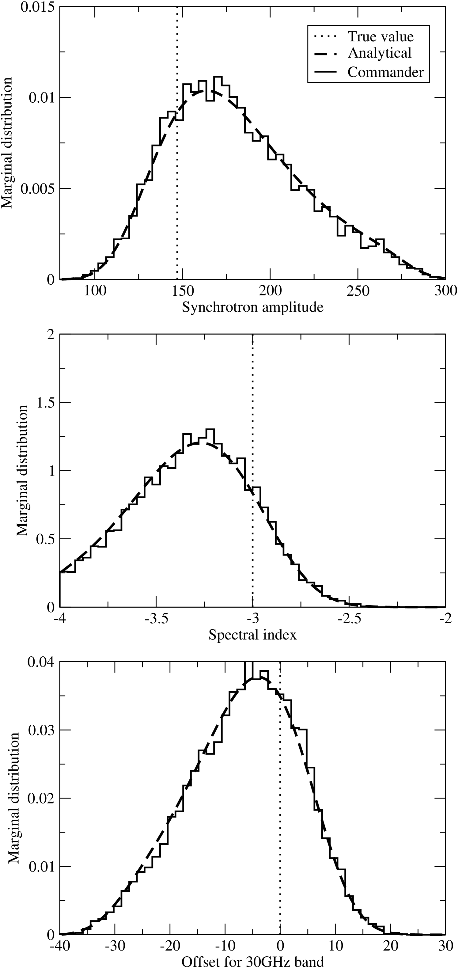
5.3. The spectral index sampler

To verify the spectral index sampler for $P(\theta_{k}|\mathbf{s},a_{\nu,i},b_{j},\mathbf{c}_{k},\mathbf{d})$ , a single-pixel distribution, we simulate a single pixel. The signal model is identical to that in §4.1, comprising a synchrotron component with unknown amplitude and spectral index, plus an unknown offset at the lowest frequency.

We compute the corresponding three-dimensional joint posterior by direct grid evaluation and by Commander. Figure 8 shows the corresponding marginal distributions. Again we find perfect agreement.

All conditional distributions currently implemented in Commander have thus been verified.

6. Application to simulated 3-yr WMAP data

We turn now to a more realistic simulation, with properties corresponding to the 3-yr WMAP data. The simulation has two goals. First, to show that the method can handle data with realistic complexities, and that it is applicable to the current WMAP data and (even more importantly) the up-coming Planck data. Second, to provide the necessary background for understanding the results from the actual 3-yr WMAP analysis presented by Eriksen et al. (2007c).

6.1. Simulation, model and priors

We construct the simulation as follows. Draw a CMB sky realization from the best-fit $\Lambda$ CDM power spectrum presented by Spergel et al. (2007). Convolve with the each of the beams of the ten differencing assemblies of WMAP (Bennett et al., 2003a), pixelized at a HEALPix resolution of $N_{\textrm{side}}=512$ . Add white noise to each map with standard deviation $\sigma(p)=\sigma_{0}/\sqrt{N_{\textrm{obs}}(p)}$ , where $N_{\textrm{pix}}$ is the number of observations at pixel $p$ (provided on Lambda²²2http://lambda.gsfc.nasa.gov together with the actual sky maps).

Downgrade these ten maps to a common resolution of $3^{\circ}$ FWHM and $N_{\textrm{pix}}=64$ , bandlimiting each map at $\ell_{\textrm{max}}=150$ . Create frequency maps by co-adding differencing assembly maps at the same frequency (e.g., Q = (Q1+Q2)/2). Add uniform white noise of $2\,\mu\textrm{K}$ RMS to each frequency map to regularize the noise covariance matrix.

Figure 9 shows the CMB and noise spectra of the co-added V-band data, both at the native resolution of the frequency band (dashed lines) and at the common $3^{\circ}$ FWHM resolution (solid lines). The CMB to regularization noise ratio is unity at $\ell\sim 120$ , and less than 2% at $\ell_{\textrm{max}}=150$ . Both the instrumental and the regularization signal-to-noise ratios are $\gtrsim 500$ at $\ell\leq 50$ , and therefore negligible at these scales compared to cosmic variance.

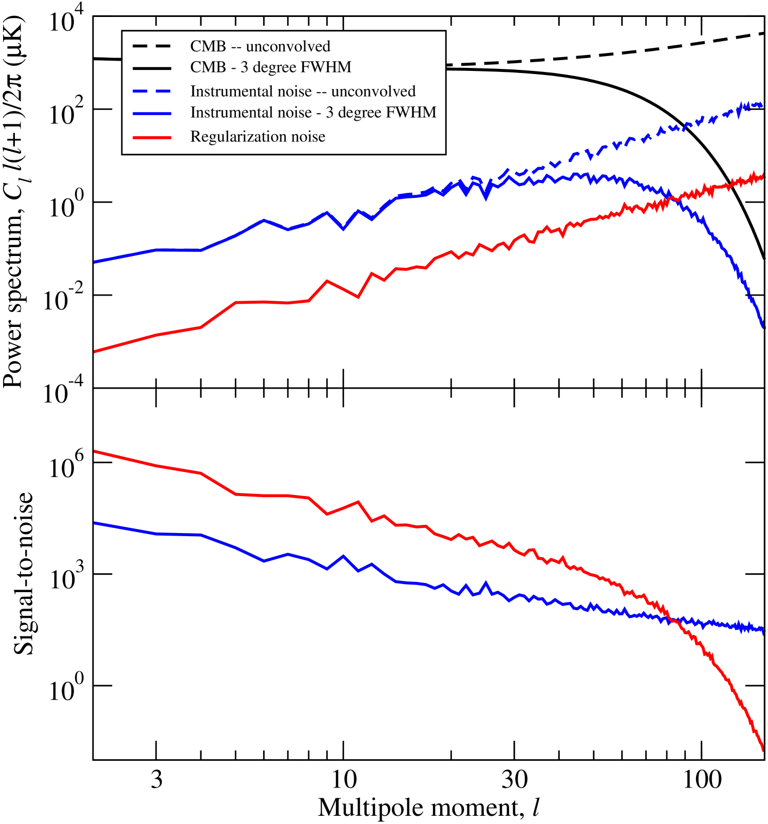
Instrumental noise averaged over the full sky is larger than the regularization noise everywhere below $\ell\lesssim 80$ . In the ecliptic plane, where the instrumental RMS is about a factor of two larger than the full-sky average due to WMAP’s scanning strategy, it dominates below $\ell\lesssim 100$ . The result of this unmodelled noise term is, as we will see later, a somewhat high pixel-by-pixel $\chi^{2}$ in the ecliptic plane. However, since this error term is correlated only on very small scales (the beam size of $3^{\circ}$ FWHM), and we understand its origin and benign behaviour, it does not represent a significant problem for the analysis. With additional years of WMAP observations, and the addition of the Planck data, this noise contribution will be further suppressed. Further, we will consider in the future various approaches for taking this term into account, for instance by computing explicitly the corresponding sparse covariance matrix.

Our foreground model has three components, synchrotron, free-free, and thermal dust emission. For synchrotron emission, where the spectral index is known to vary substantially with position on the sky, we extrapolate the 408 MHz map (Haslam et al., 1982) using a map of the spectral index for each pixel. For the latter we use an updated version of the Giardino et al. (2002) spectral index map that is based on 408 MHz and WMAP 23GHz data, after removing the free-free emission via the WMAP MEM free-freemodel (Bennett et al. 2003b)³³3These models were produced as part of the development of the Planck Sky Model, under the coordination of Planck Working Group 2.. The free-free model is defined by the $H_{\alpha}$ template of Finkbeiner (2003), scaled to 23 GHz assuming an electron temperature of $T_{\textrm{e}}=4000\,\textrm{K}$ and a spatially constant spectral index of $\beta_{\textrm{ff}}=-2.15$ . The dust model is based on model 8 of Finkbeiner et al. (1999), evaluated at 94 GHz and scaled to other frequencies using a single-component modified black-body spectrum with $T_{\textrm{d}}=18.1\,\textrm{K}$ and an emissivity index of $\alpha=2.0$ . Anomalous dust is ignored in this analysis.

Guided by the results of Eriksen et al. (2007c), we add a common offset to all frequencies of $-13\,\mu\textrm{K}$ . No dipole contributions are added to the simulations.

For the power spectrum analysis in §6.4, we analyze the same realization with and without foregrounds, but with the same sky cut. This allows us to distinguish between sky-cut and foreground-induced effects.

We adopt the same parametric signal model as that used by Eriksen et al. (2007c),

\begin{split}T_{\nu}(p)&=s(p)+m^{0}_{\nu}+\sum_{i=1}^{3}m^{i}_{\nu}\left[\hat{\mathbf{e}}_{i}\cdot\hat{\mathbf{n}}(p)\right]+\\ +b&\left[t(p)a(\nu)\left(\frac{\nu}{\nu_{0}^{\textrm{dust}}}\right)^{1.7}\right]+f(p)a(\nu)\left(\frac{\nu}{\nu_{0}}\right)^{\beta(p)}.\end{split}

(45)

The first term is the CMB sky signal. The second and third terms are the monopole $m^{0}$ and three dipole components $m^{i}$ defined by standard Cartesian basis vectors. The fourth term is a dust tracer, based on the FDS template coupled to a fixed spectral index of $\beta_{\textrm{d}}=1.7$ , and a free overall amplitude $b$ . The postulated power-law spectrum does not match the modified black-body spectrum used to create the simulation, and modelling errors are therefore to be expected. The fifth term is a single low-frequency foreground component with a free amplitude $f(p)$ and spectral index $\beta(p)$ at each pixel $p$ . The antenna-to-thermodynamic differential temperature conversion factor is $a(\nu)$ , as always.

In addition to the previously described Jeffreys’ prior, we adopt a prior of $\beta=-3\pm 0.3$ for the low-frequency foreground spectral index, assuming that the foreground signal is synchrotron emission unless the data require otherwise. This is not a particularly strong prior: The free-free spectral index of $\beta_{\textrm{ff}}=-2.15$ is only 2.8 $\sigma$ away from the prior mean, and it does not take a large free-free amplitude to overcome this. For instance, near the galactic plane the standard deviation of the marginal index posterior is $\sim 0.01$ , thirty times smaller than the prior width. At high latitudes, on the other hand, the synchrotron spectral index is for all practical purposes unconstrained. The prior prevents this component from interfering with the CMB signal in regions where its amplitude is low.

We impose the orthogonality constraint discussed in §4.4 to break the degeneracy between the free monopoles and dipoles at each band, and the foreground zero-level and dipole. An important goal in the following is to see whether this approach yields sensible results.

With the simulation, model, and priors defined, we compute the joint and marginal posteriors using the machinery described earlier in the paper. The wall-clock time for generating one single sample is $\sim 50$ s, parallelized over five 2.6 GHz AMD Opteron 2218 processors, one for each frequency band. We generate five chains with 1000 samples each, for a total wall clock time of 14 hr. The total computational cost is 350 CPU hours.

6.2. Burn-in, correlation lengths and convergence

We begin our examination of the results by plotting the output Markov chains as a function of iteration count in Figure 10. Each panel shows the evolution of one parameter, such as the CMB power spectrum coefficient for a single multipole or the dust template amplitude.

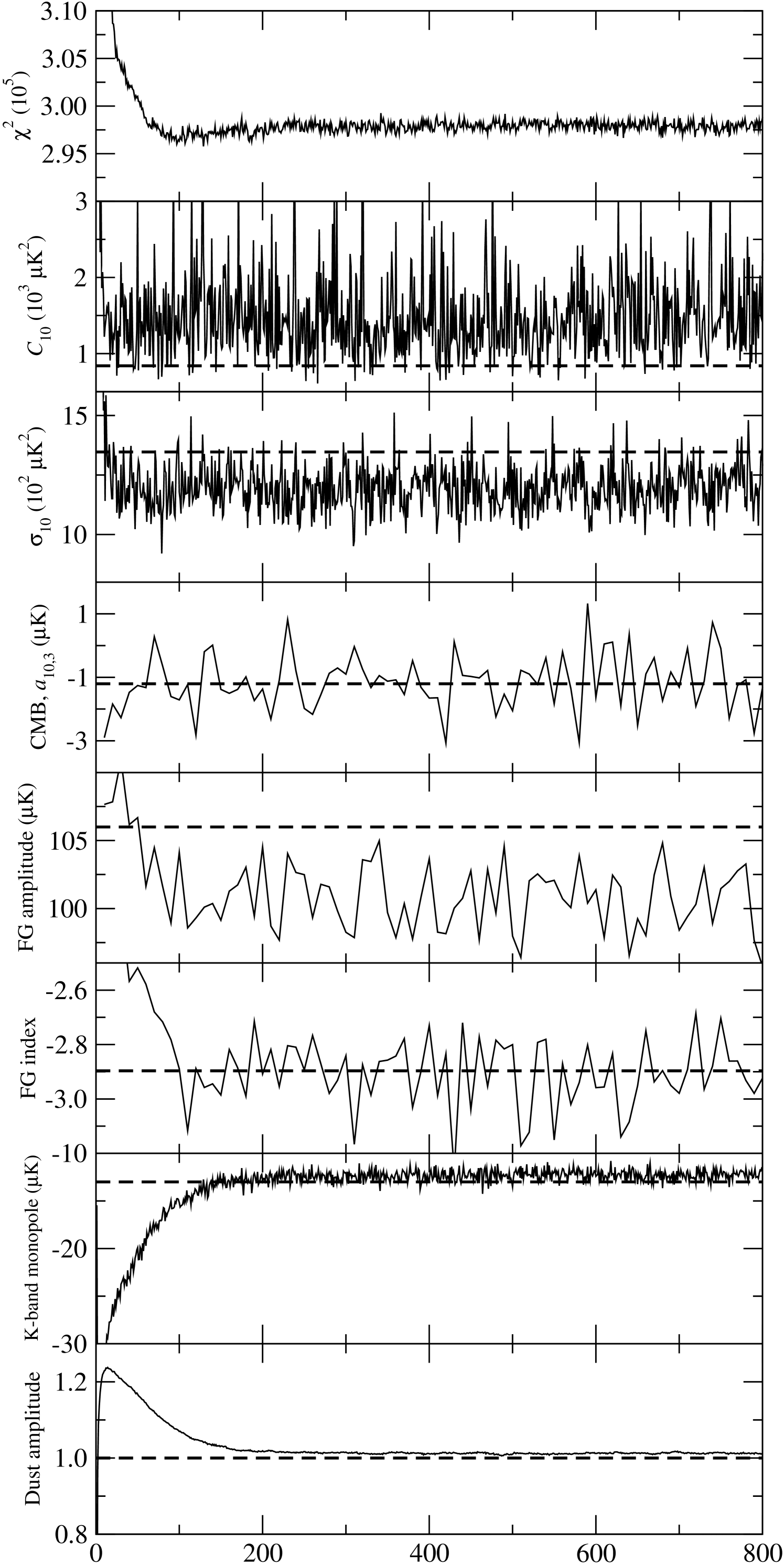
Burn-in is a crucial issue for Markov chain algorithms. The chains were initialized with a random CMB power spectrum over-dispersed relative to the true distribution, and the spectral indices of the low-frequency foreground component were drawn randomly and uniformly between $-4$ and $-2$ . The Gibbs sampler needs some time to converge to the equilibrium distribution; as we see in Figure 10, about 200 iterations are required to reach the equilibrium state.

The last parameters to equilibrate are the global monopole and dust amplitudes, because the uncertainty in these very high signal-to-noise parameters is very small, and only small steps can be made between consecutive Gibbs samples. Moreover, since these are global parameters, they couple to all other parameters.

The $\chi^{2}$ trace plot shows an interesting feature. After reaching a minimum $\chi^{2}$ solution after about 100 iterations, the chain stabilizes at a very slightly higher equilibrium value. This is due to the fact that the full distribution consists not only of the sky signal components, but also the CMB power spectrum. Maximizing the total joint posterior value is therefore a compromise between minimizing the sky signal $\chi^{2}$ and optimizing the CMB power spectrum posterior. At iteration number 100, the CMB component is still burning in, whereas the foreground amplitude, the single most important parameter in terms of $\chi^{2}$ , has already reached its equilibrium. The Markov chain thus overshoots in $\chi^{2}$ minimization until the CMB power spectrum equilibrates.

Correlation length is a second crucial issue for Markov chain algorithms. In general, classic Metropolis-Hastings algorithms have a long correlation length because they propose relatively small modifications at each iteration in order to maintain high acceptance probability. The Gibbs sampler works differently. Because it samples from exact conditional distributions, large jumps are perfectly feasible, at least in the absence of strong conditional correlations. (In the present case there are no such strong correlations.) The CMB power spectrum and CMB sky signal are only weakly correlated in the high signal-to-noise regime, and the foreground spectral index couples only moderately strongly to the foreground amplitude of the same pixel, and weakly to anything else. The result is excellent mixing properties and short correlation lengths.

This translates into a high sampling efficiency and a relatively small number of samples required for convergence. To quantify this, we adopt the widely used Gelman-Rubin $R$ statistic (Gelman & Rubin, 1992), which is the ratio between two variance estimates. If the Markov chains have converged, the two estimates should agree, and their ratio, $R$ , should be close to unity. A typical recommendation is that $R$ should be less than 1.1 to claim convergence, given that the chains were initially over-dispersed, although smaller numbers are clearly better.

Computing this statistic for the five chains above, while discarding the first 200 samples, we find that $R$ is less than 1.01 for the CMB power spectrum up to $\ell\sim 100$ , less than 1.05 for the both the CMB pixel and foreground amplitudes all over the sky, and less than 1.01 for the template amplitudes. Thus, even with such a relatively modest number as 4000 samples, excellent convergence has been reached on all marginal statistics. We return to the question of joint convergence of the CMB spectrum posterior in §6.4.

6.3. Component separation results

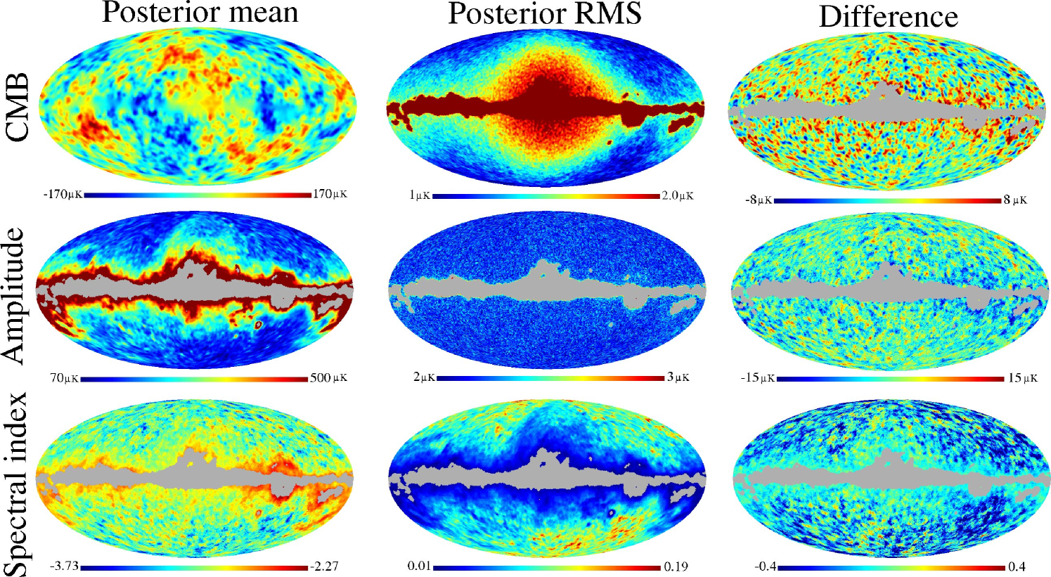
We now turn to the marginal distributions of the estimated signal parameters, and focus first on the signal components. The CMB power spectrum is discussed separately in the next section. The sky map results are summarized in Figure 11 in terms of the marginal posterior means, standard deviations, and differences between the posterior means and the input maps. Table 1 lists the monopole and dipole results. The dust template amplitude posterior mean and standard deviation is $b=1.013\pm 0.002$ .

Considering first the left column in Figure 11, we see that the three sky map reconstructions are visually compelling. No obvious foreground residuals are observed in the CMB map, familiar structures such as the North Galactic Spur and Gum Nebula are seen in the foreground amplitude map, and the spectral index map distinguishes clearly between the known synchrotron and free-free regions.

These visual considerations are quantified in the right column, where the input maps has been subtracted from the posterior means⁴⁴4For the foreground amplitude, the input map was estimated by fitting a single power law to the sum of the synchrotron and free-free components.. We see that the CMB map has residuals at the $\sim 3\,\mu\textrm{K}$ RMS level, with a peak-to-peak amplitude of $\pm 8\,\mu\textrm{K}$ . Little of these residuals is correlated on the sky except for a few patches near the galactic plane. Most of the differences are simply due to instrumental noise.

For the foreground amplitude, more distinct correlated patches are seen, in particular in regions with strong free-free emission. This is due to the fact that a single power law is not a sufficiently good approximation to the sum of the free-free and synchrotron components, relative to the statistical uncertainty.

Table 1Monopole and dipole posterior statistics

	Monopole	Dipole X	Dipole Y	Dipole Z
Band	( $\mu\textrm{K}$ )	( $\mu\textrm{K}$ )	( $\mu\textrm{K}$ )	( $\mu\textrm{K}$ )
K-band	$-12.4\pm 0.5$	$-0.6\pm 0.7$	$-0.4\pm 0.5$	$-0.1\pm 0.1$
Ka-band	$-10.3\pm 0.5$	$-1.2\pm 0.7$	$-0.7\pm 0.5$	$-0.2\pm 0.1$
Q-band	$-10.8\pm 0.5$	$-1.1\pm 0.7$	$-0.7\pm 0.5$	$-0.1\pm 0.1$
V-band	$-12.3\pm 0.5$	$-0.6\pm 0.7$	$-0.6\pm 0.5$	$-0.1\pm 0.1$
W-band	$-12.8\pm 0.5$	$-0.3\pm 0.7$	$-0.2\pm 0.5$	$\,\,\,-0.1\pm 0.1$

Note. — Means and standard deviations of the marginal monopole and dipole posteriors.

Finally, even the the spectral index difference map shows clearly correlated regions, and additionally a negative bias of about $-0.1$ . This bias is primarily due to two effects. First, as reported at the beginning of this section, the dust template amplitude is over-estimated by 1–2%, mainly because of mis-specification of the dust spectrum. As a result, slightly too much signal is subtracted from the higher frequency channels, and this in turn steepens the spectral index of the remaining signal. Second, at high latitudes the data are noise dominated, and the $\beta=-3\pm 0.3$ prior becomes active. Because the true signal has an average of $\sim-2.9$ at high latitudes, a bias of $\sim-0.1$ results.

Comparing the actual difference maps with the estimated errors shown in the middle column of Figure 11, we see that the errors of the CMB and foreground amplitudes are underestimated by a factor of $\sim 1.5$ to 2. (These plots are typically scaled to a dynamical range of $\sim\pm 3\sigma$ . The expected peak-to-peak range in a difference plot is therefore roughly three times the RMS error.) This is due to modelling errors in two forms. First and foremost, we neglected the smoothed instrumental noise in our data model, and this causes a significant unmodelled uncertainty at the smoothing scale. However, being random with zero mean, it does not induce significant structure on larger scales, and it therefore has negligible impact on the scales of cosmological interest ( $\ell\leq 30$ ). Second, the foreground model is simplified compared to the input, as we approximate the sum of two power law components by a single power law, and also assume a simple power-law dust spectrum while the input sky has a modified black-body spectrum. Combined, these effects introduce errors not captured by the estimated statistical uncertainties.

Table 1 lists the posterior mean and standard deviations of the monopole and dipole coefficients. Recall that the input parameters in the two cases were $-13\,\mu\textrm{K}$ and $0\,\mu\textrm{K}$ , respectively. In general, these values are reconstructed reasonably well, although the error estimates are somewhat underestimated for the Ka- and Q-band monopoles. We see that the orthogonality constraint described in §4.4 is quite effective, producing a good estimate of all quantities of interest. On the other hand, it does have the effect of artificially reducing the error bars on the template amplitudes somewhat, and also correlating them. However, misestimation of the monopole error estimates by a few microkelvin is a small price to pay for an absolute estimate of the foreground amplitudes to within a few percent.

The features seen in the CMB RMS map may be understood qualitatively in terms of the above results. First, the most dominating structure is a hot-spot centered on the Galactic plane. This is mainly due to the coupling between the galactic foregrounds and the x-component of the dipole. Because of the large foreground signal in this direction, it is hard to estimate the corresponding dipole component (see Table 1), and this transfers uncertainty from low to high latitudes. Note, however, that this particular component has a very specific correlation structure on the sky, which is taken implicitly into account by the algorithm; this uncertainty does therefore not significantly affect high- $\ell$ modes in the power spectrum, even though it looks visually dominating in a marginal RMS map. Second, the masked Galactic plane has a very high uncertainty, although not infinite; the requirement of isotropy implies that the modes inside this plane is to some extent restricted, at least on large angular scales. Finally, as expected there is a (weaker) correlation between the foreground amplitude and spectral index maps and the CMB RMS map.

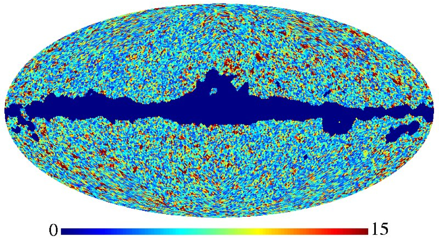
Figure 12 shows the average $\chi^{2}$ computed over the 4000 accepted samples. A value of 15 in this plot corresponds to a model that is excluded at the 99% confidence level. Two points are worth noticing in this plot. First, the ecliptic plane stands out with higher $\chi^{2}$ values. As described above, this is due to the unmodelled, smoothed instrumental noise. At a smoothing scale of $3^{\circ}$ FWHM, this component is not fully negligible for the 3-yr WMAP data relative to the CMB signal, and therefore causes a slight bias at the smallest scales, $\ell\gtrsim 100$ . However, we are mainly interested in $\ell\leq 50$ , and in this range the instrumental signal-to-noise ratio exceeds 100 everywhere. This term does not affect the CMB signal of primary interest.

The actual foreground-induced modelling errors are very small. Indeed, despite the fact that we approximate the sum of two different power laws with a single component, and assume an incorrect dust spectrum, the $\chi^{2}$ distribution is essentially perfect near the ecliptic poles, and the residuals are very small even close to the Galactic plane.

However, the $\chi^{2}$ for the global solution as a whole is somewhat poor, with a reduced $\chi^{2}$ of 1.68. This large value is largely dominated by unmodelled smoothed instrumental noise in the ecliptic plane, as discussed above; when analyzing the same data set at a smoothing scale of $6^{\circ}$ , rather than $3^{\circ}$ , we found a reduced $\chi^{2}\sim 1.1$ . Thus, when using the products from this analysis in subsequent studies (e.g., for cosmological parameter estimation), it is important to include only those scales that are unaffected by the degradation process itself.”

In summary, the overall results are very promising indeed. The CMB sky signal is reconstructed to within a few percent everywhere, as is the foreground amplitude. Further, the spectral indices are accurate to the $\sim 0.1$ level wherever there is a significant signal, and the monopole and dipole coefficients are very close to the true values. Finally, even the reconstructed dust template amplitude is correct to within 2%.

The results are slightly more mixed when it comes to estimation of uncertainties. For components with a relatively large intrinsic uncertainty, such as the CMB sky signal and foreground spectral index, the error estimates are quite reasonable. On the other hand, for parameters with a high intrinsic signal-to-noise ratio, most noticeably the dust template amplitude, the errors are clearly under-estimated because of significant modelling errors. (We note that analysis of simulations with a foreground composition and priors that matches the assumed model yields, as expected from the results shown in Section 5, both point estimates and uncertainties in agreement with expectations.)

The remaining and key issue is what the impact of these residuals and increased uncertainties are on the CMB power spectrum and cosmological parameters at $\ell\leq 30$ . This is the topic of the next section.

6.4. CMB power spectrum and cosmological parameters

We now consider the CMB power spectrum posterior with the goal of understanding the impact of both residual foregrounds and error propagation on the final results. To do so, we consider both the identical simulation described in the previous section and a similar one in terms of instrumental properties and sky coverage, but excluding foregrounds both from the simulated data and the model. Comparing the two against each other allows us to disentangle the effects of foregrounds and sky cut.

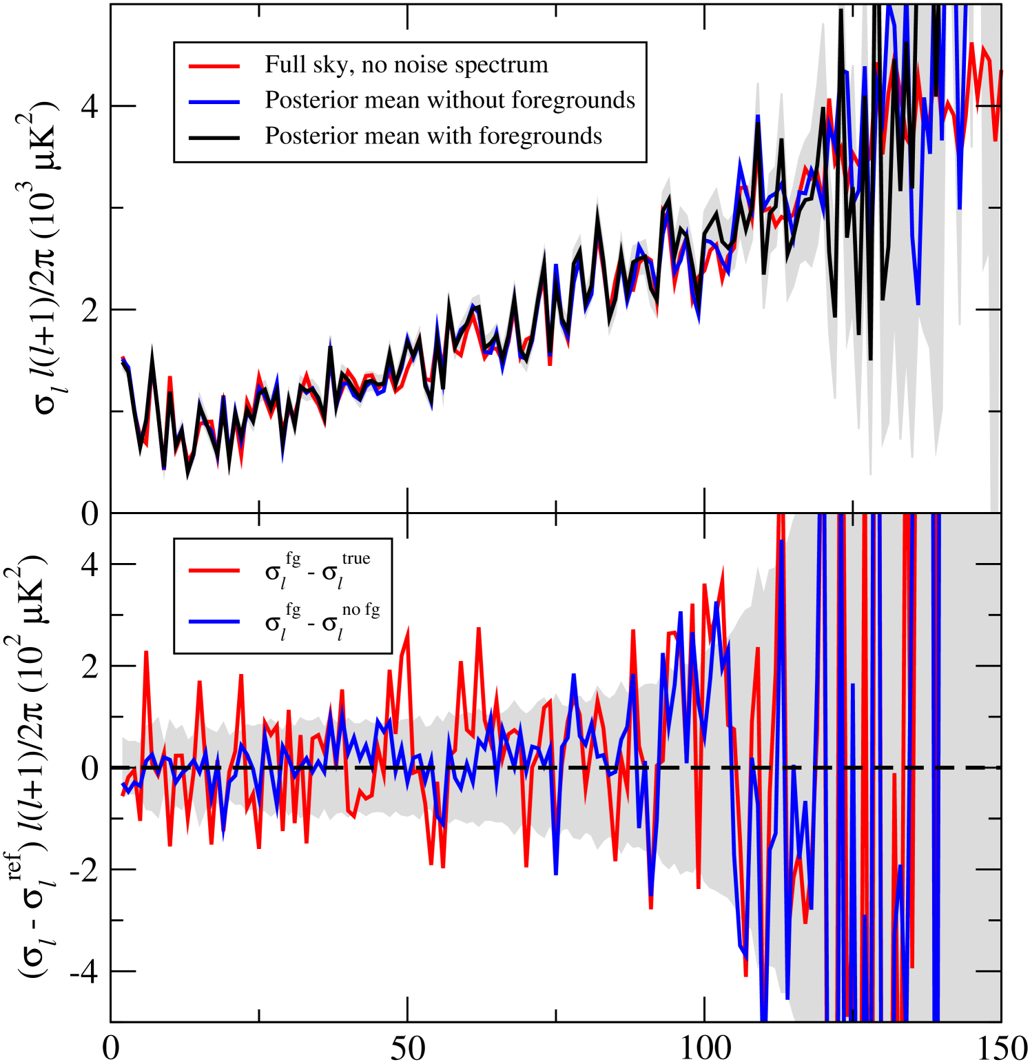
The top panel of Figure 13 shows the posterior mean realization specific spectrum, $\sigma_{\ell}$ , for three different cases. First, the true full-sky spectrum is plotted as a red line. Second, the cut-sky but CMB-only spectrum is shown as blue curve, and finally, the cut-sky and “foreground-contaminated” spectrum is shown as a black curve. The $1\sigma$ confidence region about the latter is marked as a gray region. The bottom panel shows the difference between the foreground-contaminated spectrum and the full-sky spectrum (red), and difference between the two cut-sky spectra (blue).

In terms of absolute differences, we see that the foreground errors (blue curve in Figure 13) are in general less than $50\,\mu\textrm{K}^{2}$ at $\ell\leq 30$ , with a few occasional peaks at $\sim 100\,\mu\textrm{K}^{2}$ , and without any striking biases. Already at this point, we may thus predict that the absolute effect of residual temperature foregrounds on cosmological parameters will be small at large angular scales, when using the component separation method presented in this paper.

Next, we consider the foreground induced uncertainties. First we note that if the total CMB spectrum uncertainty has been properly estimated, then the full-sky difference spectrum (red curve in Figure 13) should be distributed according to the uncertainties indicated by the gray region. Except for some noticeable correlated features around $\ell\approx 50$ , this agreement is quite reasonable. Second, the blue curve shows the differences due to foregrounds alone. This term should thus be described by a corresponding increase in the total uncertainty when including foregrounds in the analysis.

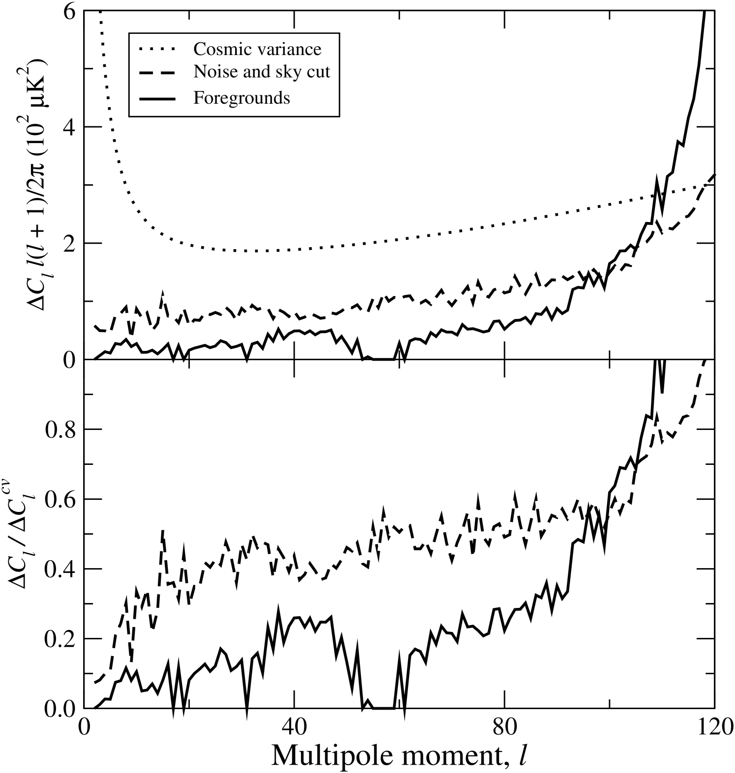
To understand the relative magnitude of these contributions, it is instructive to compute the relative magnitudes of the errors due to cosmic variance, sky cut and instrumental noise, and foregrounds. These can be estimated from quantities ready at hand. First, the standard expression for the cosmic variance is

\textrm{Var}(\textrm{cosmic variance})=\frac{2}{2\ell+1}C_{\ell}^{2}.

(46)

Second, the uncertainty due to the mask and instrumental noise alone is given by the variance of $\sigma_{\ell}^{i}$ ,

\textrm{Var}(\textrm{mask,noise})=\langle(\sigma_{\ell}^{i})^{2}-\langle\sigma_{\ell}^{i}\rangle^{2}\rangle,

(47)

where $\sigma_{\ell}^{i}$ are generated in the analysis without foregrounds. Similarly, the uncertainty due to the combined effect of the mask, instrumental noise, and foregrounds is given by the same expression but computed from the samples that also include foregrounds. To establish an order of magnitude approximation of the foreground-induced uncertainty alone, we assume that the variances add in quadrature,

\textrm{Var}(\textrm{fg})=\textrm{Var}(\textrm{mask,noise,fg})-\textrm{Var}(\textrm{mask,noise})

(48)

This is of course not strictly correct, because the errors in question are quite non-Gaussian, but it is a sufficient approximation for our purposes.

These three functions are shown in the top panel of Figure 14 for the data set described above. In the bottom panel, we show the ratio of the mask and noise error and the foreground error, respectively, to cosmic variance. First we note that the foreground error is always smaller than the mask and noise induced error, except at the very highest $\ell$ ’s, where the estimates are anyway not reliable. However, at $\ell\sim 40$ these two are almost comparable in magnitude, both at the 25–50% level of the cosmic variance. Once again assuming that these errors add in quadrature, neglecting a 20% error term implies underestimating the full errors by about 2% ( $\sqrt{1+0.2^{2}}-1=0.02$ ).

At larger angular scales, we see that the foreground uncertainty becomes essentially irrelevant, simply because the cosmic variance dominates completely: At $\ell\leq 30$ , the relative magnitude of this term is seldom more than 10% of the cosmic variance, which translates to a relative under-estimation of the total error by only 0.5%. This implies a somewhat surprising conclusion: Exact foreground error propagation is not important on the very largest scales, below, say, $\ell\leq 30$ , simply because the cosmic variance is so totally dominating. However, the same does not necessarily hold true on smaller scales. At $\ell\approx 40$ , the foreground error increases the total uncertainty by several percent, and this is likely to increase further to smaller scales⁵⁵5The peculiarly low foreground error at $\ell\approx 50$ may be connected with the lack of features in the dust template at these angular scales; we do not believe it is a general feature.. It could constitute a very significant fraction of the total error in the range between $\ell\sim 50$ –200, depending on the spatial foreground power spectrum.

In Figure 15, we plot eight slices through the power spectrum likelihood between $\ell=2$ and 50, for the two cases that exclude (black curves) and include (red curves) foregrounds. In these plots, we see the same behaviour as discussed above: At very low $\ell$ ’s, the widths of the distributions with and without foregrounds are essentially identical. However, at $\ell=40$ the effect of the foreground uncertainties starts to become visible, as the red distribution is noticeably wider than the black distribution. Still, it is also very clear from this figure that the effect of neglecting foreground errors in the temperature spectrum at $\ell\lesssim 50$ in terms of cosmological parameters will be minimal.

To demonstrate this statement, we define a simple two-parameter power spectrum model,

C_{\ell}=q\left(\frac{\ell}{15}\right)^{n}C_{\ell}^{\textrm{in}},

(49)

where $q$ is a free overall amplitude, $n$ is a spectral tilt parameter, and $C_{\ell}^{\textrm{in}}$ is the actual theoretical power spectrum used to generate the simulation. We then map out the corresponding two-dimensional posterior using the Blackwell-Rao estimator (Chu et al., 2005). The analysis is restricted to the range between $\ell=2$ and 30, which is the primary target range for our first WMAP analysis (Eriksen et al., 2007c).

Figure 16 shows the results in terms of two sets of contours. The dashed contours show the results from the analysis excluding foregrounds, and the solid contours show the results including foregrounds. The true value of $(q,n)=(1,0)$ is marked by a cross. The agreement between the two sets of results is excellent.

Two conclusions may be drawn from this exercise. First, the method presented in this paper is fully capable of extracting the valuable cosmological signal from the 3-yr WMAP data at large angular scales in quite realistic simulations, even when using the simplified foreground model described earlier. Second, the increased uncertainty in cosmological parameters due to these foregrounds at $\ell\lesssim 30$ is negligible.

7. Conclusions

We have presented an algorithm for joint component separation and CMB power spectrum estimation. This algorithm is a natural extension of the CMB Gibbs sampler previously developed by Jewell et al. (2004), Wandelt et al. (2004) and Eriksen et al. (2004b), and the foreground sampler described by Eriksen et al. (2006). The basic product from this algorithm is a set of joint samples drawn from the full joint posterior $P(C_{\ell},\mathbf{s},\theta|\mathbf{d})$ , where $C_{\ell}$ is the CMB power spectrum, $\mathbf{s}$ is the CMB sky signal, and $\theta$ denotes the set of all parameters in the foreground model. With this tool, exact marginalization over very general foreground models is feasible, and proper foreground uncertainties may be propagated seamlessly through to the CMB power spectrum and, therefore, to cosmological parameters.

There are some potential pitfalls the user of the method needs to be aware of before applying it to real data. In particular, one has to pay attention to possible degeneracies in the parametric signal model fitted to the data. Such degeneracies are not uncommon in models relevant to CMB foreground analysis. Two specific examples are synchrotron and free-free emission, with spectral indices of $\beta_{\textrm{s}}\sim-3$ and $\beta_{\textrm{ff}}=-2.15$ , respectively, and the degeneracy between unknown offsets at all frequency bands and the foreground zero-level. In order to obtain reliable one-dimensional marginal estimates of each component individually, one must either make sure that the data have sufficient power to resolve the model, or impose priors to break the degeneracies. Fortunately, since only the sum over all foregrounds is relevant to the actual CMB reconstruction, these issues are of little concern to the cosmological interpretation of the data.

The primary target of this work is Planck, scheduled to be launched in late 2008, and which will observe the microwave sky at nine frequencies from 30 to 857 GHz. Combined with the five WMAP frequencies, these fourteen sky maps will constitute an outstanding data set for both cosmological and Galactic studies. Using the methods described in this paper, it will be possible to constrain three or four foreground components pixel-by-pixel, and even more if adopting spatial templates as priors (e.g., the H_α template as a tracer for free-free).

A more immediate application is the analysis of the 3-yr WMAP temperature data, which is presented in a separate Letter by Eriksen et al. (2007c). As demonstrated in the present paper, the method is fully capable of extracting the valuable cosmological signal at large angular scales from this data set, both in terms of the CMB power spectrum and cosmological parameters. Further, a very general foreground model may be constrained to within a few percent in all parameters.

In its present form, the method assumes identical beam responses at each frequency band. This limits its application to the lowest angular resolution of a given data set. However, this is not a fundamental limitation of the method, but only of our current implementation. Specifically, it is straightforward to rewrite the sampling equations presented in §3 to handle the foreground amplitudes in spherical harmonic space, similar to the current treatment of the CMB sky signal. In that case, convolution with individual beams at each frequency poses no problem. An added bonus is that one may then optionally also either estimate or impose a spatial power spectrum on the foregrounds, just as for the CMB component. The implementation of this is left for future work.

Still, as demonstrated in this paper, even with the current implementation we are able to perform a complete Bayesian joint CMB and foreground analysis with the 3-yr WMAP temperature data at $\ell\lesssim 30$ –50. Simple extrapolation with respect to angular resolution and instrumental noise suggests that we will be able to do at least as well for Planck up to $\ell\sim 100$ –200, beyond which other and simpler approaches may be applicable. We will quantify these projections in greater detail in an upcoming publication where we apply the method to state-of-the-art Planck-based simulations. An important part of this work is to quantify the impact of modelling errors.

To conclude, given the recent successes of the Gibbs sampling approach for analyzing both temperature and polarization CMB data, and now also including realistic foreground modelling, we believe that this method, or generalizations thereof, should be the baseline analysis strategy for Planck at large angular scales. We also note that its computational efficiency and unparallelled capabilities for propagating systematic uncertainties is a combination that will prove extremely valuable to future CMB experiments.

We acknowledge use of the HEALPix software (Górski et al., 2005) and analysis package for deriving the results in this paper. We acknowledge use of the Legacy Archive for Microwave Background Data Analysis (LAMBDA). This work was partially performed at the Jet Propulsion Laboratory, California Institute of Technology, under a contract with the National Aeronautics and Space Administration. HKE acknowledges financial support from the Research Council of Norway, and the hospitality of the Center for Long Wavelength Astrophysics at JPL..

Appendix A The template amplitude coupling matrix

In Section 3.2.1 we described the sampling algorithm for the conditional Gaussian distribution $P(\mathbf{s},a_{\nu,i},b_{j},\mathbf{c}_{k}|C_{\ell},\theta_{k},\mathbf{d})$ . This involved calculating the joint mean,

\hat{{\bf x}}=\mathcal{A}\left[\begin{array}[]{c}\sum_{\nu}\mathbf{A}^{t}\mathbf{N}_{\nu}^{-1}\mathbf{d}\\ \mathbf{t}^{t}_{\nu,j}\mathbf{N}_{\nu}^{-1}\mathbf{d}\\ \sum_{\nu}f_{j}(\nu)\mathbf{f}_{j}^{t}\mathbf{N}^{-1}\mathbf{d}\\ \sum_{\nu}\mathbf{g}_{k}(\nu;\theta_{k})\mathbf{N}_{\nu}^{-1}\mathbf{d}\end{array}\right],

(A1)

and multiplying with the inverse covariance matrix,

\mathcal{A}^{-1}=\left[\begin{array}[]{cccc}\mathbf{S}^{-1}+\mathbf{A}^{t}\mathbf{N}^{-1}\mathbf{A}&\mathbf{A}^{t}\mathbf{N}^{-1}\mathbf{T}&\mathbf{A}^{t}\mathbf{N}^{-1}\mathbf{F}&\mathbf{A}^{t}\mathbf{N}^{-1}\mathbf{G}\\ \mathbf{T}^{t}\mathbf{N}^{-1}\mathbf{A}&\mathbf{T}^{t}\mathbf{N}^{-1}\mathbf{T}&\mathbf{T}^{t}\mathbf{N}^{-1}\mathbf{F}&\mathbf{T}^{t}\mathbf{N}^{-1}\mathbf{G}\\ \mathbf{F}^{t}\mathbf{N}^{-1}\mathbf{A}&\mathbf{F}^{t}\mathbf{N}^{-1}\mathbf{T}&\mathbf{F}^{t}\mathbf{N}^{-1}\mathbf{F}&\mathbf{F}^{t}\mathbf{N}^{-1}\mathbf{G}\\ \mathbf{G}^{t}\mathbf{N}^{-1}\mathbf{A}&\mathbf{G}^{t}\mathbf{N}^{-1}\mathbf{T}&\mathbf{G}^{t}\mathbf{N}^{-1}\mathbf{F}&\mathbf{G}^{t}\mathbf{N}^{-1}\mathbf{G}\end{array}\right].

(A2)

We now write each element in this matrix explicitly, for the benefit of readers who want to implement the algorithm themselves. The elements in the first row of blocks are given by,

$\displaystyle\mathbf{S}^{-1}+\mathbf{A}^{t}\mathbf{N}^{-1}\mathbf{A}$	$\displaystyle\equiv\mathbf{S}^{-1}+\sum_{\nu}\mathbf{A}_{\nu}^{t}\mathbf{N}_{\nu}^{-1}\mathbf{A}_{\nu}$	(A3)
$\displaystyle\mathbf{A}^{t}\mathbf{N}^{-1}\mathbf{T}$	$\displaystyle\equiv\mathbf{A}_{\nu}^{t}\mathbf{N}_{\nu}^{-1}\mathbf{t}_{\nu,j}$	(A4)
$\displaystyle\mathbf{A}^{t}\mathbf{N}^{-1}\mathbf{F}$	$\displaystyle\equiv\sum_{\nu}\mathbf{A}_{\nu}^{t}\mathbf{N}_{\nu}^{-1}f_{j}(\nu)\mathbf{f}_{j}$	(A5)
$\displaystyle\mathbf{A}^{t}\mathbf{N}^{-1}\mathbf{G}$	$\displaystyle\equiv\sum_{\nu}\mathbf{A}_{\nu}^{t}\mathbf{N}_{\nu}^{-1}\mathbf{g}_{k}(\nu;\theta_{k})$	(A6)

The upper part of the second row is

$\displaystyle\mathbf{T}^{t}\mathbf{N}^{-1}\mathbf{T}$	$\displaystyle\equiv\mathbf{t}^{t}_{\nu,j}\mathbf{N}^{-1}\mathbf{t}_{\nu,k}$	(A7)
$\displaystyle\mathbf{T}^{t}\mathbf{N}^{-1}\mathbf{F}$	$\displaystyle\equiv\sum_{\nu}\mathbf{t}^{t}_{\nu,j}\mathbf{N}_{\nu}^{-1}f_{k}(\nu)\mathbf{f}_{j}$	(A8)
$\displaystyle\mathbf{T}^{t}\mathbf{N}^{-1}\mathbf{G}$	$\displaystyle\equiv\sum_{\nu}\mathbf{t}^{t}_{\nu,j}\mathbf{N}_{\nu}^{-1}\mathbf{g}_{k}(\nu;\theta_{k}).$	(A9)

Note that in the above, $\mathbf{T}^{T}\mathbf{N}^{-1}\mathbf{T}$ is the block containing the second derivatives of the log density with respect to the amplitudes $(a_{\nu,j},a_{\nu^{\prime},k})$ , but by the assumed independence of noise at different frequency channels, the terms with $\nu\neq\nu^{\prime}$ vanish. The elements of the upper part of the third row are

	$\displaystyle\mathbf{F}^{t}\mathbf{N}^{-1}\mathbf{F}$	$\displaystyle\equiv\sum_{\nu}f_{j}(\nu)\mathbf{f}^{t}_{j}\mathbf{N}_{\nu}^{-1}\mathbf{f}_{k}f_{k}(\nu)$		(A10)
	$\displaystyle\mathbf{F}^{t}\mathbf{N}^{-1}\mathbf{G}$	$\displaystyle\equiv\sum_{\nu}f_{j}(\nu)\mathbf{f}^{t}_{j}\mathbf{N}^{-1}\mathbf{g}_{k}(\nu;\theta_{k}),$		(A11)

and, finally, for the last block on the diagonal we have

\mathbf{G}^{t}\mathbf{N}^{-1}\mathbf{G}=\sum_{\nu}\mathbf{g}^{t}_{j}(\nu;\theta_{j})\mathbf{N}_{\nu}^{-1}\mathbf{g}_{k}(\nu;\theta_{k}).

(A12)

Appendix B Jeffreys’ ignorance prior for a spectral index

In §4.2 it was shown that to obtain unbiased parameter estimates based on marginal statistics for a power-law foreground model, it is necessary to adopt a proper ignorance prior for the spectral index. In this Appendix we derive the full expression for this prior, including noise and the antenna-to-thermodynamic conversion factor, $a(\nu)$ .

The data model is in this case

d_{\nu}=Aa(\nu)\left(\frac{\nu}{\nu_{1}}\right)^{\beta}+n_{\nu},

(B1)

where $n_{\nu}$ is a noise term with variance $\sigma_{\nu}^{2}=\left<n_{\nu}^{2}\right>$ . We assume no noise correlations between frequencies. The log-likelihood then reads

-2\ln\mathcal{L}(\beta)\propto\sum_{\nu}\left(\frac{d_{\nu}-Aa(\nu)(\nu/\nu_{1})^{\beta}}{\sigma_{\nu}^{2}}\right)^{2}.

(B2)

Jeffreys’ ignorance prior is defined by

P_{\textrm{J}}(\beta)\sim\sqrt{F_{\beta\beta}}=\sqrt{-\left<\frac{\partial^{2}\ln\mathcal{L}}{\partial^{2}\beta}\right>},

(B3)

where the averaging brackets denote an ensemble average. We therefore differentiate the log-likelihood twice and find

-2\frac{\partial^{2}\ln\mathcal{L}}{\partial^{2}\beta}=4\sum_{\nu}\frac{1}{\sigma_{\nu}^{2}}\left\{A^{2}a(\nu)^{2}\left(\frac{\nu}{\nu_{1}}\right)^{2\beta}\ln^{2}\left(\frac{\nu}{\nu_{1}}\right)-\left[d_{\nu}-Aa(\nu)\left(\frac{\nu}{\nu_{1}}\right)\right]Aa(\nu)\left(\frac{\nu}{\nu_{1}}\right)^{\beta}\ln^{2}\left(\frac{\nu}{\nu_{1}}\right)\right\}

(B4)

Taking the ensemble average of this expression simply means setting $\left<d_{\nu}\right>=Aa(\nu)(\nu/\nu_{1})^{\beta}$ , and the second term therefore vanishes,

-\left<\frac{\partial^{2}\ln\mathcal{L}}{\partial^{2}\beta}\right>\propto\sum_{\nu}\frac{A^{2}a(\nu)^{2}}{\sigma_{\nu}^{2}}\left(\frac{\nu}{\nu_{1}}\right)^{2\beta}\ln^{2}\left(\frac{\nu}{\nu_{1}}\right),

(B5)

neglecting irrelevant constants. Thus, the full expression for Jeffreys’ ignorance prior for a spectral index $\beta$ reads

P_{\textrm{J}}(\beta)\propto\sqrt{\sum_{\nu}\frac{a(\nu)^{2}}{\sigma_{\nu}^{2}}\left(\frac{\nu}{\nu_{1}}\right)^{2\beta}\ln^{2}\left(\frac{\nu}{\nu_{1}}\right)}

(B6)

Appendix C Template orthogonality constraints

Most of the discussion in §4 concerned the degeneracy between free offsets at each frequency band and the zero-level of an foreground component with a free amplitude at each pixel. If neither is known, it is possible to add an arbitrary constant to all amplitudes, and subtract a correspondingly scaled value from each free offset, essentially without affecting the final $\chi^{2}$ .

To break this degeneracy, two approaches were proposed. First, if external calibration is possible at one or more frequencies, such information should be exploited and conditioned upon. The second approach was to demand that the free offsets do not have frequency component similar to that of the foreground, by effectively fitting out the corresponding spectrum from the offsets.

These issues apply more generally to any fixed template with a free amplitude at all frequency bands. For most typical applications, this includes also three unknown dipole components, in addition to the familiar offset or monopole. In the following, we simply consider a general collection of templates denoted by $\mathbf{T}$ , which is an $N_{\textrm{pix}}\times N_{\textrm{t}}$ matrix consisting of $N_{\textrm{t}}$ templates listed in its columns. Coupled to this, we define a coefficient vector $\mathbf{a}_{\nu}=\{a_{\nu,i}\}$ containing the template amplitudes for each frequency and template. The sky response at frequency $\nu$ is thus given by $\mathbf{T}\mathbf{a}_{\nu}$ .

We now derive the joint orthogonality constraints for $N_{\textrm{t}}$ templates, for a sky model that includes two components with a free amplitude at each pixel, namely a CMB sky signal and a foreground component with a given frequency spectrum. We denote the vectors of free template coefficients for the CMB and foreground terms by $\mathbf{b}$ and $\mathbf{c}$ , respectively, and the foreground spectrum is defined by the $N_{\textrm{pix}}\times N_{\textrm{pix}}$ diagonal matrix $\mathbf{F}_{\nu}$ having entries equal to $g(\nu;\theta)$ on the diagonal. Note that the frequency spectrum of the CMB component is constant, and the corresponding matrix is therefore the identity. It is omitted in the following.

With this notation, the $\chi^{2}$ to be minimized reads

\chi^{2}=\sum_{\nu}\left(\mathbf{a}_{\nu}^{t}\mathbf{T}^{t}-\mathbf{b}^{t}\mathbf{T}^{t}-\mathbf{c}^{t}\mathbf{F}_{\nu}^{t}\mathbf{T}^{t}\right)\mathbf{N}_{\nu}^{-1}\left(\mathbf{T}\mathbf{a}-\mathbf{T}\mathbf{b}-\mathbf{T}\mathbf{F}_{\nu}\mathbf{c}\right)

(C1)

Equating the derivatives of this expression with respect to $\mathbf{b}$ and $\mathbf{c}$ to zero gives

	$\displaystyle\frac{\partial\chi^{2}}{\partial\mathbf{b}}$	$\displaystyle=-2\sum_{\nu}\mathbf{T}^{t}\mathbf{N}_{\nu}^{-1}\left(\mathbf{T}\mathbf{a}-\mathbf{T}\mathbf{b}-\mathbf{T}\mathbf{F}_{\nu}\mathbf{c}\right)=0$		(C2)
	$\displaystyle\frac{\partial\chi^{2}}{\partial\mathbf{c}}$	$\displaystyle=-2\sum_{\nu}\mathbf{F}_{\nu}^{t}\mathbf{T}^{t}\mathbf{N}_{\nu}^{-1}\left(\mathbf{T}\mathbf{a}-\mathbf{T}\mathbf{b}-\mathbf{T}\mathbf{F}_{\nu}\mathbf{c}\right)=0$		(C3)

These two sets of equations provide a general expression for $\mathbf{a}$ as a function of $\mathbf{b}$ and $\mathbf{c}$ , and at this point we have done nothing more than performed a partial change of basis.

We now impose the prior that breaks the degeneracy between the template and the foreground amplitudes, by requiring $\mathbf{c}=0$ . The two above equations then has a unique solution. In particular, $\mathbf{a}$ is given by

\sum_{\nu}(\mathbf{B}_{\nu}-\mathbf{D}\mathbf{C}^{-1}\mathbf{A}_{\nu})\mathbf{a}=0,

(C4)

where we, for notational transparency, have defined four ancillary matrices

$\displaystyle\mathbf{A}_{\nu}$	$\displaystyle=\mathbf{T}^{t}\mathbf{N}_{\nu}^{-1}\mathbf{T}$	(C5)
$\displaystyle\mathbf{B}_{\nu}$	$\displaystyle=\mathbf{F}^{t}\mathbf{T}^{t}\mathbf{N}_{\nu}^{-1}\mathbf{T}$	(C6)
$\displaystyle\mathbf{C}$	$\displaystyle=\sum_{\nu}\mathbf{A}_{\nu}$	(C7)
$\displaystyle\mathbf{D}$	$\displaystyle=\sum_{\nu}\mathbf{B}_{\nu}.$	(C8)

Note that Equation C4 corresponds to $N_{\textrm{t}}$ separate constraints on $\mathbf{a}$ , and, in particular, each row of the matrix in parentheses defines one orthogonality vector $\mathbf{q}_{\nu}$ . These constraints are thus imposed in the CG solver using the same projection operator method that was described in §3.2.1.

However, we once again stress that this approach corresponds to imposing a very strong prior that is not realized in practice: If there are indeed random fluctuations in the unknown offsets, then these will have a component that happens to have a spectrum similar to the foregrounds. This component will in the present approach be interpreted as a foreground signal. Further, the sampler is by this constraint not allowed to explore the joint distribution between the two components. In other words, both the marginal zero-level and offset uncertainties will be under-estimated by this approach. (Note that most other parameters, such as the CMB signal, are very weakly affected by this, because they only depend on the sum of the two components, not each of the two separately.)

That being said, for experiments where this constraint is required (e.g., differential observatories such as WMAP), it is difficult indeed to construct an alternative and more self-consistent approach. For example, the WMAP team adopted a method based on a co-secant fit to a very crude, plane parallel galaxy model. In their case, no uncertainties were quoted at all. This specific issue is considered in further detail in the actual 3-yr WMAP analysis (Eriksen et al., 2007c).

References

Ade et al. (2007) Ade, P., et al. 2007, ApJ, submitted, [arXiv:0705.2359]
Baccigalupi et al. (2001) Baccigalupi, C., Burigana, C., Perrotta, F., De Zotti, G., La Porta, L., Maino, D., Maris, M., & Paladini, R. 2001, A&A, 372, 8
Baccigalupi (2003) Baccigalupi, C. 2003, New Astronomy Review, 47, 1127
Baccigalupi et al. (2004) Baccigalupi, C., Perrotta, F., de Zotti, G., Smoot, G. F., Burigana, C., Maino, D., Bedini, L., & Salerno, E. 2004, MNRAS, 354, 55
Banday et al. (1996) Banday, A. J., Górski, K. M., Bennett, C. L., Hinshaw, G., Kogut, A., & Smoot, G. F. 1996, ApJ, 468, L85
Barreiro et al. (2004) Barreiro, R. B., Hobson, M. P., Banday, A. J., Lasenby, A. N., Stolyarov, V., Vielva, P., & Górski, K. M. 2004, MNRAS, 351, 515
Bennett et al. (2003a) Bennett, C. L. et al. 2003a, ApJS, 148, 1
Bennett et al. (2003b) Bennett, C. L., et al. 2003b, ApJS, 148, 97
Bond et al. (1998) Bond, J. R., Jaffe, A. H., & Knox, L. 1998, Phys. Rev. D, 57, 2117
Bouchet & Gispert (1999) Bouchet, F. R., & Gispert, R. 1999, New Astronomy, 4, 443
Box & Tiao (1992) Box, G. E. P, & Tiao, G. C. 1992, Bayesian Inference in Statistical Analysis, Wiley Classics Library edition, John Wiley and Sons
Brandt et al. (1994) Brandt, W. N., Lawrence, C. R., Readhead, A. C. S., Pakianathan, J. N., & Fiola, T. M. 1994, ApJ, 424, 1
Chu et al. (2005) Chu, M., Eriksen, H. K., Knox, L., Górski, K. M., Jewell, J. B., Larson, D. L., O’Dwyer, I. J., & Wandelt, B. D. 2005, Phys. Rev. D, 71, 103002
Delabrouille et al. (2003) Delabrouille, J., Cardoso, J.-F., & Patanchon, G. 2003, MNRAS, 346, 1089
Dickinson et al. (2003) Dickinson, C., Davies, R. D., & Davis, R. J. 2003, MNRAS, 341, 369
Donzelli et al. (2006) Donzelli, S., et al. 2006, MNRAS, 369, 441
Efstathiou (2004) Efstathiou, G. 2004, MNRAS, 349, 603
Eriksen et al. (2004a) Eriksen, H. K., Banday, A. J., Górski, K. M., & Lilje, P. B. 2004a, ApJ, 612, 633
Eriksen et al. (2004b) Eriksen, H. K., et al. 2004b, ApJS, 155, 227
Eriksen et al. (2006) Eriksen, H. K., et al. 2006, ApJ, 641, 665
Eriksen et al. (2007a) Eriksen, H. K., et al. 2007a, ApJ, 656, 641
Eriksen et al. (2007b) Eriksen, H. K., Huey, G., Banday, A. J., Górski, K. M., Jewell, J. B., O’Dwyer, I. J., & Wandelt, B. D. 2007b, ApJ, 665, L1
Eriksen et al. (2007c) Eriksen, H. K., Dickinson, C., Jewell, J. B., Banday, A. J., Górski, K. M., & Lawrence, C. R. 2007c, ApJ, submitted, [arXiv:0709.1037]
Finkbeiner et al. (1999) Finkbeiner D.P., Davis M., & Schlegel D.J. 1999, ApJ, 524, 867
Finkbeiner (2003) Finkbeiner, D. P. 2003, ApJS, 146, 407
Gelfand & Smith (1990) Gelfand, A. E., & Smith, A. F. M. 1990, J. Am. Stat. Asso., 85, 398
Gelman & Rubin (1992) Gelman, A., & Rubin, D. 1992, Stat. Sci., 7, 457
Giardino et al. (2002) Giardino, G., Banday, A. J., Górski, K. M., Bennett, K., Jonas, J. L., & Tauber, J. 2002, A&A, 387, 82
Górski (1994) Górski, K. M. 1994, ApJ, 430, L85
Górski et al. (1996) Górski, K. M., Banday, A. J., Bennett, C. L., Hinshaw, G., Kogut, A., Smoot, G. F., & Wright, E. L. 1996, ApJ, 464, L11
Górski (1997) Górski, K. M. 1997, Proc. XVIth Moriond Astrophysics Meeting, Microwave Background Anisotropies, Editions Frontieres, Gif-sur-Yvette, p.77, [astro-ph/9701191]
Górski et al. (2005) Górski, K. M., Hivon, E., Banday, A. J., Wandelt, B. D., Hansen, F. K., Reinecke, M., & Bartelmann, M. 2005, ApJ, 622, 759
Haslam et al. (1982) Haslam, C. G. T., Salter, C. J., Stoffel, H., & Wilson, W. 1982, A&AS, 47, 1
Hinshaw et al. (2007) Hinshaw, G., et al. 2007, ApJS, 170, 288
Hivon et al. (2002) Hivon, E., Górski, K. M., Netterfield, C. B., Crill, B. P.,Prunet, S., & Hansen, F. 2002, ApJ, 567, 2
Hobson et al. (1998) Hobson, M. P., Jones, A. W., Lasenby, A. N., & Bouchet, F. R. 1998,MNRAS, 300, 1
Jeffreys (1961) Jeffreys, H. 1961, Theory of probability, third edition, Oxford, Clarendon Press
Jewell et al. (2004) Jewell, J., Levin, S., & Anderson, C. H. 2004, ApJ, 609, 1
Kuo et al. (2007) Kuo, C. L., et al. 2007, ApJ, 664, 687
Larson et al. (2007) Larson, D. L., Eriksen, H. K., Wandelt, B. D., Górski, K. M., Huey, G., Jewell, J. B., & O’Dwyer, I. J. 2007, ApJ, 656, 653
Lewis & Bridle (2002) Lewis, A., & Bridle, S. 2002, Phys. Rev. D, 66, 103511
Liu (2001) Liu, J. S. 2001, Monte Carlo Strategies in Scientific Computing, Springer
Maino et al. (2002) Maino, D., et al. 2002, MNRAS, 334, 53
Maino et al. (2003) Maino, D., Banday, A. J., Baccigalupi, C., Perrotta, F., & Górski, K. M. 2003, MNRAS, 344, 544
Montroy et al. (2006) Montroy, T. E., et al. 2006, ApJ, 647, 813
O’Dwyer et al. (2004) O’Dwyer, I. J., et al. 2004, ApJ, 617, L99
Page et al. (2007) Page, L., et al. 2007, ApJS, 170, 335
Readhead et al. (2004) Readhead, A. C. S., et al. 2004, ApJ, 609, 498
Shewchuk (1994) Shewchuk, J. R. 1994, http://www.cs.cmu.edu/ $\sim$ quake-papers/painless-conjugate-gradient.ps
Sievers et al. (2007) Sievers, J. L., et al. 2007, ApJ, 660, 976
Smith et al. (2007) Smith, K. M., Zahn, O., & Doré, O. 2007, Phys. Rev. D, 76, 043510
Spergel et al. (2007) Spergel, D. N., et al. 2007, ApJS, 170, 377
Stivoli et al. (2006) Stivoli, F., Baccigalupi, C., Maino, D., & Stompor, R. 2006, MNRAS, 372, 615
Stolyarov et al. (2002) Stolyarov, V., Hobson, M. P., Ashdown, M. A. J., & Lasenby, A. N. 2002, MNRAS, 336, 97
Stolyarov et al. (2005) Stolyarov, V., Hobson, M. P., Lasenby, A. N., & Barreiro, R. B. 2005, MNRAS, 357, 145
Szapudi et al. (2001) Szapudi, I., Prunet, S., & Colombi, S. 2001, ApJ, 561, L11
Tegmark & Efstathiou (1996) Tegmark, M., & Efstathiou, G. 1996, MNRAS, 281, 1297
Tegmark et al. (2003) Tegmark, M., de Oliveira-Costa, A., & Hamilton, A. J. 2003, Phys. Rev. D, 68, 123523
Wandelt et al. (2004) Wandelt, B. D., Larson, D. L., & Lakshminarayanan, A. 2004, Phys. Rev. D, 70, 083511
Wright et al. (1994) Wright, E. L., Smoot, G. F., Bennett, C. L., & Lubin, P. M. 1994, ApJ, 436, 443

	$\displaystyle P(\mathbf{s},C_{\ell}\|\mathbf{d})$	$\displaystyle\propto P(\mathbf{d}\|\mathbf{s},C_{\ell})P(\mathbf{s},C_{\ell})$		(2)
		$\displaystyle\propto P(\mathbf{d}\|\mathbf{s},C_{\ell})P(\mathbf{s}\|C_{\ell})P(C_{\ell}),$		(3)