Joint Calibration of Local Volatility Models with Stochastic Interest Rates using Semimartingale Optimal Transport

Benjamin Joseph¹, Grégoire Loeper², and Jan Obłój³ This research has been supported by BNP Paribas Global Markets and the EPSRC Centre for Doctoral Training in Mathematics of Random Systems: Analysis, Modelling and Simulation (EP/S023925/1).

(¹ Mathematical Institute and Christ Church, University of Oxford
benjamin.joseph@maths.ox.ac.uk
² BNP Paribas Global Markets
gregoire.loeper@bnpparibas.com
³ Mathematical Institute and St John’s College, University of Oxford
jan.obloj@maths.ox.ac.uk )

Abstract

We develop and implement a non-parametric method for joint exact calibration of a local volatility model and a correlated stochastic short rate model using semimartingale optimal transport. The method relies on the duality results established in [18] and jointly calibrates the whole equity-rate dynamics. It uses an iterative approach which starts with a parametric model and tries to stay close to it, until a perfect calibration is obtained. We demonstrate the performance of our approach on market data using European SPX options and European cap interest rate options. Finally, we compare the joint calibration approach with the sequential calibration, in which the short rate model is calibrated first and frozen.

1 Introduction

In financial engineering, calibration refers to the process of adjusting the model’s prices to the market prices. It is an essential task for pricing and hedging derivatives, often performed on an intraday basis.

For this purpose, two class of models emerge: the parametric, and the non-parametric ones. A typical example of parametric model is the Heston model. This type of model allows simplified (semi-analytic) pricing, as well as a clear financial interpretation for each of its parameters; however, its calibration capabilities are limited and it may even struggle to calibrate to a number of instruments comparable to the number of parameters. On the other hand, a non parametric model such as the local volatility model allows to match exactly a whole surface of European option prices, at the expense of requiring numerical simulations, and of lack of interpretability. Nevertheless, it is widely used across the industry.

Recently, a novel non-parametric approach to calibration exploiting semimartingale optimal transport (SOT) has been proposed, and applied for local volatility calibration in [11]. It builds on the methodology introduced in [26] and can also be seen as the stochastic extension of the celebrated time-continuous formulation of the classical OT problem by [2]. This approach is very versatile, and was then extended to local-stochastic volatility models in [12], to general path dependent products and constraints in [8], and to the joint calibration problem of SPX and VIX options in [9]. The last paper in particular showcased the ability of this method to obtain an exact calibration which was known to elude standard parametric models (see [10] for a general discussion on optimal transport based calibration). We mention here an earlier work [1], where the authors followed a similar path to calibration, based on a combination of non parametric exact calibration and regularization via entropic penalization.

All financial products exhibit a dependency to interest rates, as they involve future payments, and it is therefore natural to take into account the stochastic dynamics of interest rates in the calibration procedure. OT based calibration has recently been adapted by the authors of the present study to the context of equity products with stochastic interest rates [18]. Different approaches can be used in this task, either opting for a sequential calibration: the interest rates are calibrated (or given) first, and then a hybrid equity/rates model is calibrated to products exhibiting a dependency to both rates and equity dynamics, or, going for a joint calibration where the full covariance process is calibrated at once using rates and equity market prices.

In [18] a general duality result has been given, that covers both approaches. An application to the former case of sequential calibration was then proposed. This problem is naturally less involved numerically than the joint calibration problem.

In this paper, we use the previous duality result to address the joint calibration problem, given prices of European call options on equity and caps on the short rate. The resulting model is driven by a pair of correlated Brownian motions and has for state variables the equity underlying and the short rate. The algorithm is tested against real market data. We also compare the performance of joint calibration against sequential calibration considered in [18].

2 Formulation of Semimartingale Optimal Transport Calibration Problem

Our method offers exact joint calibration of the stock price’s process and the stochastic short rate processes to market prices of, respectively, European options, European calls and caps. We perform a non-parametric calibration of the drift and diffusion coefficients by recasting the calibration problem as a Semimartingale Optimal Transport (SOT) problem with discrete constraints (given by observed market data). Our SOT reformulation can be seen as a projection on to the space of exactly calibrated models: we start with a given reference model and the cost functional which we seek to penalize deviations from that reference. While enjoying the accuracy of exactly calibrating to chosen product prices, the penalization away from the reference model offers several advantages. First, it convexifies the problem giving a unique solution (for a fixed reference). Second, this convexity is known to give regularity to the solution (see [21], [22]). Third, it gives the user some control about choosing a meaningful reference model from which one tries not to depart too much.

We choose as a starting reference model a classic parametric model, calibrated as well as possible to market prices. As we explain below, to help convergence and smoothness, we propose to update iteratively the reference model: In each iteration, the reference model is taken as the output of the previous iteration. The reference model is also used as the starting point of the gradient descent. This ensures that the reference model is chosen if it matches the calibration constraints.

To illustrate the above methodology, we consider the CEV (constant elasticity of variance) model of [6, 7] under which the underlying, $(S_{t})_{t\geqslant 0}$ , follows

\mathop{}\!\mathrm{d}S_{t}=r_{t}S_{t}\mathop{}\!\mathrm{d}t+\sigma(t,S_{t})S_{t}\mathop{}\!\mathrm{d}W^{1}_{t},

(1)

with $\sigma(t,S_{t})=\sigma S_{t}^{\gamma-1}$ , where $\sigma,\gamma\geqslant 0$ are constants. In the sequel, we write $Z_{t}=\log(S_{t})$ and work with the log-price process. The short rate $(r_{t})_{t\geqslant 0}$ , is modelled using the Vasicek model of [27], and follows

\mathop{}\!\mathrm{d}r_{t}=a(b-r_{t})\mathop{}\!\mathrm{d}t+\sigma_{r}\mathop{}\!\mathrm{d}W^{2}_{t},

(2)

with

\mathop{}\!\mathrm{d}\langle W^{1},W^{2}\rangle_{t}=\rho\mathop{}\!\mathrm{d}t.

(3)

The constants $a,b,\sigma_{r}$ are chosen strictly positive, with $a$ the speed of mean reversion, $b$ the mean, and $\sigma_{r}$ the volatility of the short rate.

All the modelling is done under the risk neutral (pricing) measure and the initial market values $S_{0},r_{0}$ are given. We note that our methods extend easily to non-trivial initial distribution of $S_{0},r_{0}$ which could be useful for forward-starting models, or a multi-period calibration. We fix the parameters of our reference model as $(\overline{\sigma},\overline{\sigma}_{r},\overline{\rho},\overline{a},\overline{b})$ and denote

X_{t}=(X^{1}_{t},X^{2}_{t})=(Z_{t},r_{t}).

(4)

The drift coefficient $\overline{\alpha}(t,X_{t})$ and the diffusion coefficient $\overline{\beta}(t,X_{t})=\frac{d\langle X\rangle_{t}}{dt}$ of the process $X$ under the reference model are thus given by:

(\overline{\alpha}(t,X_{t}),\overline{\beta}(t,X_{t}))=\left(\begin{bmatrix}r_{t}-\frac{1}{2}(\exp(Z_{t}))^{2(\overline{\gamma}-1)}\\ \overline{a}\left(\overline{b}-r_{t}\right)\end{bmatrix},\begin{bmatrix}\overline{\sigma}^{2}\exp(Z_{t})^{2(\overline{\gamma}-1)}&\bar{\rho}\bar{\sigma}\bar{\sigma}_{r}\exp(Z_{t})^{\overline{\gamma}-1}\\ \bar{\rho}\bar{\sigma}\bar{\sigma}_{r}\exp(Z_{t})^{\overline{\gamma}-1}&\bar{\sigma}_{r}^{2}\end{bmatrix}\right).

(5)

Note that on the other hand there is no restriction on the parameters of the calibrating model, apart from risk neutrality and finiteness of the cost function. Our cost function being convex, see (8) below, combined with the classical Markovian mimicking arguments, see [13, 4] and [18, Lemma 3.2], imply that with no loss of generality we can restrict our attention to Markovian models where $\alpha,\beta$ are functions of $(t,X_{t})$ . Note that the initial value $X_{0}\in\mathbb{R}^{2}$ is known and hence a potential candidate model is specified simply via a choice of $(\alpha,\beta):[0,T]\times\mathbb{R}^{2}\to\mathbb{R}^{2}\times\mathbb{S}^{2}_{+}$ , where $\mathbb{S}^{2}_{+}$ are positive definite symmetric $2\times 2$ matrices. Risk neutrality implies $\alpha_{1}=r-\frac{1}{2}\beta_{11}$ . Formally, these observations mean that our candidate model is of the following form, where we take probability measures $\mathbb{P}$ from the set of measures such that $\mathbb{E}^{\mathbb{P}}\left[\int_{0}^{T}\!|\alpha(t,X_{t})|+|\beta(t,X_{t})|\,\mathop{}\!\mathrm{d}t\right]<+\infty$ , which we denote as $\mathbb{P}\in{\mathcal{P}}^{1}$ , and we let $W^{\mathbb{P}}$ be a Brownian motion under $\mathbb{P}$ :

\begin{cases}\mathop{}\!\mathrm{d}X_{t}=\alpha(t,X_{t})\mathop{}\!\mathrm{d}t+(\beta(t,X_{t}))^{\frac{1}{2}}\mathop{}\!\mathrm{d}W_{t}^{\mathbb{P}},&0\leqslant t\leqslant T,\\ X_{0}=x_{0}.&\end{cases}

(6)

Further, we impose bounds on the diffusion coefficients:

\delta^{l}_{11}\leqslant\beta_{11}(t,x)\leqslant\delta^{u}_{11}\qquad\delta^{l}_{22}\leqslant\beta_{22}(t,x)\leqslant\delta^{u}_{22},\qquad\text{for all }(t,x)\in[0,T]\times\mathbb{R}^{2}.

This is desirable from the point of numerical stability, as well as being justifiable from the financial modelling point of view. The drift and diffusion then take values in the following admissible (convex) set, which depends on the interest state variable:

\Gamma_{\mathrm{joint}}(r)\coloneqq\left\{(\alpha,\beta)\in\mathbb{R}^{2}\times\mathbb{S}^{2}_{+}\>:\>\alpha_{1}=r-\frac{1}{2}\beta_{11},\>\delta_{11}^{l}\leqslant\beta_{11}\leqslant\delta^{u}_{11},\>\delta^{l}_{22}\leqslant\beta_{22}\leqslant\delta^{u}_{22}\right\}.

(7)

Define $||\cdot||_{\mathrm{Fro}}$ as the Frobenius norm, which is given by $||M||_{\mathrm{Fro}}=\sqrt{\sum_{i,j}M_{i,j}^{2}}$ . We consider the following cost function $F$

F(\alpha,\beta)=\begin{cases}||\alpha-\overline{\alpha}||^{2}_{2}+||\beta-\overline{\beta}||_{\mathrm{Fro}}^{2},&\mathrm{if}\>(\alpha,\beta)\in\Gamma_{\mathrm{joint}},\\ +\infty,&\mathrm{otherwise}.\end{cases}

(8)

For two square matrices $A,B$ , denote the matrix inner product by $A:B=\mathrm{tr}(A^{\intercal}B)$ . The Legendre-Fenchel transform of $F$ (see [25]) with respect to $(\alpha,\beta)$ is defined by

F^{*}(a,b)\coloneqq\sup_{\begin{subarray}{c}\alpha\in\mathbb{R}^{2},\beta\in\mathbb{S}_{+}^{2}\\ \ \delta^{l}_{11}\leqslant\beta_{11}\leqslant\delta^{u}_{11}\\ \delta^{l}_{22}\leqslant\beta_{22}\leqslant\delta^{u}_{22}\end{subarray}}\{\alpha\cdot a+\beta:b-F(\alpha,\beta)\}.

(9)

We consider market data given as prices of $n$ European options on $X$ . Their maturities and payoffs are denoted respectively by $\tau=(\tau_{1},\dots,\tau_{n})\in(0,T)^{n}$ and $G(x)=(G_{1}(x),\dots,G_{n}(x))$ , and for technical reasons we approximate the call payoffs so that $G_{i}:\mathbb{R}^{2}\to\mathbb{R}$ is continuous and bounded for all $i=1,\dots,n$ . The market price of these options are given by $u=(u_{1},\dots,u_{n})$ so given a candidate model $\mathbb{P}\in{\mathcal{P}}^{1}$ , our market constraints are:

\mathbb{E}^{\mathbb{P}}\left[e^{-\int_{0}^{\tau_{i}}\!r_{s}\,\mathop{}\!\mathrm{d}s}G_{i}(X_{\tau_{i}})\right]=u_{i},\quad i=1,\dots,n.

We denote models $\mathbb{P}\in{\mathcal{P}}^{1}$ such that the above constraints are satisfied as $\mathbb{P}\in{\mathcal{P}}^{1}_{\mathrm{loc}}$ . Note that in practice, we will only consider call options on $S$ and caps on interest rates. Given these constraints, we obtain the reference model (5) via a least squares parametric calibration. Specifically, let $\tilde{u}(\overline{\sigma},\overline{\sigma}_{r},\overline{\gamma},\overline{\rho},\overline{a},\overline{b})\in\mathbb{R}^{n}$ denote the prices of the $n$ options attained our model (1)–(3) with parameters $(\overline{\sigma},\overline{\sigma}_{r},\overline{\gamma},\overline{\rho},\overline{a},\overline{b})$ . The reference model is obtained by numerically solving:

\min_{\overline{\sigma},\overline{\sigma}_{r},\overline{\gamma},\overline{\rho},\overline{a},\overline{b}}\frac{1}{n}\sum_{i=1}^{n}\left(\tilde{u}_{i}(\overline{\sigma},\overline{\sigma}_{r},\overline{\gamma},\overline{\rho},\overline{a},\overline{b})-u_{i}\right)^{2}.

(10)

Where the minimisation is taken over $\overline{\sigma},\overline{\sigma}_{r},\overline{a},\overline{b}>0$ and $\overline{\rho}\in[-1,1]$ . To minimise this, we simply compute the price of the options given the parameters $(\overline{\sigma},\overline{\sigma}_{r},\overline{\gamma},\overline{\rho},\overline{a},\overline{b})$ using the Feynman-Kac formula, then numerically compute the gradients with respect to the parameters using a central difference approximation, and then apply the L-BFGS algorithm of [20]. We ran the optimisation algorithm to a first order error of $1\times 10^{-3}$ , which corresponded to an error of implied volatilities less than $10^{-2}$ in the SPX call options, and of $10^{-1}$ in the short rate cap options.

Parameter	Initial Value	Parametrically Calibrated Value	Interpretation
$\overline{\sigma}$	0.4	0.4115	Volatility scaling of the CEV model
$\overline{\gamma}$	0.9	0.9362	Power law in the CEV model
$\overline{\rho}$	-0.2	-0.2037	Instantaneous correlation between short rate and log-stock
$\overline{\sigma}_{r}$	0.03	0.0232	Volatility of the Vasicek model
$\overline{a}$	0.5	0.0156	Speed of mean reversion in the Vasicek model
$\overline{b}$	0.03	0.2852	Mean to which Vasicek model reverts

Table 1: Reference Model Parameters

Now that the reference model is set, we can formulate the SOT-Calibration problem of [18]. We seek to find

\inf_{\mathbb{P}\in{\mathcal{P}}^{1}_{\mathrm{loc}}}\mathbb{E}^{\mathbb{P}}\left[\int_{0}^{T}e^{-\int_{0}^{t}r_{s}\mathop{}\!\mathrm{d}s}F(\alpha(t,X_{t}),\beta(t,X_{t}))\mathop{}\!\mathrm{d}t\right].

This can rephrased in terms of $(\alpha,\beta)$ and the discounted density $\rho$ , i.e., if for $\mathbb{P}\in{\mathcal{P}}^{1}_{\mathrm{loc}}$ that $\tilde{\rho}(t,x)=\mathbb{P}(X_{t}\in dx)$ is the density of $X_{t}$ then $\rho(t,x)=\mathbb{E}^{\mathbb{P}}[e^{-\int_{0}^{t}r_{s}\,\mathop{}\!\mathrm{d}s}\tilde{\rho}(t,X_{t})|\sigma(X_{t})]$ . We formalise this as follows:

Lemma 2.1 (Lemma 3.3 of [18]).

Let $\mathbb{P}\in{\mathcal{P}}^{1}_{loc}$ so that $X$ solves (6). Let $\eta_{t,x}(\cdot)$ be the law of $\int_{0}^{t}r_{s}\,\mathop{}\!\mathrm{d}s$ conditional on $X_{t}=x$ . Define the ‘discounted density’

\rho(t,x)\coloneqq\left(\int_{\mathbb{R}}e^{-y}\eta_{t,x}(\mathrm{d}y)\right)\bar{\rho}(t,x)=D(t,x)\bar{\rho}(t,x),\qquad(t,x)\in[0,T]\times\mathbb{R}^{2}.

(11)

Then ${\rho}$ solves the ‘discounted’ version of the Fokker-Planck equation for $(t,x)\in[0,T]\times\mathbb{R}^{2}$ :

\partial_{t}{\rho}(t,x)+\nabla_{x}\cdot\left(\alpha(t,x){\rho}(t,x)\right)-\frac{1}{2}\nabla_{x}^{2}:\left(\beta(t,x){\rho}(t,x)\right)+r{\rho}(t,x)=0.

(12)

Problem 2.2 (Primal Problem).

V=\inf_{\rho,\alpha,\beta}\int_{0}^{T}\int_{\mathbb{R}^{2}}\!F(\alpha(t,x),\beta(t,x))\rho(t,\mathop{}\!\mathrm{d}x)\mathop{}\!\mathrm{d}t,

(13)

where the infimum is taken over $(\rho,\alpha,\beta)\in C([0,T];\mathcal{M}(\mathbb{R}^{2}))\times L^{1}(\mathop{}\!\mathrm{d}\rho_{t}\mathop{}\!\mathrm{d}t;\mathbb{R}^{2})\times L^{1}(\mathop{}\!\mathrm{d}\rho_{t}\mathop{}\!\mathrm{d}t;\mathbb{S}^{2})$ subject to:

	$\displaystyle\partial_{t}\rho(t,x)+\nabla_{x}(\rho(t,x)\alpha(t,x))-\frac{1}{2}\nabla^{2}_{x}:(\rho(t,x)\beta(t,x))+r\rho(t,x)$	$\displaystyle=0,\quad(t,x)\in[0,T]\times\mathbb{R}^{2},$
	$\displaystyle\int_{\mathbb{R}^{d}}\!G_{i}(x)\rho(\tau_{i},\mathop{}\!\mathrm{d}x)$	$\displaystyle=u_{i},\quad\text{for }i=1,\dots,n,$
	$\displaystyle\rho(0,\cdot)$	$\displaystyle=\delta_{X_{0}}.$

The above Fokker-Planck equation is understood in the sense of distributions. The duality for the above problem was established in [18, Theorem 3.5] and the dual problem is given by:

Theorem 2.3 (Dual Problem).

V=\sup_{\lambda,\varphi}\lambda\cdot u-\varphi^{\lambda}(0,Z_{0},r_{0}),

where the supremum is taken over $\lambda\in\mathbb{R}^{n}$ and $\varphi^{\lambda}$ is the (unique, discontinuous in time) viscosity solution to the HJB equation:

	$\displaystyle\partial_{t}\varphi^{\lambda}+\sup_{\begin{subarray}{c}\alpha_{2}\in\mathbb{R},\beta\in\mathbb{S}^{2}_{+},\\ \delta^{l}_{11}\leqslant\beta_{11}\leqslant\delta^{u}_{11},\\ \delta^{l}_{22}\leqslant\beta_{22}\leqslant\delta^{u}_{22}\end{subarray}}\biggl{\{}$	$\displaystyle\left(r-\frac{1}{2}\beta_{11}\right)\partial_{z}\varphi^{\lambda}+\alpha_{2}\partial_{r}\varphi^{\lambda}+\frac{1}{2}\beta_{11}\partial^{2}_{zz}\varphi^{\lambda}+\frac{1}{2}\beta_{22}\partial^{2}_{rr}\varphi^{\lambda}+\beta_{12}\partial^{2}_{zr}\varphi^{\lambda}$
		$\displaystyle-\|\|\alpha-\overline{\alpha}\|\|^{2}_{2}-\|\|\beta-\overline{\beta}\|\|^{2}_{\mathrm{Fro}}\biggr{\}}-r\varphi^{\lambda}+\sum_{i=1}^{n}\lambda_{i}G_{i}(x)\delta_{\tau_{i}}=0,\qquad\text{for }(t,x)\in[0,T]\times\mathbb{R}^{2},$		(14)

with terminal condition $\varphi^{\lambda}(T,\cdot)=0$ . If $V$ is finite, then the infimum in Problem 2.2 is attained. If the sup is attained for some $\lambda^{*}$ and corresponding $\varphi^{*}$ solving (14), then the optimisers $(\alpha^{*},\beta^{*})$ are given by

(\alpha_{t}^{*},\beta_{t}^{*})=\nabla F^{*}\left(\nabla_{x}\varphi^{*}(t,\cdot),\frac{1}{2}\nabla^{2}_{x}\varphi^{*}(t,\cdot)\right),\qquad\mathop{}\!\mathrm{d}\rho_{t}\mathop{}\!\mathrm{d}t\text{ - almost everywhere.}

(15)

Note that we use the definition of viscosity solution given in [12, 9, 18], which adapts the classical notion of viscosity solutions from [19] to include the jump discontinuities and also includes the terminal condition $\varphi(T,\cdot)=0$ .

3 Solving the Semimartingale Optimal Transport Calibration Problem

3.1 Numerical Solutions for the Dual Problem

Our numerical approach focuses on solving the dual problem. Specifically, we solve the HJB equation (14) by following [18], which is an adaptation of the methods presented in [12] and [9]. We use a discretisation on a uniform $100\times 100$ spatial grid of $[7.6,8.8]\times[0,5]$ for the log-stock and rescaled interest rates, and partition the time interval into days, so that $\mathop{}\!\mathrm{d}t=\frac{1}{365}$ . We discretise the HJB equation using an implicit finite difference method, with central difference approximations for the spatial derivatives. We choose a boundary far away enough such that the boundary conditions have less of an effect on the HJB equation solution, and our boundary conditions are such that the second derivative of $\varphi$ does not change with time between each calibrating option. That is, for all $x$ on the boundary of our computational domain, and for a subsequence of the calibrating option maturity times $(\tau_{i_{k}})_{k=1,\dots,m}$ such that for $k=1,\dots,m$ all $\tau_{i_{k}}$ are distinct, and with $\tau_{i_{0}}=0$ ,

\nabla^{2}_{x}\varphi(t,x)=\nabla^{2}_{x}\varphi(\tau_{i},x),\quad\text{for }t\in(\tau_{i_{k-1}},\tau_{i_{k}}],\>k=1,\dots,m.

(14) is a fully nonlinear parabolic PDE and we use a policy iteration method (see [24]) as in [18] to solve it. In our policy iteration procedure to approximate $\alpha^{*}$ and $\beta^{*}$ , we compute the finite difference approximations of $\nabla\varphi$ and $\nabla^{2}\varphi$ using $\varphi$ from the previous iteration. The $\varphi$ used in the initial iteration is $\varphi$ from the previous time step (that is $\varphi_{\mathrm{init}}(t_{n},\cdot)\coloneqq\varphi(t_{n+1},\cdot)$ ). With this approximated $(\alpha^{*},\beta^{*})$ , we can apply an implicit finite differences method to one step of the HJB equation to obtain the new value of $\varphi$ . This iteration is repeated until some specified tolerance $\varepsilon_{2}$ is reached such that $||\varphi_{\mathrm{old}}(t_{n},\cdot)-\varphi_{\mathrm{new}}(t_{n},\cdot)||_{\infty}<\varepsilon_{2}$ . In comparison to [18], we are now approximating all of the coefficients, so the iteration takes more steps and thus is less efficient at computing $\alpha^{*}$ and $\beta^{*}$ . The jump discontinuities are handled by simply adding $\lambda_{i}G_{i}(x)$ to the $\varphi_{\mathrm{init}}$ when we reach the timestep corresponding to $\tau_{i}$ . Once we have solved the HJB equation at all time steps, we then solve the linearised model pricing PDE (with coefficients $\alpha^{*}$ and $\beta^{*}$ ) via the ADI method to generate the model prices.

Having solved the HJB equation for a fixed $\lambda$ , we turn our attention to solving Problem 2.3 and finding the optimal $\lambda^{*}$ . First, we observe that we can speed up the optimisation routine by providing a formula for the gradients. This formula is obtained in the same way as [9], but with the discounting appearing as a result of the $-r\varphi$ term in the HJB equation and the Feynman-Kac formula.

Lemma 3.1.

Suppose Problem 2.2 is admissible, and define the dual objective function as

L(\lambda)=\lambda\cdot u-\varphi(0,X_{0}).

(16)

Then the gradients of the dual objective function are given by

\partial_{\lambda_{i}}L(\lambda)=u_{i}-\mathbb{E}^{\mathbb{P}}\left[e^{-\int_{0}^{\tau_{i}}\!r_{s}\,\mathop{}\!\mathrm{d}s}G_{i}(X_{\tau_{i}})\right].

(17)

Our initialisation is $\lambda=0$ since if the reference model is already calibrated, then that will immediately return $||\nabla_{\lambda}L(\lambda)||_{\infty}<\varepsilon_{1}$ . Given a guess $\lambda$ , we solve the HJB equation (14). From the solution of (14), we compute the diffusion coefficients $(\alpha^{*}(t,x),\beta^{*}(t,x))$ from (15). For each instrument we compute the model price by solving

\begin{cases}\partial_{t}\psi(t,x)+\alpha^{*}(t,x)\cdot\nabla_{x}\psi(t,x)+\frac{1}{2}\beta^{*}(t,x):\nabla^{2}_{x}\psi(t,x)-r\psi(t,x)=0,&\quad(t,x)\in[0,\mathcal{T})\times\mathbb{R}^{2},\\ \psi(\mathcal{T},x)=\mathcal{G}(x),&\quad x\in\mathbb{R}^{2}.\end{cases}

(18)

We can then compute the gradient $\nabla_{\lambda}L(\lambda)$ corresponding to the difference between the model prices and and market prices, and finally use the L-BFGS algorithm to update $\lambda$ .

Data: Input an initial

\lambda

and market prices

u_{i}

Result: Calibrated model prices, optimal drift and diffusion

1 while $||\nabla_{\lambda}L(\lambda)||_{\infty}>\varepsilon_{1}$ do

/* Solve the HJB equation backwards in time */

2 for $k=N-1,\dots,0$ do

/* Terminal Conditions - adding

\lambda

multiplied by the payoff */

3 if $t_{k+1}=\tau_{i}$ for some $i=1,\dots,n$ then

\varphi_{t_{k+1}}\leftarrow\varphi_{t_{k+1}}+\sum_{i=1}^{n}\lambda_{i}G_{i}\mathbbm{1}_{\{t_{k+1}=\tau_{i}\}}

5 end if

/* Policy iteration to approximate the optimal characteristics */

\varphi^{\mathrm{new}}_{t_{k}}\leftarrow\varphi_{t_{k+1}}

// Approximate using previous time step

6 while $||\varphi^{\mathrm{new}}_{t_{k}}-\varphi^{\mathrm{old}}_{t_{k}}||>\varepsilon_{2}$ do

\varphi^{\mathrm{old}}_{t_{k}}\leftarrow\varphi^{\mathrm{new}}_{t_{k}}

// Store the old value of

\varphi

Approximate

(\alpha^{*},\beta^{*})

from

\varphi^{\mathrm{old}}_{t_{k}}

// Use old values to approximate optimal characteristics

7 Plug

(\alpha^{*},\beta^{*})

into (14) to remove the supremum and solve using one step of an implicit finite difference method, and set the solution to

\varphi^{\mathrm{new}}_{t_{k}}

8 end while

\varphi_{t_{k}}\leftarrow\varphi^{\mathrm{new}}_{t_{k}}

// Save the solution once the

\varphi

has converged to the optimal solution

10 end for

/* Computing the model prices and gradients */

11 Compute the model prices by solving the pricing PDE (18) using the ADI method.

12 Compute the gradients (17).

13 Use the L-BFGS algorithm to update

\lambda

14 end while

Algorithm 1 Policy iteration algorithm.

3.2 Approximating the optimisers in (15)

In the step 9 of Algorithm 1 we have to Approximate $(\alpha^{*},\beta^{*})$ from $\varphi^{\mathrm{old}}_{t_{k}}$ . This is a key step and it needs to be done efficiently. It is possible to derive an analytic formula for $(\alpha^{*},\beta^{*})$ but this proves to have many subcases and to involve solving quartic equations. In consequence, this method is computationally costly. In our numerical experiments it proved far slower than the alternative which we now describe.

[5] provides a numerical scheme to evaluate the Legendre-Fenchel transform in $O(N^{d}\log N)$ time for $N$ discretisation points and $d$ dimensions. We remark as well that [23] provides a faster version in $O(N^{d})$ time, however it is difficult to separate the $\beta$ terms while maintaining positive semi-definiteness. Since (15) requires the evaluation of the spatial derivatives at all points of the grid, we cannot directly apply the methods to fully take advantage of the faster computational speed. However, we use the observation in equation (2.1) of [5], which allows us to decompose the maximisation component-wise, and apply the idea of evaluating the transform on bounded intervals for computational ease.

Lemma 3.2 (Approximating the Optimal Coefficients).

Define $(\alpha^{*},\beta^{*})$ by:

	$\displaystyle\alpha^{*}_{1}(t,z,r)$	$\displaystyle=r-\frac{1}{2}\beta^{*}_{11}(t,z,r),$
	$\displaystyle\alpha^{*}_{2}(t,z,r)$	$\displaystyle=\overline{\alpha}_{2}(t,z,r)+\frac{1}{2}\partial_{r}\varphi(t,z,r),$
	$\displaystyle\beta^{*}_{11}(t,z,r)$	$\displaystyle=\begin{cases}\overline{\beta}_{11}(t,z,r)+\frac{1}{5}(\partial^{2}_{zz}\varphi(t,z,r)-\partial_{z}\varphi(t,z,r)),&\text{ when }\overline{\beta}_{11}+\frac{1}{5}(\partial^{2}_{zz}\varphi-\partial_{z}\varphi)\in[\delta_{11}^{l},\delta_{11}^{u}],\\ \delta_{11}^{l},&\text{ when }\overline{\beta}_{11}+\frac{1}{5}(\partial^{2}_{zz}\varphi-\partial_{z}\varphi)<\delta_{11}^{l},\\ \delta_{11}^{u},&\text{ when }\overline{\beta}_{11}+\frac{1}{5}(\partial^{2}_{zz}\varphi-\partial_{z}\varphi)>\delta_{11}^{u},\end{cases}$
	$\displaystyle\beta_{22}^{*}(t,z,r)$	$\displaystyle=\begin{cases}\overline{\beta}_{22}(t,z,r)+\frac{1}{4}\partial^{2}_{rr}\varphi(t,z,r),&\text{ when }\overline{\beta}_{22}+\frac{1}{4}\partial^{2}_{rr}\varphi\in[\delta_{22}^{l},\delta_{22}^{u}],\\ \delta_{22}^{l},&\text{ when }\overline{\beta}_{22}+\frac{1}{4}\partial^{2}_{rr}\varphi<\delta_{22}^{l},\\ \delta_{22}^{u},&\text{ when }\overline{\beta}_{22}+\frac{1}{4}\partial^{2}_{rr}\varphi>\delta_{22}^{u},\end{cases}$
	$\displaystyle\beta_{12}^{*}(t,z,r)$	$\displaystyle=\begin{cases}\overline{\beta}_{12}(t,z,r)+\frac{1}{4}\partial^{2}_{zr}\varphi(t,z,r),&\text{ when }\overline{\beta}_{12}+\frac{1}{4}\partial^{2}_{zr}\varphi\in\left[-\sqrt{\beta^{}_{11}\beta^{}_{22}},\sqrt{\beta^{}_{11}\beta^{}_{22}}\right],\\ -\sqrt{\beta^{}_{11}\beta^{}_{22}},&\text{ when }\overline{\beta}_{12}+\frac{1}{4}\partial^{2}_{zr}\varphi<-\sqrt{\beta^{}_{11}\beta^{}_{22}},\\ \sqrt{\beta^{}_{11}\beta^{}_{22}},&\text{ when }\overline{\beta}_{12}+\frac{1}{4}\partial^{2}_{zr}\varphi>\sqrt{\beta^{}_{11}\beta^{}_{22}},\end{cases}$

and $\beta_{21}^{*}=\beta_{12}^{*}$ . The matrix $\beta^{*}$ is positive semidefinite and whenever

-\sqrt{\beta_{11}^{*}\beta_{22}^{*}}<\beta_{12}^{*}<\sqrt{\beta_{11}^{*}\beta_{22}^{*}}

(19)

holds, then $(\alpha^{*},\beta^{*})$ are the optimisers in (15).

The proof is given in Appendix B. It proceeds by solving (15) sequentially: we first solve for $\beta_{11}$ and $\beta_{22}$ subject to their bounds. This is easy to do as the expression is quadratic in each variable. We then solve for $\beta_{12}$ and use it to enforce the condition of positive semi-definiteness on the matrix $\beta$ . If (19) holds then the positive semi-definitiveness condition is not binding and the procedure returns the optimizer. Otherwise, we set $\beta_{12}^{*}=\pm\sqrt{\beta_{11}^{*}\beta_{22}^{*}}$ to ensure $\beta^{*}$ is positive semi-definite but this means our approximation may differ from a global search over all positive semi-definite matrices $\beta$ . However, in all of our numerical experiments, (19) in fact holds everywhere so that, in practice, Lemma 3.2 provides the optimisers in (15) but at a fraction of the computational cost involved in solving (15) analytically as a constrained optimization (29).

3.3 Renormalisation and Reference Model Iteration

As in [18], in order to bring the short rate to the same order as the log-stock for finite difference approximation stability reasons, we perform the constant rescaling $r_{t}\mapsto Rr_{t}$ where we choose $R=100$ . In addition, we rescale the calibrating option prices and their payoffs by their vegas computed from their Black-Scholes implied volatility. This not only helps the stability of the numerical method, but also converts pricing errors into implied volatility errors since the vega represents how much the option price will change as the volatility changes by $1\%$ .

If Algorithm 1 is directly applied, then often it will output a model with spiky drift and diffusion surfaces which is undesirable. This is a result of our cost function penalising deviations from a reference model, which results in larger local changes to the surfaces, but with the rest of the overall surface being closer to the reference model. Moreover, instabilities from the $\partial_{xx}\varphi$ and $\partial_{rr}\varphi$ terms in $\beta_{11}$ and $\beta_{22}$ at maturity at the strikes of our options when adding in the jump discontinuities are unavoidable. In addition, sometimes the L-BFGS algorithm will get stuck and unable to progress. To avoid all of this and improve the convergence to our calibrated model, we apply a “reference model iteration” technique as in [9]. That is, once our optimisation routine finishes, we apply an interpolation and smoothing technique to the output model drift and diffusion terms, and then set those terms to our new reference model and re-run the calibration. The final output model is not smoothed since this would no longer be a calibrated model. This not only speeds up convergence, but also decreased sharp peaks that can arise in our calibrated local volatility surfaces otherwise.

4 Numerical Results: Market Data Example

We test our calibration procedure on market data¹¹1Data obtained from a Bloomberg terminal at the Saïd Business school in Oxford on 23/05/2022.. We used the one month LIBOR as a proxy for the short rate, and obtained the implied volatility and prices of the following options:

•

10 calls on the SPX with expiry 19/08/2022,
•

6 caps on the one month LIBOR with notional $10,000,000 and expiry 23/08/2022,
•

10 calls on the SPX with expiry 18/11/2022,
•

6 caps on the one month LIBOR with notional $10,000,000 and expiry 23/11/2022.

We have a total of $n=32$ options with payoff functions $G_{i}(X_{\tau_{i}})=(\exp(X^{1}_{\tau_{i}})-K_{i})^{+}$ for the calls and $G_{i}(X_{\tau_{i}})=N\tau_{i}(X^{2}_{\tau_{i}}-K_{i})^{+}$ for the caps, where $N$ is the notional value.

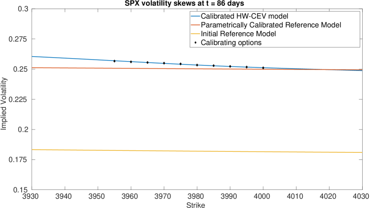
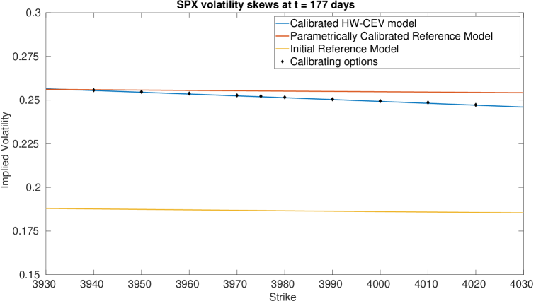
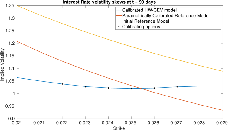
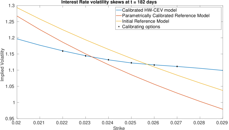
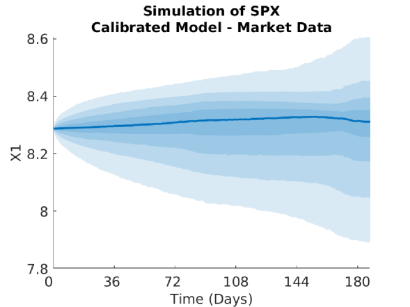
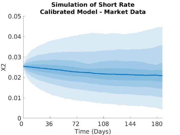
Refer to caption — Figure 1: Implied volatility skews of the SPX calibrating options under the reference model and calibrated HW-CEV model.

We display the optimisation parameters, and the bounds for $\beta_{11}$ and $\beta_{22}$ below. It is difficult to choose the bounds since too relaxed a bound will result in large values for $\beta_{11}$ and $\beta_{22}$ and also result in numerical instabilities for $\beta_{12}$ ; whereas too tight a bound will severely slow down the calibration. Even with these bounds chosen, we still saw some instabilities in $\beta_{11}$ on the maturity dates of the Calls, and in $\beta_{22}$ on the maturity dates of the Caps. Imposing the bounds reduced these instabilities significantly, but did not remove them entirely.

Parameter	Value	Interpretation
$\varepsilon_{1}$	$1\times 10^{-3}$	Tolerance for the difference in model and observed IV
$\varepsilon_{2}$	$1\times 10^{-8}$	Tolerance in the policy iteration for $\varphi$
$\delta_{11}^{l}$	$0.01$	Lower bound for $\beta_{11}$
$\delta_{11}^{u}$	$0.5$	Upper bound for $\beta_{11}$
$\delta_{22}^{l}$	$2\times 10^{-4}$	Lower bound for $\beta_{22}$
$\delta_{22}^{u}$	$1\times 10^{-3}$	Upper bound for $\beta_{22}$

Table 2: Optimisation Parameters and Bounds

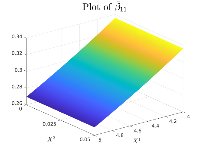
4.0.1 Plots of Drift and Diffusion Surfaces

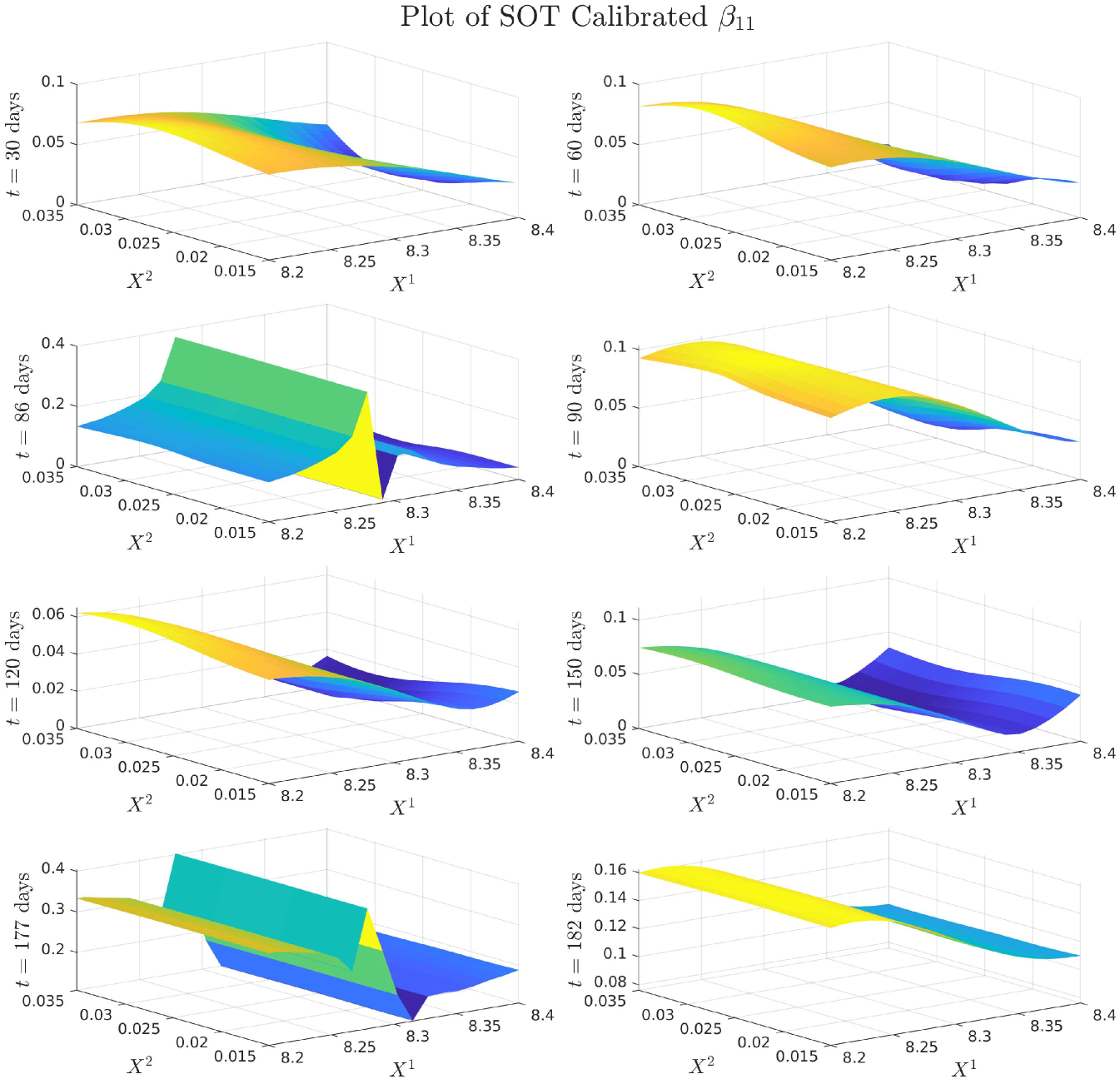
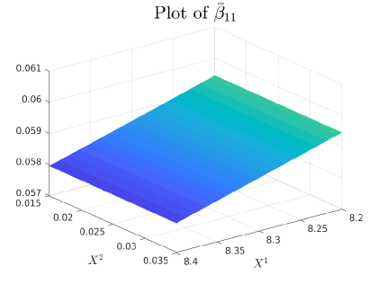
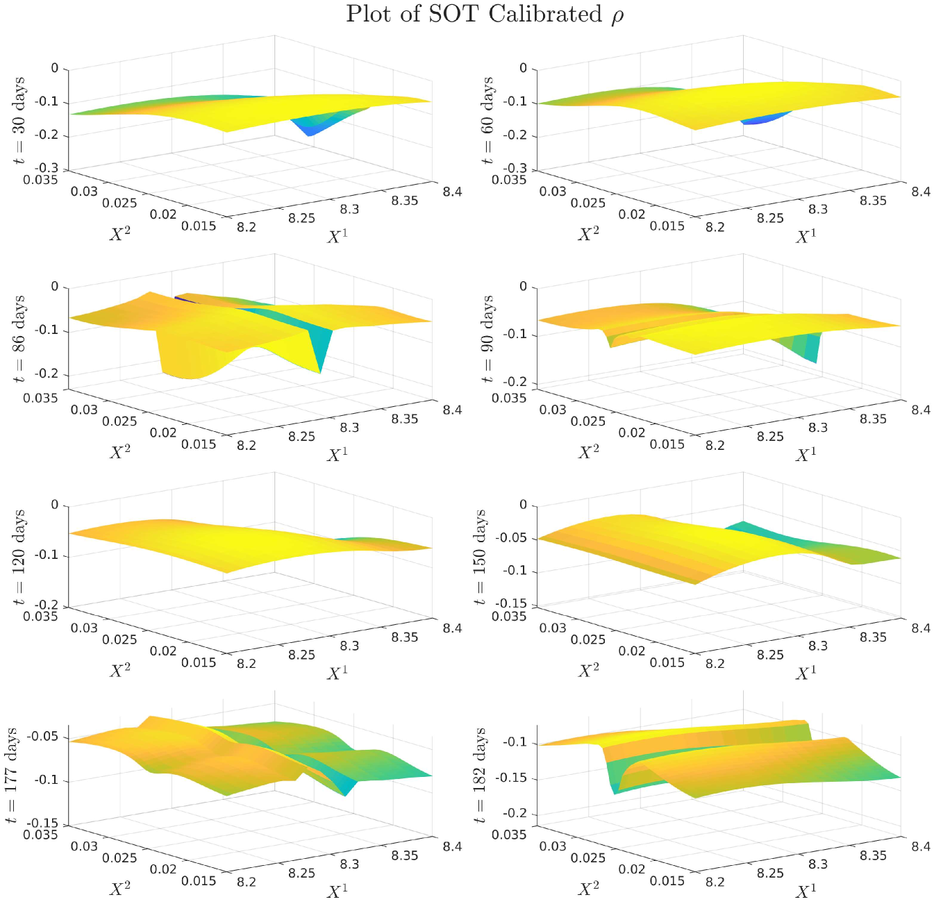
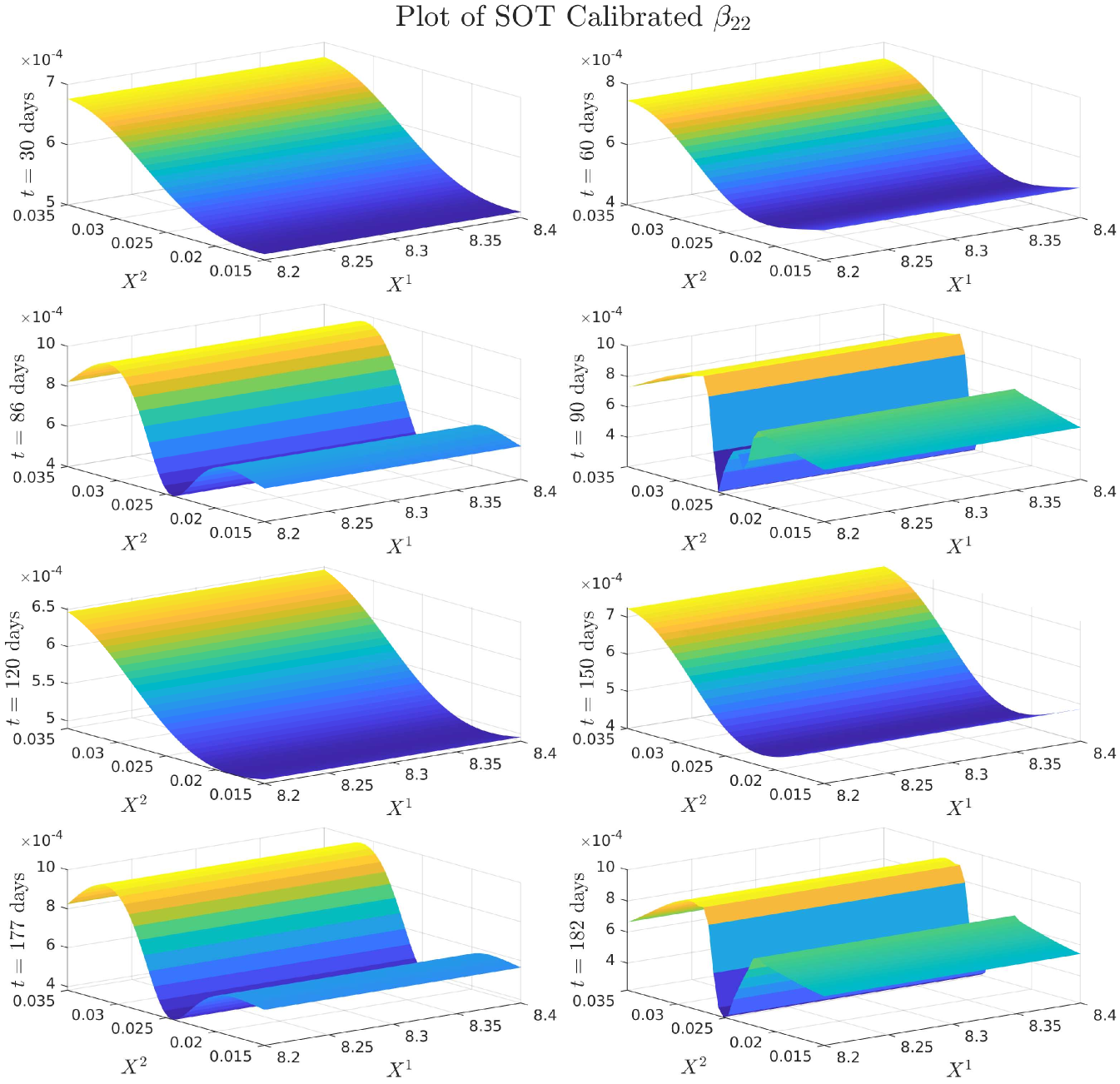
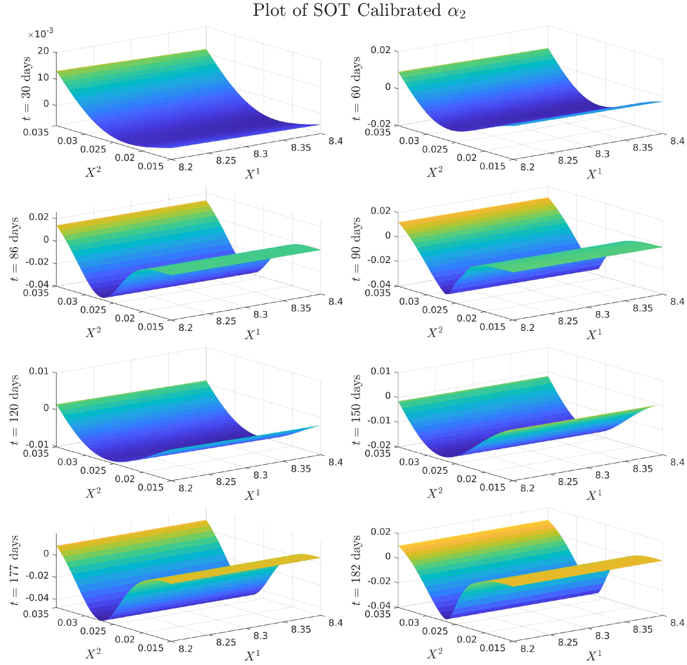
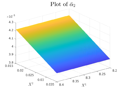
5 Numerical results: a comparison of three SOT Calibration approaches

Above we develop a joint calibration method for European options on a stock and on interest rates. In [18] a sequential approach was proposed in which the interest rates model was calibrated first and frozen for the subsequent calibration of a local volatility model for the stock prices. This was done under rigid restrictions on the structure of the correlation – it was conjectured this would speed up the numerics. We want to now compare the two approaches numerically, as well as introduce and compare a third approach which also proceeds sequentially but relaxes the assumptions on the correlation.

We test the methods on simulated data. We use the generating model as the reference model for the short rate. In the two cases where the interest rate is frozen, the surface plots of $\alpha_{2}$ and $\beta_{22}$ will remain the same as the reference model, however $\alpha_{2}$ and $\beta_{22}$ may be perturbed in the joint calibration case so we show all surface plots. Specifically, we take a Hull-White model for the interest rate, see [15, 16], and local volatility dynamics for the log-price:

$\displaystyle\mathop{}\!\mathrm{d}Z_{t}$	$\displaystyle=r_{t}-\frac{1}{2}\sigma^{2}(t,Z_{t},r_{t})+\sigma(t,Z_{t},r_{t})\mathop{}\!\mathrm{d}W^{1}_{t}$
$\displaystyle\mathop{}\!\mathrm{d}r_{t}$	$\displaystyle=(b(t)-ar_{t})\mathop{}\!\mathrm{d}t+\sigma_{r}\mathop{}\!\mathrm{d}W^{2}_{t}$	(20)
$\displaystyle\mathop{}\!\mathrm{d}\langle W^{1},W^{2}\rangle_{t}$	$\displaystyle=\rho(t,Z_{t},r_{t})\mathop{}\!\mathrm{d}t$

Where $a,\sigma_{r}(t)>0$ are constants and $b(\cdot)$ is a function of time, calibrated so that the dynamics of $(r_{t})_{0\leqslant t\leqslant T}$ match the market data (e.g., suitable interest rates caps and floors). Both $a$ and $\sigma_{r}$ being positive constants is not a particularly restrictive constraint as remarked in [3, 17]. Note that $b(t)$ will therefore need to be calibrated to fit the term structure of interest rates seen in the market. Our reference model for the local volatility of the log-stock will be a CEV model, as above.

The difference in the calibration approach for all three methods is what process(es) are being calibrated, or equivalently the cost function employed, which then also leads to different formulae for the optimal coefficients. We review briefly the sequential method used in [18] and define its extension, the “full sequential” method. We then provide numerical results comparing the three approaches.

5.1 Sequential Calibration

We fix a reference function $\rho_{\mathrm{ref}}(t,Z_{t},r_{t})\in\mathbb{R}^{2}$ and restrict correlation to the following representation:

\rho(t,Z_{t},r_{t})=\frac{\sigma_{r}(t)}{\sigma(t,Z_{t},r_{t})}\rho_{\mathrm{ref}}(t,Z_{t},r_{t}),\quad\text{for}\>t\in[0,T].

(21)

We then set:

\Gamma_{\mathrm{seq}}(t,r)=\left\{(\alpha,\beta)\in\mathbb{R}^{2}\times\mathbb{S}^{2}_{+}\>:\>\alpha_{1}=r-\frac{1}{2}\beta_{11},\>\alpha_{2}=(b(t)-ar),\>\beta_{12}=\beta_{21}=\rho_{\mathrm{ref}}\sigma_{r}^{2},\>\beta_{22}=\sigma_{r}^{2}\right\},

(22)

We also require the inequality $\rho_{\mathrm{ref}}(t,Z_{t},r_{t})^{2}\sigma_{r}(t)^{2}\leqslant\sigma^{2}(t,Z_{t},r_{t})$ to keep $\rho(t,Z_{t},r_{t})\in[-1,1]$ as a correlation also. Since $r_{t}$ is on a much lower scale to $Z_{t}$ , we have that $\sigma_{r}^{2}\ll\sigma^{2}$ , so this condition is not financially restrictive. To enforce this condition, we will define a convex function $H:\mathbb{R}\times\mathbb{R}^{+}\times\mathbb{R}\to\mathbb{R}\cup\{+\infty\}$ with a parameter $p>2$ :

H(x,\bar{x},s)\coloneqq\begin{cases}(p-1)\left(\frac{x-s}{\bar{x}-s}\right)^{1+p}+(p+1)\left(\frac{x-s}{\bar{x}-s}\right)^{1-p}-2p,&\text{if}\>x,\bar{x}>s,\\ +\infty,&\text{otherwise}.\end{cases}

The coefficients of each term ensure that $H(x,\bar{x},s)$ is minimised over $x$ at $x=\bar{x}$ with $\min_{x}H(x,\bar{x},s)=0$ . We fix a reference local volatility function $\bar{\sigma}^{2}=\bar{\sigma}^{2}(t,Z_{t},r_{t})$ that represents the desired model. Since we wish to penalise deviations away from our reference volatility $\overline{\sigma}^{2}$ , we define our cost function $F$ as follows:

F_{\mathrm{seq}}(t,r,\alpha,\beta)=\begin{cases}H(\beta_{11},\bar{\sigma}^{2},\rho_{\mathrm{ref}}^{2}\sigma_{r}^{2}),&\text{if}\>(\alpha,\beta)\in\Gamma_{\mathrm{seq}}(t,r),\\ +\infty,&\text{otherwise}.\end{cases}

(23)

With this cost function and the reference model fixed by $\Gamma_{\mathrm{seq}}$ in (22), our dual formulation becomes

Problem 5.1 (Sequential Dual Formulation).

V=\sup_{\lambda}\lambda\cdot u-\varphi^{\lambda}(0,Z_{0},r_{0}).

Where $\varphi^{\lambda}=\varphi(t,z,r)$ solves the HJB equation:

	$\displaystyle\sum_{i=1}^{n}\lambda_{i}G_{i}(x)\delta_{\tau_{i}}+\partial_{t}\varphi+$	$\displaystyle\sup_{\beta_{11}}\biggl{(}\left(r-\frac{1}{2}\beta_{11}\right)\partial_{z}\varphi+(b(t)-ar)\partial_{r}\varphi+\frac{1}{2}\beta_{11}\partial^{2}_{zz}\varphi+\rho_{\mathrm{ref}}\sigma_{r}^{2}\partial^{2}_{zr}\varphi+\frac{1}{2}\sigma^{2}_{r}\partial^{2}_{rr}\varphi-r\varphi$
		$\displaystyle\qquad\qquad-H(\beta_{11},\bar{\sigma}^{2},\rho_{\mathrm{ref}}^{2}\sigma_{r}^{2})\biggr{)}=0,\quad(t,z,r)\in[0,T]\times\mathbb{R}^{2}.$		(24)

Lemma 5.2 (Analytic Formula for the Optimal Characteristic in Sequential Calibration).

The optimal characteristic in the HJB equation (24), $\beta_{11}^{*}$ is given by

\beta_{11}^{*}(t,z,r)=\rho_{\mathrm{ref}}^{2}\sigma_{r}^{2}+\left(\frac{(\bar{\sigma}^{2}-\rho_{\mathrm{ref}}^{2}\sigma_{r}^{2})^{p}(\varphi_{zz}-\varphi_{z})}{4(p^{2}-1)}+\frac{1}{2}\sqrt{\left(\frac{(\bar{\sigma}^{2}-\rho_{\mathrm{ref}}^{2}\sigma_{r}^{2})^{p}(\varphi_{zz}-\varphi_{z})}{2(p^{2}-1)}\right)^{2}+4(\bar{\sigma}^{2}-\rho_{\mathrm{ref}}^{2}\sigma_{r}^{2})^{2p}}\right)^{\frac{1}{p}}.

(25)

We use $p=4$ in our numerical experiments, see Table 3.

5.2 “Full Sequential” Calibration

We introduce the notion of “full sequential” calibration, in which the correlation is treated as a free parameter rather than prescribed via (21). Our set $\Gamma$ now becomes:

\Gamma_{\text{full seq}}(t,r)=\left\{(\alpha,\beta)\in\mathbb{R}^{2}\times\mathbb{S}^{2}_{+}\>:\>\alpha_{1}=r-\frac{1}{2}\beta_{11},\>\alpha_{2}=(b(t)-ar),\>\beta_{22}=\sigma_{r}^{2}\right\}.

(26)

We use the same cost function as in joint calibration, however since we have from the definition of $\Gamma_{\text{full seq}}$ that $\alpha_{2}=\overline{\alpha}_{2}$ and $\beta_{22}=\overline{\beta}_{22}$ , and moreover that $\alpha_{1}-\overline{\alpha}_{1}=\frac{1}{2}(\overline{\beta}_{11}-\beta_{11})$ , our cost function will simplify to:

F_{\text{full seq}}(t,r,\alpha,\beta)=\begin{cases}\frac{5}{4}(\beta_{11}-\overline{\beta}_{11})^{2}+2(\beta_{12}-\overline{\beta}_{12})^{2},&\text{if }(\alpha,\beta)\in\Gamma_{\text{full seq}}(t,r),\\ +\infty,&\text{otherwise.}\end{cases}

(27)

Problem 5.3 (Full Sequential Dual Formulation).

V=\sup_{\lambda}\lambda\cdot u-\varphi^{\lambda}(0,Z_{0},r_{0}).

Where $\varphi^{\lambda}=\varphi(t,z,r)$ solves the HJB equation:

	$\displaystyle\sum_{i=1}^{n}\lambda_{i}G_{i}(x)\delta_{\tau_{i}}+\partial_{t}\varphi+$	$\displaystyle\sup_{\begin{subarray}{c}\beta_{11},\beta_{12},\\ \beta\in\mathbb{S}^{2}_{+}\end{subarray}}\biggl{(}\left(r-\frac{1}{2}\beta_{11}\right)\partial_{z}\varphi+(b(t)-ar)\partial_{r}\varphi+\frac{1}{2}\beta_{11}\partial^{2}_{zz}\varphi+\beta_{12}\partial^{2}_{zr}\varphi+\frac{1}{2}\sigma^{2}_{r}\partial^{2}_{rr}\varphi-r\varphi$
		$\displaystyle\qquad\qquad-F_{\text{full seq}}(t,r,\alpha,\beta)\biggr{)}=0,\quad(t,z,r)\in[0,T]\times\mathbb{R}^{2}.$		(28)

In a similar way to Lemma 3.2, we obtain an approximation of the optimal $\beta_{11}$ and $\beta_{12}$ by first optimising over $\beta_{11}$ , and then over $\beta_{12}$ applying the positive semidefinite constraint in this variable given $\beta_{11}^{*}$ .

Lemma 5.4.

Let $\beta_{22}^{*}=\sigma_{r}^{2}$ and define $\beta_{11}^{*}$ and $\beta_{12}^{*}=\beta_{21}^{*}$ by:

	$\displaystyle\beta_{11}^{*}(t,z,r)$	$\displaystyle=\begin{cases}\overline{\beta}_{11}(t,z,r)+\frac{1}{5}(\partial^{2}_{zz}\varphi(t,z,r)-\partial_{z}\varphi(t,z,r)),&\text{ when }\overline{\beta}_{11}+\frac{1}{5}(\partial^{2}_{zz}\varphi-\partial_{z}\varphi)\in[\delta_{11}^{l},\delta_{11}^{u}]\\ \delta_{11}^{l},&\text{ when }\overline{\beta}_{11}+\frac{1}{5}(\partial^{2}_{zz}\varphi-\partial_{z}\varphi)<\delta_{11}^{l},\\ \delta_{11}^{u},&\text{ when }\overline{\beta}_{11}+\frac{1}{5}(\partial^{2}_{zz}\varphi-\partial_{z}\varphi)>\delta_{11}^{u},\end{cases}$
	$\displaystyle\beta_{12}^{*}(t,z,r)$	$\displaystyle=\begin{cases}\overline{\beta}_{12}(t,z,r)+\frac{1}{4}\partial^{2}_{zr}\varphi(t,z,r),&\text{ when }\overline{\beta}_{12}+\frac{1}{4}\partial^{2}_{zr}\varphi\in\left[-\sigma_{r}\sqrt{\beta^{}_{11}},\sigma_{r}\sqrt{\beta^{}_{11}}\right],\\ -\sigma_{r}\sqrt{\beta^{}_{11}},&\text{ when }\overline{\beta}_{12}+\frac{1}{4}\partial^{2}_{zr}\varphi<-\sigma_{r}\sqrt{\beta^{}_{11}},\\ \sigma_{r}\sqrt{\beta^{}_{11}},&\text{ when }\overline{\beta}_{12}+\frac{1}{4}\partial^{2}_{zr}\varphi>\sigma_{r}\sqrt{\beta^{}_{11}}.\end{cases}$

Then $\beta^{*}$ is a positive semi-definite matrix and whenever

-\sigma_{r}\sqrt{\beta^{*}_{11}}<\beta^{*}_{12}<\sigma_{r}\sqrt{\beta^{*}_{11}}

then $\beta^{*}$ is the optimizer in (28).

5.3 Numerical Results

We solve Problem 5.1 and Problem 5.3 using the same methods as in Section 3.1. We provide a table of parameters used in the generating and reference models for our problem.

Hull-White CEV Model
Parameter	Value	Interpretation
$X^{1}_{0}$	$\log(92)$	Initial log-stock price
$X^{2}_{0}$	$0.025\times 100$	Initial short rate scaled by $R=100$
$\varepsilon_{1}$	$1\times 10^{-4}$	Tolerance for the difference in scaled model and market implied volatility
$\varepsilon_{2}$	$1\times 10^{-12}$	Tolerance for the policy iteration approximation of the optimal characteristics
$\delta_{11}^{l}$	0.05	Lower bound of $\beta_{11}$ in full sequential and joint calibration
$\delta_{11}^{u}$	1	Upper bound of $\beta_{11}$ in full sequential and joint calibration
$p$	4	Exponent in sequential calibration cost function
$\sigma$	0.60	Volatility scaling of generating CEV model
$\gamma$	0.95	Power law in generating CEV model
$b(t)$	$aX^{2}_{0}+\frac{\sigma_{r}^{2}}{2a}(1-e^{-2at})$	Initial term structure of Hull-White generating model
$a$	0.05	Speed of mean reversion of Hull-White generating model
$\sigma_{r}$	0.04	Volatility of Hull-White generating model
$\rho$	$-0.40$	Instantaneous correlation between short rate and log-stock in generating model
$\overline{\sigma}$	0.90	Volatility scaling of reference CEV model
$\overline{\gamma}$	0.89	Power law in reference CEV model
$\overline{b}(t)$	$\overline{a}X^{2}_{0}+\frac{\overline{\sigma}_{r}^{2}}{2\overline{a}}(1-e^{-2\overline{a}t})$	Initial term structure of Hull-White reference model
$\overline{a}$	0.05	Speed of mean reversion of Hull-White reference model
$\overline{\sigma}_{r}$	0.04	Volatility of Hull-White reference model
$\overline{\rho}$	$-0.20$	Instantaneous correlation between short rate and log-stock in reference model

Table 3: Parameter values of generating and reference models used in all three methods.

		Generating Model		Calibrated Model:		Calibrated Model:		Calibrated Model:
				Sequential		Full Sequential		Joint
Option Type	Strike	Price	IV	Price	IV	Price	IV	Price	IV
SPX Call options $t=60$ days	85	11.2142	0.4825	11.2139	0.4825	11.2139	0.4825	11.2152	0.4826
	92	7.3755	0.4811	7.3757	0.4811	7.3749	0.4811	7.3750	0.4811
	99	4.6051	0.4803	4.6045	0.4803	4.6038	0.4802	4.6056	0.4804
	106	2.7426	0.4799	2.7420	0.4798	2.7419	0.4798	2.7426	0.4799
	113	1.5667	0.4797	1.5665	0.4797	1.5667	0.4797	1.5673	0.4797
	120	0.8624	0.4795	0.8623	0.4795	0.8629	0.4796	0.8626	0.4796
SPX Call options $t=120$ days	85	14.0842	0.4821	14.0839	0.4821	14.0838	0.4821	14.0857	0.4822
	92	10.502	0.4809	10.5021	0.4809	10.5007	0.4808	10.5027	0.4809
	99	7.6696	0.4797	7.6712	0.4798	7.6699	0.4798	7.6691	0.4797
	106	5.4943	0.4785	5.4952	0.4785	5.4936	0.4784	5.4952	0.4785
	113	3.8607	0.4767	3.8609	0.4768	3.8597	0.4767	3.8594	0.4767
	120	2.6499	0.4738	2.6498	0.4738	2.6495	0.4738	2.6499	0.4738

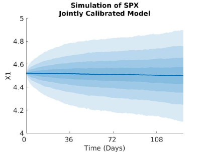
Table 4: Table of the generating and calibrated model prices and implied volatilities.

5.3.1 Implied Volatility and Monte Carlo Plots

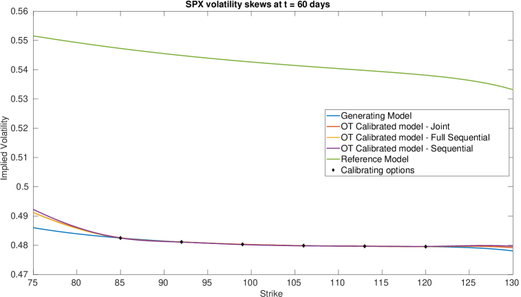
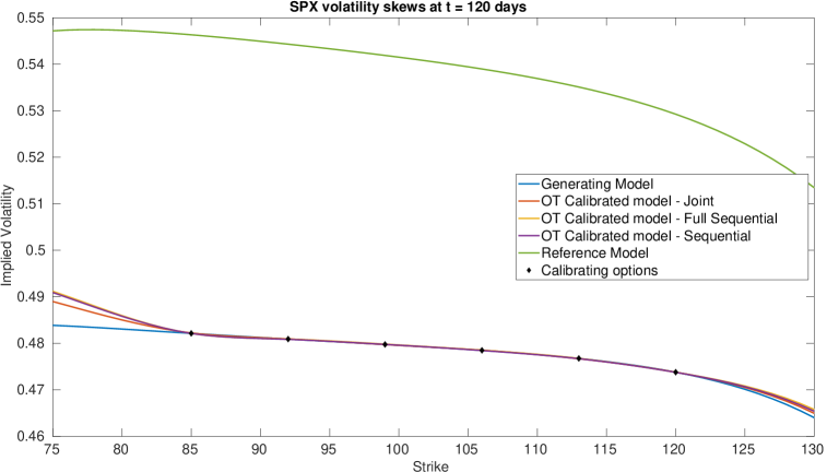
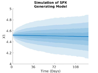
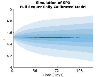
5.3.2 Plots of the Volatility and Correlation surfaces

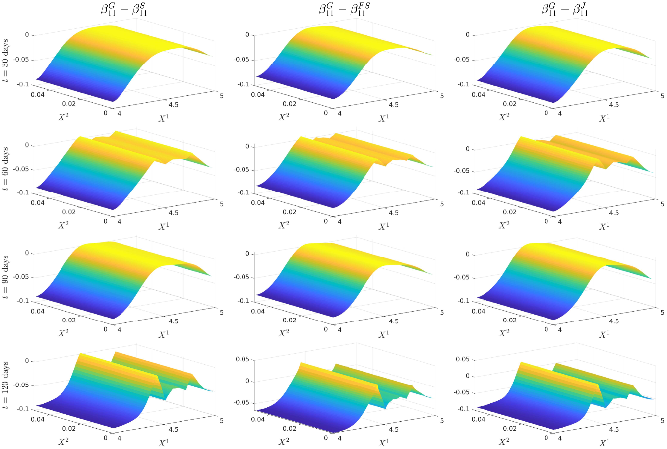
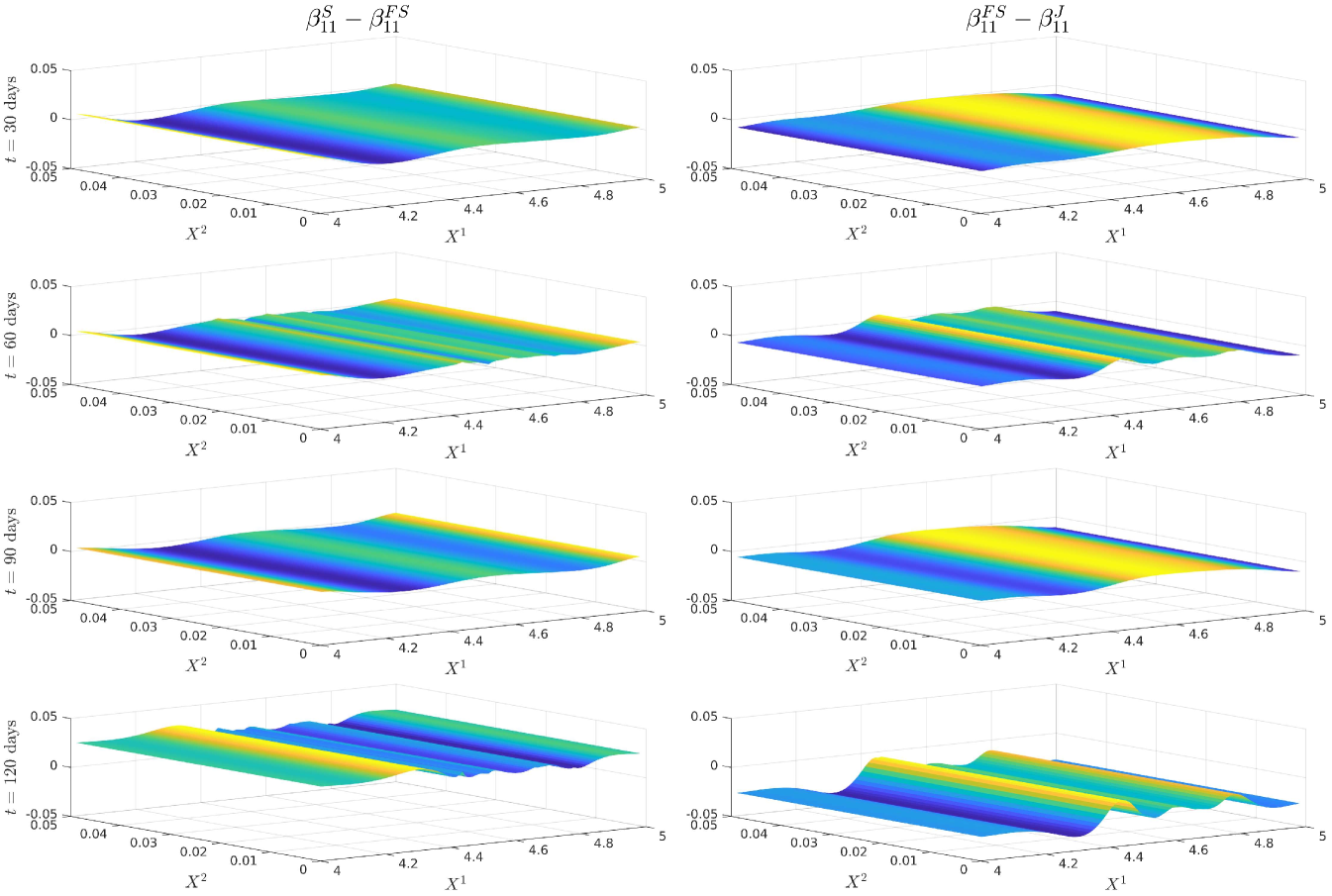
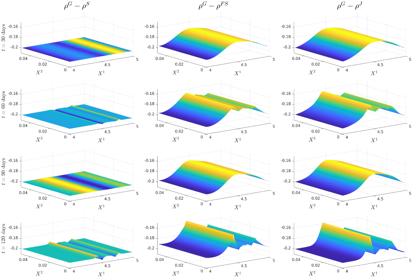
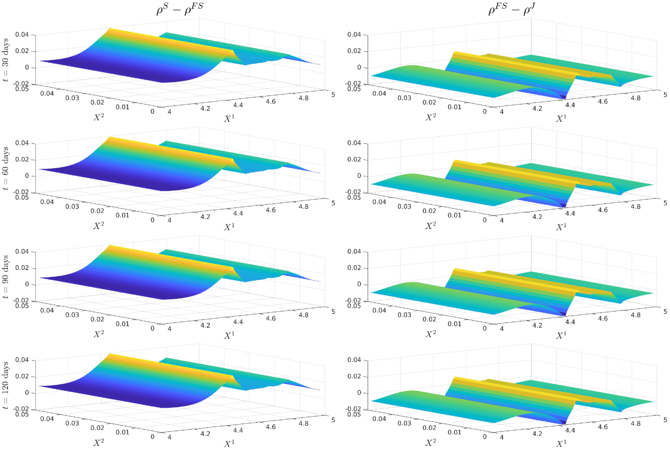
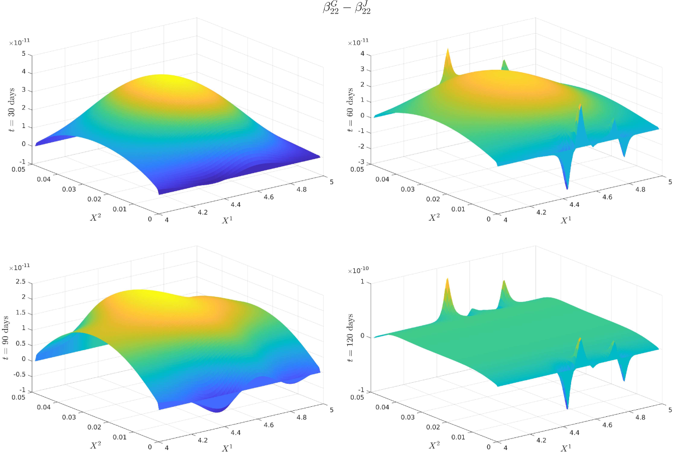
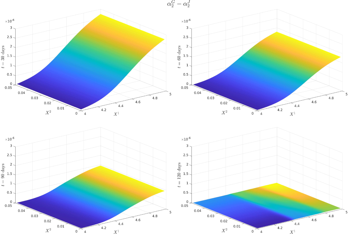
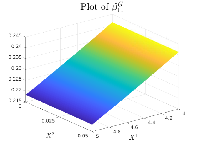
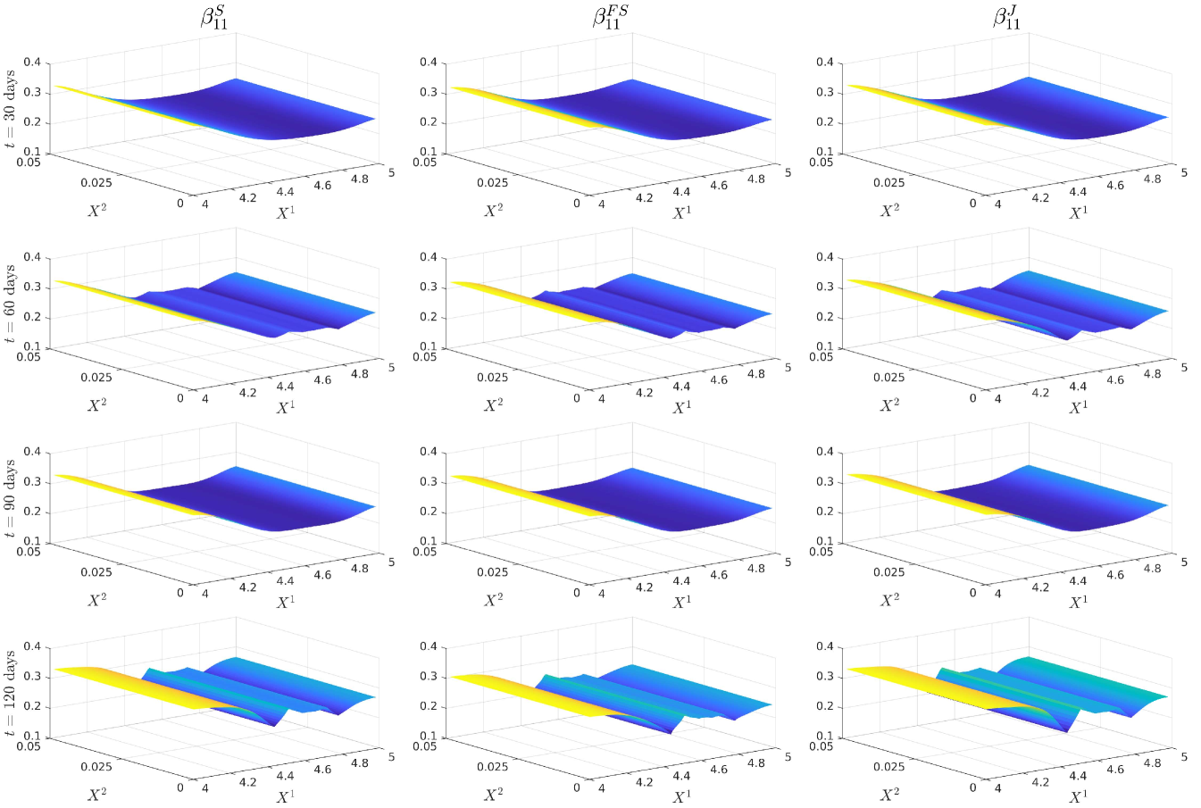
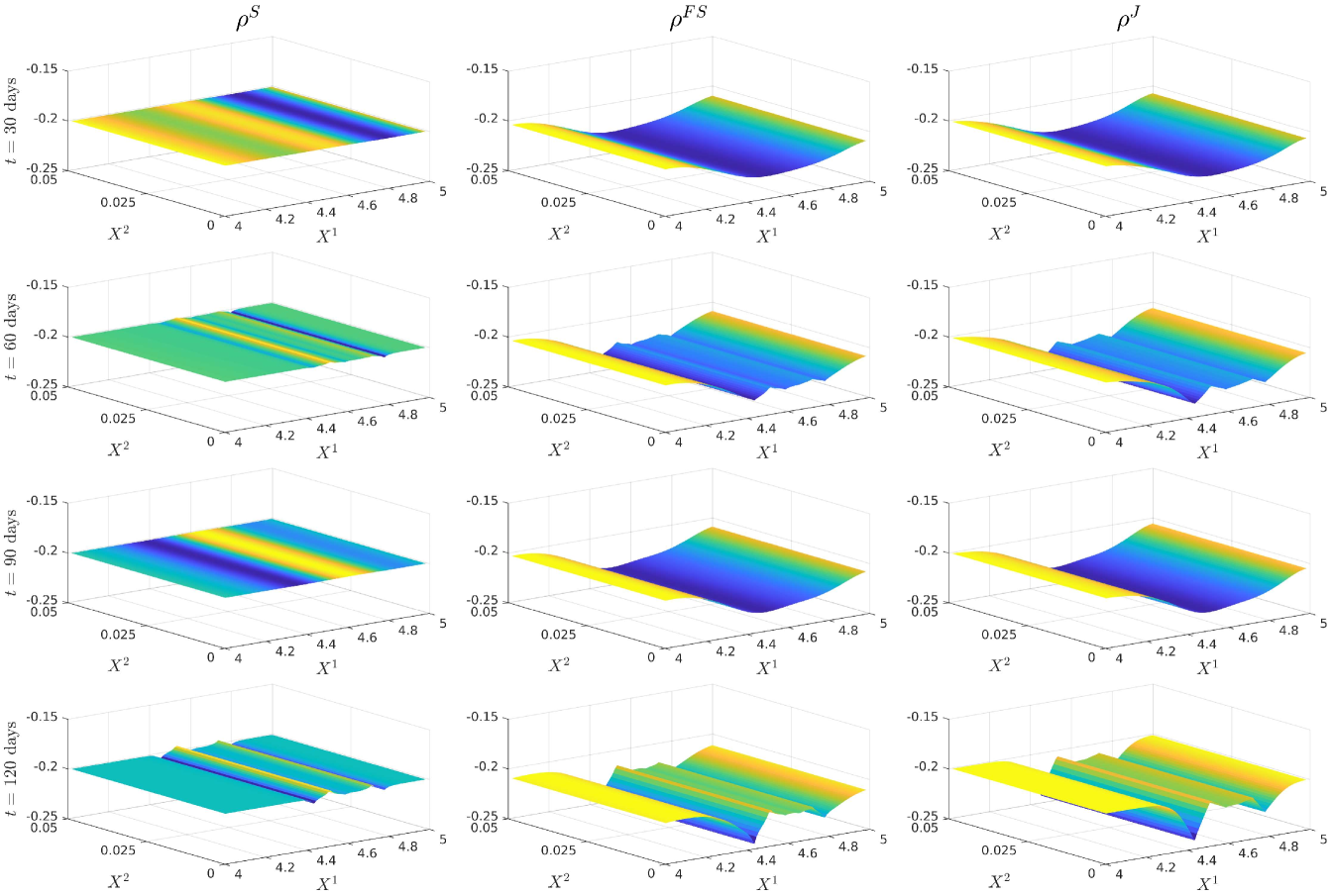
For notational ease in the comparison, denote via a superscript $S,FS,J,G$ the characteristic under the SOT sequential calibrated model, SOT full sequential calibrated model, SOT jointly calibrated model and generating model respectively. In order to provide a meaningful comparison of the three methods, we show plots of the difference in the surfaces for all five characteristics, and how all of them differ from the generating model. Plots of the actual surfaces are left in the appendix. We omit all plots for $\alpha_{1}$ since in all three cases it is entirely specified by $\beta_{11}$ . We remark that the formulae for $\beta_{11}^{FS}$ and $\beta_{11}^{J}$ given in Lemma 3.2 and Lemma 5.4 are upon a first glance the same, and both differ from the formula for $\beta_{11}^{S}$ given in (25). However, owing to the different cost functions and the fact that the joint problem allows for perturbations in the interest rate, whereas the full sequential problem does not, there is no expectation of the optimisers $\varphi^{*}_{FS}$ and $\varphi^{*}_{J}$ being the same since the global optimisers of both problems may differ. We expect the correlation coefficient $\rho^{S}$ to be almost constant and close to the reference model, owing to the assumption on the correlation in (21), whereas we expect some deviation away from the reference model for $\rho^{FS}$ and $\rho^{J}$ since we relax the assumptions on the correlation. The short rate volatility $\beta_{22}$ and short rate drift $\alpha_{2}$ are assumed to be a priori correct due to the matching generating and reference models. Note that the coefficients $\alpha_{2}^{S},\alpha_{2}^{FS},\beta_{22}^{S},\beta_{22}^{FS}$ are all fixed, and equal to these in the generating model, which we recall is also the reference model, i.e., we have²²2We confirmed this numerically in our results. $\alpha_{2}^{S}=\alpha_{2}^{FS}=\alpha_{2}^{G}$ and $\beta_{22}^{S}=\beta_{22}^{FS}=\beta_{22}^{G}$ . However, in the joint calibration case we do not fix $\alpha_{2}^{J}$ and $\beta_{22}^{J}$ and our optimisers given in Lemma 3.2 do not guarantee replication of the generating model. Nonetheless, since the cost function penalises deviations from the reference model, we expect that $\alpha_{2}^{J}$ and $\beta_{22}^{J}$ will be close to the generating model with some small perturbations away fro $\alpha_{2}^{G}$ and $\beta_{22}^{G}$ .

5.4 Discussion of the results

Figure 12 (a) demonstrates that $\beta_{11}^{S},\beta_{11}^{FS},\beta_{11}^{J}$ all are near the generating model within the region of our strikes and then deviate in the same manner towards the reference model outside the region of calibrating call option strikes. This is expected behaviour since in all three cases, the cost functions penalise deviations away from a reference model volatility while enforcing that the observed call option prices are replicated. A remarkable result is that Figure 12 (b) shows that $\beta_{11}^{S},\beta_{11}^{FS},\beta_{11}^{J}$ are all close at $t=30,60,90$ days despite being defined differently. We do however see some expected perturbations on those dates and a larger perturbation at $t=120$ days which is also observed in the larger fluctuations seen in Figure 12 (a). Figure 13 (a) demonstrates strong dependence on the reference model: $\rho^{S},\rho^{FS},\rho^{J}$ all differ from $\rho^{G}$ by approximately $-0.2$ , however $\rho^{FS}$ and $\rho^{J}$ do perturb slightly towards to generating model in the region of strikes. Since our calibrating option has a payoff function only explicitly depending on the log-stock, this was expected behaviour since $\rho^{FS}$ and $\rho^{J}$ are defined via $\partial^{2}_{zr}\varphi$ . As remarked in [18], the extremely strong dependence on the reference model for $\rho^{S}$ arises mainly from the assumption on the form of the correlation given in (21). The differences observed in Figure 13 (b) arise from a fundamentally different handling of $\rho^{S}$ and that the volatility of the short rate is fixed so that $\rho^{FS}$ will be different to $\rho^{J}$ . Nonetheless, since all three depend strongly on the reference model, these fluctuations are small.

All three methods converged to a good accuracy with a maximum error in implied volatility of $10^{-4}$ , as shown in Table 4 and Figure 10, where in all three cases, we applied Algorithm 1 with the smoothed reference model iteration. A minimum of 10 smoothing iterations were applied in all three cases to generate smoother surfaces. Since each smoothing iteration terminates either when calibration error is achieved or when a threshold of function evaluations were attained, in practice around 20 were required for the sequential calibration case to converge, as opposed to full sequential and joint calibration which both converged on the $10^{\mathrm{th}}$ smoothing iteration. The fastest in terms of computational time was the full sequential approach, taking just over an hour and the slowest was the joint calibration approach taking around three hours. Each epoch of a smoothed reference iteration was the fastest in sequential calibration. Joint calibration being the slowest was to be expected since it still computes the optimisers $\alpha^{*}_{2}$ and $\beta^{*}_{22}$ at each point, which is more expensive that simply fixing them as in the other two methods.

Appendix A Plots of Calibrated Characteristics from the Comparison

We only show the plots of $\beta_{11}$ and $\rho$ since $\alpha_{1}$ is entirely determined by $\beta_{11}$ and Figure 12 and Figure 15 demonstrate that all three cases are extremely close or exactly equal to the generating model for $\beta_{22}$ and $\alpha_{2}$ .

Appendix B Proof of Lemma 3.2

Since $\Gamma$ defined in (7) enforces that $\alpha^{*}_{1}=r-\frac{1}{2}\beta^{*}_{11}$ , we immediately have the first equality given an optimiser $\beta^{*}_{11}$ . We remark that any reference model $(\overline{\alpha},\overline{\beta})$ will also follow the same constraint. Additionally, $\beta\in\mathbb{S}^{2}_{+}$ is enforced by the set $\Gamma$ . Therefore, since our cost function is given by (8), its Legendre-Fenchel transform $F^{*}:\mathbb{R}^{2}\times\mathbb{S}^{2}\to\mathbb{R}$ is given by:

	$\displaystyle F^{*}(a,b)$	$\displaystyle=\sup_{\begin{subarray}{c}\alpha_{2}\in\mathbb{R},\\ \beta\in\mathbb{S}^{2}_{+},\\ \beta_{11}\in[\delta_{11}^{l},\delta_{11}^{u}],\\ \beta_{22}\in[\delta_{22}^{l},\delta_{22}^{u}]\end{subarray}}\biggl{\{}a_{1}\left(r-\frac{1}{2}\beta_{11}\right)+a_{2}\alpha_{2}+b_{11}\beta_{11}+2b_{12}\beta_{12}+b_{22}\beta_{22}-\frac{1}{4}(\beta_{11}-\overline{\beta}_{11})^{2}-(\alpha_{2}-\overline{\alpha}_{2})^{2}$
		$\displaystyle\qquad\qquad\qquad\qquad-(\beta_{11}-\overline{\beta}_{11})^{2}-2(\beta_{12}-\overline{\beta}_{12})^{2}-(\beta_{22}-\overline{\beta}_{22})^{2}\biggr{\}}$		(29)

The gradient $\nabla F^{*}(a,b)$ is given by the maximisers of (29), and by rearranging the $\alpha_{2}$ term, we obtain the second equality:

\alpha_{2}^{*}=\operatorname*{arg\,max}_{\alpha_{2}\in\mathbb{R}}\left\{a_{2}\alpha_{2}-\alpha_{2}^{2}+2\alpha_{2}\overline{\alpha}_{2}-\overline{\alpha}^{2}_{2}\right\}=\operatorname*{arg\,min}_{\alpha_{2}\in\mathbb{R}}\left\{\left(\alpha_{2}-\left(\overline{\alpha}_{2}+\frac{1}{2}a_{2}\right)\right)^{2}\right\}=\overline{\alpha}_{2}+\frac{1}{2}a_{2}.

Now, similarly rearranging (29)

	$\displaystyle[\beta_{12}^{},\beta_{11}^{},\beta_{22}^{*}]$	$\displaystyle=\operatorname{arg\,min}_{\begin{subarray}{c}\beta_{12}\\ \beta\in\mathbb{S}^{2}_{+}\end{subarray}}\Biggl{\{}\Biggl{[}\left(\beta_{12}-\left(\overline{\beta}_{12}+\frac{1}{2}b_{12}\right)\right)^{2},\operatorname{arg\,min}_{\begin{subarray}{c}\beta_{11}\\ \beta_{11}\in[\delta_{11}^{l},\delta_{11}^{u}]\end{subarray}}\left\{\left(\beta_{11}-\left(\overline{\beta}_{11}+\frac{1}{5}\left(2b_{11}-a_{1}\right)\right)\right)^{2}\right\},$
		$\displaystyle\qquad\qquad\qquad\qquad\operatorname*{arg\,min}_{\begin{subarray}{c}\beta_{22}\\ \beta_{22}\in[\delta_{22}^{l},\delta_{22}^{u}]\end{subarray}}\left\{\left(\beta_{22}-\left(\overline{\beta}_{22}+\frac{1}{2}b_{22}\right)\right)^{2}\right\}\Biggr{]}\Biggr{\}}$

We solve the minimisations of $\beta_{11}$ and $\beta_{22}$ inside the $\beta_{12}$ minimisation problem by taking:

	$\displaystyle\beta^{*}_{11}$	$\displaystyle=\begin{cases}\overline{\beta}_{11}+\frac{1}{5}(2b_{11}-a_{1}),&\text{ if }\overline{\beta}_{11}+\frac{1}{5}(2b_{11}-a_{1})\in[\delta_{11}^{l},\delta_{11}^{u}]\\ \delta_{11}^{u},&\text{ if }\overline{\beta}_{11}+\frac{1}{5}(2b_{11}-a_{1})>\delta_{11}^{u}\\ \delta_{11}^{l},&\text{ if }\overline{\beta}_{11}+\frac{1}{5}(2b_{11}-a_{1})<\delta_{11}^{l}\end{cases}$
	$\displaystyle\beta^{*}_{22}$	$\displaystyle=\begin{cases}\overline{\beta}_{22}+\frac{1}{2}b_{22},&\text{ if }\overline{\beta}_{22}+\frac{1}{2}b_{22}\in[\delta_{22}^{l},\delta_{22}^{u}],\\ \delta_{22}^{u},&\text{ if }\overline{\beta}_{22}+\frac{1}{2}b_{22}>\delta_{22}^{u},\\ \delta_{22}^{l},&\text{ if }\overline{\beta}_{22}+\frac{1}{2}b_{22}<\delta_{22}^{l}.\end{cases}$

Given $\beta^{*}_{11}$ and $\beta^{*}_{22}$ as above, we now may rewrite the outside constraint as $\beta_{12}\in[-\sqrt{\beta^{*}_{11}\beta^{*}_{22}},\sqrt{\beta^{*}_{11},\beta^{*}_{22}}]$ and thus obtain:

\beta^{*}_{12}=\begin{cases}\overline{\beta}_{12}+\frac{1}{2}b_{12},&\text{ if }\overline{\beta}_{12}+\frac{1}{2}b_{12}\in[-\sqrt{\beta^{*}_{11}\beta^{*}_{22}},\sqrt{\beta^{*}_{11}\beta^{*}_{22}}],\\ \sqrt{\beta^{*}_{11}\beta^{*}_{22}},&\text{ if }\overline{\beta}_{12}+\frac{1}{2}b_{12}>\sqrt{\beta^{*}_{11}\beta^{*}_{22}},\\ -\sqrt{\beta^{*}_{11}\beta^{*}_{22}},&\text{ if }\overline{\beta}_{12}+\frac{1}{2}b_{12}<-\sqrt{\beta^{*}_{11}\beta^{*}_{22}}.\end{cases}

In particular, in the first case, the condition $\beta\in\mathbb{S}^{2}_{+}$ is automatically satisfied and the procedure returns the optimizer. By taking $a=\nabla_{x}\varphi$ and $b=\frac{1}{2}\nabla_{x}^{2}\varphi$ , we conclude the proof.

Appendix C Application of Full Sequential Calibration to Local-Stochastic Volatility Models

We observe there that the method of Section 5.2 can be applied to the local-stochatic volatility calibration setting of [12] to relax the constraint on the correlation imposed in that paper. In this setting, we assume our interest rate is zero and that our reference model is given by a Heston model, derived in [14]. The state variables are therefore our log-stock and a correlated stochastic term for the volatility, with dynamics given by:

	$\displaystyle\mathop{}\!\mathrm{d}Z_{t}$	$\displaystyle=-\frac{1}{2}V_{t}\mathop{}\!\mathrm{d}t+\sqrt{V_{t}}\mathop{}\!\mathrm{d}W_{t}^{1},$
	$\displaystyle\mathop{}\!\mathrm{d}V_{t}$	$\displaystyle=\kappa(\theta-V_{t})\mathop{}\!\mathrm{d}t+\xi\sqrt{V_{t}}\mathop{}\!\mathrm{d}W^{2}_{t},$
	$\displaystyle\mathop{}\!\mathrm{d}\langle W^{1},W^{2}\rangle_{t}$	$\displaystyle=\rho\mathop{}\!\mathrm{d}t,$

where $\kappa,\theta,\xi>0$ and $\rho\in[-1,1]$ . We assume that the state variable $V_{t}$ is known, so the model characteristics that we want to calibrate are the volatility of the log-stock and the correlation between the state variables. As before, the instruments that we calibrate this model to are European call options on the chosen stock. We now define our cost function in a similar manner to Section 5.2 by defining the convex set $\Gamma_{\mathrm{LSV}}$ :

\Gamma_{\text{LSV}}(v)=\left\{(\alpha,\beta)\in\mathbb{R}^{2}\times\mathbb{S}^{2}_{+}\>:\>\alpha_{1}=-\frac{1}{2}\beta_{11},\>\alpha_{2}=\kappa(\theta-v),\>\beta_{22}=\xi^{2}v,\>\delta_{11}^{l}\leqslant\beta_{11}\leqslant\delta_{11}^{u}\right\}.

(30)

F_{\text{LSV}}(v,\alpha,\beta)=\begin{cases}\frac{5}{4}(\beta_{11}-\overline{\beta}_{11})^{2}+2(\beta_{12}-\overline{\beta}_{12})^{2},&\text{if }(\alpha,\beta)\in\Gamma_{\text{LSV}}(v),\\ +\infty,&\text{otherwise.}\end{cases}

(31)

Since we have no stochastic discount factor, we no longer need the sub-probability measure approach of [18], and therefore can directly apply the duality result of [12, Proposition 3.7]. With our cost function defined in (31), we therefore obtain the following dual formulation:

Problem C.1 (Full Sequential Dual Formulation).

V=\sup_{\lambda}\lambda\cdot u-\varphi^{\lambda}(0,Z_{0},V_{0}).

Where $\varphi^{\lambda}=\varphi(t,z,v)$ solves the HJB equation:

	$\displaystyle\sum_{i=1}^{n}\lambda_{i}G_{i}(x)\delta_{\tau_{i}}+\partial_{t}\varphi+$	$\displaystyle\sup_{\begin{subarray}{c}\beta_{11},\beta_{12},\\ \beta\in\mathbb{S}^{2}_{+}\end{subarray}}\biggl{(}-\frac{1}{2}\beta_{11}\partial_{z}\varphi+\kappa(\theta-v)\partial_{v}\varphi+\frac{1}{2}\beta_{11}\partial^{2}_{zz}\varphi+\beta_{12}\partial^{2}_{zv}\varphi+\frac{1}{2}\xi^{2}v\partial^{2}_{vv}\varphi$
		$\displaystyle\qquad\qquad-F_{\mathrm{LSV}}(v,\alpha,\beta)\biggr{)}=0,\quad(t,z,v)\in[0,T]\times\mathbb{R}^{2}.$		(32)

Similar to Lemma 5.4, we obtain the following approximation for $\beta^{*}_{11}$ and $\beta^{*}_{12}$ :

Lemma C.2.

Let $\beta^{*}_{22}=\xi^{2}v$ and define $\beta_{11}^{*}$ and $\beta_{12}^{*}=\beta^{*}_{21}$ by

	$\displaystyle\beta_{11}^{*}(t,z,v)$	$\displaystyle=\begin{cases}\overline{\beta}_{11}(t,z,v)+\frac{1}{5}(\partial^{2}_{zz}\varphi(t,z,v)-\partial_{z}\varphi(t,z,v)),&\text{ when }\overline{\beta}_{11}+\frac{1}{5}(\partial^{2}_{zz}\varphi-\partial_{z}\varphi)\in[\delta_{11}^{l},\delta_{11}^{u}]\\ \delta_{11}^{l},&\text{ when }\overline{\beta}_{11}+\frac{1}{5}(\partial^{2}_{zz}\varphi-\partial_{z}\varphi)<\delta_{11}^{l},\\ \delta_{11}^{u},&\text{ when }\overline{\beta}_{11}+\frac{1}{5}(\partial^{2}_{zz}\varphi-\partial_{z}\varphi)>\delta_{11}^{u},\end{cases}$
	$\displaystyle\beta_{12}^{*}(t,z,v)$	$\displaystyle=\begin{cases}\overline{\beta}_{12}(t,z,v)+\frac{1}{4}\partial^{2}_{zv}\varphi(t,z,v),&\text{ when }\overline{\beta}_{12}+\frac{1}{4}\partial^{2}_{zv}\varphi\in\left[-\xi\sqrt{v\beta^{}_{11}},\xi\sqrt{v\beta^{}_{11}}\right],\\ -\xi\sqrt{v\beta^{}_{11}},&\text{ when }\overline{\beta}_{12}+\frac{1}{4}\partial^{2}_{zv}\varphi<-\xi\sqrt{v\beta^{}_{11}},\\ \xi\sqrt{v\beta^{}_{11}},&\text{ when }\overline{\beta}_{12}+\frac{1}{4}\partial^{2}_{zv}\varphi>\xi\sqrt{v\beta^{}_{11}}.\end{cases}$

Then $\beta^{*}$ is a positive semi-definite matrix and whenever

-\xi\sqrt{v\beta^{*}_{11}}<\beta^{*}_{12}<\xi\sqrt{v\beta^{*}_{11}}

then $\beta^{*}$ is the optimizer in (32).

We numerically solve this problem using the same methods as in Section 3.1, we show a table of parameters below. We simulate the call option prices from the generating model and test it against two reference models: a “good” reference model and a “bad” reference model. The parameters used in $\Gamma_{\mathrm{LSV}}$ are those of the reference model.

Heston Model
Parameter	Value	Interpretation
$X^{1}_{0}$	$\log(92)$	Initial log-stock price
$X^{2}_{0}$	$0.25$	Initial volatility
$\varepsilon_{1}$	$1\times 10^{-4}$	Tolerance for the difference in scaled model and market implied volatility
$\varepsilon_{2}$	$1\times 10^{-12}$	Tolerance for the policy iteration approximation of the optimal characteristics
$\kappa$	1	Speed of volatility mean reversion in the generating model
$\theta$	0.05	Long-term mean of the volatility in the generating model
$\xi$	0.2	Volatility scaling of the volatility in the generating model
$\rho$	-0.4	Instantaneous correlation between the log-stock and volatility in the generating model
$\overline{\kappa}_{\mathrm{good}}$	1.5	Speed of volatility mean reversion in the reference model
$\overline{\theta}_{\mathrm{good}}$	0.07	Long-term mean of the volatility in the reference model
$\overline{\xi}_{\mathrm{good}}$	0.15	Volatility scaling of the volatility in the reference model
$\overline{\rho}_{\mathrm{good}}$	-0.2	Instantaneous correlation between the log-stock and volatility in the reference model
$\overline{\kappa}_{\mathrm{bad}}$	2	Speed of volatility mean reversion in the reference model
$\overline{\theta}_{\mathrm{bad}}$	0.09	Long-term mean of the volatility in the reference model
$\overline{\xi}_{\mathrm{bad}}$	0.3	Volatility scaling of the volatility in the reference model
$\overline{\rho}_{\mathrm{bad}}$	0.2	Instantaneous correlation between the log-stock and volatility in the reference model

Table 5: Parameter values of generating and reference models used in the LSV calibration.

		Generating Model		Calibrated Model:		Calibrated Model:
				Good Reference		Bad Reference
Option Type	Strike	Price	IV	Price	IV	Price	IV
SPX Call options $t=60$ days	85	11.0144	0.4840	11.0143	0.4840	11.0148	0.4841
	92	7.1928	0.4808	7.1928	0.4808	7.1920	0.4808
	99	4.4416	0.4782	4.4419	0.4782	4.4414	0.4782
	106	2.6037	0.4761	2.6036	0.4761	2.6034	0.4760
	113	1.4564	0.4744	1.4562	0.4743	1.4562	0.4743
	120	0.7813	0.4729	0.7814	0.4730	0.7811	0.4729
SPX Call options $t=120$ days	85	13.4256	0.4686	13.4260	0.4687	13.4256	0.4686
	92	9.8367	0.4656	9.8372	0.4656	9.8370	0.4656
	99	7.0267	0.4628	7.0273	0.4628	7.0250	0.4627
	106	4.9025	0.4601	4.9043	0.4602	4.9034	0.4602
	113	3.3437	0.4574	3.3450	0.4575	3.3451	0.4575
	120	2.2243	0.4541	2.2249	0.4541	2.2252	0.4541

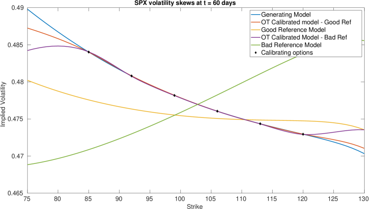
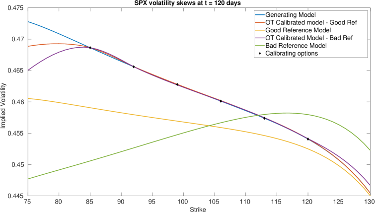
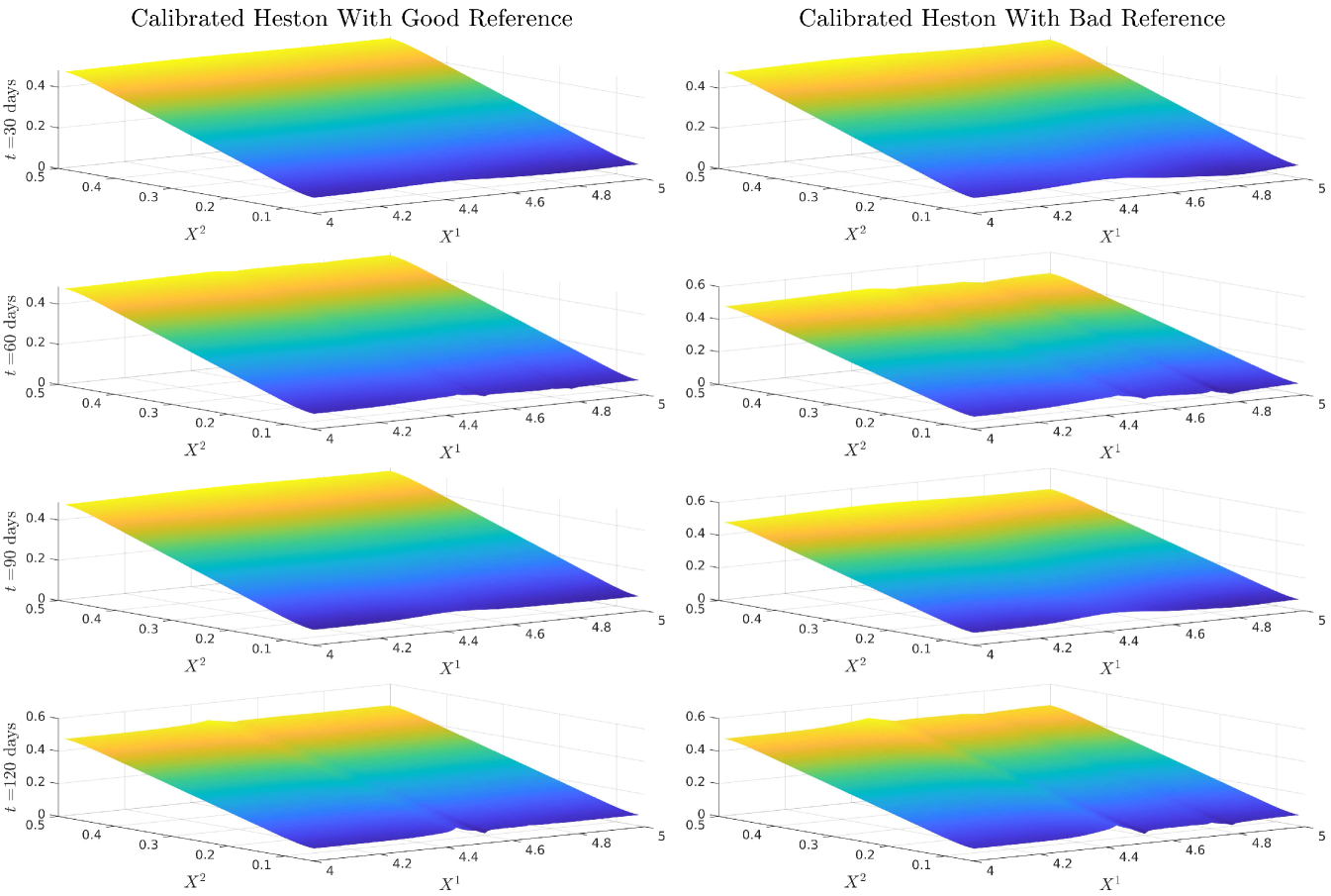
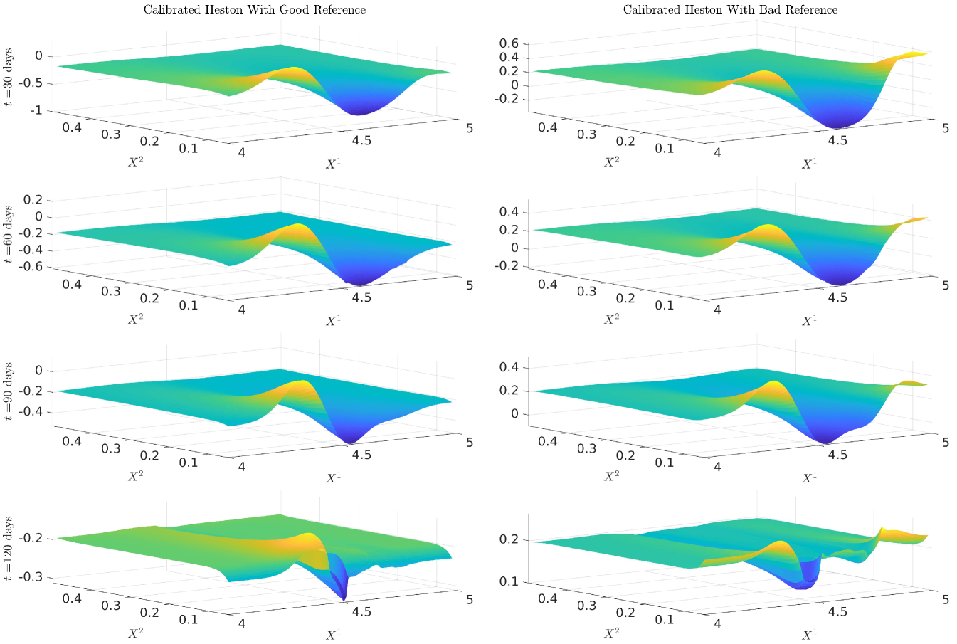
Table 6: Table of the generating and calibrated model prices and implied volatilities.

We remark that this approach can recover the implied volatility within the range of the strikes even when the reference model has completely the wrong shape of implied volatility. We now display the surfaces of SOT calibrated $\beta_{11}$ and $\rho$ . We notice that while the generating and reference models in $\beta_{11}$ are the same, our calibrated model is perturbed from the reference. We also notice that our calibrated correlation $\rho$ is close to the reference model correlation parameter in both cases, with deviations towards the generating model when we are in the range of our strikes and when $V_{t}$ is near zero. This strong dependence is also seen in our previous calibration approaches, and thus a good a priori estimate of $\rho$ would be needed in practice.

References

[1] Marco Avellaneda, Craig Friedman, Richard Holmes and Dominick Samperi “Calibrating volatility surfaces via relative-entropy minimization” In Applied Mathematical Finance 4.1 Taylor & Francis, 1997, pp. 37–64
[2] Jean-David Benamou and Yann Brenier “A computational fluid mechanics solution to the Monge-Kantorovich mass transfer problem” In Numerische Mathematik 84.3 Springer, 2000, pp. 375–393
[3] Damiano Brigo and Fabio Mercurio “Interest rate models-theory and practice: with smile, inflation and credit” Springer Science & Business Media, 2007
[4] Gerard Brunick and Steven Shreve “Mimicking an Itô process by a solution of a stochastic differential equation” In Annals of Applied Probability 23.4 Institute of Mathematical Statistics, 2013, pp. 1584–1628
[5] Lucilla Corrias “Fast Legendre–Fenchel transform and applications to Hamilton–Jacobi equations and conservation laws” In SIAM journal on numerical analysis 33.4 SIAM, 1996, pp. 1534–1558
[6] John Cox “Notes on option pricing I: Constant elasticity of variance diffusions” In Unpublished note, Stanford University, Graduate School of Business, 1975
[7] John Cox “The constant elasticity of variance option pricing model” In Journal of Portfolio Management Pageant Media, 1996, pp. 15–17
[8] Ivan Guo and Grégoire Loeper “Path dependent optimal transport and model calibration on exotic derivatives” In The Annals of Applied Probability 31.3 Institute of Mathematical Statistics, 2021, pp. 1232–1263
[9] Ivan Guo, Grégoire Loeper, Jan Obłój and Shiyi Wang “Joint Modeling and Calibration of SPX and VIX by Optimal Transport” In SIAM Journal on Financial Mathematics 13.1 SIAM, 2022, pp. 1–31
[10] Ivan Guo, Grégoire Loeper, Jan Obłój and Shiyi Wang “Optimal transport for model calibration” In Risk Magazine Risk. net, 2022
[11] Ivan Guo, Grégoire Loeper and Shiyi Wang “Local volatility calibration by optimal transport” In 2017 MATRIX Annals Springer, 2019, pp. 51–64
[12] Ivan Guo, Grégoire Loeper and Shiyi Wang “Calibration of local-stochastic volatility models by optimal transport” In Mathematical Finance 32.1 Wiley Online Library, 2022, pp. 46–77
[13] István Gyöngy “Mimicking the one-dimensional marginal distributions of processes having an Itô differential” In Probability Theory and Related Fields 71.4 Springer, 1986, pp. 501–516
[14] Steven Heston “A closed-form solution for options with stochastic volatility with applications to bond and currency options” In The Review of Financial Studies 6.2 Oxford University Press, 1993, pp. 327–343
[15] John Hull and Alan White “Pricing interest-rate-derivative securities” In The Review of Financial Studies 3.4 Oxford University Press, 1990, pp. 573–592
[16] John Hull and Alan White “Branching out” In Risk 7.7, 1994, pp. 34–37
[17] John Hull and Alan White “A note on the models of Hull and White for pricing options on the term structure: Response” In The Journal of Fixed Income 5.2 Institutional Investor Journals Umbrella, 1995, pp. 97–102
[18] Benjamin Joseph, Grégoire Loeper and Jan Obłój “Calibration of Local Volatility Models with Stochastic Interest Rates using Optimal Transport”, 2023 arXiv:2305.00200
[19] Pierre-Louis Lions “Optimal control of diffusion processes and Hamilton–Jacobi–Bellman equations part 2: viscosity solutions and uniqueness” In Communications in Partial Differential Equations 8.11 Taylor & Francis, 1983, pp. 1229–1276
[20] Dong Liu and Jorge Nocedal “On the limited memory BFGS method for large scale optimization” In Mathematical Programming 45.1 Springer, 1989, pp. 503–528
[21] Grégoire Loeper “Option pricing with linear market impact and nonlinear Black-Scholes equations” In Ann. Appl. Probab. 28.5, 2018, pp. 2664–2726 DOI: 10.1214/17-AAP1367
[22] Grégoire Loeper and Fernando Quiros “Interior second derivative estimates for nonlinear diffusions” In arXiv preprint arXiv:1812.11253, 2018
[23] Yves Lucet “Faster than the fast Legendre transform, the linear-time Legendre transform” In Numerical Algorithms 16 Springer, 1997, pp. 171–185
[24] K Ma and PA Forsyth “An unconditionally monotone numerical scheme for the two-factor uncertain volatility model” In IMA Journal of Numerical Analysis 37.2 Oxford University Press, 2017, pp. 905–944
[25] R. Rockafellar “Convex analysis”, Princeton Mathematical Series, No. 28 Princeton University Press, Princeton, N.J., 1970
[26] Xiaolu Tan and Nizar Touzi “Optimal transportation under controlled stochastic dynamics” In The Annals of Probability 41.5 Institute of Mathematical Statistics, 2013, pp. 3201–3240
[27] Oldrich Vasicek “An equilibrium characterization of the term structure” In Journal of Financial Economics 5.2 Elsevier, 1977, pp. 177–188