Joint identification of spatially variable genes via a network-assisted Bayesian regularization approach
Abstract
Identifying genes that display spatial patterns is critical to investigating expression interactions within a spatial context and further dissecting biological understanding of complex mechanistic functionality. Despite the increase in statistical methods designed to identify spatially variable genes, they are mostly based on marginal analysis and share the limitation that the dependence (network) structures among genes are not well accommodated, where a biological process usually involves changes in multiple genes that interact in a complex network. Moreover, the latent cellular composition within spots may introduce confounding variations, negatively affecting identification accuracy. In this study, we develop a novel Bayesian regularization approach for spatial transcriptomic data, with the confounding variations induced by varying cellular distributions effectively corrected. Significantly advancing from the existing studies, a thresholded graph Laplacian regularization is proposed to simultaneously identify spatially variable genes and accommodate the network structure among genes. The proposed method is based on a zero-inflated negative binomial distribution, effectively accommodating the count nature, zero inflation, and overdispersion of spatial transcriptomic data. Extensive simulations and the application to real data demonstrate the competitive performance of the proposed method.
Keywords: Spatial transcriptomic data; Network analysis; Bayesian analysis
1 Introduction
For complex diseases, the recently developed and rapidly advancing spatial transcriptomics (ST) technology has provided a powerful tool to identify cellular organizations of gene expressions in tissues, which have long been recognized to be intimately linked to critical biological functions (Rao et al., 2021). One crucial task in ST data analysis is to identify genes with varying expressions across space, termed as spatially variable (SV) genes (Svensson et al., 2018). SV genes have been demonstrated to be associated with disease characteristics such as immune cell infiltration and tumor cell proliferation (Zuo et al., 2024), hence facilitating the discovery of tumorigenesis mechanisms and the development of therapeutic strategies.
Many approaches have been recently proposed for SV gene detection. A great majority of them are based on the Gaussian process (GP). For example, SpatialDE (Svensson et al., 2018) models normalized expression data via GP regression and tests the significance of the spatial covariance matrix for each gene separately. SPARK (Sun et al., 2020), BOOST-GP (Li et al., 2021), and GPcounts (BinTayyash et al., 2021) also take advantage of GP regression but directly model raw count data with the Poisson, Negative Binomial (NB), and zero-inflated NB (ZINB) distributions, respectively. CTSV (Yu and Luo, 2022), on the other hand, implements a slightly different technique based on ZINB regression where the mean expression level is parameterized as a linear combination of functions of spatial coordinates. There are some non-parametric approaches with more computational efficiency, such as SPARK-X (Zhu et al., 2021) based on covariance-based testing, MERINGUE (Miller et al., 2021) based on Voronoi tessellation and classical Moran’s I score, and HEARTSVG (Yuan et al., 2023) based on constant variance testing. Despite considerable successes, the results of the aforementioned works are still sometimes unsatisfactory due to the high dimensionality of genes, high levels of noise and sparsity, and low resolution of spots. In addition to the transcriptomic data, other biological information, such as cellular phenotypes and genetic interactions, is often available and potentially provides a valuable complement to the present analysis. The integration of such assisted information into the transcriptomic analysis is a promising direction to mitigate the aforementioned challenges in ST data and further advance existing ST research.
Specifically, first, most existing approaches for SV gene detection rely on marginal analysis, which models each gene separately and has the limitation that the dependence among genes is not well utilized. Increasing evidence has shown that diseases are mostly a result of a combination of multiple genetic alterations, and genetic factors usually interact with each other and are involved in a biological network (Barrio-Hernandez et al., 2023) (Figure 1). Specifically, genes connected within a network are believed to have similar biological functions, leading to potentially similar contributions to cellular organizations and functional mechanisms. Recently, an increasing number of biological networks have been amassed, such as protein-protein interaction (PPI) networks, metabolic networks, and regulatory networks. Curated network information has been widely adopted as a powerful supplement to gene expression analysis, particularly in bulk and single-cell sequencing analysis (Elyanow et al., 2020; Qin et al., 2023). However, the integration of network information for SV gene detection remains limited.
Second, despite prosperous developments in recent years, measurements obtained using the sequencing-based ST technologies, such as Slide-seq and 10X Genomics Visium, are still “spot”-based, where the gene expression measurement at a single spot is usually a mixture of diverse cells from heterogeneous types rather than at a single-cell resolution (Yu and Luo, 2022) (Figure 1). This cellular composition diversity among spots has been demonstrated to probably contribute to expression variability (Cable et al., 2022), potentially confounding the detection of biologically relevant SV genes. In the published studies, there are very few approaches that conduct simultaneous cellular composition accommodation and SV gene detection. Limited existing studies include SPARK-X, which converts the inferred major cell types into binary indicators to mitigate the confounding effect caused by latent cell type distributions. Alternatively, CTSV concentrates on the detection of cell-type-specific SV genes whose expressions are affected by the spatial coordinates of cells of the same type.
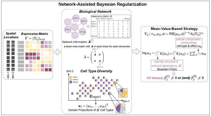
Motivated by the aforementioned challenges, we propose a Bayesian regularization approach for the joint identification of SV genes as shown in Figure 1. Specifically, the ZINB distribution is adopted to account for the count nature, sparsity, and overdispersion of raw expression measurements. The mean-value-based strategy is applied for SV gene detection, which enjoys the advantages of simplicity, interpretability, and computational efficiency. The most substantial advancement is that the proposed approach conducts joint detection with the network dependency structure among genes well incorporated, making it a big step forward from the existing marginal analysis. Moreover, the proposed approach introduces a series of cell-type-specific parameters to effectively correct for the confounding variations induced by varying cell-type compositions across spots. Overall, this study provides a practically useful and biologically meaningful approach for SV gene identification in ST analysis, with improved performance over alternatives as demonstrated in both simulation studies and application to a real-world ST dataset.
2 Methods
Consider a tissue section consisting of spots, genes, and cell types. Let be the ST expression matrix composed of ’s, where is the vector of observed raw counts of the th gene. usually has a very high level of sparsity because of a low capture rate. Each spot is associated with a 2-dimensional coordinate which represents the location of the corresponding spot center.
2.1 Network and Cellular Composition Information for Integration
Consider an undirected network that is constructed using biological information, where is the node set consisting of genes and is the set of edges between nodes. For genes connected within the network, it is expected that they have similar biological functionalities, leading to potentially similar spatial variability, and thus are more likely to be SV or non-SV genes simultaneously. To induce such network-assisted identification, an adjacency matrix is first constructed based on , with if there is an edge between the th and th genes and otherwise, and , for .
As for cellular compositions, denote as the vector of cellular proportions for the th spot, which satisfies the constraint that and . Such information is typically available as ground truth or can be obtained using deconvolution methods such as RCTD (Cable et al., 2022), Redeconve (Zhou et al., 2023), and SONAR (Liu et al., 2023). Since the distributions of cellular proportions usually display spatial relatedness, which may confound SV gene detection, we correct for this potential confounding in SV gene identification.
2.2 Network-assisted Bayesian Modeling
We introduce latent binary variables to accommodate the zero-inflation in and consider the following zero-inflated negative binomial (ZINB) model:
| (1) |
where indicates that is from a Dirac probability measure with a point mass at zero, and otherwise is from a NB distribution with expectation and dispersion . The NB distribution has variance , thus allowing modeling extra variation.
To accommodate spatial differential expression and cell-type-specific confounding, the logarithm of is modeled as:
| (2) |
where is the baseline expression parameter, is the cell-type-specific coefficient to accommodate the potential influence of cellular distributions, and and reflect the degree of spatial differential expression, with being the pre-specified spatialization function to measure the specified trend of spatial gene expression variation.
We adopt the ZINB model due to its superiority for simultaneously accommodating the count measure, over-dispersion, and excessive zeros caused by dropouts. For SV gene identification, significantly different from the previous studies that introduce spatial differential expression via a covariance matrix, which is usually space- and time-consuming and lacks efficiency and scalability for large-scale analysis, we adopt the mean-value-based formulation. The spatial variability is intuitively reflected by and , where the genes with or are regarded as SV. This requires less storage space and also involves a simpler estimation procedure. Moreover, we innovatively utilize a set of cell-type-specific ’s for eliminating the confounding impact of the latent cellular composition, where spots that are spatially closer are often observed to have similar cell-type proportions (Cable et al., 2022). Different from the mean-value-based strategy adopted by Yu and Luo (2022) for marginal cell-type-specific SV gene detection, we focus on the detection of global SV genes while accommodating the cell-type proportion confounding.
2.3 Priors Specification
The proposed priors are defined as follows:
| (3) | ||||
where , represents the effect size of the genes, and denotes the element-wise product. is a vector thresholding function with being a parameter controlling model sparsity and being the adaptive weights. Moreover, is a block diagonal adaptive Laplacian matrix, where with being a rough estimate of and with and with . is a small constant to make strictly positive-definite, which is set as in our numerical work.
The proposed priors have been motivated by the following considerations. The identification of SV genes is achieved using the hard-thresholded Gaussian prior, where is shrunk to zero when (). The thresholded Gaussian prior has been shown as a useful alternative to shrinkage priors in Bayesian sparse analysis (Wu et al., 2024), and is favored here for its simplicity and flexibility as well as its appealing interpretability as a minimal detectable signal. Here, we further introduce a series of weights ’s in to adjust the shrinkage of various ’s to improve selection efficiency, where the genes with strong spatial variability are potentially assigned small weights and thus are more likely to have nonzero ’s.
Moreover, the network dependency is introduced via the graph Laplacian matrix in the covariance matrix of the hard-thresholded Gaussian prior. The proposed network-assisted strategy is motivated by the successes of Laplacian shrinkage in high-dimensional regression analysis (Chakraborty and Lozano, 2019; Cai et al., 2020). Different from these studies, we innovatively conduct SV gene detection with the network structures among genes incorporated. In particular, the Laplacian matrix is further modified with a pre-defined sign matrix to accommodate the scenario where two neighborhood genes are negatively correlated and have opposite directions of spatial variability. With the proposed priors, we have , where for genes and with an edge , the absolute values of and are promoted to be similar, further inducing simultaneous SV or non-SV.
We assign a Bernoulli prior for the latent variable with the hyperparameter , where is the probability that is a dropout zero. A Gamma distribution is assumed for the dispersion parameter . For the variance term , we use the conjugate prior by assigning the Inverse-Gamma distribution . The non-negative uniform prior is assigned for the threshold parameter . For and , the normal priors with mean 0 and variance and are assumed, respectively. These priors have been popular in the existing Bayesian studies.
2.4 Bayesian Inference
The model parameter space consists of , where , and and are the vectors consisting of ’s and ’s, respectively. The posterior distribution is
| (4) | ||||
where denotes the Beta-Bernoulli distribution with the probability mass function .
The posterior sampling is conducted based on the MCMC algorithm. We first introduce the sampling variances and for ’s, ’s, , , and , respectively, and then conduct the following steps at each MCMC iteration, where the symbol “” in the condition position denotes “the rest parameters”.
-
(a)
Sequentially update for with the conditional distribution of given by .
-
(b)
Sequentially sample for , and accept with probability
-
(c)
Sequentially sample for , and accept with probability
-
(d)
Sample from truncated at 0, and accept with probability .
-
(e)
Sample from , where
(5) with being the first derivative of the log-likelihood function with respect to . Then, accept with probability .
-
(f)
Update for and , and update accordingly, where are the index sets of the disconnected sub-networks in .
-
(g)
Sample from with shape parameter and scale parameter .
-
(h)
Sample from truncated at interval , and accept with probability
Here, updating ’s and is achieved through the Gibbs sampler, while the Metropolis-Hasting (MH) algorithm is adopted for sampling ’s, ’s, , and . For sampling , we resort to the preconditioned Crank-Nicolson Langevin dynamics (pCNLD), which takes advantage of the gradient information of the target distribution to speed up convergence. Furthermore, with (5), pCNLD explicitly incorporates the network dependency into the sampling process. The details of the proposed pCNLD sampling are given in Supplementary Section S1. For ’s, since biological networks are often composed of multiple disconnected sub-networks, we propose adopting a set of group-wise weights for the sub-networks for more effectively utilizing network information. Specifically, a series of data-driven weights inversely proportional to the absolute effect sizes of the genes involved in the specific sub-networks are introduced, potentially facilitating the identification of SV genes with weak signals, which may be involved in the sub-networks consisting of SV genes with strong signals and small thresholds. The settings for the hyperparameters and sampling variances are provided in Supplementary Section S2.
For the spatial modeling function , we follow the published studies and consider three most popular functions. Specifically, for which has been transformed to have mean 0 and standard deviation 1, we consider one linear function , two exponential functions and , and two periodic functions and , where and are the 40% and 60% quantiles of , respectively. To accommodate the fact that results may be sensitive to the choice of scale parameter, two values are considered for the exponential and periodic patterns. Then, we conduct the MCMC sampling for each and obtain the estimated posterior expectation , , and , where denotes the samples obtained after burn-in and thinning (we omit the dependence on to simplify notation).
To facilitate the combination of five models, instead of directly considering the values of for SV gene identification, we further introduce a posterior inclusion probability vector estimated as and consider the posterior model probability introduced in Quintana et al. (2011), where denotes the model with . Specifically, for each , we calculate . Here, is the prior probability of model , and we set a non-informative prior with . is the likelihood function with the estimated parameters , and under model . We then utilize ’s as the model-specific weights to obtain the combined . Moreover, as gene with at least one non-zero is identified as SV, we introduce for . Based on ’s, the Bayesian false discovery rate (BFDR) control strategy is adopted for controlling multiplicity. Specifically, with being the desired significance level. We set as 0.05 in our numerical studies. Then, the SV gene set is defined as . To achieve improved stability and better false negative control, in numerical studies, we run five MCMC chains independently, and the genes identified in more than 80% of the chains are finally identified as SV.
To improve computational efficiency, parallelization is implemented with the R package RcppParallel. Specifically, the marginal sequential sampling is divided into parallel programming to reduce computer time. For with the dependency Laplacian matrix incorporated, benefiting from the sparse and block-wise nature of biological networks, the parallelism block-wise sampler is adopted to avoid sampling from a high-dimensional multivariate normal distribution, which further accelerates computation. Take a simulated dataset with and as an example. The average computer time is about 1.01 minutes for 100 iterations on a MacBook Pro with an Intel Core i5 CPU and 16GB RAM.
3 Simulations
3.1 Basic Simulations
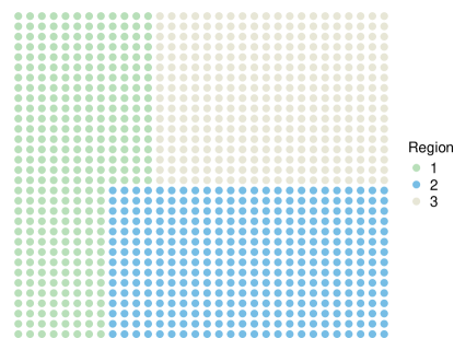
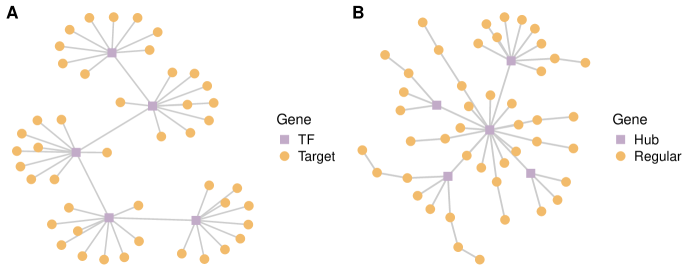
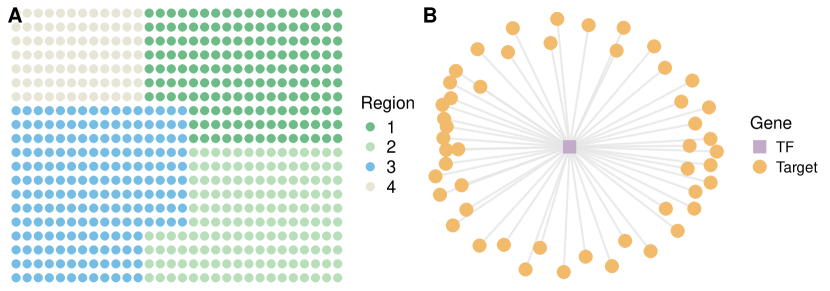
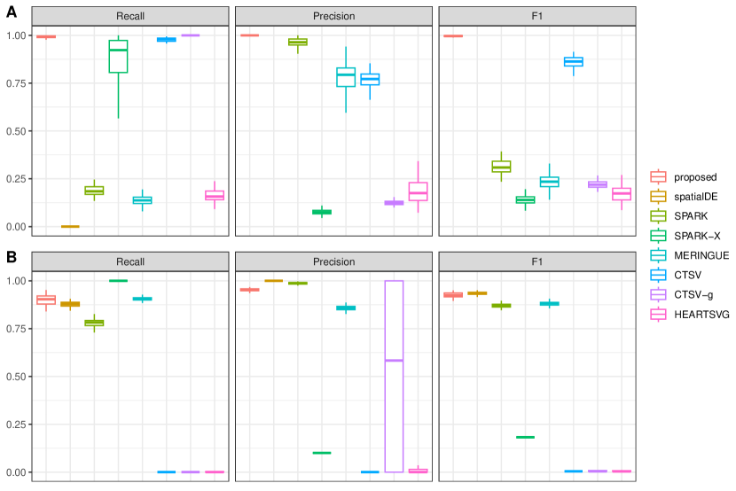
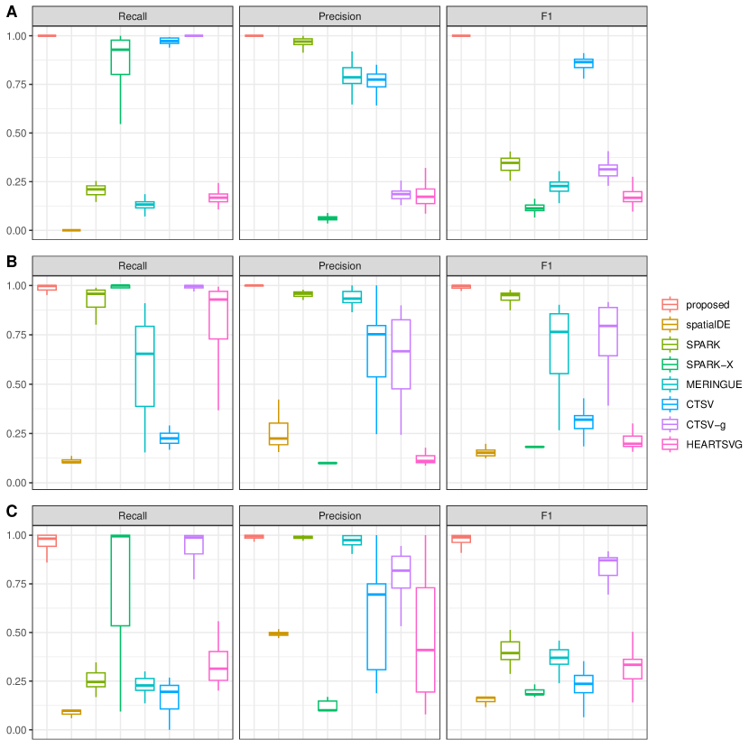
Simulation studies are conducted under the following settings. (a) spots located on a 32 by 32 square lattice, genes, and cell types. (b) The square lattice is partitioned into three regions as displayed in Figure S1, where the cellular compositions ’s are independently sampled from Dirichlet distributions (Region 1), (Region 2), and (Region 3). (c) Consider three types of spatial pattern , including (Linear), (Exponential), and (Periodic). (d) The networks are block-wise and composed of 100 disconnected sub-networks with 50 nodes each. For each sub-network, two types of network structure, namely Star and Scale-free, are considered to mimic the real-world transcription factor regulatory network and interaction network with scale-free properties, respectively. Illustrative examples of the sub-networks are presented in Figure S2(A) and S2(B). (e) All genes in the first ten sub-networks are SV, leading to a total of 500 SV genes. Both positive and negative signals are considered with various levels of magnitude. More detailed settings are provided in Supplementary Section S3.1. (f) The spatial transcriptomics count data is generated from model (1) with the dispersion parameter being 10. Two settings of dropout rates, 0.1 and 0.5, are considered, representing low and high sparsity. The baseline parameter and cell-type-specific effect are independently generated from and , respectively. There are 12 scenarios, comprehensively covering a wide spectrum with different patterns of spatial expressions, different structures of networks and the corresponding spatially variable signals, and different degrees of sparsity.
In addition to the proposed approach, six alternatives are considered: (a) SpatialDE (Svensson et al., 2018), a likelihood ratio test method based on Gaussian process regression, (b) SPARK (Sun et al., 2020), a method based on a Poisson log linear model with a Gaussian process incorporated, (c) SPARK-X (Zhu et al., 2021), a scalable non-parametric test built on a robust covariance test framework, (d) MERINGUE (Miller et al., 2021), a test based on spatial cross-correlation analysis, (e) CTSV and CTSV-g (Yu and Luo, 2022), a test based on the ZINB model for cell-type-specific SV gene identification and global SV gene identification, respectively, and (f) HEARTSVG (Yuan et al., 2023), a distribution-free method that employs the exclusion of non SV genes to infer the presence of SV genes. Among them, SpatialDE, SPARK, CTSV, and CTSV-g are parametric, while SPARK-X, MERINGUE, and HEARTSVG are non-parametric. All the alternatives conduct tests marginally and implement multiple testing control. The implementation details for the competing methods are given in Supplementary Section S3.2.
| Recall | Precision | F1 | Recall | Precision | F1 | |
|---|---|---|---|---|---|---|
| Linear pattern | Star Network | Scale-free Network | ||||
| proposed | 0.992(0.016) | 1.000(0.000) | 0.996(0.008) | 0.991(0.016) | 1.000(0.000) | 0.995(0.008) |
| spatialDE | 0.408(0.172) | 0.990(0.030) | 0.554(0.194) | 0.549(0.183) | 0.990(0.045) | 0.685(0.179) |
| SPARK | 0.907(0.111) | 0.977(0.010) | 0.937(0.065) | 0.911(0.079) | 0.991(0.005) | 0.947(0.046) |
| SPARK-X | 0.887(0.259) | 0.154(0.193) | 0.181(0.021) | 0.772(0.143) | 0.485(0.370) | 0.502(0.287) |
| MERINGUE | 0.562(0.272) | 0.944(0.027) | 0.658(0.241) | 0.642(0.256) | 0.958(0.021) | 0.732(0.219) |
| CTSV | 0.118(0.039) | 0.642(0.249) | 0.186(0.054) | 0.162(0.076) | 0.729(0.193) | 0.249(0.100) |
| CTSV-g | 0.978(0.057) | 0.810(0.104) | 0.880(0.063) | 0.978(0.044) | 0.936(0.013) | 0.956(0.023) |
| HEARTSVG | 0.762(0.246) | 0.284(0.265) | 0.298(0.129) | 0.920(0.142) | 0.178(0.159) | 0.259(0.106) |
| Exponential pattern | Star Network | Scale-free Network | ||||
| proposed | 0.933(0.141) | 1.000(0.001) | 0.959(0.091) | 0.979(0.035) | 1.000(0.001) | 0.989(0.019) |
| spatialDE | 0.036(0.032) | 0.989(0.058) | 0.084(0.053) | 0.278(0.186) | 0.986(0.061) | 0.424(0.232) |
| SPARK | 0.229(0.103) | 0.988(0.013) | 0.360(0.139) | 0.622(0.133) | 0.993(0.005) | 0.756(0.113) |
| SPARK-X | 0.860(0.296) | 0.098(0.004) | 0.177(0.011) | 0.702(0.262) | 0.473(0.369) | 0.442(0.276) |
| MERINGUE | 0.153(0.127) | 0.949(0.042) | 0.248(0.174) | 0.479(0.252) | 0.957(0.023) | 0.592(0.254) |
| CTSV | 0.012(0.022) | 0.116(0.150) | 0.043(0.033) | 0.025(0.034) | 0.366(0.315) | 0.058(0.045) |
| CTSV-g | 0.899(0.173) | 0.918(0.022) | 0.897(0.121) | 0.957(0.078) | 0.934(0.015) | 0.944(0.041) |
| HEARTSVG | 0.282(0.169) | 0.839(0.278) | 0.361(0.195) | 0.634(0.184) | 0.623(0.313) | 0.536(0.188) |
| Periodic pattern | Star Network | Scale-free Network | ||||
| proposed | 0.996(0.008) | 1.000(0.000) | 0.998(0.004) | 0.979(0.130) | 1.000(0.000) | 0.981(0.121) |
| spatialDE | 0.087(0.027) | 0.991(0.053) | 0.158(0.049) | 0.174(0.097) | 0.990(0.056) | 0.286(0.137) |
| SPARK | 0.215(0.088) | 0.987(0.012) | 0.345(0.117) | 0.620(0.130) | 0.992(0.006) | 0.754(0.111) |
| SPARK-X | 0.887(0.268) | 0.156(0.195) | 0.178(0.023) | 0.817(0.238) | 0.492(0.366) | 0.501(0.299) |
| MERINGUE | 0.433(0.265) | 0.952(0.025) | 0.543(0.263) | 0.688(0.277) | 0.961(0.019) | 0.761(0.236) |
| CTSV | 0.088(0.055) | 0.664(0.268) | 0.142(0.072) | 0.215(0.163) | 0.742(0.217) | 0.291(0.187) |
| CTSV-g | 0.969(0.076) | 0.884(0.045) | 0.922(0.042) | 0.990(0.028) | 0.947(0.009) | 0.968(0.015) |
| HEARTSVG | 0.230(0.135) | 0.980(0.043) | 0.355(0.165) | 0.598(0.184) | 0.976(0.084) | 0.720(0.159) |
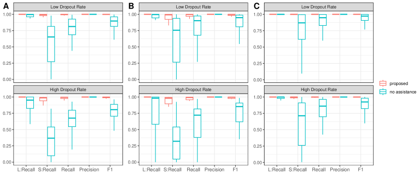
For evaluating identification performance, we adopt Recall = , Precision =, and F1 score = with TP, FP, and FN being the numbers of true positives, false positives, and false negatives, respectively. Under each scenario, we simulate 50 replicates. Summary results under the scenarios with a low dropout rate are given in Table 1. The rest of the results with a high dropout rate are provided in Supplementary Table S1. It is observed that the proposed approach achieves superior accuracy in identifying SV genes with higher F1 scores across all scenarios. Overall, CTSV-g achieves the second-best identification performance since it also accommodates dropouts and over-dispersion through the adoption of ZINB distribution. Improved performance over CTSV-g supports the validity of incorporating network information and accommodating cellular diversity. Furthermore, the majority of the alternatives exhibit good performance with the simple linear patterns while the proposed approach performs stably across different spatial expression patterns. Moreover, similar to those in some published studies, SPARK-X exhibits many false negatives, probably due to its covariance test framework and neglection of cellular composition confounding, and SPARK achieves excellent FP control across all scenarios, mainly attributable to the robust Cauchy combination rule. CTSV identifies the fewest global SV genes across all scenarios due to its concern with cell-type-specific SV genes and inability in accurately identifying genes with global spatial expression variations. Noticeably, under the scenarios with a scale-free network where the signals of the SV genes are larger, all approaches exhibit improved performance with higher F1 score values. However, the superiority of the proposed approach is again evidently observed. With a higher dropout rate, which is more common with practical ST data, all approaches have decayed performance, especially for SpatialDE which is not well-suited for sparse expression distribution. However, the superiority of the proposed approach becomes more prominent.
To better appreciate the operating characteristics of the proposed network-assisted strategy, in Figure S3, we take the scale-free network as an example and further examine the SV genes with large and small signals separately with two Recall indices (L:Recall and S:Recall). Here, besides the proposed approach, we also consider the corresponding approach without the assistance of the network (where is a simple identity matrix). As shown in Figure S3, benefiting from network smoothness, the proposed approach has remarkably improved identification performance, especially for the SV genes with small signals. Such an improvement becomes more obvious for sparser data with a higher dropout rate. Moreover, selection stability is also improved.
3.2 Model Misspecification
We further evaluate performance of the proposed approach under scenarios where the data generation model is misspecified. In particular, we consider two types of model misspecification: (M1) the ZINB model considered in Yu and Luo (2022) where the logarithmic mean value is set as a mix of cell-type-specific expression levels; and (M2) the Poisson model considered in Sun et al. (2020) with the parameters inferred from a real mouse olfactory bulb study. More detailed settings are provided in Supplementary Section S3.4, and summary results are reported in Figure S6.
It is observed that the proposed approach can still maintain its superiority or at least perform comparably to the method that matches the data generation model. Specifically, under model (M1), which favors the CTSV method, the proposed approach achieves more accurate identification with a median F1 equal to 1, while CTSV exhibits the second-best performance. Moreover, even under model (M2) without cellular composition confounding, the proposed approach can still correctly identify SV genes with a median F1 score larger than 0.92. Here, spatialDE and SPARK also behave well since the expression pattern is inferred based on the analysis results of the two approaches.
3.3 Examination on the Noise of Network and Cellular Composition
We continue to examine scenarios with noisy network and cellular composition information. In particular, the noisy network is likely to involve edges that connect both SV and non-SV genes. Two specific generation models are considered, including the ZINB model considered in Section 3.1 with a star network, a linear spatial pattern, and two degrees of sparsity, and the misspecified model (M1) considered in Section 3.2, where in each informative sub-network, about 20% of the genes connected to the TF genes are uninformative. The summary results are reported in Figure S7. It can be seen that the proposed approach can still achieve an effective balance between the prior network information and observation likelihood, leading to certain robustness.
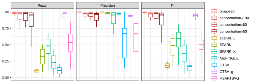
Moreover, to explore the impact of noisy cellular composition on identification performance, we consider the scale-free network with the linear pattern and high sparsity (dropout rate = 0.5), where the cell-type deconvolution estimates are sampled from with being the true value and concentration parameter and 50. The lower value of indicates less accuracy of the cellular composition estimates. The summary results are provided in Figure S8. As expected, the noisy cellular compositions tend to result in decreased identification performance with increased variance. However, even with , the identification performance is still satisfactory, and the superiority over the alternatives maintains.
4 Data Analysis
We apply the proposed approach to the triple-negative breast cancer (TNBC) dataset from a cohort study of TNBC tumors (Bassiouni et al., 2023). A total of 28 tissue sections representing 14 primary TNBC tumors are subject to spatial transcriptomics using the 10x Genomics Visium platform. The raw expression data and the tissue information are available at the Gene Expression Omnibus (GEO) under record GSE210616. Here, we focus on the first tissue section from patient ID 1, which contains 1,109 spots and 36,601 genes. Following the published studies (Charitakis et al., 2023; Yan and Luo, 2024), to improve efficiency and stability, we first remove the genes expressed in fewer than 5 spots and the spots with fewer than 500 expressed genes, resulting in a total of 1,108 spots and 17,781 genes, and then select the top 5,000 highly variable genes for downstream analysis. After preprocessing, the median value of expressed counts across spots is 7,036, and the proportion of zero expressions is about 68.89%.
We consider the protein-protein interaction (PPI) network obtained from the STRING database (Szklarczyk et al., 2023). Integrating the PPI network has been widely adopted in recent breast cancer analysis, which provides a powerful complement for a mechanistic understanding of the genomic alterations related to breast cancer (Kim et al., 2021). In particular, it has been demonstrated in published studies (Pranavathiyani et al., 2019; Chen et al., 2021) that the oncogenes or prognostic genes associated with breast cancer are typically highly interconnected within distinct modules, underscoring the importance of considering the connections within networks in SV gene identification. Matching with this PPI network leads to 1,687 connected genes involved in 164 disconnected sub-networks, while the remaining 3,313 genes are singleton nodes.
For cell-type deconvolution, we adopt the Redeconve algorithm developed in Zhou et al. (2023), which has been proven to have higher accuracy, robustness, and efficacy. More importantly, the superior performance of Redeconve on human breast cancer has been verified based on biological ground truths. To alleviate the impact of rare cell types and to improve interpretability, we follow Yu and Luo (2022) and remove the cell types whose 90 percentile of proportions across spots is less than 0.1, resulting in a total of seven major cell types. The pie charts of the distributions of different cell types across spots are shown in Figure 2(A). It can be seen that most spots consist of cancer and normal epithelial cells, while some spots located at the middle and lower right parts of the tissue section are mostly CAFs.
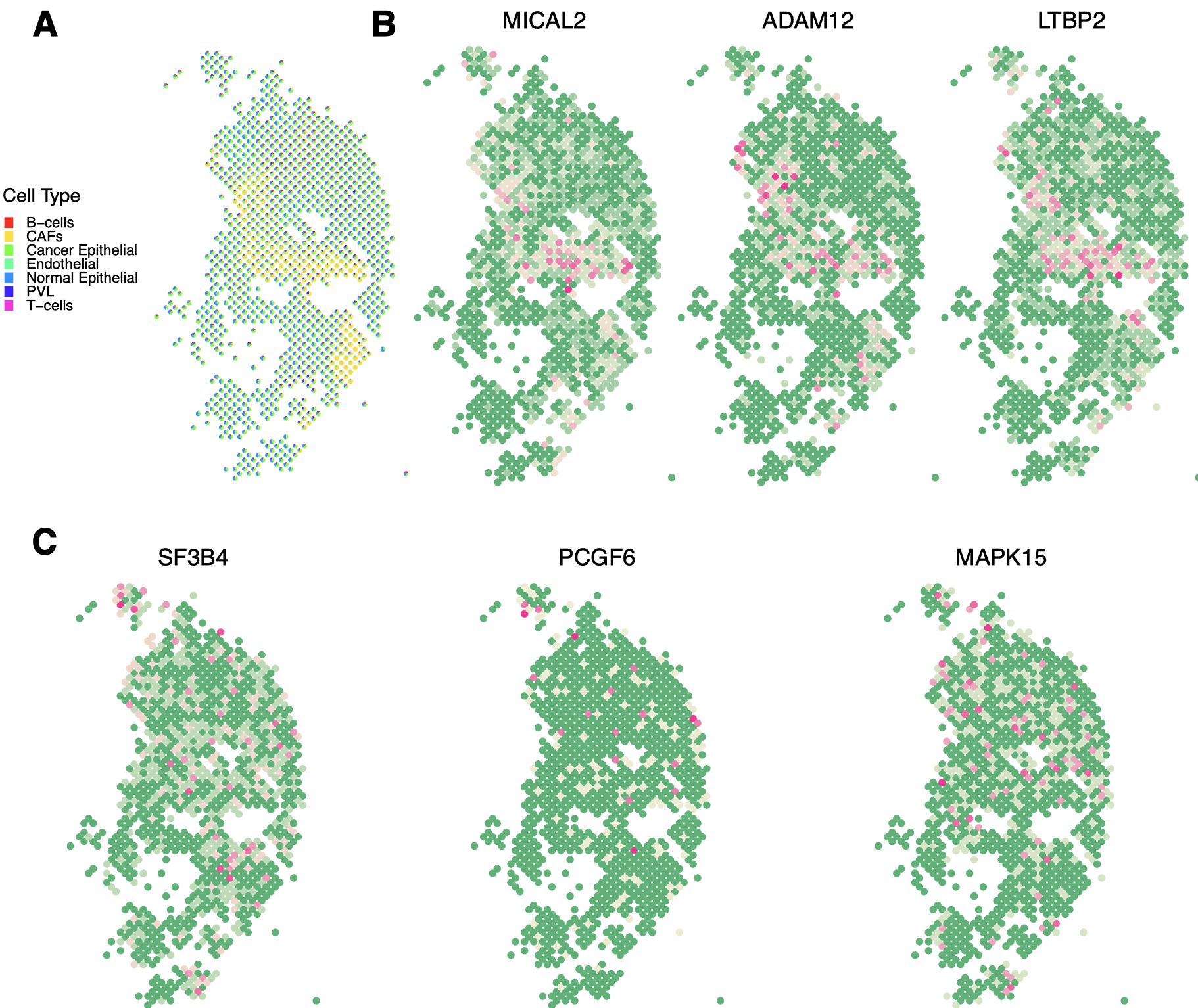
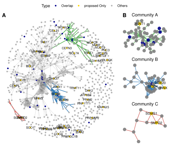
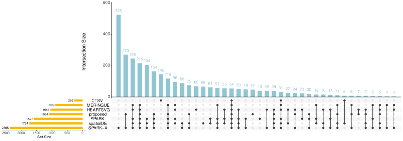
The proposed approach identifies 1,084 SV genes. Among them, 782 are connected in the PPI network, of which the graph representation is shown in Figure 3(A). Analysis is also conducted using the alternatives. The upset plot, which provides the numbers of the SV genes identified by different approaches as well as their overlaps, is shown in Figure 4. Specifically, SPARK-X identifies the largest number of SV genes (2,365), while CTSV detects the smallest (266). A total of 54 overlapping genes are identified by all seven approaches. For SPARK-X, spatialDE, SPARK, HEARTSVG, and MERINGUE, there are more overlapping SV genes (245), mainly due to the potential cell-type diversity confounding that is not well accommodated by these approaches. To provide a more intuitive illustration, among these 245 genes, we take three representative genes MICAL2, ADAM12, and LTBP2 and present their spatial expression patterns in Figure 2(B). All three genes are observed to have significant cell type diversity. Moreover, 47 genes (all connected) are only selected by the proposed approach. Among them, the expression patterns of three representative genes SF3B4, PCGF6, and MAPK15 are presented in Figure 2(C), where clear spatial variability (not driven by cell type diversity) is observed.
To provide additional comparisons for the SV genes identified by different approaches, we obtain the lists of breast cancer driver genes from the Candidate Cancer Gene Database (CCGD), IntOGen, and DriverDB databases, which contain 579, 290, and 222 genes, respectively, and examine whether these genes are identified as SV. The inclusion rates per thousand are (20.30, 11.70, 23.06) for the proposed approach, (13.26, 7.50, 14.42) for spatialDE, (14.58, 7.61, 13.95) for SPARK, (19.45, 5.50, 14.80) for SPARK-X, (0.00, 0.00, 7.52) for CTSV, (12.37, 9.00, 13.50) for MERINGUE, and (12.44, 8.61, 6.70) for HEARTSVG, respectively. This may support the higher power of the proposed approach to some extent.
We then conduct community detection with the 782 connected SV genes and show three representative communities in Figure 3(B), where the overlapping genes identified by all seven approaches (Overlap), genes only identified by the proposed approach (proposed Only), and the remaining genes (Others) are represented by different colors. It is observed that most overlapping genes are hubs with larger values of degrees. Some of the proposed Only genes are connected to the hub genes, for example, SF3B4 and PINX1 in community B, which may exhibit weak spatial patterns but are involved in the same functional organization or regulation mechanism with the hub ones. Some other genes seem to serve as bridge linkage genes with high betweenness centrality. Examples include SGMS2 in community C, which expedites the formulation of the complete gene regulatory networks.
Then, we conduct Gene Ontology (GO) enrichment analysis. Specifically, for the three communities in Figure 3(B), we list the corresponding top five significant GO terms in Table 2, which have important biological implications for breast cancer. For example, in community A, wound healing has been shown to promote the growth of breast cancer, while integrin-mediated signaling has been confirmed to play a significant role in TNBC bone metastasis. The genes involved in community B are mainly enriched in RNA splicing, and the relationships between RNA splicing and a variety of cancers have long been recognized and widely utilized in cancer diagnosis and therapy. For community C, the sphingolipid metabolism has been shown to be essential for breast cancer progression, while ceramide metabolism balance has been confirmed as a critical step of breast cancer development and has been long adopted as a targeted pathway to induce apoptosis in breast cancer cell lines. References that support the above results are presented in Supplementary Section S4.
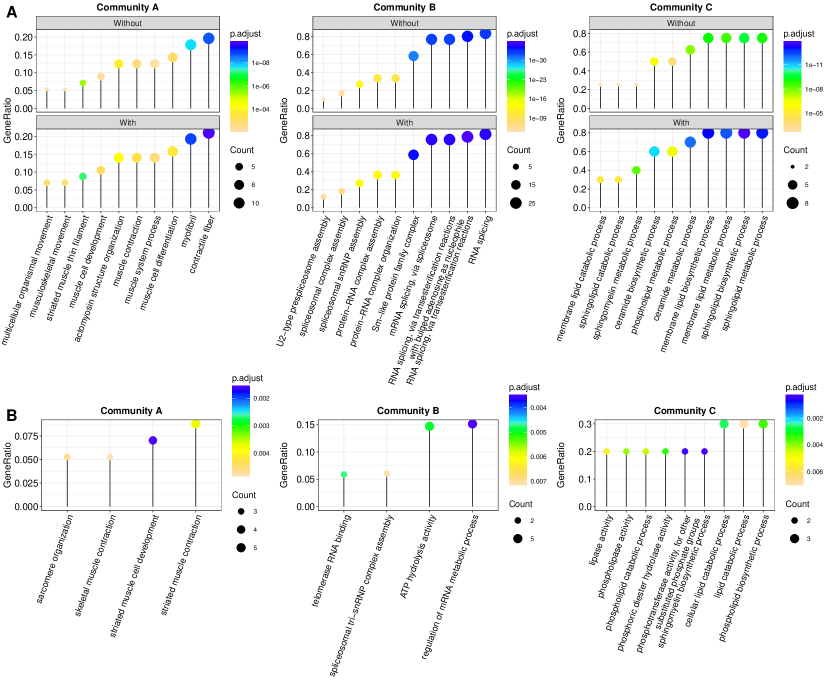
We further take a closer look at the proposed Only genes. Specifically, we conduct GO enrichment analysis for each community again, but with the proposed Only genes eliminated. The comparison results are shown in Figure 5(A), where the top ten significant GO terms with the proposed Only genes included are considered. It can be seen that when the proposed Only genes are included, some more significant GO terms are found. Moreover, the incorporation of the proposed Only genes contributes to some newly detected GO terms (shown in Figure 5(B)), such as skeletal muscle contraction, which has been confirmed to be critical in tumor progression and therapy response (Crist et al., 2022). These evidences suggest the importance of the proposed Only genes in the PPI network and their biological implications.
| ID | adjusted P value | Description | ||
|---|---|---|---|---|
| Community A | ||||
| GO:0042060 | 2.20 | wound healing | ||
| GO:0031589 | 2.20 | cell-substrate adhesion | ||
| GO:0007229 | 3.04 | integrin-mediated signaling pathway | ||
| GO:0007160 | 1.07 | cell-matrix adhesion | ||
| GO:1902905 | 1.07 | positive regulation of supramolecular fiber organization | ||
| Community B | ||||
| GO:0000375 | 1.19 | RNA splicing, via transesterification reactions | ||
| GO:0008380 | 4.22 | RNA splicing | ||
| GO:0000377 | 4.22 |
|
||
| GO:0000398 | 4.22 | mRNA splicing, via spliceosome | ||
| GO:0000387 | 8.16 | spliceosomal snRNP assembly | ||
| Community C | ||||
| GO:0030148 | 1.18 | sphingolipid biosynthetic process | ||
| GO:0046467 | 7.13 | membrane lipid biosynthetic process | ||
| GO:0006665 | 9.42 | sphingolipid metabolic process | ||
| GO:0006643 | 5.62 | membrane lipid metabolic process | ||
| GO:0006672 | 9.39 | ceramide metabolic process | ||
5 Discussion
In this article, we have presented a novel Bayesian regularization approach for the joint identification of SV genes, with the network structure among genes accommodated. The proposed approach has two main advantages. First, attributing to the Bayesian framework, it can automatically incorporate the network structure through the Gaussian Graph Laplacian priors. Compared to most of the existing methods, the utilization of such network information provides more opportunities to search for more biologically sensible SV genes. Second, to tackle the confounding effects of cell type mixtures within spots, cell-type-specific parameters have been introduced to model the variations induced by diverse latent cellular compositions, which are not well accommodated by most existing methods. The extensive simulation studies have revealed that the proposed approach can achieve better performance. The biological implications of the findings from the application to the TNBC dataset have further supported the utility of the proposed approach.
We have considered a series of presupposed spatial patterns and introduced the parametric model. It can be of interest to extend the proposed framework to accommodate unknown spatial patterns using nonparametric functional techniques. The proposed approach has focused on the identification of SV genes. It has the potential to be extended to additionally accommodate region segmentation of the tissue section. In data analysis, we have utilized the PPI information for network construction. Other resources, such as Kyoto Encyclopedia of Genes and Genomes (KEGG) and High-quality INTeractomes (HINT) databases, can also be adopted. Furthermore, a literature search and GO enrichment analysis have demonstrated the significant implications of the findings. A more definitive confirmation from functional validations may be needed.
References
- Arnold et al. (2015) Arnold, K. M., L. M. Opdenaker, D. Flynn, and J. Sims-Mourtada (2015). Wound healing and cancer stem cells: inflammation as a driver of treatment resistance in breast cancer. Cancer Growth and Metastasis 8, CGM–S11286.
- Barrio-Hernandez et al. (2023) Barrio-Hernandez, I., J. Schwartzentruber, A. Shrivastava, N. Del-Toro, A. Gonzalez, Q. Zhang, E. Mountjoy, D. Suveges, D. Ochoa, M. Ghoussaini, et al. (2023). Network expansion of genetic associations defines a pleiotropy map of human cell biology. Nature Genetics 55(3), 389–398.
- Bassiouni et al. (2023) Bassiouni, R., M. O. Idowu, L. D. Gibbs, V. Robila, P. J. Grizzard, M. G. Webb, J. Song, A. Noriega, D. W. Craig, and J. D. Carpten (2023). Spatial transcriptomic analysis of a diverse patient cohort reveals a conserved architecture in triple-negative breast cancer. Cancer Research 83(1), 34–48.
- BinTayyash et al. (2021) BinTayyash, N., S. Georgaka, S. John, S. Ahmed, A. Boukouvalas, J. Hensman, and M. Rattray (2021). Non-parametric modelling of temporal and spatial counts data from rna-seq experiments. Bioinformatics 37(21), 3788–3795.
- Cable et al. (2022) Cable, D. M., E. Murray, L. S. Zou, A. Goeva, E. Z. Macosko, F. Chen, and R. A. Irizarry (2022). Robust decomposition of cell type mixtures in spatial transcriptomics. Nature Biotechnology 40(4), 517–526.
- Cai et al. (2020) Cai, Q., J. Kang, and T. Yu (2020). Bayesian network marker selection via the thresholded graph Laplacian Gaussian prior. Bayesian Analysis 15(1), 79.
- Chakraborty and Lozano (2019) Chakraborty, S. and A. C. Lozano (2019). A graph Laplacian prior for Bayesian variable selection and grouping. Computational Statistics & Data Analysis 136, 72–91.
- Charitakis et al. (2023) Charitakis, N., A. Salim, A. T. Piers, K. I. Watt, E. R. Porrello, D. A. Elliott, and M. Ramialison (2023). Disparities in spatially variable gene calling highlight the need for benchmarking spatial transcriptomics methods. Genome Biology 24(1), 209.
- Chen et al. (2022) Chen, M., C. Wu, Z. Fu, and S. Liu (2022). ICAM1 promotes bone metastasis via integrin-mediated tgf-/emt signaling in triple-negative breast cancer. Cancer Science 113(11), 3751–3765.
- Chen et al. (2021) Chen, Y., F. J. Verbeek, and K. Wolstencroft (2021). Establishing a consensus for the hallmarks of cancer based on gene ontology and pathway annotations. BMC Bioinformatics 22, 1–20.
- Corsetto et al. (2023) Corsetto, P. A., S. Zava, A. M. Rizzo, and I. Colombo (2023). The critical impact of sphingolipid metabolism in breast cancer progression and drug response. International Journal of Molecular Sciences 24(3), 2107.
- Crist et al. (2022) Crist, S. B., T. Nemkov, R. F. Dumpit, J. Dai, S. J. Tapscott, L. D. True, A. Swarbrick, L. B. Sullivan, P. S. Nelson, K. C. Hansen, et al. (2022). Unchecked oxidative stress in skeletal muscle prevents outgrowth of disseminated tumour cells. Nature Cell Biology 24(4), 538–553.
- Elyanow et al. (2020) Elyanow, R., B. Dumitrascu, B. E. Engelhardt, and B. J. Raphael (2020). netNMF-sc: leveraging gene–gene interactions for imputation and dimensionality reduction in single-cell expression analysis. Genome Research 30(2), 195–204.
- García-González et al. (2018) García-González, V., J. F. Díaz-Villanueva, O. Galindo-Hernández, I. Martínez-Navarro, G. Hurtado-Ureta, and A. A. Pérez-Arias (2018). Ceramide metabolism balance, a multifaceted factor in critical steps of breast cancer development. International Journal of Molecular Sciences 19(9), 2527.
- Kim et al. (2021) Kim, M., J. Park, M. Bouhaddou, K. Kim, A. Rojc, M. Modak, M. Soucheray, M. J. McGregor, P. O’Leary, D. Wolf, et al. (2021). A protein interaction landscape of breast cancer. Science 374(6563), eabf3066.
- Li et al. (2021) Li, Q., M. Zhang, Y. Xie, and G. Xiao (2021). Bayesian modeling of spatial molecular profiling data via Gaussian process. Bioinformatics 37(22), 4129–4136.
- Liu et al. (2023) Liu, Z., D. Wu, W. Zhai, and L. Ma (2023). Sonar enables cell type deconvolution with spatially weighted poisson-gamma model for spatial transcriptomics. Nature Communications 14(1), 4727.
- Miller et al. (2021) Miller, B. F., D. Bambah-Mukku, C. Dulac, X. Zhuang, and J. Fan (2021). Characterizing spatial gene expression heterogeneity in spatially resolved single-cell transcriptomic data with nonuniform cellular densities. Genome Research 31(10), 1843–1855.
- Pranavathiyani et al. (2019) Pranavathiyani, G., R. R. Thanmalagan, N. L. Devi, and A. Venkatesan (2019). Integrated transcriptome interactome study of oncogenes and tumor suppressor genes in breast cancer. Genes & Diseases 6(1), 78–87.
- Qin et al. (2023) Qin, X., S. Ma, and M. Wu (2023). Two-level Bayesian interaction analysis for survival data incorporating pathway information. Biometrics 79(3), 1761–1774.
- Quintana et al. (2011) Quintana, M. A., J. L. Berstein, D. C. Thomas, and D. V. Conti (2011). Incorporating model uncertainty in detecting rare variants: the bayesian risk index. Genetic Epidemiology 35(7), 638–649.
- Rao et al. (2021) Rao, A., D. Barkley, G. S. França, and I. Yanai (2021). Exploring tissue architecture using spatial transcriptomics. Nature 596(7871), 211–220.
- Song et al. (2021) Song, Y., X. Zhou, J. Kang, M. T. Aung, M. Zhang, W. Zhao, B. L. Needham, S. L. Kardia, Y. Liu, J. D. Meeker, et al. (2021). Bayesian sparse mediation analysis with targeted penalization of natural indirect effects. Journal of the Royal Statistical Society Series C: Applied Statistics 70(5), 1391–1412.
- Ståhl et al. (2016) Ståhl, P. L., F. Salmén, S. Vickovic, A. Lundmark, J. F. Navarro, J. Magnusson, S. Giacomello, M. Asp, J. O. Westholm, M. Huss, et al. (2016). Visualization and analysis of gene expression in tissue sections by spatial transcriptomics. Science 353(6294), 78–82.
- Stanley and Abdel-Wahab (2022) Stanley, R. F. and O. Abdel-Wahab (2022). Dysregulation and therapeutic targeting of rna splicing in cancer. Nature Cancer 3(5), 536–546.
- Sun et al. (2020) Sun, S., J. Zhu, and X. Zhou (2020). Statistical analysis of spatial expression patterns for spatially resolved transcriptomic studies. Nature Methods 17(2), 193–200.
- Svensson et al. (2018) Svensson, V., S. A. Teichmann, and O. Stegle (2018). SpatialDE: identification of spatially variable genes. Nature Methods 15(5), 343–346.
- Szklarczyk et al. (2023) Szklarczyk, D., R. Kirsch, M. Koutrouli, K. Nastou, F. Mehryary, R. Hachilif, A. L. Gable, T. Fang, N. T. Doncheva, S. Pyysalo, et al. (2023). The STRING database in 2023: protein–protein association networks and functional enrichment analyses for any sequenced genome of interest. Nucleic Acids Research 51(D1), D638–D646.
- Vethakanraj et al. (2015) Vethakanraj, H. S., T. A. Babu, G. B. Sudarsanan, P. K. Duraisamy, and S. A. Kumar (2015). Targeting ceramide metabolic pathway induces apoptosis in human breast cancer cell lines. Biochemical and Biophysical Research Communications 464(3), 833–839.
- Wu et al. (2024) Wu, B., Y. Guo, and J. Kang (2024). Bayesian spatial blind source separation via the thresholded Gaussian process. Journal of the American Statistical Association 119(545), 422–433.
- Yamauchi et al. (2022) Yamauchi, H., K. Nishimura, and A. Yoshimi (2022). Aberrant RNA splicing and therapeutic opportunities in cancers. Cancer Science 113(2), 373–381.
- Yan and Luo (2024) Yan, Y. and X. Luo (2024). Bayesian integrative region segmentation in spatially resolved transcriptomic studies. Journal of the American Statistical Association (just-accepted), 1–21.
- Yu and Luo (2022) Yu, J. and X. Luo (2022). Identification of cell-type-specific spatially variable genes accounting for excess zeros. Bioinformatics 38(17), 4135–4144.
- Yuan et al. (2023) Yuan, X., Y. Ma, R. Gao, S. Cui, B. Fa, Y. Wang, S. Ma, T. Wei, S. S. Ma, and Z. Yu (2023). HEARTSVG: a fast and accurate method for spatially variable gene identification in large-scale spatial transcriptomic data. bioRxiv, 2023–08.
- Zhou et al. (2023) Zhou, Z., Y. Zhong, Z. Zhang, and X. Ren (2023). Spatial transcriptomics deconvolution at single-cell resolution using redeconve. Nature Communications 14(1), 7930.
- Zhu et al. (2021) Zhu, J., S. Sun, and X. Zhou (2021). SPARK-X: non-parametric modeling enables scalable and robust detection of spatial expression patterns for large spatial transcriptomic studies. Genome Biology 22(1), 184.
- Zuo et al. (2024) Zuo, C., J. Xia, and L. Chen (2024). Dissecting tumor microenvironment from spatially resolved transcriptomics data by heterogeneous graph learning. Nature Communications 15(1), 5057.
Supplementary Materials for Joint identification of spatially variable genes via a network-assisted Bayesian regularization approach
S1 Derivation of Step (e) in Posterior Sampling
The preconditioned Crank-Nicolson Langevin dynamics (pCNLD) sampler is adopted for sampling of . The proposed sample of is generated as follows.
with
For the derivative of the hard-thresholding function, a smooth approximation is introduced that for , leading to
where is set as throughout the article.
S2 Detailed Settings for the hyperparameter set
Regarding the hyperparameter set, we assume for a weakly informative prior on . We set and for , and and for . ’s and ’s are set as for all and to yield vague priors for the baseline expression levels and cell-type-specific effects. We set and as the 90% quantile of to help against false positive detection as suggested in Song et al. (2021). The sampling variances and are all adaptively chosen by tuning acceptance rates to 30% in simulation studies and 15% in real data analysis. We perform 2,000 iterations with the first 1000 discarded as burn-in and thinning by 10 in the simulations, and 3,000 iterations with the first 2000 burn-in and thinning by 10 in the data analysis.
S3 Additional simulation settings and results
S3.1 Detailed Settings for Basic Simulations
Detailed settings for the spatial effects:
-
(a)
Star network
For each informative sub-network, the transcription factor (TF) gene and its connected target genes have the same sign of spatial effect (either all positive or all negative), while the magnitudes satisfy that with being the number of the target genes regulated by TF. Specifically, the values of and are fixed as and for all three patterns, while and for linear pattern, and for periodic pattern, and and for exponential pattern.
For the non-informative sub-networks, .
-
(b)
Scale-free network
For each informative sub-network, the spatial effects of the hub gene and its connected regular genes are randomly assigned as positive or negative. In addition, the magnitudes of are simulated from for all three patterns. For the magnitudes of the regular SV genes, consider two types with large and small signal strengths, respectively. Specifically, for both , the magnitudes are simulated as follows: for linear pattern, for periodic pattern, and for exponential pattern, where and 2 for small and large strengths, respectively.
For the non-informative sub-networks, .
S3.2 Implementation Details of the Competing Methods
-
(a)
SpatialDE: The source code for SpatialDE is publicly available on https://github.com/Teichlab/SpatialDE. Following the instructions, we filter the practically unobserved genes with total observations less than 3. The linear regression is conducted on the raw count matrix to account for the potential bias caused by library size or sequencing depth. The main function for SV gene detection is SpatialDE.run() with the arguments being the coordinate information and the sample residual expressions corrected by the linear regression. To account for multiple testing, the genes with qval less than 0.05 are identified as SV.
-
(b)
SPARK: The source code for SPARK is publicly available on https://github.com/xzhoulab/SPARK. Following the instructions, we filter genes that are expressed in less than 10% spots and spots with the total observations less than 10. The statistical model under the null hypothesis is first fit by employing the function spark.vc(), and the function spark.test() is subsequently employed for SV gene detection. Then, the genes with adjusted_pvalue less than 0.05 are identified as SV.
-
(c)
SPARK-X: The source code for SPARK-X is publicly available on https://github.com/xzhoulab/SPARK. The SV gene detection is implemented with the main function sparkx() where the argument option is set as “mixture” for multiple kernels testing. To account for the impact of latent cellular compositions, as conducted in the original paper, each spot is assigned its major cell type, with the argument X_in being the matrix of binary indicators. Then, the genes with adjustedPval less than 0.05 are identified as SV.
-
(d)
MERINGUE: The source code for MERINGUE is publicly available on https://github.com/JEFworks-Lab/MERINGUE. The non-expressed genes and spots are filtered following the tutorial. Normalization is conducted for the raw count matrix by employing the function normalizeCounts(). For SV gene detection, the neighborhood relationships are first constructed using the function getSpatialNeighbors() with the argument filterDist set as the default value 2.5. Then, the SV genes are identified with the function filterSpatialPatterns() with the arguments minPercentCells set as 0.05 to restrict that the SV genes are driven by more than 5% of spots. The adjusted significance threshold is set as 0.05 through setting the arguments adjustPv as TRUE and alpha as 0.05.
-
(e)
CTSV and CTSV-g: The source code for CTSV is publicly available on https://github.com/jingeyu/CTSV. The SV gene detection is conducted through the main function ctsv(). Specifically, the cell-type-specific SV genes are identified with the argument being the matrix composed of ’s (). The final SV gene set is the union of all cell-type-specific SV genes. We also conduct the global SV gene detection without accommodation for the cellular composition in the simulation studies (CTSV-g). Specifically, the argument is set as . For both CTSV and CTSV-g, the SV genes are identified through function svGene() with the significance threshold thre.alpha set as 0.05.
-
(f)
HEARTSVG: The source code for HEARTSVG is publicly available on https://github.com/cz0316/HEARTSVG. The detection of SV genes is conducted through the main function heartsvg() with the raw count matrix first scaled as recommended. The Holm method is further conducted for multiple testing control. The genes with adjusted P values p_adj less than 0.05 are identified as SV.
S3.3 Additional Simulation Results under the Scenarios with a High Dropout Rate
| Recall | Precision | F1 | Recall | Precision | F1 | |
|---|---|---|---|---|---|---|
| Linear pattern | Star Network | Scale-free Network | ||||
| proposed | 0.975(0.081) | 1.000(0.000) | 0.985(0.053) | 0.965(0.106) | 1.000(0.000) | 0.978(0.078) |
| spatialDE | 0.079(0.036) | 0.999(0.004) | 0.168(0.028) | 0.093(0.039) | 1.000(0.000) | 0.174(0.060) |
| SPARK | 0.169(0.065) | 0.985(0.013) | 0.284(0.094) | 0.312(0.135) | 0.983(0.016) | 0.457(0.163) |
| SPARK-X | 0.735(0.361) | 0.220(0.276) | 0.179(0.025) | 0.465(0.158) | 0.847(0.226) | 0.567(0.171) |
| MERINGUE | 0.133(0.044) | 0.967(0.026) | 0.230(0.069) | 0.238(0.111) | 0.974(0.022) | 0.369(0.145) |
| CTSV | 0.085(0.051) | 0.551(0.293) | 0.128(0.059) | 0.103(0.060) | 0.571(0.267) | 0.147(0.073) |
| CTSV-g | 0.921(0.131) | 0.883(0.039) | 0.894(0.074) | 0.932(0.100) | 0.939(0.015) | 0.932(0.055) |
| HEARTSVG | 0.205(0.079) | 0.674(0.261) | 0.284(0.075) | 0.534(0.178) | 0.616(0.258) | 0.494(0.114) |
| Exponential pattern | Star Network | Scale-free Network | ||||
| proposed | 0.873(0.215) | 1.000(0.000) | 0.913(0.170) | 0.937(0.152) | 1.000(0.001) | 0.958(0.128) |
| spatialDE | 0.000(0.000) | -(-) | -(-) | 0.000(0.000) | -(-) | -(-) |
| SPARK | 0.001(0.002) | 0.897(0.285) | 0.007(0.003) | 0.009(0.009) | 0.965(0.098) | 0.024(0.015) |
| SPARK-X | 0.698(0.394) | 0.131(0.157) | 0.165(0.041) | 0.211(0.181) | 0.820(0.263) | 0.319(0.224) |
| MERINGUE | 0.004(0.005) | 0.900(0.251) | 0.013(0.011) | 0.038(0.035) | 0.899(0.173) | 0.082(0.061) |
| CTSV | 0.018(0.029) | 0.103(0.129) | 0.044(0.032) | 0.023(0.032) | 0.250(0.035) | 0.043(0.036) |
| CTSV-g | 0.733(0.278) | 0.929(0.018) | 0.783(0.215) | 0.878(0.154) | 0.937(0.013) | 0.898(0.095) |
| HEARTSVG | 0.029(0.020) | 0.890(0.186) | 0.057(0.036) | 0.193(0.112) | 0.933(0.094) | 0.304(0.154) |
| Periodic pattern | Star Network | Scale-free Network | ||||
| proposed | 0.983(0.099) | 1.000(0.000) | 0.988(0.076) | 0.977(0.134) | 1.000(0.000) | 0.980(0.127) |
| spatialDE | 0.000(0.000) | -(-) | -(-) | 0.001(0.002) | 1.000(0.000) | 0.006(0.004) |
| SPARK | 0.029(0.026) | 0.954(0.177) | 0.070(0.043) | 0.050(0.037) | 0.975(0.038) | 0.112(0.056) |
| SPARK-X | 0.723(0.370) | 0.213(0.267) | 0.173(0.033) | 0.437(0.222) | 0.845(0.236) | 0.531(0.246) |
| MERINGUE | 0.092(0.033) | 0.965(0.035) | 0.166(0.057) | 0.272(0.149) | 0.972(0.024) | 0.401(0.189) |
| CTSV | 0.061(0.062) | 0.442(0.315) | 0.094(0.074) | 0.098(0.092) | 0.565(0.302) | 0.152(0.114) |
| CTSV-g | 0.890(0.166) | 0.912(0.024) | 0.889(0.106) | 0.959(0.080) | 0.945(0.010) | 0.950(0.044) |
| HEARTSVG | 0.075(0.017) | 0.988(0.021) | 0.139(0.029) | 0.159(0.055) | 0.994(0.010) | 0.270(0.083) |
S3.4 Simulations under Model Misspecification
We considered two types of model misspecification scenarios as follows.
-
(M1)
ZINB model considered in Yu and Luo (2022). Specifically, the raw count data is generated from where with . Following Yu and Luo (2022), consider spots located on a grid and partitioned into four regions as shown in Figure S3.4(A). Consider underlying cell types where the cellular composition of spots in regions 1, 2, 3, and 4 are independently sampled from , , , and , respectively. Consider genes, involving in a block-wise network composed of 100 disconnected sub-networks with 50 nodes each. Here, each sub-network includes one TF gene and 49 connected target genes, as shown in Figure S3.4(B). All genes in the first seven sub-networks are SV. Specifically, the th to th genes are set as cell-type- SV for , resulting in a total of 350 SV genes. The spatial effect function is fixed as a linear pattern with and for SV genes and = = 0 for non-SV genes. For , first simulate from for , and then simulate 150 differentially expressed genes for each cell type from independently, where and . In addition, and ’s are simulated from a Bernoulli distribution .
-
(M2)
Poisson model considered in Sun et al. (2020). The raw count data is generated as , where with and being the intercept and residual error term, respectively. Specifically, following Sun et al. (2020), consider 260 spots collected in the mouse olfactory bulb study (Ståhl et al., 2016) with the corresponding parameters inferred from the data analysis conducted by spatialDE and SPARK, and genes. The network is set as the same as (M1) (as shown in Figure S3.4(B)), except that all genes in the first ten sub-networks are SV, resulting in a total number of 500 SV genes. For non-SV genes, is set to be across all spots, which corresponds to the median of the intercept estimates in the mouse olfactory data analysis. For SV genes, the spots are categorized into two groups, including the group with low expression levels (green) and the group with high expression levels (pink), according to the spatial patterns of the identified SV genes in the mouse olfactory bulb data, as illustrated in Figure S3.5. In particular, ’s for the low group are set as while ’s for the high group are set as and for the target and TF genes, respectively, according to the estimates for mean values. ’s are independently simulated from , which is approximately the first quantile of the non-spatial variance estimates. For cellular composition variations, consider underlying cell types, where ’s of spots from high and low groups are independently sampled from and , respectively. is set as 0 for , so that the cellular composition variations do not contribute to the expression levels. ’s are obtained based on the real counts.

S4 References that support the biological implications of three communities
In community A, wound healing has been shown to promote the growth of breast cancer (Arnold et al., 2015), while integrin-mediated signaling has been confirmed to play a significant role in TNBC bone metastasis (Chen et al., 2022). The genes involved in community B are mainly enriched in RNA splicing, and the relationships between RNA splicing and a variety of cancers have long been recognized and widely utilized in cancer diagnosis and therapy (Stanley and Abdel-Wahab, 2022; Yamauchi et al., 2022). For community C, the sphingolipid metabolism has been shown to be essential for breast cancer progression (Corsetto et al., 2023), while ceramide metabolism balance has been confirmed as a critical step of breast cancer development (García-González et al., 2018) and has been long adopted as a targeted pathway to induce apoptosis in breast cancer cell lines (Vethakanraj et al., 2015).