This paper was converted on www.awesomepapers.org from LaTeX by an anonymous user.
Want to know more? Visit the Converter page.

Joint Learning of Linear Time-Invariant Dynamical Systems

Aditya Modi admodi@umich.edu    Mohamad Kazem Shirani Faradonbeh mkshiranyf@gmail.com    Ambuj Tewari tewaria@umich.edu    George Michailidis gmichail@ucla.edu Microsoft, Mountain View, CA-94043, USA Department of Mathematics, Southern Methodist University, Dallas, TX-75275, USA Department of Statistics, University of Michigan, Ann Arbor, MI-48109, USA Department of Statistics, University of California, Los Angeles, CA-90095, USA
Abstract

Linear time-invariant systems are very popular models in system theory and applications. A fundamental problem in system identification that remains rather unaddressed in extant literature is to leverage commonalities amongst related systems to estimate their transition matrices more accurately. To address this problem, we investigate methods for jointly estimating the transition matrices of multiple systems. It is assumed that the transition matrices are unknown linear functions of some unknown shared basis matrices. We establish finite-time estimation error rates that fully reflect the roles of trajectory lengths, dimension, and number of systems under consideration. The presented results are fairly general and show the significant gains that can be achieved by pooling data across systems, in comparison to learning each system individually. Further, they are shown to be robust against moderate model misspecifications. To obtain the results, we develop novel techniques that are of independent interest and are applicable to similar problems. They include tightly bounding estimation errors in terms of the eigen-structures of transition matrices, establishing sharp high probability bounds for singular values of dependent random matrices, and capturing effects of misspecified transition matrices as the systems evolve over time.

keywords:
Multiple Linear Systems; Data Sharing; Finite Time Identification; Autoregressive Processes; Joint Estimation.
thanks: This paper was not presented at any IFAC meeting.

, , ,

1 Introduction

The problem of identifying the transition matrices in linear time-invariant (LTI) systems has been extensively studied in the literature [8, 26, 29]. Recent papers establish finite-time rates for accurately learning the dynamics in various online and offline settings [16, 36, 39]. Notably, existing results are established when the goal is to identify the transition matrix of a single system.

However, in many application areas of LTI systems, one observes state trajectories of multiple dynamical systems. So, in order to be able to efficiently use the full data of all state trajectories and utilize the possible commonalities the systems share, we need to estimate the transition matrices of all systems jointly. The range of applications is remarkably extensive, including dynamics of economic indicators in US states [35, 40, 42], flight dynamics of airplanes at different altitudes [6], drivers of gene expressions across related species [5, 19], time series data of multiple subjects that suffer from the same disease [38, 41], and commonalities among multiple subsystems in control engineering [43].

In all these settings, there are strong similarities in the dynamics of the systems, which are unknown and need to be learned from the data. Hence, it becomes of interest to develop a joint learning strategy for the system parameters, by pooling the data of the underlying systems together and learn the unknown similarities in their dynamics. In particular, this strategy is of extra importance in settings wherein the available data is limited, for example when the state trajectories are short or the dimensions are not small.

In general, joint learning (also referred to as multitask learning) approaches aim to study estimation methods subject to unknown similarities across the data generation mechanisms. Joint learning methods are studied in supervised learning and online settings [10, 4, 32, 33, 3]. Their theoretical analyses are obtained rely on a number of technical assumptions regarding the data, including independence, identical distributions, boundedness, richness, and isotropy.

However, for the problem of joint learning of dynamical systems, additional technical challenges are present. First, the observations are temporally dependent. Second, the number of unknown parameters is the square of the dimension of the system, which impacts the learning accuracy. Third, since in many applications the dynamics matrices of the underlying LTI systems might possess eigenvalues of (almost) unit magnitude, conventional approaches for dependent data (e.g., mixing) inapplicable [16, 36, 39]. Fourth, the spectral properties of the transition matrices play a critical role on the magnitude of the estimation errors. Technically, the state vectors of the systems can scale exponentially with the multiplicities of the eigenvalues of the transition matrices (which can be as large as the dimension). Accordingly, novel techniques are required for considering all important factors and new analytical tools are needed for establishing useful rates for estimation error. Further details and technical discussions are provided in Section 3.

We focus on a commonly used setting for joint learning that involves two layers of uncertainties. It lets all systems share a common basis, while coefficients of the linear combinations are idiosyncratic for each system. Such settings are adopted in multitask regression, linear bandits, and Markov decision processes [14, 22, 31, 44]. From another point of view, this assumption that the system transition matrices are unknown linear combinations of unknown basis matrices can be considered as a first-order approximation for unknown non-linear dynamical systems [27, 30]. Further, these compound layers of uncertainties subsume a recently studied case for mixtures of LTI systems where under additional assumptions such as exponential stability and distinguishable transition matrices, joint learning from unlabeled state trajectories outperforms individual system identification [11].

The main contributions of this work can be summarized as follows. We provide novel finite-time estimation error bounds for jointly learning multiple systems, and establish that pooling the data of state trajectories can drastically decrease the estimation error. Our analysis also presents effects of different parameters on estimation accuracy, including dimension, spectral radius, eigenvalues multiplicity, tail properties of the noise processes, and heterogeneity among the systems. Further, we study learning accuracy in the presence of model misspecifications and show that the developed joint estimator can robustly handle moderate violations of the shared structure in the dynamics matrices.

In order to obtain the results, we employ advanced techniques from random matrix theory and prove sharp concentration results for sums of multiple dependent random matrices. Then, we establish tight and simultaneous high-probability confidence bounds for the sample covariance matrices of the systems under study. The analyses precisely characterize the dependence of the presented bounds on the spectral properties of the transition matrices, condition numbers, and block-sizes in the Jordan decomposition. Further, to address the issue of temporal dependence, we extend self-normalized martingale bounds to multiple matrix-valued martingales, subject to shared structures across the systems. We also present a robustness result by showing that the error due to misspecifications can be effectively controlled.

The remainder of the paper is organized as follows. The problem is formulated in Section 2. In Section 3, we describe the joint-learning procedure, study the per-system estimation error, and provide the roles of various key quantities. Then, investigation of robustness to model misspecification and the impact of violating the shared structure are discussed in Section 4. We provide numerical illustrations for joint learning in Section 5 and present the proofs of our results in the subsequent sections. Finally, the paper is concluded in Section 10.

Notation. For a matrix AA, AA^{\prime} denotes the transpose of AA. For square matrices, we use the following order of eigenvalues in terms of their magnitudes: |λmax(A)|=|λ1(A)||λ2(A)||λd(A)|=|λmin(A)|\left|\lambda_{\max}(A)\right|=\left|\lambda_{1}(A)\right|\geq\left|\lambda_{2}(A)\right|\geq\cdots\geq\left|\lambda_{d}(A)\right|=\left|\lambda_{\min}(A)\right|. For singular values, we employ σmin(A)\sigma_{\min}(A) and σmax(A)\sigma_{\max}(A). For any vector vdv\in\mathbb{C}^{d}, let vp{\left|\kern-1.29167pt\left|v\right|\kern-1.29167pt\right|}_{p} denote its p\ell_{p} norm. We use ||||||γβ{\left|\kern-1.29167pt\left|\kern-1.29167pt\left|\cdot\right|\kern-1.29167pt\right|\kern-1.29167pt\right|}_{\gamma\rightarrow\beta} to denote the matrix operator-norm for β,γ[1,]\beta,\gamma\in[1,\infty] and Ad1×d2A\in\mathbb{C}^{d_{1}\times d_{2}}: |A|γβ=supv𝟎Avβ/vγ\left|\!\left|\!\left|A\right|\!\right|\!\right|_{{\gamma\rightarrow\beta}}=\sup\limits_{v\neq{\bf 0}}{{\left|\kern-1.29167pt\left|Av\right|\kern-1.29167pt\right|}_{\beta}}/{{\left|\kern-1.29167pt\left|v\right|\kern-1.29167pt\right|}_{\gamma}}. When γ=β\gamma=\beta, we simply write |A|β{\left|\kern-1.29167pt\left|\kern-1.29167pt\left|A\right|\kern-1.29167pt\right|\kern-1.29167pt\right|}_{\beta}. For functions f,g:𝒳f,g:\mathcal{X}\rightarrow\mathbb{R}, we write fgf\lesssim g, if f(x)cg(x)f(x)\leq cg(x) for a universal constant c>0c>0. Similarly, we use f=O(g)f=O(g) and f=Ω(h)f=\Omega(h), if 0f(n)c1g(n)0\leq f(n)\leq c_{1}g(n) for all nn1n\geq n_{1}, and 0c2h(n)f(n)0\leq c_{2}h(n)\leq f(n) for all nn2n\geq n_{2}, respectively, where c1,c2,n1,n2c_{1},c_{2},n_{1},n_{2} are large enough constants. For any two matrices of the same dimensions, we define the inner product A,B=tr(AB)\left\langle A,B\right\rangle=\mathop{\mathrm{tr}}\left(A^{\prime}B\right). Then, the Frobenius norm becomes AF=A,A{\left|\kern-1.29167pt\left|A\right|\kern-1.29167pt\right|}_{F}=\sqrt{\left\langle A,A\right\rangle}. The sigma-field generated by X1,X2,,XnX_{1},X_{2},\ldots,X_{n} is denoted by σ(X1,X2,Xn)\sigma(X_{1},X_{2},\ldots X_{n}). We denote the ii-th component of the vector xdx\in\mathbb{R}^{d} by x[i]x[i]. Finally, for nn\in\mathbb{N}, the shorthand [n][n] is the set {1,2,,n}\left\{1,2,\ldots,n\right\}.

2 Problem Formulation

Refer to caption
(a) |λ1(A)|<1\left|\lambda_{1}(A)\right|<1
Refer to caption
(b) |λ1(A)|1\left|\lambda_{1}(A)\right|\approx 1
Figure 1: Logarithm of the magnitude of the state vectors vs. time, for different block-sizes in the Jordan forms of the transition matrices, which is denoted by ll in (4). The exponential scaling of the state vectors with ll can be seen in both plots.

Our main goal is to study the rates of jointly learning dynamics of multiple LTI systems. Data consists of state trajectories of length TT from MM different systems. Specifically, for m[M]m\in[M] and t=0,1,,Tt=0,1,\ldots,T, let xm(t)dx_{m}(t)\in\mathbb{R}^{d} denote the state of the mm-th system, that evolves according to the Vector Auto-Regressive (VAR) process

xm(t+1)=Amxm(t)+ηm(t+1).\displaystyle x_{m}(t+1)=A_{m}x_{m}(t)+\eta_{m}(t+1). (1)

Above, Amd×dA_{m}\in\mathbb{R}^{d\times d} denotes the true unknown transition matrix of the mm-th system and ηm(t+1)\eta_{m}(t+1) is a mean zero noise. For succinctness, we use Θ\Theta^{*} to denote the set of all MM transition matrices {Am}m=1M\{A_{m}\}_{m=1}^{M}. The transition matrices are related as will be specified in Assumption 3.

Note that the above setting includes systems with longer memories. Indeed, if the states x~m(t)d~\tilde{x}_{m}(t)\in\mathbb{R}^{\tilde{d}} obey

x~m(t)=Bm,1x~m(t1)++Bm,qx~m(tq)+ηm(t),\tilde{x}_{m}(t)=B_{m,1}\tilde{x}_{m}(t-1)+\cdots+B_{m,q}\tilde{x}_{m}(t-q)+\eta_{m}(t),

then, by concatenating x~m(t1),,x~m(tq)\tilde{x}_{m}(t-1),\cdots,\tilde{x}_{m}(t-q) in one larger vector xm(t1)x_{m}(t-1), the new state dynamics is (1), for d=qd~d=q\tilde{d} and Am=[Bm,1Bm,q1Bm,qI(q1)d~0].A_{m}=\begin{bmatrix}B_{m,1}\cdots B_{m,q-1}&B_{m,q}\\ I_{(q-1)\tilde{d}}&0\end{bmatrix}.

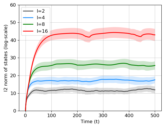
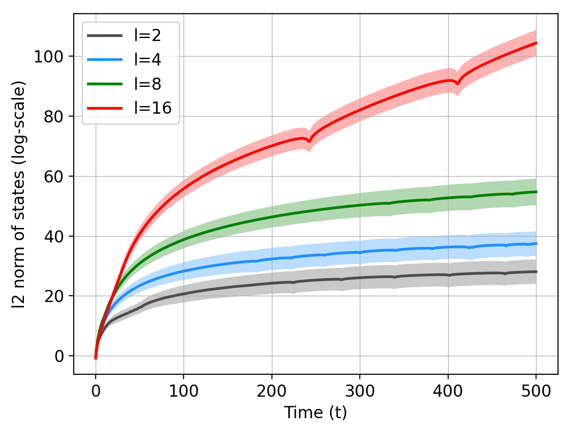
We assume that the system states do not explode in the sense that the spectral radius of the transition matrix AmA_{m} can be slightly larger than one. This is required for the systems to be able to operate for a reasonable time length [25, 15]. Note that this assumption still lets the state vectors grow with time, as shown in Figure 1.

Assumption 1.

For all m[M]m\in[M], we have |λ1(Am)|1+ρ/T\left|\lambda_{1}(A_{m})\right|\leq 1+\rho/T, where ρ>0\rho>0 is a fixed constant.

In addition to the magnitudes of the eigenvalues, further properties of the transition matrices heavily determine the temporal evolution of the systems. A very important one is the size of the largest block in the Jordan decomposition of AmA_{m}, which will be rigorously defined shortly. This quantity is denoted by ll in (4). The impact of ll on the state trajectories is illustrated in Figure 1, wherein we plot the logarithm of the magnitude of state vectors for linear systems of dimension d=32d=32. The upper plot depicts state magnitude for stable systems and for blocks of the size l=2,4,8,16l=2,4,8,16 in the Jordan decomposition of the transition matrices. It illustrates that the state vector scales exponentially with ll. Note that ll can be as large as the system dimension dd.

Moreover, the case of transition matrices with eigenvalues close to (or exactly on) the unit circle is provided in the lower panel in Figure 1. It illustrates that the state vectors grow polynomially with time, whereas the scaling with the block-size ll is exponential. Therefore, in design and analysis of joint learning methods, one needs to carefully consider the effects of ll and |λ1(Am)|\left|\lambda_{1}(A_{m})\right|.

Next, we express the probabilistic properties of the stochastic processes driving the dynamical systems. Let t=σ(x1:M(0),η1:M(1),,η1:M(t))\mathcal{F}_{t}=\sigma(x_{1:M}(0),\eta_{1:M}(1),\dots,\eta_{1:M}(t)) denote the filtration generated by the the initial state and the sequence of noise vectors. Based on this, we adopt the following ubiquitous setting that lets the noise process {ηm(t)}t=1\{\eta_{m}(t)\}_{t=1}^{\infty} be a sub-Gaussian martingale difference sequence. Note that by definition, ηm(t)\eta_{m}(t) is t\mathcal{F}_{t}-measurable.

Assumption 2.

For all systems m[M]m\in[M], we have 𝔼[ηm(t)|t1]=𝟎\mathbb{E}\left[\eta_{m}(t)|\mathcal{F}_{t-1}\right]={\bf 0} and 𝔼[ηm(t)ηm(t)|t1]=C\mathbb{E}\left[\eta_{m}(t)\eta_{m}(t)^{\prime}|\mathcal{F}_{t-1}\right]=C. Further, ηm(t)\eta_{m}(t) is sub-Gaussian; for all λd\lambda\in\mathbb{R}^{d}:

𝔼[expλ,ηm(t)|t1]exp(λ2σ2/2).\mathbb{E}\left[\exp\left\langle\lambda,\eta_{m}(t)\right\rangle|\mathcal{F}_{t-1}\right]\leq\exp\left({\left|\kern-1.29167pt\left|\lambda\right|\kern-1.29167pt\right|}^{2}\sigma^{2}/2\right).

Henceforth, we denote c2=max(σ2,λmax(C))c^{2}=\max(\sigma^{2},\lambda_{\max}(C)).

The above assumption is widely-used in the finite-sample analysis of statistical learning methods [1, 17]. It includes normally distributed martingale difference sequences, for which Assumption 2 is satisfied with σ2=λmax(C)\sigma^{2}=\lambda_{\max}(C). Moreover, if the coordinates of ηm(t)\eta_{m}(t) are (conditionally) independent and have sub-Gaussian distributions with constant σi\sigma_{i}, it suffices to let σ2=i=1dσi2\sigma^{2}=\sum_{i=1}^{d}\sigma_{i}^{2}. We let a common noise covariance matrix for the ease of expression. However, the results simply generalize to covariance matrices that vary with time and across the systems, by appropriately replacing upper- and lower-bounds of the matrices [16, 36, 39].

For a single system m[M]m\in[M], its underlying transition matrices AmA_{m} can be individually learned from its own state trajectory data by using the least squares estimator [16, 36]. We are interested in jointly learning the transition matrices of all MM systems under the assumption that they share the following common structure.

Assumption 3 (Shared Basis).

Each transition matrix AmA_{m} can be expressed as

Am=i=1kβm[i]Wi,\displaystyle A_{m}=\sum_{i=1}^{k}\beta^{*}_{m}[i]W^{*}_{i}, (2)

where {Wi}i=1k\{W^{*}_{i}\}_{i=1}^{k} are common d×d{d\times d} matrices and βmk\beta^{*}_{m}\in\mathbb{R}^{k} contains the idiosyncratic coefficients for system mm.

This assumption is commonly-used in the literature of jointly learning multiple parameters [14, 44]. Intuitively, it states that each system evolves by combining the effects of kk systems. These kk unknown systems behind the scene are shared by all systems m[M]m\in[M], the weight of each of which is reflected by the idiosyncratic coefficients that are collected in βm\beta^{*}_{m} for system mm. Thereby, the model allows for a rich heterogeneity across systems.

The main goal is to estimate Θ={Am}m=1M\Theta^{*}=\{A_{m}\}_{m=1}^{M} by observing xm(t)x_{m}(t) for 1mM1\leq m\leq M and 0tT0\leq t\leq T. To that end, we need a reliable joint estimator that can leverage the unknown shared structure to learn from the state trajectories more accurately than individual estimations of the dynamics. Importantly, to theoretically analyze effects of all quantities on the estimation error, we encounter some challenges for joint learning of multiple systems that do not appear in single-system identification.

Technically, the least-squares estimate of the transition matrix of a single system admits a closed form that lets the main challenge of the analysis be concentration of the sample covariance matrix of the state vectors. However, since closed forms are not achievable for joint-estimators, learning accuracy cannot be directly analyzed. To address this, we first bound the prediction error and then use that for bounding the estimation error. To establish the former, after appropriately decomposing the joint prediction error, we study its scaling with the trajectory-length and dimension, as well as the trade-offs between the number of systems, number of basis matrices, and magnitudes of the state vectors. Then, we deconvolve the prediction error to the estimation error and the sample covariance matrices, and show useful bounds that can tightly relate the largest and smallest eigenvalues of the sample covariance matrices across all systems. Notably, this step that is not required in single-system identification is based on novel probabilistic analysis for dependent random matrices.

In the sequel, we introduce a joint estimator for utilizing the structure in Assumption 3 and analyze its accuracy. Then, in Section 4 we consider violations of the structure in (2) and establish robustness guarantees.

3 Joint Learning of LTI Systems

In this section, we propose an estimator for jointly learning the MM transition matrices. Then, we establish that the estimation error decays at a significantly faster rate than competing procedures that learn each transition matrix AmA_{m} separately by using only the data trajectory of system mm.

Based on the parameterization in (2), we solve for 𝐖^={W^i}i=1k\widehat{\mathbf{W}}=\{\widehat{W}_{i}\}_{i=1}^{k} and B^=[β^1|β^2|β^M]k×M\widehat{B}=\left[\widehat{\beta}_{1}|\widehat{\beta}_{2}|\cdots\widehat{\beta}_{M}\right]\in\mathbb{R}^{k\times M}, as follows:

𝐖^,B^\displaystyle\widehat{\mathbf{W}},\widehat{B}\coloneqq argmin𝐖,B(Θ,𝐖,B),\displaystyle\mathop{\mathrm{argmin}}_{\mathbf{W},B}\mathcal{L}(\Theta^{*},\mathbf{W},B), (3)

where (Θ,𝐖,B)\mathcal{L}(\Theta^{*},\mathbf{W},B) is the averaged squared loss across all MM systems:

1MTm=1Mt=0Txm(t+1)(i=1kβm[i]Wi)xm(t)22.\displaystyle\frac{1}{MT}{\sum_{m=1}^{M}\sum_{t=0}^{T}{\left|\kern-1.29167pt\left|x_{m}(t+1)-\left(\sum_{i=1}^{k}\beta_{m}[i]W_{i}\right)x_{m}(t)\right|\kern-1.29167pt\right|}_{2}^{2}}.

In the analysis, we assume that one can approximately find the minimizer in (3). Although the loss function in (3) is non-convex, thanks to its structure, computationally fast methods for accurately finding the minimizer are applicable. Specifically, the loss function in (3) is quadratic and the non-convexity is the bilinear dependence on (𝐖,B)(\mathbf{W},B). The optimization in (3) is of the form of explicit rank-constrained representations  [9]. For such problems, it has been shown under mild conditions that gradient descent converges to a low-rank minimizer at a linear rate [48]. Moreover, it is known that methods such as stochastic gradient descent have global convergence, and these bilinear non-convexities do not lead to any spurious local minima [20]. In addition, since the loss function is biconvex in 𝐖\mathbf{W} and BB, alternating minimization techniques converge to global optima, under standard assumptions [23]. Nonetheless, note that a near-optimal minimum for the objective function is sufficient, and we only need to estimate the product WBWB accurately instead of recovering both WW and BB. More specifically, the error of the joint estimator in (3) degrades gracefully in the presence of moderate optimization errors. For instance, suppose that the optimization problem is solved up to an error of ϵ\epsilon from a global optimum. It can be shown that an additional term of magnitude O(ϵ/λmin(C))O\left(\epsilon/\lambda_{\min}(C)\right) arises in the estimation error, due to this optimization error. Numerical experiments in Section 5 illustrate the implementation of (3).

In the sequel, we provide key results for the joint estimator in (3) and establish the high probability decay rates of m=1MAmA^mF2\sum_{m=1}^{M}{\left|\kern-1.29167pt\left|A_{m}-\widehat{A}_{m}\right|\kern-1.29167pt\right|}_{F}^{2}.

The analysis leverages high probability bounds on the sample covariance matrices of all systems, denoted by

Σm=t=0T1xm(t)xm(t).\Sigma_{m}=\sum_{t=0}^{T-1}x_{m}(t)x_{m}(t)^{\prime}.

For that purpose, we utilize the Jordan forms of matrices, as follows. For matrix AmA_{m}, its Jordan decomposition is Am=Pm1ΛmPmA_{m}=P^{-1}_{m}\Lambda_{m}P_{m}, where Λm\Lambda_{m} is a block diagonal matrix; Λm=diag(Λm,1,Λm,qm)\Lambda_{m}={\rm diag}(\Lambda_{m,1},\ldots\Lambda_{m,q_{m}}), and for i=1,qmi=1,\ldots q_{m}, each block Λm,ilm,i×lm,i\Lambda_{m,i}\in\mathbb{C}^{l_{m,i}\times l_{m,i}} is a Jordan matrix of the eigenvalue λm,i\lambda_{m,i}. A Jordan matrix of size ll for λ\lambda\in\mathbb{C} is

[λ10000λ1000000λ]l×l.\displaystyle\begin{bmatrix}\lambda&1&0&\ldots&0&0\\ 0&\lambda&1&0&\ldots&0\\ \vdots&\vdots&\vdots&\vdots&\vdots&\vdots\\ 0&0&0&\ldots&0&\lambda\end{bmatrix}\in\mathbb{C}^{l\times l}. (4)

Henceforth, we denote the size of each Jordan block by lm,il_{m,i}, for i=1,,qmi=1,\cdots,q_{m}, and the size of the largest Jordan block for system mm by lml^{*}_{m}. Note that for diagonalizable matrices AmA_{m}, since Λm\Lambda_{m} is diagonal, we have lm=1l^{*}_{m}=1. Now, using this notation, we define

α(Am)={|Pm1|2|Pm|f(Λm)|λm,1|<1ρT|Pm1|2|Pm|eρ+1||λm,1|1|ρT,\displaystyle\alpha(A_{m})=\begin{cases}\left|\!\left|\!\left|P_{m}^{-1}\right|\!\right|\!\right|_{{\infty\rightarrow 2}}\left|\!\left|\!\left|P_{m}\right|\!\right|\!\right|_{{\infty}}f(\Lambda_{m})&\left|\lambda_{m,1}\right|<1-\frac{\rho}{T}\\ \left|\!\left|\!\left|P_{m}^{-1}\right|\!\right|\!\right|_{{\infty\rightarrow 2}}\left|\!\left|\!\left|P_{m}\right|\!\right|\!\right|_{{\infty}}e^{\rho+1}&\left|\left|\lambda_{m,1}\right|-1\right|\leq\frac{\rho}{T},\end{cases} (5)

where λm,1=λ1(Am)\lambda_{m,1}=\lambda_{1}\left(A_{m}\right) and

f(Λm)=e1/|λm,1|[lm1log|λm,1|+(lm1)!(log|λm,1|)lm].f(\Lambda_{m})=e^{1/|\lambda_{m,1}|}\left[\frac{l^{*}_{m}-1}{-\log|\lambda_{m,1}|}+\frac{(l^{*}_{m}-1)!}{(-\log|\lambda_{m,1}|)^{l^{*}_{m}}}\right].

The quantities in the definition of α(Am)\alpha\left(A_{m}\right) can be interpreted as follows. The term |Pm1|2|Pm|\left|\!\left|\!\left|P_{m}^{-1}\right|\!\right|\!\right|_{{\infty\rightarrow 2}}\left|\!\left|\!\left|P_{m}\right|\!\right|\!\right|_{{\infty}} is similar to the condition number of the similarity matrix PmP_{m} in the Jordan decomposition that is used to block-diagonalize the matrix. Moreover, f(Λm)f\left(\Lambda_{m}\right) for stable matrices, and eρ+1e^{\rho+1} for transition matrices with (almost) unit eigenvalues, capture the long term influences of the eigenvalues. In other words, f(Λm)f\left(\Lambda_{m}\right) indicates the amount that ηm(t)\eta_{m}(t) contributes to the growth of xm(s){\left|\kern-1.29167pt\left|x_{m}(s)\right|\kern-1.29167pt\right|}, for sts\gg t and |λm,1|<1ρ/T\left|\lambda_{m,1}\right|<1-{\rho}/{T}. When |λ|1|\lambda|\approx 1, xm(s){\left|\kern-1.29167pt\left|x_{m}(s)\right|\kern-1.29167pt\right|} scales polynomially with the trajectory length TT, since influences of the noise vectors ηm(t)\eta_{m}(t) do not decay as sts-t grows, because of the accumulations caused by the unit eigenvalues. The exact expressions are in Theorem 1 below. Note that while f(Λm)f(\Lambda_{m}) is used to obtain an analytical upper bound for the whole range |λm,1|<1ρ/T\left|\lambda_{m,1}\right|<1-{\rho}/{T}, it is not tight for small values of λm,1\lambda_{m,1} and tighter expressions can be obtained using the analysis in the proof of Theorem 1.

To introduce the following result, we define b¯m\bar{b}_{m} next. First, for some δC>0\delta_{C}>0 that will be determined later, for system mm, define b¯m=bT(δC/3)+xm(0)\bar{b}_{m}=b_{T}(\delta_{C}/3)+{\left|\kern-1.29167pt\left|x_{m}(0)\right|\kern-1.29167pt\right|}_{\infty}, where bT(δ)=2σ2log(2dMTδ1)b_{T}(\delta)=\sqrt{2\sigma^{2}\log\left(2dMT\delta^{-1}\right)}. Then, we establish high probability bounds on the sample covariance matrices Σm\Sigma_{m} with the detailed proof provided in Section 6.

Theorem 1 (Covariance matrices).

Under Assumptions 1 and 2, for each system mm, let Σ¯m=λ¯mI\mkern 1.5mu\underline{\mkern-1.5mu\Sigma\mkern-1.5mu}\mkern 1.5mu_{m}=\mkern 1.5mu\underline{\mkern-1.5mu\lambda\mkern-1.5mu}\mkern 1.5mu_{m}I and Σ¯m=λ¯mI\bar{\Sigma}_{m}=\bar{\lambda}_{m}I, where λ¯m41λmin(C)T\mkern 1.5mu\underline{\mkern-1.5mu\lambda\mkern-1.5mu}\mkern 1.5mu_{m}\coloneqq 4^{-1}\lambda_{\min}(C)T, and

λ¯m{α(Am)2b¯m2T,if |λm,1|<1ρT,α(Am)2b¯m2T2lm+1,if ||λm,1|1|ρT.\displaystyle\bar{\lambda}_{m}\coloneqq\begin{cases}\alpha(A_{m})^{2}\bar{b}_{m}^{2}T,&\text{if }\left|\lambda_{m,1}\right|<1-\frac{\rho}{T},\\ \alpha(A_{m})^{2}\bar{b}_{m}^{2}T^{2l^{*}_{m}+1},&\text{if }\left|\left|\lambda_{m,1}\right|-1\right|\leq\frac{\rho}{T}.\end{cases}

Then, there is T0T_{0}, such that for m[M]m\in[M] and TT0T\geq T_{0}:

[0Σ¯mΣmΣ¯m]1δC.\displaystyle\mathbb{P}\left[0\prec\mkern 1.5mu\underline{\mkern-1.5mu\Sigma\mkern-1.5mu}\mkern 1.5mu_{m}\preceq\Sigma_{m}\preceq\bar{\Sigma}_{m}\right]\geq 1-\delta_{C}. (6)

The above two expressions for λ¯m\bar{\lambda}_{m} show that for |λm,1|<1ρ/T\left|\lambda_{m,1}\right|<1-{\rho}/{T}, the largest eigenvalue of the covariance matrix grows linearly in TT, whereas for ||λm,1|1|ρ/T\left|\left|\lambda_{m,1}\right|-1\right|\leq{\rho}/{T}, the bounds scale exponentially with the multiplicities of the eigenvalues. Note that the bounds in Theorem 1 and the estimation error results stated hereafter require the trajectories for each system to be longer than T0T_{0}. The precise definition for T0T_{0} can be found in the statement of Lemma 2 in Section 6.

For establishing the above, we extend existing tools for learning linear systems [1, 16, 36, 45]. Specifically, we leverage truncation-based arguments and introduce the quantity α(Am)\alpha(A_{m}) that captures the effect of the spectral properties of the transition matrices on the magnitudes of the state trajectories. Further, we develop strategies for finding high probability bounds for largest and smallest singular values of random matrices and for studying self-normalized matrix-valued martingales.

Importantly, Theorem 1 provides a tight characterization of the sample covariance matrix for each system, in terms of the magnitudes of eigenvalues of AmA_{m}, as well as the largest block-size in the Jordan decomposition of AmA_{m}. The upper bounds show that λ¯m\bar{\lambda}_{m} grows exponentially with the dimension dd, whenever lm=Ω(d)l^{*}_{m}=\Omega(d). Further, if AmA_{m} has eigenvalues with magnitudes close to 11, then scaling with time TT can be as large as T2d+1T^{2d+1}. The bounds in Theorem 1 are more general than tr(t=0TAmtAm)t\mathop{\mathrm{tr}}\left(\sum_{t=0}^{T}A_{m}^{t}A^{\prime}_{m}{}^{t}\right) that appears in some analyses [36, 39], and can be used to calculate the latter term. Finally, Theorem 1 indicates that the classical framework of persistent excitation [7, 21, 24] is not applicable, since the lower and upper bounds of eigenvalues grow at drastically different rates.

Next, we express the joint estimation error rates.

Definition 1.

Denote C={0Σ¯mΣmΣ¯m}\mathcal{E}_{C}=\big{\{}0\prec\mkern 1.5mu\underline{\mkern-1.5mu\Sigma\mkern-1.5mu}\mkern 1.5mu_{m}\preceq\Sigma_{m}\preceq\bar{\Sigma}_{m}\big{\}}, and let λ¯=maxmλ¯m\bar{\lambda}=\max_{m}\bar{\lambda}_{m}, λ¯=minmλ¯m\mkern 1.5mu\underline{\mkern-1.5mu\lambda\mkern-1.5mu}\mkern 1.5mu=\min_{m}\mkern 1.5mu\underline{\mkern-1.5mu\lambda\mkern-1.5mu}\mkern 1.5mu_{m}, 𝛋m=λ¯m/λ¯m\bm{\kappa}_{m}=\bar{\lambda}_{m}/\mkern 1.5mu\underline{\mkern-1.5mu\lambda\mkern-1.5mu}\mkern 1.5mu_{m}, 𝛋=maxm𝛋m\bm{\kappa}=\max_{m}\bm{\kappa}_{m}, and 𝛋=λ¯/λ¯\bm{\kappa}_{\infty}=\bar{\lambda}/\mkern 1.5mu\underline{\mkern-1.5mu\lambda\mkern-1.5mu}\mkern 1.5mu. Note that 𝛋>𝛋\bm{\kappa}_{\infty}>\bm{\kappa}.

Theorem 2.

Under Assumptions 1, 2, and 3, and for TT0T\geq T_{0}, the estimator in (3) returns A^m\widehat{A}_{m} for each system m[M]m\in[M], such that with probability at least 1δ1-\delta, the following holds:

1Mm=1MA^mAmF2c2λ¯(klog𝜿+d2kMlog𝜿dTδ).\displaystyle\frac{1}{M}\sum_{m=1}^{M}{\left|\kern-1.29167pt\left|\widehat{A}_{m}-A_{m}\right|\kern-1.29167pt\right|}_{F}^{2}\lesssim\frac{c^{2}}{\mkern 1.5mu\underline{\mkern-1.5mu\lambda\mkern-1.5mu}\mkern 1.5mu}\left(k\log\bm{\kappa}_{\infty}+\frac{d^{2}k}{M}\log\frac{\bm{\kappa}dT}{\delta}\right).

The proof is provided in Section 7. By putting Theorems 1 and 2 together, the estimation error per-system111In order to obtain a guarantee for the maximum error over all systems, additional assumptions on the matrix [β1βM]\left[\beta^{*}_{1}\ldots\beta^{*}_{M}\right] are required. This problem falls beyond the scope of this paper and we leave it to a future work. is

O(c2klog𝜿λmin(C)T+c2d2klog𝜿dTδMλmin(C)T).\displaystyle O\left(\frac{c^{2}k\log\bm{\kappa}_{\infty}}{\lambda_{\min}(C)T}+\frac{c^{2}d^{2}k\log\frac{\bm{\kappa}dT}{\delta}}{M\lambda_{\min}(C)T}\right). (7)

The above expression demonstrates the effects of learning the systems in a joint manner. The first term in (7) can be interpreted as the error in estimating the idiosyncratic components βm\beta_{m} for each system. The convergence rate is O(k/T)O\left({k}/{T}\right), as each βm\beta_{m} is a kk-dimensional parameter and for each system, we have a trajectory of length TT. More importantly, the second term in (7) indicates that the joint estimator in (3) effectively increases the sample size for the shared components {Wi}i=1k\{W_{i}\}_{i=1}^{k}, by pooling the data of all systems. So, the error decays as O(d2k/MT)O({d^{2}k}/{MT}), showing that the effective sample size for {Wi}i=1k\{W_{i}\}_{i=1}^{k} is MTMT.

In contrast, for individual learning of LTI systems, the rate is known [16, 18, 36, 39] to be

A^mAmF2c2d2λmin(C)Tlogα(Am)Tδ.\displaystyle{\left|\kern-1.29167pt\left|\widehat{A}_{m}-A_{m}\right|\kern-1.29167pt\right|}_{F}^{2}\lesssim\frac{c^{2}d^{2}}{\lambda_{\min}(C)T}\log\frac{\alpha(A_{m})T}{\delta}.

Thus, the estimation error rate in (7) recovers the rate for a single system (k=1k=1), and it significantly improves for joint learning, especially when

k<d2 and k<M.\displaystyle k<d^{2}~{}~{}~{}~{}~{}~{}\text{ and }~{}~{}~{}~{}~{}~{}~{}k<M. (8)

Note that the above conditions are as expected. First, when kd2k\approx d^{2}, the structure in Assumption 3 does not provide any commonality among the systems. That is, for k=d2k=d^{2}, the LTI systems can be totally arbitrary and Assumption 3 is automatically satisfied. This prevents reductions in the effective dimension of the unknown transition matrices, and also prevents joint learning from being any different than individual learning. Similarly, kMk\approx M precludes all commonalities and indicates that {Am}m=1M\{A_{m}\}_{m=1}^{M} are too heterogeneous to allow for any improved learning via joint estimation.

Importantly, when the largest block-size lml^{*}_{m} varies significantly across the MM systems, a higher degree of shared structure is needed to improve the joint estimation error for all systems. Since 𝜿\bm{\kappa} and 𝜿\bm{\kappa}_{\infty} depend exponentially on lml^{*}_{m} (as shown in Figure 1 and Theorem 1) and lml^{*}_{m} can be as large as dd, we can have log𝜿=log𝜿=Ω(d)\log\bm{\kappa}_{\infty}=\log\bm{\kappa}=\Omega(d). Hence, in this situation we incur an additional dimension dependence in the error of the joint estimator. Note that such effects of lml^{*}_{m} are unavoidable (regardless of the employed estimator). Moreover, in this case, joint learning rates improve if kd and kdMk\leq d\text{ and }kd\leq M. Therefore, our analysis highlights the important effects of the large blocks in the Jordan form of the transition matrices.

The above is an inherent difference between estimating dynamics of LTI systems and learning from independent observations. In fact, the analysis established in this work includes stochastic matrix regressions that the data of system mm consists of

ym(t)=Amxm(t)+ηm(t),\displaystyle y_{m}(t)=A_{m}x_{m}(t)+\eta_{m}(t), (9)

wherein the regressors xm(t)x_{m}(t) are drawn from some distribution 𝒟m\mathcal{D}_{m}, and ym(t)y_{m}(t) is the response. Assume that (xm(t),ym(t))\left(x_{m}(t),y_{m}(t)\right) are independent as m,tm,t vary. Now, the sample covariance matrix Σm\Sigma_{m} for each system does not depend on AmA_{m}. Hence, the error for the joint estimator is not affected by the block-sizes in the Jordan decomposition of AmA_{m}. Therefore, in this setting, joint learning always leads to improved per-system error rates, as long as the necessary conditions k<d2k<d^{2} and k<Mk<M hold.

4 Robustness to Misspecifications

In Theorem 2, we showed that Assumption 3 can be utilized for obtaining an improved estimation error, by jointly learning the MM systems. Next, we consider the impacts of misspecified models on the estimation error and study robustness of the proposed joint estimator against violations of the structure in Assumption 3.

Let us first consider the deviation of the dynamics of each system m[M]m\in[M] from the shared structure. Specifically, by employing the matrix DmD_{m} to denote the deviation of system mm from Assumption 3, suppose that

Am=(i=1kβm[i]Wi)+Dm.\displaystyle A_{m}=\left(\sum_{i=1}^{k}\beta^{*}_{m}[i]W^{*}_{i}\right)+D_{m}. (10)

Then, denote the total misspecification by ζ¯2=m=1MDmF2\bar{\zeta}^{2}=\sum_{m=1}^{M}{\left|\kern-1.29167pt\left|D_{m}\right|\kern-1.29167pt\right|}_{F}^{2}. We study the consequences of the above deviations, assuming that the same joint learning method as before is used for estimating the transition matrices.

Theorem 3.

Under Assumptions 1, 2, (10), and for TT0T\geq T_{0}, the estimator in (3) returns A^m\widehat{A}_{m} for each system m[M]m\in[M], such that with probability at least 1δ1-\delta, we have:

1Mm=1MA^mAmF2\displaystyle\frac{1}{M}\sum_{m=1}^{M}{\left|\kern-1.29167pt\left|\widehat{A}_{m}-A_{m}\right|\kern-1.29167pt\right|}_{F}^{2}\lesssim
c2λ¯(klog𝜿+d2kMlog𝜿dTδ)+(𝜿+1)ζ¯2M.\displaystyle{}\frac{c^{2}}{\mkern 1.5mu\underline{\mkern-1.5mu\lambda\mkern-1.5mu}\mkern 1.5mu}\left(k\log\bm{\kappa}_{\infty}+\frac{d^{2}k}{M}\log\frac{\bm{\kappa}dT}{\delta}\right)+\frac{\left(\bm{\kappa}_{\infty}+1\right)\bar{\zeta}^{2}}{M}. (11)

The proof of Theorem 3 is provided in Section 8. In (11), we observe that the total misspecification ζ¯2\bar{\zeta}^{2} imposes an additional error of (𝜿+1)ζ¯2(\bm{\kappa}_{\infty}+1)\bar{\zeta}^{2} for jointly learning all MM system. Hence, to obtain accurate estimates, we need the total misspecification ζ¯2\bar{\zeta}^{2} to be smaller than the number of systems MM, as one can expect. The discussion following Theorem 2 is still applicable in the misspecified setting and indicates that in order to have accurate estimates, the number of the shared bases kk must be smaller than MM as well. In addition, compared to individual learning, the joint estimation error improves despite the unknown model misspecifications, as long as

𝜿ζ¯2Md2T.\frac{\bm{\kappa}_{\infty}\bar{\zeta}^{2}}{M}\lesssim\frac{d^{2}}{T}.

This shows that when the total misspecification is proportional to the number of systems; ζ¯=Ω(M)\bar{\zeta}^{*}=\Omega(M), we pay a constant factor proportional to 𝜿\bm{\kappa}_{\infty} on the per-system estimation error. Note that in case all systems are stable, according to Theorem 1, the maximum condition number 𝜿\bm{\kappa}_{\infty} does not grow with TT, but it scales exponentially with lml^{*}_{m}. The latter again indicates an important consequence of the largest block-sizes in Jordan decomposition that this work introduces.

Moreover, when a transition matrix AmA_{m} has eigenvalues close to or on the unit circle in the complex plane, by Theorem 1, the factor 𝜿\bm{\kappa}_{\infty} grows polynomially with TT. Thus, for systems with infinite memories or accumulative behaviors, misspecifications can significantly deteriorate the benefits of joint learning. Intuitively, the reason is that effects of notably small misspecifications can accumulate over time and contaminate the whole data of state trajectories, because of the unit eigenvalues of the transition matrices AmA_{m}. Therefore, the above strong sensitivity to deviations from the shared model for systems with unit eigenvalues seems to be unavoidable.

Refer to caption
(a) System matrices AmA_{m} are stable
Refer to caption
(b) System matrices AmA_{m} have unit roots
Figure 2: Per-system estimation errors vs. the number of systems MM, for the proposed joint learning method and individual least-squares estimates of the linear dynamical systems.

For example, if for the total misspecification we have ζ¯2=O(M1a)\bar{\zeta}^{2}=O(M^{1-a}), for some a>0a>0, joint estimation improves over the individual estimators, as long as T𝜿Mad2T{\bm{\kappa}_{\infty}}\lesssim M^{a}{d^{2}}. Hence, when all systems are stable, the joint estimation error rate improves when the number of systems satisfies T1/aMT^{1/a}\lesssim M. Otherwise, idiosyncrasies in system dynamics dominate the commonalities. Note that larger values of aa correspond to smaller misspecifications. On the other hand, Theorem 3 implies that in systems with (almost) unit eigenvalues, the impact of ζ¯2\bar{\zeta}^{2} is amplified. Indeed, by Theorem 1, for unit-root systems, joint learning improves over individual estimators when d2MaT2lm+2d^{2}M^{a}\gg T^{2l^{*}_{m}+2}. That is, for benefiting from the shared structure and utilizing pooled data, the number of systems MM needs to be as large as T(2lm+2)/a/d2/aT^{(2l^{*}_{m}+2)/a}/d^{2/a}.

In contrast, if ζ¯2=O(M1a)\bar{\zeta}^{2}=O(M^{1-a}) for some a>0a>0, the joint estimation error for the regression problem in (9) incurs only an additive factor of O(1/Ma)O(1/M^{a}), regardless of the largest block-sizes in the Jordan decompositions and unit-root eigenvalues. Thus, Theorem 3 further highlights the stark difference between joint learning from independent, bounded, and stationary observations, and from state trajectories of LTI systems.

5 Numerical Illustrations

We complement our theoretical analyses with a set of numerical experiments which demonstrate the benefit of jointly learning the systems. We investigate two main aspects of our theoretical results: (i) benefits of joint learning when the MM systems share a common linear basis, for different values of MM, and (ii) interplay of the spectral radii of the system matrices with the joint-estimation error. To that end, we compare the estimation error for the joint estimator in (3) against the ordinary least-squares (OLS) estimates of the transition matrices for each system individually. For solving (3), we use a minibatch gradient-descent-based implementation with Adam as the optimization algorithm [28]. Due to the bilinear form of the optimization objective, gradient descent methods can lead to convergence and computational issues for 𝐖^\widehat{\mathbf{W}} and B^\widehat{B}. Although prior studies utilize norm regularizations to address this issue in some cases [44], we do not use any such regularization in our objective function in (3). Notably, our unregularized minimization exposes no convergence issue in the simulations we performed.

Refer to caption
(a) System matrices AmA_{m} are stable
Refer to caption
(b) System matrices AmA_{m} have a unit root
Figure 3: Per-system estimation errors are reported vs. the number of systems MM, for varying proportions of misspecified systems; MaM^{-a}, for a{0,0.25,0.5}a\in\{0,0.25,0.5\}.

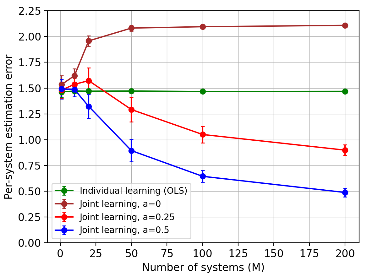
For generating the systems, we consider settings with the number of bases k=10k=10, dimension d=25d=25, trajectory length T=200T=200, and the number of systems M{1,10,20,50,100,200}M\in\{1,10,20,50,100,200\}. We simulate two cases:
(i) the spectral radii are in the range [0.7,0.9][0.7,0.9], and
(ii) all systems have an eigenvalue of magnitude 11.

The matrices {Wi}i=110\{W_{i}\}_{i=1}^{10} are generated randomly, such that each entry of WiW_{i} is sampled independently from the standard normal distribution N(0,1)N(0,1). Using these matrices, we generate MM systems by randomly generating the idiosyncratic components βm\beta_{m} from a standard normal distribution. For generating the state trajectories, noise vectors are isotropic Gaussian with variance 44. Additional numerical simulations using Bernoulli random matrices are provided in Appendix A.

We simulate the joint learning problem both with and without model misspecifications. For the latter, deviations from the shared structure are simulated by the components DmD_{m}, which are added randomly with probability 1/Ma1/M^{a} for a{0,0.25,0.5}a\in\{0,0.25,0.5\}. The matrices DmD_{m} are generated with independent Gaussian entries of variance 0.010.01, leading to DmF26.25{\left|\kern-1.29167pt\left|D_{m}\right|\kern-1.29167pt\right|}_{F}^{2}\approx 6.25 and ζ¯26.25M1a\bar{\zeta}^{2}\approx 6.25~{}M^{1-a}, according to the dimension d=25d=25.

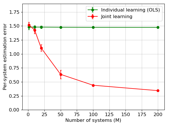
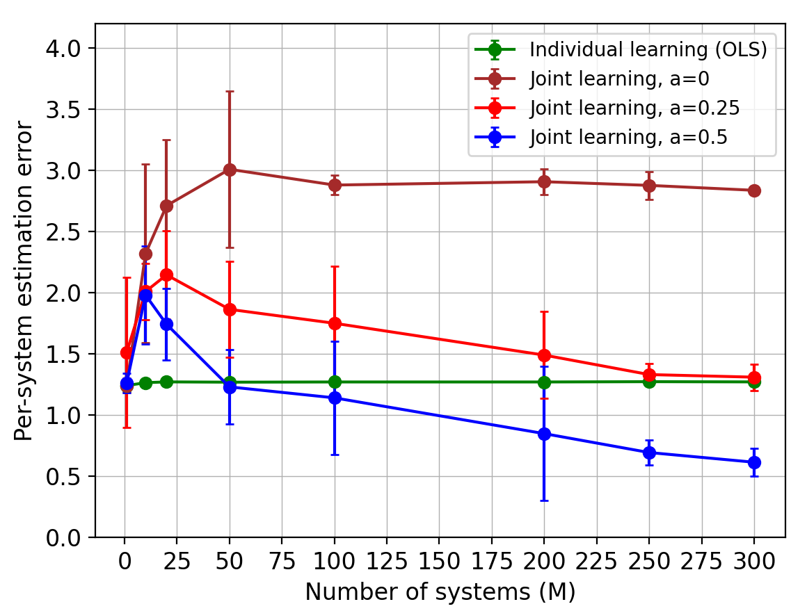
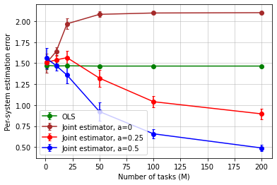
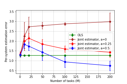
To report the results, for each value of MM in Figure 2 (resp. Figure 3), we average the errors from 1010 (resp. 2020) random replicates and plot the standard deviation as the error bar. Figure 2 depicts the estimation errors for both stable and unit-root transition matrices, versus MM. It can be seen that the joint estimator exhibits the expected improvement against the individual one.

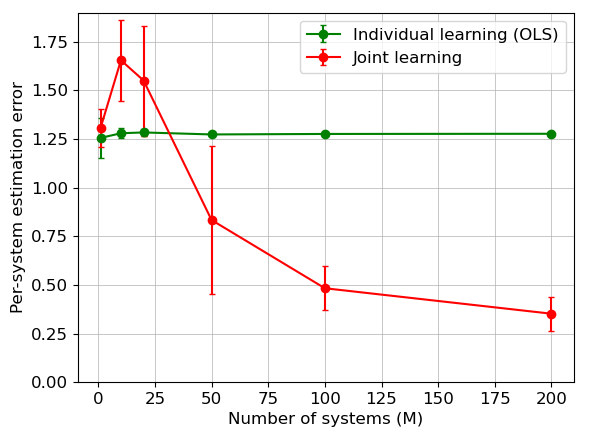
More interestingly, in Figure 3(a), we observe that for stable systems, the joint estimator performs worse than the individual one, when significant violations from the shared structure occurs in all systems (i.e., a=0a=0). Note that it corroborates Theorem 3, since in this case the total misspecification ζ¯2\bar{\zeta}^{2} scales linearly with MM. However, if the proportion of systems which violate the shared structure in Assumption 3 decreases, the joint estimation error improves as expected (a=0.25,0.5a=0.25,0.5).

Figure 3(b) depicts the estimation error for the joint estimator under misspecification for systems that have an eigenvalue on the unit circle in the complex plane. Our theoretical results suggest that the number of systems needs to be significantly larger in this case to circumvent the cost of misspecification in joint learning. The figure corroborates this result, wherein we observe that the joint estimation error is larger than the individual one, if all systems are misspecified (i.e., a=0a=0). Decreases in the total misspecification (i.e., a=0.25,0.5a=0.25,0.5) improves the error rate for joint learning, but requires larger number of systems than the stable case.

Refer to caption
Figure 4: Estimation and validation prediction errors versus the hyperparameter kk^{\prime}, for the true value k=10k=10.

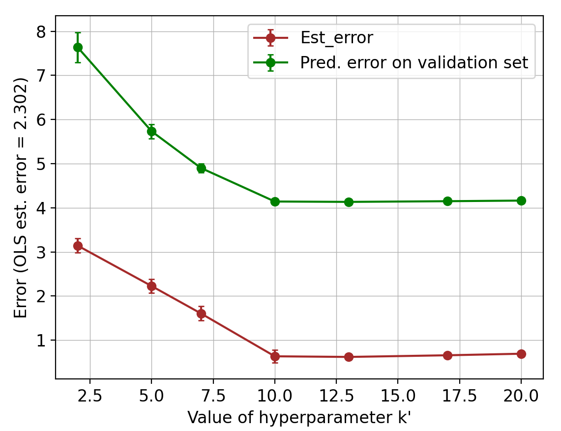
Finally, we discuss the choice of the number of bases kk for applying the joint estimator to real data. It can be handled by model selection methods such as elbow criterion and information criteria [2, 37], as well as robust estimation methods in panel data and factor models [12, 13]. In fact, for all kkk^{\prime}\geq k, the structural assumption is satisfied and leads to similar learning rates, while k<kk^{\prime}<k can lead to larger estimation errors. In Figure 4, we provide a simulation (with T=250,M=50T=250,M=50) and report the per-system estimation error, as well as the prediction error on a validation data (which is a subset of size 5050). Across all 1010 runs in the experiment, we observed that if the hyperparameter kk^{\prime} is chosen according to the elbow criteria, the resulting number of basis models is either equal to the true value k=10k=10, or slightly larger. For misspecified models, the optimal choice of kk^{\prime} can vary, in the sense that large misspecifications can be added to the shared basis (i.e., k>kk^{\prime}>k).

6 Proof of Theorem 1

In this and the following sections, we provide the detailed proofs for our results. We start by analysing the sample covariance matrix for each system which is then used to derive the estimation error rates in Theorem 2 and Theorem 3. For clarity, some details of the proofs are delegated to Appendix C. In Section 9, we provide the general probabilistic inequalities that are used throughout the proofs. Now, we prove high probability bounds for covariance matrices Σm=Σm(T)=t=0Txm(t)xm(t)\Sigma_{m}=\Sigma_{m}(T)=\sum_{t=0}^{T}x_{m}(t)x_{m}(t)^{\prime} in Theorem 1.

6.1 Upper Bounds on Covariance Matrices

To prove an upper bound on each system covariance matrix, we use an approach for LTI systems that relies on bounding norms of exponents of matrices [16]. Using lml_{m}^{*} and α(Am)\alpha(A_{m}) in (5) and ξm=|Pm1|2|Pm|\xi_{m}=\left|\!\left|\!\left|P_{m}^{-1}\right|\!\right|\!\right|_{{\infty\rightarrow 2}}\left|\!\left|\!\left|P_{m}\right|\!\right|\!\right|_{{\infty}}, the first step is to bound the sizes of all state vectors under the event bdd(δ)\mathcal{E}_{\mathrm{bdd}}(\delta) in Proposition 7.

Proposition 1 (Bounding xm(t){\left|\kern-1.29167pt\left|x_{m}(t)\right|\kern-1.29167pt\right|}).

For all t[T],m[M]t\in[T],m\in[M], under the event bdd(δ)\mathcal{E}_{\mathrm{bdd}}(\delta), we have:

xm(t){α(Am)b¯m(δ),if |λm,1|<1ρT,α(Am)b¯m(δ)tlm,if |λm,11|ρT.\displaystyle{\left|\kern-1.29167pt\left|x_{m}(t)\right|\kern-1.29167pt\right|}\leq\begin{cases}\alpha(A_{m})\bar{b}_{m}(\delta),&\text{if }~{}~{}|\lambda_{m,1}|<1-\frac{\rho}{T},\\ \alpha(A_{m})\bar{b}_{m}(\delta)t^{l^{*}_{m}},&\text{if }~{}~{}|\lambda_{m,1}-1|\leq\frac{\rho}{T}\end{cases}.

where b¯m(δ)=(bT(δ)+xm(0))\bar{b}_{m}(\delta)=\left(b_{T}(\delta)+{\left|\kern-1.29167pt\left|x_{m}(0)\right|\kern-1.29167pt\right|}_{\infty}\right).

Proof.

As before, each transition matrix AmA_{m} admits a Jordan normal form as follows: Am=Pm1ΛmPmA_{m}=P_{m}^{-1}\Lambda_{m}P_{m}, where Λm\Lambda_{m} is a block-diagonal matrix Λm=diag(Λm,q,,Λm,q)\Lambda_{m}={\rm diag}\left(\Lambda_{m,q},\ldots,\Lambda_{m,q}\right). Each Jordan block Λm,i\Lambda_{m,i} is of size lm,il_{m,i}. Note that for each system, the state vector satisfies:

xm(t)=\displaystyle x_{m}(t)={} s=1tAmtsηm(s)+Amtxm(0)\displaystyle\sum_{s=1}^{t}A_{m}^{t-s}\eta_{m}(s)+A_{m}^{t}x_{m}(0)
=\displaystyle={} s=1tPm1ΛmtsPmηm(s)+Pm1ΛmtPxm(0).\displaystyle\sum_{s=1}^{t}P_{m}^{-1}\Lambda_{m}^{t-s}P_{m}\eta_{m}(s)+P_{m}^{-1}\Lambda_{m}^{t}Px_{m}(0).

Now, letting bT(δ)b_{T}(\delta) be the same as in Proposition 7, we can bound the 2\ell_{2}-norm of the state vector as follows:

xm(t)\displaystyle{\left|\kern-1.29167pt\left|x_{m}(t)\right|\kern-1.29167pt\right|}\leq{} |Pm1|2|s=1tΛmts||Pm|bT(λ)\displaystyle\left|\!\left|\!\left|P_{m}^{-1}\right|\!\right|\!\right|_{{\infty\rightarrow 2}}\left|\!\left|\!\left|\sum_{s=1}^{t}\Lambda_{m}^{t-s}\right|\!\right|\!\right|_{{\infty}}\left|\!\left|\!\left|P_{m}\right|\!\right|\!\right|_{{\infty}}b_{T}(\lambda)
+|Pm1|2|Λmt||Pm|xm(0)\displaystyle+\left|\!\left|\!\left|P_{m}^{-1}\right|\!\right|\!\right|_{{\infty\rightarrow 2}}\left|\!\left|\!\left|\Lambda_{m}^{t}\right|\!\right|\!\right|_{{\infty}}\left|\!\left|\!\left|P_{m}\right|\!\right|\!\right|_{{\infty}}{\left|\kern-1.29167pt\left|x_{m}(0)\right|\kern-1.29167pt\right|}_{\infty}
\displaystyle\leq{} ξm(s=0t|Λmts|)(bT(δ)+xm(0)).\displaystyle\xi_{m}\left(\sum_{s=0}^{t}\left|\!\left|\!\left|\Lambda_{m}^{t-s}\right|\!\right|\!\right|_{{\infty}}\right)\big{(}b_{T}(\delta)+{\left|\kern-1.29167pt\left|x_{m}(0)\right|\kern-1.29167pt\right|}_{\infty}\big{)}.

For any matrix, the \ell_{\infty} norm is equal to the maximum row sum. Since the powers of a Jordan matrix will follow the same block structure as the original one, we can bound the operator norm |Amts|\left|\!\left|\!\left|A_{m}^{t-s}\right|\!\right|\!\right|_{{\infty}} by the norm of each block. The maximum row sum for the ss-th power of a Jordan block is: j=0l1(sj)λsj\sum_{j=0}^{l-1}\binom{s}{j}\lambda^{s-j}. Using this, we will bound the size of each state vector for the case when

  1. (I)

    the spectral radius of AmA_{m} satisfies |λ1(Am)|<1ρT\left|\lambda_{1}(A_{m})\right|<1-\frac{\rho}{T},

  2. (II)

    or, when |λ1(Am)1|ρT\left|\lambda_{1}(A_{m})-1\right|\leq\frac{\rho}{T}, for a constant ρ>0\rho>0.

Case I

When the Jordan block for a system matrix has eigenvalues strictly less than 1, we have:

s=0t|Λmts|\displaystyle\sum_{s=0}^{t}\left|\!\left|\!\left|\Lambda_{m}^{t-s}\right|\!\right|\!\right|_{{\infty}}\leq{} maxi[qm]s=0tj=0lm,i1(sj)|λm,i|sj\displaystyle\max_{i\in[q_{m}]}\sum_{s=0}^{t}\sum_{j=0}^{l_{m,i}-1}\binom{s}{j}\left|\lambda_{m,i}\right|^{s-j}
\displaystyle\leq{} s=0tj=0lm1(sj)|λm,1|sj\displaystyle\sum_{s=0}^{t}\sum_{j=0}^{l^{*}_{m}-1}\binom{s}{j}\left|\lambda_{m,1}\right|^{s-j}
\displaystyle\leq{} s=0t|λm,1|sj=0lm1sjj!|λm,1|j\displaystyle\sum_{s=0}^{t}\left|\lambda_{m,1}\right|^{s}\sum_{j=0}^{l^{*}_{m}-1}\frac{s^{j}}{j!}\left|\lambda_{m,1}\right|^{-j}
\displaystyle\leq{} s=0t|λm,1|sslm1j=0lm1|λm,1|jj!\displaystyle\sum_{s=0}^{t}\left|\lambda_{m,1}\right|^{s}s^{l^{*}_{m}-1}\sum_{j=0}^{l^{*}_{m}-1}\frac{\left|\lambda_{m,1}\right|^{-j}}{j!}
\displaystyle\leq{} e1/|λm,1|s=0|λm,1|sslm1\displaystyle e^{1/|\lambda_{m,1}|}\sum_{s=0}^{\infty}\left|\lambda_{m,1}\right|^{s}s^{l^{*}_{m}-1}
\displaystyle\lesssim{} e1/|λm,1|[lm1log|λm,1|+(lm1)!(log|λm,1|)lm].\displaystyle e^{1/|\lambda_{m,1}|}\left[\frac{l^{*}_{m}-1}{-\log|\lambda_{m,1}|}+\frac{(l^{*}_{m}-1)!}{(-\log|\lambda_{m,1}|)^{l^{*}_{m}}}\right].

Thus, for this case, each state vector can be upper bounded as xm(t)α(Am)(bT(δ)+xm(0)){\left|\kern-1.29167pt\left|x_{m}(t)\right|\kern-1.29167pt\right|}\leq\alpha(A_{m})(b_{T}(\delta)+{\left|\kern-1.29167pt\left|x_{m}(0)\right|\kern-1.29167pt\right|}_{\infty}). When the matrix AmA_{m} is diagonalizable, each Jordan block is of size 11, which leads to the upper-bound s=0t|Λmts|(1λ1)1\sum_{s=0}^{t}\left|\!\left|\!\left|\Lambda_{m}^{t-s}\right|\!\right|\!\right|_{{\infty}}\leq(1-\lambda_{1})^{-1}, for all t0t\geq 0. Therefore for diagonalizable AmA_{m}, we can let α(Am)=(1λ1)1|Pm1|2|Pm|\alpha(A_{m})=(1-\lambda_{1})^{-1}{\left|\!\left|\!\left|P_{m}^{-1}\right|\!\right|\!\right|_{{\infty\rightarrow 2}}\left|\!\left|\!\left|P_{m}\right|\!\right|\!\right|_{{\infty}}}.

Case II

When |λm,11|ρT\left|\lambda_{m,1}-1\right|\leq\frac{\rho}{T}, we get |λm,1|teρ\left|\lambda_{m,1}\right|^{t}\leq e^{\rho}, for all tTt\leq T. Therefore, since lml^{*}_{m} is the largest Jordan block, we have:

s=0t|Λmts|\displaystyle\sum_{s=0}^{t}\left|\!\left|\!\left|\Lambda_{m}^{t-s}\right|\!\right|\!\right|_{{\infty}}\leq{} s=0tj=0lm1(sj)|λm,1|sjeρs=0tj=0lm1(sj)\displaystyle\sum_{s=0}^{t}\sum_{j=0}^{l^{*}_{m}-1}\binom{s}{j}\left|\lambda_{m,1}\right|^{s-j}\leq{}e^{\rho}\sum_{s=0}^{t}\sum_{j=0}^{l^{*}_{m}-1}\binom{s}{j}
\displaystyle\leq{} eρs=0tj=0lm1sj/j!eρs=0tslm1j=0lm11/j!\displaystyle e^{\rho}\sum_{s=0}^{t}\sum_{j=0}^{l^{*}_{m}-1}s^{j}/j!\leq{}e^{\rho}\sum_{s=0}^{t}s^{l^{*}_{m}-1}\sum_{j=0}^{l^{*}_{m}-1}1/j!
\displaystyle\leq{} eρ+1s=0tslm1eρ+1tlm.\displaystyle e^{\rho+1}\sum_{s=0}^{t}s^{l^{*}_{m}-1}\lesssim{}e^{\rho+1}t^{l^{*}_{m}}.

Therefore, the magnitude of each state vector grows polynomially with tt, the exponent being at most lml^{*}_{m}. For example, when AmA_{m} is diagonalizable, the Jordan block for the unit root is of size 11, givin s=0t|Λmts|eρt\sum_{s=0}^{t}\left|\!\left|\!\left|\Lambda_{m}^{t-s}\right|\!\right|\!\right|_{{\infty}}\leq e^{\rho}t.

So, for systems with unit roots, the bound on each state vector is as expressed in the proposition. ∎

Using the high probability upper bound on the size of each state vector, we can upper bound the covariance matrix for each system as follows:

Lemma 1 (Upper bound on Σm\Sigma_{m}).

For all m[M]m\in[M], the sample covariance matrix Σm\Sigma_{m} of system mm can be upper bounded under the event bdd(δ)\mathcal{E}_{\mathrm{bdd}}(\delta), as follows:

  1. (I)

    When all eigenvalues of the matrix AmA_{m} are strictly less than 11 in magnitude (|λm,i|<1ρT|\lambda_{m,i}|<1-\frac{\rho}{T}), we have

    λmax(Σm)α(Am)2(bT(δ)+xm(0))2T.\displaystyle\lambda_{\max}(\Sigma_{m})\leq\alpha(A_{m})^{2}\left(b_{T}(\delta)+{\left|\kern-1.29167pt\left|x_{m}(0)\right|\kern-1.29167pt\right|}_{\infty}\right)^{2}T.
  2. (II)

    When some eigenvalues of the matrix AmA_{m} are close to 11, i.e. |λ1(Am)1|ρT|\lambda_{1}(A_{m})-1|\leq\frac{\rho}{T}, we have:

    λmax(Σm)α(Am)2(bT(δ)+xm(0))2T2lm,1+1.\displaystyle\lambda_{\max}(\Sigma_{m})\leq\alpha(A_{m})^{2}\left(b_{T}(\delta)+{\left|\kern-1.29167pt\left|x_{m}(0)\right|\kern-1.29167pt\right|}_{\infty}\right)^{2}T^{2l_{m,1}+1}.
Proof.

First note that we have:

λmax(Σm)=|t=0Txm(t)xm(t)|2t=0Txm(t)22.\displaystyle\lambda_{\max}(\Sigma_{m})=\left|\!\left|\!\left|\sum_{t=0}^{T}x_{m}(t)x_{m}(t)^{\prime}\right|\!\right|\!\right|_{{2}}\leq\sum_{t=0}^{T}{\left|\kern-1.29167pt\left|x_{m}(t)\right|\kern-1.29167pt\right|}_{2}^{2}.

Therefore, by Proposition 7, when all eigenvalues of AmA_{m} are strictly less than 11, we have:

λmax(Σm)Tα(Am)2(bT(δ)+xm(0))2.\displaystyle\lambda_{\max}(\Sigma_{m})\leq T\alpha(A_{m})^{2}\left(b_{T}(\delta)+{\left|\kern-1.29167pt\left|x_{m}(0)\right|\kern-1.29167pt\right|}_{\infty}\right)^{2}.

For the case when 1ρTλ1(Am)1+ρT1-\frac{\rho}{T}\leq\lambda_{1}(A_{m})\leq 1+\frac{\rho}{T}, we get:

λmax(Σm)\displaystyle\lambda_{\max}(\Sigma_{m})\leq{} α(Λm)2t=0Tt2lm,1\displaystyle\alpha(\Lambda_{m})^{2}\sum_{t=0}^{T}t^{2l_{m,1}}
\displaystyle\leq{} α(Am)2(bT(δ)+xm(0))2T2lm,1+1.\displaystyle\alpha(A_{m})^{2}\left(b_{T}(\delta)+{\left|\kern-1.29167pt\left|x_{m}(0)\right|\kern-1.29167pt\right|}_{\infty}\right)^{2}T^{2l_{m,1}+1}.

6.2 Lower Bound for Covariance Matrices

A lower bound result for the idiosyncratic covariance matrices can be derived using the probabilistic inequalities in the last section. We provide a detailed proof below.

Lemma 2 (Covariance lower bound.).

Define ϰ=dσ2λmin(C)2\varkappa=\tfrac{d\sigma^{2}}{\lambda_{\min}(C)^{2}}. For all m[M]m\in[M], if the per-system sample size TT is greater than T0T_{0} defined as

ϰmax(cηlog18δ,16(log(α(A)2b¯m(δ)2+1)+2log5δ)),\displaystyle\varkappa\cdot{\max}\left(c_{\eta}\log\tfrac{18}{\delta},16\left(\log\left(\alpha(A)^{2}\bar{b}_{m}(\delta)^{2}+1\right)+2\log\tfrac{5}{\delta}\right)\right),

if |λm,1|<1ρT\left|\lambda_{m,1}\right|<1-\frac{\rho}{T}, and

ϰmax(cηlog18δ,16(log(α(A)2b¯m(δ)2T2lm+1)+2log5δ))\displaystyle\varkappa\cdot{\max}\left(c_{\eta}\log\tfrac{18}{\delta},16\left(\log\left(\alpha(A)^{2}\bar{b}_{m}(\delta)^{2}T^{2l^{*}_{m}}+1\right)+2\log\tfrac{5}{\delta}\right)\right)

if 1ρT|λm,1|1+ρT1-\frac{\rho}{T}\leq\left|\lambda_{m,1}\right|\leq 1+\frac{\rho}{T}, then with probability at least 13δ1-3\delta, the sample covariance matrix Σm\Sigma_{m} for system mm can be bounded from below: Σm(T)Tλmin(C)4I\Sigma_{m}(T)\succeq\frac{T\lambda_{\min}(C)}{4}I.

Proof.

We bound the covariance matrix under the events bdd(δ)\mathcal{E}_{\mathrm{bdd}}(\delta), η(δ)\mathcal{E}_{\eta}(\delta) in Propositions 7, 8, as well as the one in Proposition 10. As we consider a bound for all systems, we drop the system subscript mm here. Using (1), we have:

Σ(T)\displaystyle\Sigma(T)\succeq{} AΣ(T1)A+t=1Tη(t)η(t)\displaystyle A\Sigma(T-1)A^{\prime}+\sum_{t=1}^{T}\eta(t)\eta(t)^{\prime}
+t=0T1(Ax(t)η(t+1)+η(t+1)x(t)A)\displaystyle+\sum_{t=0}^{T-1}\left(Ax(t)\eta(t+1)^{\prime}+\eta(t+1)x(t)^{\prime}A^{\prime}\right)

Since Tϰcηlog18δ=cηdσ2log18δλmin(C)2T\geq\varkappa c_{\eta}\log\frac{18}{\delta}=\frac{c_{\eta}d\sigma^{2}\log\frac{18}{\delta}}{\lambda_{\min}(C)^{2}}, under the event η(δ)\mathcal{E}_{\eta}(\delta) it holds that

Σ(T)\displaystyle\Sigma(T)\succeq{} AΣ(T1)A+3λmin(C)T4\displaystyle A\Sigma(T-1)A^{\prime}+\frac{3\lambda_{\min}(C)T}{4}
+t=0T1(Ax(t)η(t+1)+η(t+1)x(t)A).\displaystyle+\sum_{t=0}^{T-1}\left(Ax(t)\eta(t+1)^{\prime}+\eta(t+1)x(t)^{\prime}A^{\prime}\right).

Thus, for any unit vector uu (i.e., on the unit sphere 𝒮d1{\mathcal{S}}^{d-1}), we have

uΣ(T)u\displaystyle u^{\prime}\Sigma(T)u\geq{} uAΣ(T1)Au+3λmin(C)T4\displaystyle u^{\prime}A\Sigma(T-1)A^{\prime}u+\frac{3\lambda_{\min}(C)T}{4}
+t=0T1u(Ax(t)η(t+1)+η(t+1)x(t)A)u.\displaystyle+\sum_{t=0}^{T-1}u^{\prime}\left(Ax(t)\eta(t+1)^{\prime}+\eta(t+1)x(t)^{\prime}A^{\prime}\right)u.

Now, by Proposition 10 with V=TIV=T\cdot I, we get the following result for the martingale t=0T1AmXm(t)ηm(t+1)\sum_{t=0}^{T-1}A_{m}X_{m}(t)\eta_{m}(t+1)^{\prime} and V¯m(s)t=0sAmXm(t)Xm(t)Am+V\bar{V}_{m}(s)\coloneqq\sum_{t=0}^{s}A_{m}X_{m}(t)X_{m}(t)^{\prime}A_{m}^{\prime}+V, with probability at least 1δ1-\delta:

t=0T1Ax(t)η(t+1)u\displaystyle{\left|\kern-1.29167pt\left|\sum_{t=0}^{T-1}Ax(t)\eta(t+1)^{\prime}u\right|\kern-1.29167pt\right|}
\displaystyle\leq{} uAΣ(T1)Au+T\displaystyle\sqrt{u^{\prime}A\Sigma(T-1)A^{\prime}u+T}
8dσ2log(5det(V¯m(T1))1/2ddet(TI)1/2dδ1/d).\displaystyle\sqrt{8d\sigma^{2}\log\left(\frac{5\det\left(\bar{V}_{m}(T-1)\right)^{1/2d}\det\left(TI\right)^{-1/2d}}{\delta^{1/d}}\right)}.

Thus, we get:

uΣ(T)u\displaystyle u^{\prime}\Sigma(T)u
\displaystyle\succeq{} uAΣ(T1)AuuAΣ(T1)Au+T\displaystyle u^{\prime}A\Sigma(T-1)A^{\prime}u-\sqrt{u^{\prime}A\Sigma(T-1)A^{\prime}u+T}
16dσ2log(λmax(V¯(T1))T)+32dσ2log5δ+3λmin(C)T4.\displaystyle\sqrt{16d\sigma^{2}\log\left(\tfrac{\lambda_{\max}(\bar{V}(T-1))}{T}\right)+32d\sigma^{2}\log\tfrac{5}{\delta}}+\frac{3\lambda_{\min}(C)T}{4}.

Hence, we have:

uΣ(T)Tu\displaystyle u^{\prime}\frac{\Sigma(T)}{T}u\succeq{} uAΣ(T1)ATu+3λmin(C)4\displaystyle u^{\prime}\frac{A\Sigma(T-1)A^{\prime}}{T}u+\frac{3\lambda_{\min}(C)}{4}
uAΣ(T1)ATu+1λmin(C)2\displaystyle-\sqrt{u^{\prime}\frac{A\Sigma(T-1)A^{\prime}}{T}u+1}\frac{\lambda_{\min}(C)}{2}
\displaystyle\succeq{} λmin(C)4,\displaystyle\frac{\lambda_{\min}(C)}{4},

whenever TT is larger than

16dσ2λmin(C)2(log(λmax(V¯(T1))T)+2log5δ)\displaystyle\frac{16d\sigma^{2}}{\lambda_{\min}(C)^{2}}\left(\log\left(\frac{\lambda_{\max}(\bar{V}(T-1))}{T}\right)+2\log\frac{5}{\delta}\right)
=\displaystyle={} 16dσ2λmin(C)2(log(λmax(t=0T1AX(t)X(t)A)T+1)+2log5δ).\displaystyle\tfrac{16d\sigma^{2}}{\lambda_{\min}(C)^{2}}\left(\log\left(\tfrac{\lambda_{\max}\left(\sum_{t=0}^{T-1}AX(t)X(t)^{\prime}A^{\prime}\right)}{T}+1\right)+2\log\tfrac{5}{\delta}\right).

Using the upper bound analysis in Lemma 1, we show that it suffices for TT to be lower bounded as

T16dσ2λmin(C)2(log(α(A)2b¯m(δ)2+1)+2log5δ),\displaystyle T\geq\frac{16d\sigma^{2}}{\lambda_{\min}(C)^{2}}\left(\log\left(\alpha(A)^{2}\bar{b}_{m}(\delta)^{2}+1\right)+2\log\frac{5}{\delta}\right),

when AA is strictly stable, and as

T16dσ2λmin(C)2(log(α(A)2b¯m(δ)2T2l+1)+2log5δ),\displaystyle T\geq\frac{16d\sigma^{2}}{\lambda_{\min}(C)^{2}}\left(\log\left(\alpha(A)^{2}\bar{b}_{m}(\delta)^{2}T^{2l^{*}}+1\right)+2\log\frac{5}{\delta}\right),

when |λ1(A)|1+ρT\left|\lambda_{1}(A)\right|\leq 1+\frac{\rho}{T}. Since, both quantities on the RHS grow at most logarithmically with TT, there exists T0T_{0} such that it holds for all TT0T\geq T_{0}. Combining the failure probability for all events, we get the desired result. ∎

7 Proof of Theorem 2

In this section, we use the result in Theorem 1 to analyze the estimation error for the estimator in (3), under Assumption 3. For ease of presentation, we rewrite the problem by transforming the vector output space to scalar values. For that purpose, we introduce some notation to express transition matrices in vector form and rewrite (3). First, for each state vector xm(t)dx_{m}(t)\in\mathbb{R}^{d}, we create dd different covariates of size d2\mathbb{R}^{d^{2}}. So, for j=1,,dj=1,\cdots,d, the vector x~m,j(t)d2\tilde{x}_{m,j}(t)\in\mathbb{R}^{d^{2}} contains xm(t)x_{m}(t) in the jj-th block of size dd and 0s0^{\prime}s elsewhere.

Then, we express the system matrix Amd×dA_{m}\in\mathbb{R}^{d\times d} as a vector A~md2\tilde{A}_{m}\in\mathbb{R}^{d^{2}}. Similarly, the concatenation of all vectors A~m\tilde{A}_{m} can be coalesced into the matrix Θ~d2×M\tilde{\Theta}\in\mathbb{R}^{d^{2}\times M}. Analogously, η~m(t)\tilde{\eta}_{m}(t) will denote the concatenated dtdt dimensional vector of noise vectors for system mm. Thus, the structural assumption in (2) can be written as:

A~m=Wβm,\displaystyle\tilde{A}_{m}=W^{*}\beta^{*}_{m}, (12)

where Wd2×kW^{*}\in\mathbb{R}^{d^{2}\times k} and βmk\beta^{*}_{m}\in\mathbb{R}^{k}. Similarly, the overall parameter set can be factorized as Θ~=WB\tilde{\Theta}^{*}=W^{*}B^{*}, where the matrix B=[β1|β2|βM]k×MB^{*}=[\beta^{*}_{1}|\beta^{*}_{2}|\cdots\beta^{*}_{M}]\in\mathbb{R}^{k\times M} contains the true weight vectors βm\beta^{*}_{m}. Thus, expressing the system matrices AmA_{m} in this manner leads to a low rank structure in (12), so that the matrix Θ~\tilde{\Theta}^{*} is of rank kk. Using the vectorized parameters, the evolution for the components j[d]j\in[d] of all state vectors xm(t)x_{m}(t) can be written as:

xm(t+1)[j]=A~mx~m,j(t)+ηm(t+1)[j].\displaystyle x_{m}(t+1)[j]=\tilde{A}_{m}\tilde{x}_{m,j}(t)+\eta_{m}(t+1)[j]. (13)

For each system m[M]m\in[M], we therefore have a total of dTdT samples, where the statistical dependence now follows a block structure: dd covariates of xm(1)x_{m}(1) are all constructed using xm(0)x_{m}(0), next dd using xm(1)x_{m}(1) and so forth. To estimate the parameters, we solve the following optimization problem:

W^,{β^m}m=1M\displaystyle\widehat{W},\{\widehat{\beta}_{m}\}_{m=1}^{M}
\displaystyle\coloneqq argminW,{βm}m=1Mm,tj=1d(xm(t+1)[j]Wβm,x~m,j(t))2(W,β)\displaystyle{}\mathop{\mathrm{argmin}}_{W,\{\beta_{m}\}_{m=1}^{M}}\underbrace{\sum_{m,t}\sum_{j=1}^{d}\left(x_{m}(t+1)[j]-\langle W\beta_{m},\tilde{x}_{m,j}(t)\rangle\right)^{2}}_{\mathcal{L}(W,\beta)}
=\displaystyle= argminW,{βm}m=1Mm=1MymX~mWβm22,\displaystyle{}\mathop{\mathrm{argmin}}_{W,\{\beta_{m}\}_{m=1}^{M}}\sum_{m=1}^{M}\left\|y_{m}-\tilde{X}_{m}W\beta_{m}\right\|_{2}^{2}, (14)

where ymTdy_{m}\in\mathbb{R}^{Td} contains all TT state vectors stacked vertically and X~mTd×d2\tilde{X}_{m}\in\mathbb{R}^{Td\times d^{2}} contains the corresponding matrix input. We denote the covariance matrices for the vectorized form by Σ~m=t=0T1x~m(t)x~m(t)\tilde{\Sigma}_{m}=\sum_{t=0}^{T-1}\tilde{x}_{m}(t)\tilde{x}_{m}(t)^{\prime}. Recall, that the sample covariance matrices for all systems are denoted by Σm=t=0T1xm(t)xm(t)\Sigma_{m}=\sum_{t=0}^{T-1}x_{m}(t)x_{m}(t)^{\prime}

We further use the following notation: for any parameter set Θ=WBd2×M\Theta=WB\in\mathbb{R}^{d^{2}\times M}, we define 𝒳(Θ)dT×M\mathcal{X}(\Theta)\in\mathbb{R}^{dT\times M} as 𝒳(Θ)[𝒳1(Θ)|𝒳2(Θ)|𝒳M(Θ)]\mathcal{X}(\Theta)\coloneqq\left[\mathcal{X}_{1}(\Theta)|\mathcal{X}_{2}(\Theta)\cdots|\mathcal{X}_{M}(\Theta)\right], where each column 𝒳m(Θ)dT\mathcal{X}_{m}(\Theta)\in\mathbb{R}^{dT} is the prediction of states xm(t+1)x_{m}(t+1) with Θm\Theta_{m}. That is,

𝒳m(Θ)=(xm(0),xm(0)Θm,,xm(T1)Θm).\mathcal{X}_{m}(\Theta)=(x_{m}(0)^{\prime},x_{m}(0)^{\prime}\Theta_{m}^{\prime},\ldots,x_{m}(T-1)^{\prime}\Theta_{m}^{\prime})^{\prime}.

Thus, 𝒳(Θ~)Td×M\mathcal{X}(\tilde{\Theta}^{*})\in\mathbb{R}^{Td\times M} denotes the ground truth mapping for the training data of the MM systems and 𝒳(Θ~Θ^)Td×M\mathcal{X}(\tilde{\Theta}^{*}-\widehat{\Theta})\in\mathbb{R}^{Td\times M} is the prediction error across all coordinates of the MTMT state vectors that each of which is of dimension dd.

By Assumption 3, we have ΔΘ~Θ^=UR\Delta\coloneqq\tilde{\Theta}^{*}-\widehat{\Theta}=UR, where UOd2×2kU\in O^{d^{2}\times 2k} is an orthonormal matrix and R2k×MR\in\mathbb{R}^{2k\times M}. We start by the fact that the estimates W^\widehat{W} and β^m\widehat{\beta}_{m} minimize (3), and therefore, have a smaller squared prediction error than (W,B)(W^{*},B^{*}). Hence, we get the following inequality:

12m=1MX~m(WβmW^β^m)22\displaystyle\frac{1}{2}\sum_{m=1}^{M}{\left|\kern-1.29167pt\left|\tilde{X}_{m}(W^{*}\beta^{*}_{m}-\widehat{W}\widehat{\beta}_{m})\right|\kern-1.29167pt\right|}_{2}^{2}
\displaystyle\leq m=1Mη~m,X~m(W^β^mWβm).\displaystyle{}\sum_{m=1}^{M}\left\langle\tilde{\eta}_{m},\tilde{X}_{m}\left(\widehat{W}\widehat{\beta}_{m}-W^{*}\beta^{*}_{m}\right)\right\rangle. (15)

We can rewrite W^β^mWβm=Urm\widehat{W}\widehat{\beta}_{m}-W^{*}\beta^{*}_{m}=Ur_{m}, for all m[M]m\in[M], where rm2kr_{m}\in\mathbb{R}^{2k} is an idiosyncratic projection vector for system mm. Since our joint estimator is a least squares objective with bilinear terms, we first decompose the prediction error for the estimator, similar to the linear regression setting [14, 44]. In subsequent analyses, we use different matrix concentration results and LTI estimation theory in order to account for the temporal dependence and spectral properties of the systems. Our first step is to bound the prediction error for all systems.

Lemma 3.

For any fixed orthonormal matrix U¯d2×2k\bar{U}\in\mathbb{R}^{d^{2}\times 2k}, the total squared prediction error in (3) for (W^,B^)(\widehat{W},\widehat{B}) can be decomposed as follows:

12m=1MX~m(WβmW^β^m)F2\displaystyle\frac{1}{2}\sum_{m=1}^{M}{\left|\kern-1.29167pt\left|\tilde{X}_{m}(W^{*}\beta^{*}_{m}-\widehat{W}\widehat{\beta}_{m})\right|\kern-1.29167pt\right|}_{F}^{2}
\displaystyle\leq{} m=1Mη~mX~mU¯V¯m122m=1MX~m(WβmW^β^m)22\displaystyle\sqrt{\sum_{m=1}^{M}{\left|\kern-1.29167pt\left|\tilde{\eta}_{m}^{\top}\tilde{X}_{m}\bar{U}\right|\kern-1.29167pt\right|}_{\bar{V}^{-1}_{m}}^{2}}\sqrt{2\sum_{m=1}^{M}{\left|\kern-1.29167pt\left|\tilde{X}_{m}(W^{*}\beta^{*}_{m}-\widehat{W}\widehat{\beta}_{m})\right|\kern-1.29167pt\right|}_{2}^{2}}
+m=1Mη~mX~mU¯V¯m12m=1MX~m(U¯U)rm2\displaystyle+\sqrt{\sum_{m=1}^{M}{\left|\kern-1.29167pt\left|\tilde{\eta}_{m}^{\top}\tilde{X}_{m}\bar{U}\right|\kern-1.29167pt\right|}_{\bar{V}^{-1}_{m}}^{2}}\sqrt{\sum_{m=1}^{M}{\left|\kern-1.29167pt\left|\tilde{X}_{m}(\bar{U}-U)r_{m}\right|\kern-1.29167pt\right|}^{2}}
+m=1Mη~m,X~m(UU¯)rm.\displaystyle+\sum_{m=1}^{M}\left\langle\tilde{\eta}_{m},\tilde{X}_{m}(U-\bar{U})r_{m}\right\rangle. (16)

The proof of Lemma 3 can be found in the extended version of this paper [34]. Our next step is to bound each term on the RHS of (16). To that end, let 𝒩ϵ\mathcal{N}_{\epsilon} be an ϵ\epsilon-cover of the set of orthonormal matrices in d2×2k\mathbb{R}^{d^{2}\times 2k}. In (16), we select the matrix U¯\bar{U} to be an element of 𝒩ϵ\mathcal{N}_{\epsilon} such that U¯UFϵ{\left|\kern-1.29167pt\left|\bar{U}-U\right|\kern-1.29167pt\right|}_{F}\leq\epsilon. Note that since 𝒩ϵ\mathcal{N}_{\epsilon} is an ϵ\epsilon-cover, such matrix U¯\bar{U} exists. We can bound the size of such a cover using Lemma 5, and obtain |𝒩ϵ|(6dϵ)2d2k|\mathcal{N}_{\epsilon}|\leq\left(\frac{6\sqrt{d}}{\epsilon}\right)^{2d^{2}k}.

We now bound each term in the following propositions using the auxiliary results in Section 9 and covariance matrix bounds in the previous section. The detailed proofs for all of the following results are available in the extended version [34]. Using Proposition 9, we bound the following expression in the second term of (16), as follows.

Proposition 2.

Under Assumption 3, for the noise process {ηm(t)}t=1\{\eta_{m}(t)\}_{t=1}^{\infty} defined for each system, with probability at least 1δZ1-\delta_{Z}, we have:

m=1MX~m(U¯U)rm2\displaystyle\sum_{m=1}^{M}{\left|\kern-1.29167pt\left|\tilde{X}_{m}(\bar{U}-U)r_{m}\right|\kern-1.29167pt\right|}^{2}\lesssim{} 𝜿ϵ2(MTtr(C)+σ2log2δZ).\displaystyle\bm{\kappa}\epsilon^{2}\left(MT\mathop{\mathrm{tr}}\left(C\right)+\sigma^{2}\log\frac{2}{\delta_{Z}}\right).

Based on the bound in Proposition 2, we can bound the third term in (16) as follows:

Proposition 3.

Under Assumption 2 and Assumption 3, with probability at least 1δZ1-\delta_{Z}, we have:

m=1Mη~m,X~m(UU¯)rm\displaystyle\sum_{m=1}^{M}\left\langle\tilde{\eta}_{m},\tilde{X}_{m}(U-\bar{U})r_{m}\right\rangle\lesssim{} 𝜿ϵ(MTtr(C)+σ2log1δZ).\displaystyle\sqrt{\bm{\kappa}}\epsilon\left(MT\mathop{\mathrm{tr}}\left(C\right)+\sigma^{2}\log\tfrac{1}{\delta_{Z}}\right). (17)

Next, we show a multitask concentration of martingales projected on a low-rank subspace.

Proposition 4.

For an arbitrary orthonormal matrix U¯d2×2k\bar{U}\in\mathbb{R}^{d^{2}\times 2k} in the ϵ\epsilon-cover 𝒩ϵ\mathcal{N}_{\epsilon} defined in Lemma 5, let Σd2×d2\Sigma\in\mathbb{R}^{d^{2}\times d^{2}} be a positive definite matrix, and define Sm(τ)=η~m(τ)X~m(τ)U¯S_{m}(\tau)=\tilde{\eta}_{m}(\tau)^{\top}\tilde{X}_{m}(\tau)\bar{U}, V¯m(τ)=U¯(Σ~m(τ)+Σ)U¯\bar{V}_{m}(\tau)=\bar{U}^{\prime}\left(\tilde{\Sigma}_{m}(\tau)+\Sigma\right)\bar{U}, and V0=U¯ΣU¯V_{0}=\bar{U}^{\prime}\Sigma\bar{U}. Then, letting 1(δU)\mathcal{E}_{1}(\delta_{U}) be the event

m=1MSm(T)V¯m1(T)22σ2log(Πm=1Mdet(V¯m(T))det(V0)δU),\displaystyle\sum_{m=1}^{M}{\left|\kern-1.29167pt\left|S_{m}(T)\right|\kern-1.29167pt\right|}_{\bar{V}_{m}^{-1}(T)}^{2}\leq 2\sigma^{2}\log\left(\frac{\Pi_{m=1}^{M}\frac{\det(\bar{V}_{m}(T))}{\det(V_{0})}}{\delta_{U}}\right),

we have

[1(δU)]1(62kϵ)2d2kδU.\displaystyle\mathbb{P}\left[\mathcal{E}_{1}(\delta_{U})\right]\geq 1-\left(\frac{6\sqrt{2k}}{\epsilon}\right)^{2d^{2}k}\delta_{U}. (18)

7.1 Proof of Estimation Error in Theorem 2

Proof.

We now use the bounds we have shown for each term before and give the final steps by using the error decomposition in Lemma 3. Let |𝒩ϵ|\left|\mathcal{N}_{\epsilon}\right| be the cardinality of the ϵ\epsilon-cover of the set of orthonormal matrices in d2×2k\mathbb{R}^{d^{2}\times 2k} that we defined in Lemma 3. Let 𝕍\mathbb{V} denote the expression Πm=1Mdet(V¯m(t))det(V0)\Pi_{m=1}^{M}\frac{\det(\bar{V}_{m}(t))}{\det(V_{0})}. So, substituting the termwise bounds from Proposition 2, Proposition 3, and Proposition 4 in Lemma 3, with probability at least 1|𝒩ϵ|δUδZ1-\left|\mathcal{N}_{\epsilon}\right|\delta_{U}-\delta_{Z}, it holds that:

12𝒳(WBW^B^)F2\displaystyle\frac{1}{2}{\left|\kern-1.29167pt\left|\mathcal{X}(W^{*}B^{*}-\widehat{W}\widehat{B})\right|\kern-1.29167pt\right|}_{F}^{2}
\displaystyle\lesssim{} σ2log(𝕍δU)𝒳(WBW^B^)F\displaystyle\sqrt{\sigma^{2}\log\left(\frac{\mathbb{V}}{\delta_{U}}\right)}{\left|\kern-1.29167pt\left|\mathcal{X}(W^{*}B^{*}-\widehat{W}\widehat{B})\right|\kern-1.29167pt\right|}_{F}
+σ2log(𝕍δU)𝜿ϵ2(MTtr(C)+σ2log1δZ)\displaystyle+\sqrt{\sigma^{2}\log\left(\frac{\mathbb{V}}{\delta_{U}}\right)}\sqrt{\bm{\kappa}\epsilon^{2}\left(MT\mathop{\mathrm{tr}}\left(C\right)+\sigma^{2}\log\frac{1}{\delta_{Z}}\right)}
+𝜿ϵ(MTtr(C)+σ2log1δZ).\displaystyle+\sqrt{\bm{\kappa}}\epsilon\left(MT\mathop{\mathrm{tr}}\left(C\right)+\sigma^{2}\log\frac{1}{\delta_{Z}}\right). (19)

For the matrix V0V_{0}, we now substitute Σ=λ¯Id2\Sigma=\mkern 1.5mu\underline{\mkern-1.5mu\lambda\mkern-1.5mu}\mkern 1.5muI_{d^{2}}, which implies that det(V0)1=det(1/λ¯I2k)=(1/λ¯)2k\det(V_{0})^{-1}=\det(1/\mkern 1.5mu\underline{\mkern-1.5mu\lambda\mkern-1.5mu}\mkern 1.5muI_{2k})=\left(1/\mkern 1.5mu\underline{\mkern-1.5mu\lambda\mkern-1.5mu}\mkern 1.5mu\right)^{2k}. Similarly, for the matrix V¯m(T)\bar{V}_{m}(T), we get det(V¯m(T))λ¯2k\det(\bar{V}_{m}(T))\leq\bar{\lambda}^{2k}. Thus, substituting δU=31δ|𝒩|ϵ1\delta_{U}=3^{-1}\delta\left|\mathcal{N}\right|_{\epsilon}^{-1} and δC=31δ\delta_{C}=3^{-1}\delta in Theorem 1, with probability at least 12δ/31-2\delta/3, the upper-bound in Proposition 4 becomes:

m=1Mη~mX~mU¯V¯m12\displaystyle\sum_{m=1}^{M}{\left|\kern-1.29167pt\left|\tilde{\eta}_{m}^{\top}\tilde{X}_{m}\bar{U}\right|\kern-1.29167pt\right|}_{\bar{V}^{-1}_{m}}^{2}\leq{} σ2log(Πm=1Mdet(V¯m(t))det(V0)δU)\displaystyle\sigma^{2}\log\left(\frac{\Pi_{m=1}^{M}\frac{\det(\bar{V}_{m}(t))}{\det(V_{0})}}{\delta_{U}}\right)
\displaystyle\lesssim{} σ2Mklog𝜿+σ2d2klogkδϵ.\displaystyle\sigma^{2}Mk\log\bm{\kappa}_{\infty}+\sigma^{2}d^{2}k\log\frac{k}{\delta\epsilon}.

Substituting this in (19) with δZ=δ/3\delta_{Z}=\delta/3, c2=max(σ2,λ1(C))c^{2}=\max(\sigma^{2},\lambda_{1}(C)), with probability at least 1δ1-\delta, we have:

12𝒳(WBW^B^)F2\displaystyle\frac{1}{2}{\left|\kern-1.29167pt\left|\mathcal{X}(W^{*}B^{*}-\widehat{W}\widehat{B})\right|\kern-1.29167pt\right|}_{F}^{2}
\displaystyle\lesssim{} c2Mklog𝜿+c2d2klogkδϵ(||𝒳(WBW^B^)||F\displaystyle\sqrt{c^{2}Mk\log\bm{\kappa}_{\infty}+c^{2}d^{2}k\log\frac{k}{\delta\epsilon}}\Bigg{(}{\left|\kern-1.29167pt\left|\mathcal{X}(W^{*}B^{*}-\widehat{W}\widehat{B})\right|\kern-1.29167pt\right|}_{F}
+𝜿ϵ2(c2dMT+c2log1δ))\displaystyle+\sqrt{\bm{\kappa}\epsilon^{2}\left(c^{2}dMT+c^{2}\log\frac{1}{\delta}\right)}\Bigg{)}
+𝜿ϵ(c2dMT+c2log1δ).\displaystyle+\sqrt{\bm{\kappa}}\epsilon\left(c^{2}dMT+c^{2}\log\frac{1}{\delta}\right).

Noting that log1δd2klogkδϵ\log\frac{1}{\delta}\lesssim d^{2}k\log\frac{k}{\delta\epsilon} for ϵ=k𝜿d2T\epsilon=\frac{k}{\sqrt{\bm{\kappa}}d^{2}T}, with probability at least 1δ1-\delta, we get:

12𝒳(WBW^B^)F2\displaystyle\frac{1}{2}{\left|\kern-1.1625pt\left|\mathcal{X}(W^{*}B^{*}-\widehat{W}\widehat{B})\right|\kern-1.1625pt\right|}_{F}^{2}
\displaystyle\lesssim{} (c2Mklog𝜿+c2d2klog𝜿dTδ)𝒳(WBW^B^)F\displaystyle\left(\sqrt{c^{2}Mk\log\bm{\kappa}_{\infty}+c^{2}d^{2}k\log\tfrac{\bm{\kappa}dT}{\delta}}\right){\left|\kern-1.1625pt\left|\mathcal{X}(W^{*}B^{*}-\widehat{W}\widehat{B})\right|\kern-1.1625pt\right|}_{F}
+c2Mklog𝜿+c2d2klog𝜿dTδc2(k2Md3T+k3d2T2log𝜿dTδ)\displaystyle+\sqrt{c^{2}Mk\log\bm{\kappa}_{\infty}+c^{2}d^{2}k\log\tfrac{\bm{\kappa}dT}{\delta}}\sqrt{c^{2}\left(\tfrac{k^{2}M}{d^{3}T}+\tfrac{k^{3}}{d^{2}T^{2}}\log\tfrac{\bm{\kappa}dT}{\delta}\right)}
+c2(Mkd+k2Tlog𝜿dTδ).\displaystyle+c^{2}\left(\tfrac{Mk}{d}+\tfrac{k^{2}}{T}\log\tfrac{\bm{\kappa}dT}{\delta}\right).

As kd2k\leq d^{2}, we can rewrite the above inequality as:

12𝒳(WBW^B^)F2\displaystyle\frac{1}{2}{\left|\kern-1.29167pt\left|\mathcal{X}(W^{*}B^{*}-\widehat{W}\widehat{B})\right|\kern-1.29167pt\right|}_{F}^{2}
\displaystyle\lesssim{} c2(Mklog𝜿+d2klog𝜿dTδ)𝒳(WBW^B^)F\displaystyle\sqrt{c^{2}\left(Mk\log\bm{\kappa}_{\infty}+d^{2}k\log\frac{\bm{\kappa}dT}{\delta}\right)}{\left|\kern-1.29167pt\left|\mathcal{X}(W^{*}B^{*}-\widehat{W}\widehat{B})\right|\kern-1.29167pt\right|}_{F}
+c2(Mklog𝜿+d2kTlog𝜿dTδ).\displaystyle+c^{2}\left(Mk\log\bm{\kappa}_{\infty}+\frac{d^{2}k}{T}\log\frac{\bm{\kappa}dT}{\delta}\right).

The above quadratic inequality for the prediction error 𝒳(WBW^B^)F2{\left|\kern-1.29167pt\left|\mathcal{X}(W^{*}B^{*}-\widehat{W}\widehat{B})\right|\kern-1.29167pt\right|}_{F}^{2} implies the following bound, which holds with probability at least 1δ1-\delta:

𝒳(WBW^B^)F2c2(Mklog𝜿+d2klog𝜿dTδ).\displaystyle{\left|\kern-1.29167pt\left|\mathcal{X}(W^{*}B^{*}-\widehat{W}\widehat{B})\right|\kern-1.29167pt\right|}_{F}^{2}\lesssim c^{2}\left(Mk\log\bm{\kappa}_{\infty}+d^{2}k\log\frac{\bm{\kappa}dT}{\delta}\right).

Since the smallest eigenvalue of the matrix Σm=t=0TXm(t)Xm(t)\Sigma_{m}=\sum_{t=0}^{T}X_{m}(t)X_{m}(t)^{\prime} is at least λ¯\mkern 1.5mu\underline{\mkern-1.5mu\lambda\mkern-1.5mu}\mkern 1.5mu (Theorem 1), we can convert the above prediction error bound to an estimation error bound and get

WBW^B^F2\displaystyle{\left|\kern-1.29167pt\left|W^{*}B^{*}-\widehat{W}\widehat{B}\right|\kern-1.29167pt\right|}_{F}^{2}\lesssim{} c2(Mklog𝜿+d2klog𝜿dTδ)λ¯,\displaystyle\frac{c^{2}\left(Mk\log\bm{\kappa}_{\infty}+d^{2}k\log\frac{\bm{\kappa}dT}{\delta}\right)}{\mkern 1.5mu\underline{\mkern-1.5mu\lambda\mkern-1.5mu}\mkern 1.5mu},

which implies the desired bound for the solution of (3).

8 Proof of Theorem 3

Here, we provide the key steps for bounding the average estimation error across the MM systems for the estimator in (3) in presence of misspecifications Dmd×dD_{m}\in\mathbb{R}^{d\times d}:

Am=(i=1kβm[i]Wi)+Dm,\displaystyle A_{m}=\left(\sum_{i=1}^{k}\beta^{*}_{m}[i]W^{*}_{i}\right)+D_{m},

where we use ζm\zeta_{m} to denote the bound on misspecification in task mm and set ζ¯2=m=1Mζm2\bar{\zeta}^{2}=\sum_{m=1}^{M}\zeta_{m}^{2}. In the presence of misspecifications, we have ΔΘ~Θ^=VR+D\Delta\coloneqq\tilde{\Theta}^{*}-\widehat{\Theta}=VR+D, where VOd2×2kV\in O^{d^{2}\times 2k} is an orthonormal matrix, R2k×MR\in\mathbb{R}^{2k\times M}, and Dd2×MD\in\mathbb{R}^{d^{2}\times M} is the misspecification error. As the analysis here shares its template with the proof of Theorem 2, we provide a sketch with the complete details delegated to the extended version [34]. Same as in Section 7, we start with the fact that (W^,B^)(\widehat{W},\widehat{B}) minimize the squared loss in (3). However, in this case, we get an additional term caused by on the misspecifications DmD_{m}:

12m=1MX~m(WβmW^β^m)22\displaystyle\frac{1}{2}\sum_{m=1}^{M}{\left|\kern-1.29167pt\left|\tilde{X}_{m}(W^{*}\beta^{*}_{m}-\widehat{W}\widehat{\beta}_{m})\right|\kern-1.29167pt\right|}_{2}^{2}
\displaystyle\leq m=1Mη~m,X~m(W^β^mWβm)\displaystyle{}\sum_{m=1}^{M}\left\langle\tilde{\eta}_{m},\tilde{X}_{m}\left(\widehat{W}\widehat{\beta}_{m}-W^{*}\beta^{*}_{m}\right)\right\rangle
+m=1M2X~mD~m,X~m(W^β^mWβm).\displaystyle{+\sum_{m=1}^{M}2\left\langle\tilde{X}_{m}\tilde{D}_{m},\tilde{X}_{m}\left(\widehat{W}\widehat{\beta}_{m}-W^{*}\beta^{*}_{m}\right)\right\rangle}. (20)

We follow a similar proof strategy as in Section 7 and account for the additional terms arising due to the misspecifications DmD_{m}. The error in the shared part, W^β^mWβm\widehat{W}\widehat{\beta}_{m}-W^{*}\beta^{*}_{m}, can still be rewritten as UrmUr_{m} where Ud2×2kU\in\mathbb{R}^{d^{2}\times 2k} is a matrix containing an orthonormal basis of size 2k2k in d2\mathbb{R}^{d^{2}} and rm2kr_{m}\in\mathbb{R}^{2k} is the system specific vector. We now show a decomposition similar to Lemma 3:

Lemma 4.

Under the misspecified shared linear basis structure in (10), for any fixed orthonormal matrix U¯d2×2k\bar{U}\in\mathbb{R}^{d^{2}\times 2k}, the low rank part of the total squared error can be decomposed as follows:

12m=1MX~m(WβmW^β^m)F2\displaystyle\frac{1}{2}\sum_{m=1}^{M}{\left|\kern-1.29167pt\left|\tilde{X}_{m}(W^{*}\beta^{*}_{m}-\widehat{W}\widehat{\beta}_{m})\right|\kern-1.29167pt\right|}_{F}^{2}
\displaystyle\leq{} m=1Mη~mX~mU¯V¯m122m=1MX~m(WβmW^β^m)22\displaystyle\sqrt{\sum_{m=1}^{M}{\left|\kern-1.29167pt\left|\tilde{\eta}_{m}^{\top}\tilde{X}_{m}\bar{U}\right|\kern-1.29167pt\right|}_{\bar{V}^{-1}_{m}}^{2}}\sqrt{2\sum_{m=1}^{M}{\left|\kern-1.29167pt\left|\tilde{X}_{m}(W^{*}\beta^{*}_{m}-\widehat{W}\widehat{\beta}_{m})\right|\kern-1.29167pt\right|}_{2}^{2}}
+m=1Mη~m,X~m(UU¯)rm\displaystyle+\sum_{m=1}^{M}\left\langle\tilde{\eta}_{m},\tilde{X}_{m}(U-\bar{U})r_{m}\right\rangle
+m=1Mη~mX~mU¯V¯m122m=1MX~m(U¯U)rm2\displaystyle+\sqrt{\sum_{m=1}^{M}{\left|\kern-1.29167pt\left|\tilde{\eta}_{m}^{\top}\tilde{X}_{m}\bar{U}\right|\kern-1.29167pt\right|}_{\bar{V}^{-1}_{m}}^{2}}\sqrt{2\sum_{m=1}^{M}{\left|\kern-1.29167pt\left|\tilde{X}_{m}(\bar{U}-U)r_{m}\right|\kern-1.29167pt\right|}^{2}}
+2λ¯ζ¯m=1MX~m(W^β^mWβm)22.\displaystyle{+2\sqrt{\bar{\lambda}}\bar{\zeta}\sqrt{\sum_{m=1}^{M}{\left|\kern-1.29167pt\left|\tilde{X}_{m}\left(\widehat{W}\widehat{\beta}_{m}-W^{*}\beta^{*}_{m}\right)\right|\kern-1.29167pt\right|}_{2}^{2}}}. (21)

We bound each term on the RHS of (21) individually. Similar to Section 7, we choose the orthonormal d2×2k\mathbb{R}^{d^{2}\times 2k} matrix U¯𝒩ϵ\bar{U}\in\mathcal{N}_{\epsilon}. Then, we use the following results, for which the proofs are provided in the longer version [34].

Proposition 5 (Bounding m=1MX~m(U¯U)rm2\sum_{m=1}^{M}{\left|\kern-1.29167pt\left|\tilde{X}_{m}(\bar{U}-U)r_{m}\right|\kern-1.29167pt\right|}^{2}).

For the model in (10), with probability at least 1δZ1-\delta_{Z}, it holds that

m=1MX~m(U¯U)rm2\displaystyle\sum_{m=1}^{M}{\left|\kern-1.1625pt\left|\tilde{X}_{m}(\bar{U}-U)r_{m}\right|\kern-1.1625pt\right|}^{2}\lesssim{} 𝜿ϵ2(MTtr(C)+σ2log2δZ+λ¯ζ¯2).\displaystyle\bm{\kappa}\epsilon^{2}\left(MT\mathop{\mathrm{tr}}\left(C\right)+\sigma^{2}\log\tfrac{2}{\delta_{Z}}{+\bar{\lambda}\bar{\zeta}^{2}}\right). (22)
Proposition 6 (Bounding m=1Mη~m,X~m(UU¯)rm\sum_{m=1}^{M}\left\langle\tilde{\eta}_{m},\tilde{X}_{m}(U-\bar{U})r_{m}\right\rangle).

Under Assumption 2 and (10), with probability at least 1δZ1-\delta_{Z} we have:

m=1Mη~m,X~m(UU¯)rm\displaystyle\sum_{m=1}^{M}\left\langle\tilde{\eta}_{m},\tilde{X}_{m}(U-\bar{U})r_{m}\right\rangle
\displaystyle\lesssim{} 𝜿ϵ(MTtr(C)+σ2log1δZ)\displaystyle\sqrt{\bm{\kappa}}\epsilon\left(MT\mathop{\mathrm{tr}}\left(C\right)+\sigma^{2}\log\frac{1}{\delta_{Z}}\right)
+𝜿λ¯MTtr(C)+σ2log1δZϵζ¯.\displaystyle{+\sqrt{\bm{\kappa}\bar{\lambda}}\sqrt{MT\mathop{\mathrm{tr}}\left(C\right)+\sigma^{2}\log\frac{1}{\delta_{Z}}}\epsilon\bar{\zeta}}. (23)

Finally, we are ready to put the above intermediate results together. Using the decomposition in Lemma 4 and the term-wise upper bounds above, one can derive the desired estimation error rate. Below, we show the final steps with appropriate substitution for constants. A detailed proof can be found in Appendix D.

As before, we substitute the termwise bounds from Propositions 5, 6 and 4 in Lemma 4 with values δU=δ/3|𝒩|ϵ\delta_{U}=\delta/3\left|\mathcal{N}\right|_{\epsilon}, δC=δ/3\delta_{C}=\delta/3 (in Theorem 1), δZ=δ/3\delta_{Z}=\delta/3. Noting that kd2k\leq d^{2} and log1δd2klogkδϵ\log\frac{1}{\delta}\lesssim d^{2}k\log\frac{k}{\delta\epsilon}, by setting ϵ=k𝜿d2T\epsilon=\frac{k}{\sqrt{\bm{\kappa}}d^{2}T} we finally get the following quadratic inequality in the error term Ξ𝒳(WBW^B^)F\Xi\coloneqq{\left|\kern-1.29167pt\left|\mathcal{X}(W^{*}B^{*}-\widehat{W}\widehat{B})\right|\kern-1.29167pt\right|}_{F}:

12Ξ2\displaystyle\frac{1}{2}\Xi^{2}\lesssim{} (c2(Mklog𝜿+d2klog𝜿dTδ)+λ¯ζ¯)Ξ\displaystyle\left(\sqrt{c^{2}\left(Mk\log\bm{\kappa}_{\infty}+d^{2}k\log\frac{\bm{\kappa}dT}{\delta}\right)}{+\sqrt{\bar{\lambda}}\bar{\zeta}}\right)\Xi
+c2(Mklog𝜿+d2kTlog𝜿dTδ)\displaystyle+c^{2}\left(Mk\log\bm{\kappa}_{\infty}+\frac{d^{2}k}{T}\log\frac{\bm{\kappa}dT}{\delta}\right)
+cλ¯ζ¯2T(Mklog𝜿+d2kTlog𝜿dTδ).\displaystyle{+c\sqrt{\frac{\bar{\lambda}\bar{\zeta}^{2}}{T}\left(Mk\log\bm{\kappa}_{\infty}+\frac{d^{2}k}{T}\log\frac{\bm{\kappa}dT}{\delta}\right)}}.

The quadratic inequality for the prediction error 𝒳(WBW^B^)F2{\left|\kern-1.29167pt\left|\mathcal{X}(W^{*}B^{*}-\widehat{W}\widehat{B})\right|\kern-1.29167pt\right|}_{F}^{2} implies the following bound with probability at least 1δ1-\delta:

Ξ2\displaystyle\Xi^{2}\lesssim{} c2(Mklog𝜿+d2klog𝜿dTδ)+λ¯ζ¯2.\displaystyle c^{2}\left(Mk\log\bm{\kappa}_{\infty}+d^{2}k\log\frac{\bm{\kappa}dT}{\delta}\right)+{\bar{\lambda}\bar{\zeta}^{2}}.

Since λ¯=minmλ¯m\mkern 1.5mu\underline{\mkern-1.5mu\lambda\mkern-1.5mu}\mkern 1.5mu=\min_{m}\mkern 1.5mu\underline{\mkern-1.5mu\lambda\mkern-1.5mu}\mkern 1.5mu_{m}, an estimation error bound for the solution of (3):

m=1MA^mAmF2\displaystyle\sum_{m=1}^{M}{\left|\kern-1.29167pt\left|\widehat{A}_{m}-A_{m}\right|\kern-1.29167pt\right|}_{F}^{2}
\displaystyle\lesssim{} c2(Mklog𝜿+d2klog𝜿dTδ)λ¯+(𝜿+1)ζ¯2.\displaystyle\frac{c^{2}\left(Mk\log\bm{\kappa}_{\infty}+d^{2}k\log\frac{\bm{\kappa}dT}{\delta}\right)}{\mkern 1.5mu\underline{\mkern-1.5mu\lambda\mkern-1.5mu}\mkern 1.5mu}+{(\bm{\kappa}_{\infty}+1)\bar{\zeta}^{2}}.

9 Auxiliary Probabilistic Inequalities

In this section, we state the general probabilistic inequalities which we used in proving the main results in the previous sections. The proofs for these results can be found in Appendix B.

Proposition 7 (Bounding the noise sequence).

For T=0,1,T=0,1,\ldots, and 0<δ<10<\delta<1, let bdd\mathcal{E}_{\mathrm{bdd}} be the event

bdd(δ){max1tT,m[M]||ηm(t)||2σ2log2dMTδ}.\displaystyle\mathcal{E}_{\mathrm{bdd}}(\delta)\coloneqq\left\{\max_{1\leq t\leq T,m\in[M]}{\left|\kern-1.29167pt\left|\eta_{m}(t)\right|\kern-1.29167pt\right|}_{\infty}\leq\sqrt{2\sigma^{2}\log\tfrac{2dMT}{\delta}}\right\}. (24)

Then, we have [bdd]1δ\mathbb{P}[\mathcal{E}_{\mathrm{bdd}}]\geq 1-\delta. For simplicity, we denote the above upper-bound by bT(δ)b_{T}(\delta).

Proposition 8 (Noise covariance concentration).

For TT and 0<δ<10<\delta<1, let η\mathcal{E}_{\eta} be the event

η(δ){3λmin(C)4I1Tt=1Tηm(t)ηm(t)5λmax(C)4I}.\displaystyle\mathcal{E}_{\eta}(\delta)\coloneqq\left\{\tfrac{3\lambda_{\min}(C)}{4}I\preceq\tfrac{1}{T}\sum_{t=1}^{T}\eta_{m}(t)\eta_{m}(t)^{\prime}\preceq\tfrac{5\lambda_{\max}(C)}{4}I\right\}.

Then, if TTη(δ)cηdσ2λmin(C)2log18/δT\geq T_{\eta}(\delta)\coloneqq\frac{c_{\eta}d\sigma^{2}}{\lambda_{\min}(C)^{2}}\log 18/\delta, we have [bdd(δ)η(δ)]12δ\mathbb{P}[\mathcal{E}_{\mathrm{bdd}}(\delta)\cap\mathcal{E}_{\eta}(\delta)]\geq 1-2\delta.

Define ZdT×MZ\in\mathbb{R}^{dT\times M} as the pooled noise matrix as follows:

Z=[η~1(T)|η~2(T)|η~M(T)],\displaystyle Z=\left[\tilde{\eta}_{1}(T)|\tilde{\eta}_{2}(T)\cdots|\tilde{\eta}_{M}(T)\right], (25)

with each column vector ηm(T)dT\eta_{m}(T)\in\mathbb{R}^{dT} as the concatenated noise vector (ηm(1),ηm(2),,ηm(T))(\eta_{m}(1),\eta_{m}(2),\ldots,\eta_{m}(T)) for the mm-th system.

Proposition 9 (Bounding total magnitude of noise).

For the joint noise matrix ZdT×MZ\in\mathbb{R}^{dT\times M} defined in (25), with probability at least 1δ1-\delta, we have:

ZF2MTtr(C)+log2δ.\displaystyle{\left|\kern-1.29167pt\left|Z\right|\kern-1.29167pt\right|}_{F}^{2}\leq MT\mathop{\mathrm{tr}}\left(C\right)+\log\frac{2}{\delta}.

We denote the above event by Z(δ)\mathcal{E}_{Z}(\delta).

The following result shows a self-normalized martingale bound for vector valued noise processes.

Proposition 10.

For the system in (1), for any 0<δ<10<\delta<1 and system m[M]m\in[M], with prob. at least 1δ1-\delta, we have:

|V¯m1/2(T1)t=0T1xm(t)ηm(t+1)|2\displaystyle\left|\!\left|\!\left|\bar{V}_{m}^{-1/2}(T-1)\sum_{t=0}^{T-1}x_{m}(t)\eta_{m}(t+1)^{\prime}\right|\!\right|\!\right|_{{2}}
\displaystyle\leq{} σ8dlog(5det(V¯m(T1))1/2ddet(V)1/2dδ1/d),\displaystyle\sigma\sqrt{8d\log\left(\frac{5\det\left(\bar{V}_{m}(T-1)\right)^{1/2d}\det\left(V\right)^{-1/2d}}{\delta^{1/d}}\right)},

where V¯m(s)=t=0sxm(t)xm(t)+V\bar{V}_{m}(s)=\sum_{t=0}^{s}x_{m}(t)x_{m}(t)^{\prime}+V and VV is a deterministic positive definite matrix.

Lemma 5 (Covering low-rank matrices [14]).

For the set of orthonormal matrices Od×dO^{d\times d^{\prime}} (with d>dd>d^{\prime}), there exists 𝒩ϵOd×d\mathcal{N}_{\epsilon}\subset O^{d\times d^{\prime}} that forms an ϵ\epsilon-net of Od×dO^{d\times d^{\prime}} in Frobenius norm such that |𝒩ϵ|(6dϵ)dd|\mathcal{N}_{\epsilon}|\leq(\tfrac{6\sqrt{d^{\prime}}}{\epsilon})^{dd^{\prime}}, i.e., for every VOd×dV\in O^{d\times d^{\prime}}, there exists V𝒩ϵV^{\prime}\in\mathcal{N}_{\epsilon} and VVFϵ\|V-V^{\prime}\|_{F}\leq\epsilon.

10 Concluding Remarks

We studied the problem of jointly learning multiple linear time-invariant dynamical systems, under the assumption that their transition matrices can be expressed based on an unknown shared basis. Our finite-time analysis for the proposed joint estimator shows that pooling data across systems can provably improve over individual estimators, even in presence of moderate misspecifications. The results highlight the critical roles of the spectral properties of the system matrices and the number of the basis matrices, in the efficiency of joint estimation. Further, we characterize fundamental differences between joint estimation of system dynamics using dependent state trajectories and learning from independent stationary observations. Considering different shared structures, extensions of the presented results to explosive systems, or those with high-dimensional transition matrices, as well as joint learning of multiple non-linear dynamical systems, all are interesting avenues for future work that this paper paves the road towards.

Acknowledgements

The authors appreciate the helpful comments of the reviewers on the initial version of this paper. AM is supported in part by a grant from the Open Philanthropy Project to the CHAI and NSF CAREER IIS-1452099.

References

  • [1] Yasin Abbasi-Yadkori, Dávid Pál, and Csaba Szepesvári. Improved algorithms for linear stochastic bandits. In Proceedings of the 24th International Conference on Neural Information Processing Systems, pages 2312–2320, 2011.
  • [2] Hirotugu Akaike. A new look at the statistical model identification. IEEE transactions on automatic control, 19(6):716–723, 1974.
  • [3] Pierre Alquier, Mai The Tien, Massimiliano Pontil, et al. Regret bounds for lifelong learning. In Artificial Intelligence and Statistics, pages 261–269. PMLR, 2017.
  • [4] Rie Kubota Ando and Tong Zhang. A framework for learning predictive structures from multiple tasks and unlabeled data. Journal of Machine Learning Research, 6(Nov):1817–1853, 2005.
  • [5] Sumanta Basu, Ali Shojaie, and George Michailidis. Network granger causality with inherent grouping structure. The Journal of Machine Learning Research, 16(1):417–453, 2015.
  • [6] John T Bosworth. Linearized aerodynamic and control law models of the X-29A airplane and comparison with flight data, volume 4356. National Aeronautics and Space Administration, Office of Management …, 1992.
  • [7] Stephen Boyd and Sosale Shankara Sastry. Necessary and sufficient conditions for parameter convergence in adaptive control. Automatica, 22(6):629–639, 1986.
  • [8] Boris Buchmann and Ngai Hang Chan. Asymptotic theory of least squares estimators for nearly unstable processes under strong dependence. The Annals of statistics, 35(5):2001–2017, 2007.
  • [9] Samuel Burer and Renato DC Monteiro. A nonlinear programming algorithm for solving semidefinite programs via low-rank factorization. Mathematical Programming, 95(2):329–357, 2003.
  • [10] Rich Caruana. Multitask learning. Machine learning, 28(1):41–75, 1997.
  • [11] Yanxi Chen and H Vincent Poor. Learning mixtures of linear dynamical systems. In International Conference on Machine Learning, pages 3507–3557. PMLR, 2022.
  • [12] Alexander Chudik, Kamiar Mohaddes, M Hashem Pesaran, and Mehdi Raissi. Debt, inflation and growth-robust estimation of long-run effects in dynamic panel data models. 2013.
  • [13] Valentina Ciccone, Augusto Ferrante, and Mattia Zorzi. Factor models with real data: A robust estimation of the number of factors. IEEE Transactions on Automatic Control, 64(6):2412–2425, 2018.
  • [14] Simon Shaolei Du, Wei Hu, Sham M Kakade, Jason D Lee, and Qi Lei. Few-shot learning via learning the representation, provably. In International Conference on Learning Representations, 2020.
  • [15] Mohamad Kazem Shirani Faradonbeh, Ambuj Tewari, and George Michailidis. Finite-time adaptive stabilization of linear systems. IEEE Transactions on Automatic Control, 64(8):3498–3505, 2018.
  • [16] Mohamad Kazem Shirani Faradonbeh, Ambuj Tewari, and George Michailidis. Finite time identification in unstable linear systems. Automatica, 96:342–353, 2018.
  • [17] Mohamad Kazem Shirani Faradonbeh, Ambuj Tewari, and George Michailidis. Input perturbations for adaptive control and learning. Automatica, 117:108950, 2020.
  • [18] Mohamad Kazem Shirani Faradonbeh, Ambuj Tewari, and George Michailidis. On adaptive linear–quadratic regulators. Automatica, 117:108982, 2020.
  • [19] André Fujita, Joao R Sato, Humberto M Garay-Malpartida, Rui Yamaguchi, Satoru Miyano, Mari C Sogayar, and Carlos E Ferreira. Modeling gene expression regulatory networks with the sparse vector autoregressive model. BMC systems biology, 1(1):1–11, 2007.
  • [20] Rong Ge, Chi Jin, and Yi Zheng. No spurious local minima in nonconvex low rank problems: A unified geometric analysis. In International Conference on Machine Learning, pages 1233–1242. PMLR, 2017.
  • [21] Michael Green and John B Moore. Persistence of excitation in linear systems. Systems & control letters, 7(5):351–360, 1986.
  • [22] Jiachen Hu, Xiaoyu Chen, Chi Jin, Lihong Li, and Liwei Wang. Near-optimal representation learning for linear bandits and linear rl. In International Conference on Machine Learning, pages 4349–4358. PMLR, 2021.
  • [23] Prateek Jain and Purushottam Kar. Non-convex optimization for machine learning. Foundations and Trends® in Machine Learning, 10(3-4):142–336, 2017.
  • [24] Benjamin M Jenkins, Anuradha M Annaswamy, Eugene Lavretsky, and Travis E Gibson. Convergence properties of adaptive systems and the definition of exponential stability. SIAM journal on control and optimization, 56(4):2463–2484, 2018.
  • [25] Katarina Juselius and Zorica Mladenovic. High inflation, hyperinflation and explosive roots: the case of Yugoslavia. Citeseer, 2002.
  • [26] Thomas Kailath, Ali H Sayed, and Babak Hassibi. Linear estimation. Prentice Hall, 2000.
  • [27] Wei Kang. Approximate linearization of nonlinear control systems. In Proceedings of 32nd IEEE Conference on Decision and Control, pages 2766–2771. IEEE, 1993.
  • [28] Diederik P Kingma and Jimmy Ba. Adam: A method for stochastic optimization. In ICLR (Poster), 2015.
  • [29] TL Lai and CZ Wei. Asymptotic properties of general autoregressive models and strong consistency of least-squares estimates of their parameters. Journal of multivariate analysis, 13(1):1–23, 1983.
  • [30] Weiwei Li and Emanuel Todorov. Iterative linear quadratic regulator design for nonlinear biological movement systems. In ICINCO (1), pages 222–229. Citeseer, 2004.
  • [31] Rui Lu, Gao Huang, and Simon S Du. On the power of multitask representation learning in linear mdp. arXiv preprint arXiv:2106.08053, 2021.
  • [32] Andreas Maurer. Bounds for linear multi-task learning. Journal of Machine Learning Research, 7(Jan):117–139, 2006.
  • [33] Andreas Maurer, Massimiliano Pontil, and Bernardino Romera-Paredes. The benefit of multitask representation learning. The Journal of Machine Learning Research, 17(1):2853–2884, 2016.
  • [34] Aditya Modi, Mohamad Kazem Shirani Faradonbeh, Ambuj Tewari, and George Michailidis. Joint learning of linear time-invariant dynamical systems. arXiv preprint arXiv:2112.10955, 2021.
  • [35] M Hashem Pesaran. Time series and panel data econometrics. Oxford University Press, 2015.
  • [36] Tuhin Sarkar and Alexander Rakhlin. Near optimal finite time identification of arbitrary linear dynamical systems. In International Conference on Machine Learning, pages 5610–5618, 2019.
  • [37] Gideon Schwarz. Estimating the dimension of a model. The annals of statistics, pages 461–464, 1978.
  • [38] Anil K Seth, Adam B Barrett, and Lionel Barnett. Granger causality analysis in neuroscience and neuroimaging. Journal of Neuroscience, 35(8):3293–3297, 2015.
  • [39] Max Simchowitz, Horia Mania, Stephen Tu, Michael I Jordan, and Benjamin Recht. Learning without mixing: Towards a sharp analysis of linear system identification. In Conference On Learning Theory, pages 439–473. PMLR, 2018.
  • [40] A Skripnikov and G Michailidis. Joint estimation of multiple network granger causal models. Econometrics and Statistics, 10:120–133, 2019.
  • [41] Andrey Skripnikov and George Michailidis. Regularized joint estimation of related vector autoregressive models. Computational statistics & data analysis, 139:164–177, 2019.
  • [42] James H Stock and Mark W Watson. Dynamic factor models, factor-augmented vector autoregressions, and structural vector autoregressions in macroeconomics. In Handbook of macroeconomics, volume 2, pages 415–525. Elsevier, 2016.
  • [43] Sagar Sudhakara, Aditya Mahajan, Ashutosh Nayyar, and Yi Ouyang. Scalable regret for learning to control network-coupled subsystems with unknown dynamics. IEEE Transactions on Control of Network Systems, 2022.
  • [44] Nilesh Tripuraneni, Chi Jin, and Michael Jordan. Provable meta-learning of linear representations. In International Conference on Machine Learning, pages 10434–10443. PMLR, 2021.
  • [45] Roman Vershynin. High-dimensional probability: An introduction with applications in data science, volume 47. Cambridge university press, 2018.
  • [46] H Victor, De la Peña, Tze Leung Lai, and Qi-Man Shao. Self-normalized processes: Limit theory and Statistical Applications. Springer, 2009.
  • [47] Martin J Wainwright. High-dimensional statistics: A non-asymptotic viewpoint, volume 48. Cambridge University Press, 2019.
  • [48] Lingxiao Wang, Xiao Zhang, and Quanquan Gu. A unified computational and statistical framework for nonconvex low-rank matrix estimation. In Artificial Intelligence and Statistics, pages 981–990. PMLR, 2017.

Appendix A Additional Numerical Simulations

In order to completely visualize the dependence on all the parameters (k,dk,d and TT) other than the number of systems MM, one needs to vary all parameters (k,dk,d and ζ¯\bar{\zeta}) at different rates and plot the estimation errors. Such extensive empirical analyses do not constitute the focus of this paper, and are indeed studied in the existing literature of learning one system individually. For example, the dependence on TT for the estimation error is well understood and cannot be better than 1/T1/\sqrt{T} [16, 36, 39].

Moreover, we further verify that different random matrices for the shared linear basis lead to similar joint learning curves. We simulate the experiments by using random matrices whose entries are sampled from a uniform distribution over the range (2.0,2.0)(-2.0,2.0) (followed by normalization steps to obtain the desired stable or unit-root dynamics). The results, reported in Figure 5 below, show the same benefits of joint learning compared to individual estimation, as shown in the paper.

Refer to caption
(a) System matrices AmA_{m} are stable
Refer to caption
(b) System matrices AmA_{m} have a unit root
Figure 5: Per-system estimation errors vs. the number of systems MM, for the proposed joint learning method and individual least-squares estimates of the linear dynamical systems.

Appendix B Proofs of Auxiliary Results

Here, we give proofs of the probabilistic inequalities and intermediate results in Section 9.

Proposition

[Restatement of Proposition 7] For T=0,1,T=0,1,\ldots, and 0<δ<10<\delta<1, let bdd\mathcal{E}_{\mathrm{bdd}} be the event

bdd(δ){max1tT,m[M]||ηm(t)||2σ2log2dMTδ}.\displaystyle\mathcal{E}_{\mathrm{bdd}}(\delta)\coloneqq\left\{\max_{1\leq t\leq T,m\in[M]}{\left|\kern-1.29167pt\left|\eta_{m}(t)\right|\kern-1.29167pt\right|}_{\infty}\leq\sqrt{2\sigma^{2}\log\tfrac{2dMT}{\delta}}\right\}. (26)

Then, we have [bdd]1δ\mathbb{P}[\mathcal{E}_{\mathrm{bdd}}]\geq 1-\delta. For simplicity, we denote the above upper-bound by bT(δ)b_{T}(\delta).

Proof.

Let eie_{i} be the ii-th member of the standard basis of d\mathbb{R}^{d}. Using the sub-Gaussianity of the random vector ηm(t)\eta_{m}(t) given the sigma-field t1\mathcal{F}_{t-1}, we have

[|ei,ηm(t)|>2σ2log2δ]δ.\displaystyle\mathbb{P}\left[\left|\left\langle e_{i},\eta_{m}(t)\right\rangle\right|>\sqrt{2\sigma^{2}\log\frac{2}{\delta^{\prime}}}\right]\leq\delta^{\prime}.

Therefore, taking a union bound over all basis vectors i=1,,di=1,\cdots,d, all systems m[M]m\in[M], and all time steps t=1,,Tt=1,\cdots,T that ηm(t)>2σ2log2δ\eta_{m}(t)>\sqrt{2\sigma^{2}\log\frac{2}{\delta^{\prime}}}, we get the desired result by letting δ=δ(dMT)1\delta^{\prime}=\delta(dMT)^{-1}. ∎

Proposition

[Restatement of Proposition 8] For TT and 0<δ<10<\delta<1, let η\mathcal{E}_{\eta} be the event

η(δ){3λmin(C)4I1Tt=1Tηm(t)ηm(t)5λmax(C)4I}.\displaystyle\mathcal{E}_{\eta}(\delta)\coloneqq\left\{\tfrac{3\lambda_{\min}(C)}{4}I\preceq\tfrac{1}{T}\sum_{t=1}^{T}\eta_{m}(t)\eta_{m}(t)^{\prime}\preceq\tfrac{5\lambda_{\max}(C)}{4}I\right\}.

Then, if TTη(δ)cηdσ2λmin(C)2log18/δT\geq T_{\eta}(\delta)\coloneqq\frac{c_{\eta}d\sigma^{2}}{\lambda_{\min}(C)^{2}}\log 18/\delta, we have [bdd(δ)η(δ)]12δ\mathbb{P}[\mathcal{E}_{\mathrm{bdd}}(\delta)\cap\mathcal{E}_{\eta}(\delta)]\geq 1-2\delta.

Proof.

Here, we will bound the largest eigenvalue of the deviation matrix t=1Tηm(t)ηm(t)TC\sum_{t=1}^{T}\eta_{m}(t)\eta_{m}(t)^{\prime}-TC. For the spectral norm of this matrix, using Lemma 5.4 from Vershynin [45], we have:

|t=1Tηm(t)ηm(t)TC|2112τsupv𝒩τ|v(t=1Tηm(t)ηm(t)TC)v|,\displaystyle\left|\!\left|\!\left|\sum_{t=1}^{T}\eta_{m}(t)\eta_{m}(t)^{\prime}-TC\right|\!\right|\!\right|_{{2}}\leq\frac{1}{1-2\tau}\sup_{v\in\mathcal{N}_{\tau}}\left|v^{\prime}\left(\sum_{t=1}^{T}\eta_{m}(t)\eta_{m}(t)^{\prime}-TC\right)v\right|,

where 𝒩τ\mathcal{N}_{\tau} is a τ\tau-cover of the unit sphere 𝒮d1{\mathcal{S}}^{d-1}. Now, it holds that |𝒩τ|(1+2/τ)d\left|\mathcal{N}_{\tau}\right|\leq\left(1+2/\tau\right)^{d}. Thus, we get:

[|t=1Tηm(t)ηm(t)TC|2ϵ]\displaystyle\mathbb{P}\left[\left|\!\left|\!\left|\sum_{t=1}^{T}\eta_{m}(t)\eta_{m}(t)^{\prime}-TC\right|\!\right|\!\right|_{{2}}\geq\epsilon\right]\leq{} [supv𝒩τ|v(t=1Tηm(t)ηm(t)TC)v|(12τ)ϵ].\displaystyle\mathbb{P}\left[\sup_{v\in\mathcal{N}_{\tau}}\left|v^{\prime}\left(\sum_{t=1}^{T}\eta_{m}(t)\eta_{m}(t)^{\prime}-TC\right)v\right|\geq(1-2\tau)\epsilon\right].

Using some martingale concentration arguments, we first bound the probability on the RHS for a fixed vector v𝒩τv\in\mathcal{N}_{\tau}. Then, taking a union bound over all v𝒩τv\in\mathcal{N}_{\tau} will lead to the final result.

For a given tt, since ηm(t)v\eta_{m}(t)^{\prime}v is conditionally sub-Gaussian with parameter σ\sigma, the quantity vηm(t)ηm(t)vvCvv^{\prime}\eta_{m}(t)\eta_{m}(t)^{\prime}v-v^{\prime}Cv is a conditionally sub-exponential martingale difference. Using Theorem 2.19 of Wainwright [47], for small values of ϵ\epsilon, we have

[|v(t=1Tηm(t)ηm(t)TC)v|(12τ)ϵ]2exp(cη(12τ)2ϵ2Tσ2),\displaystyle\mathbb{P}\left[\left|v^{\prime}\left(\sum_{t=1}^{T}\eta_{m}(t)\eta_{m}(t)^{\prime}-TC\right)v\right|\geq(1-2\tau)\epsilon\right]\leq 2\exp\left(-\frac{c_{\eta}(1-2\tau)^{2}\epsilon^{2}}{T\sigma^{2}}\right),

where cηc_{\eta} is some universal constant. Taking a union bound, setting total failure probability to δ\delta, and letting τ=1/4\tau=1/4, we obtain that with probability at least 1δ1-\delta, it holds that

λmax(t=1Tηm(t)ηm(t)TC)cησTlog(29dδ).\displaystyle\lambda_{\max}\left(\sum_{t=1}^{T}\eta_{m}(t)\eta_{m}(t)^{\prime}-TC\right)\leq c_{\eta}\sigma\sqrt{T\log\left(\frac{2\cdot 9^{d}}{\delta}\right)}.

According to Weyl’s inequality, for TTη(δ)cηdσ2λmin(C)2log18/δT\geq T_{\eta}(\delta)\coloneqq\frac{c_{\eta}d\sigma^{2}}{\lambda_{\min}(C)^{2}}\log 18/\delta, we have:

3λmin(C)4I1Tt=1Tηm(t)ηm(t)5λmax(C)4I.\displaystyle\frac{3\lambda_{\min}(C)}{4}I\preceq\frac{1}{T}\sum_{t=1}^{T}\eta_{m}(t)\eta_{m}(t)^{\prime}\preceq\frac{5\lambda_{\max}(C)}{4}I.

Proposition

[Restatement of Proposition 9] For the joint noise matrix ZdT×MZ\in\mathbb{R}^{dT\times M} defined in (25), with probability at least 1δ1-\delta, we have:

ZF2MTtr(C)+log2δ.\displaystyle{\left|\kern-1.29167pt\left|Z\right|\kern-1.29167pt\right|}_{F}^{2}\leq MT\mathop{\mathrm{tr}}\left(C\right)+\log\frac{2}{\delta}.

We denote the above event by Z(δ)\mathcal{E}_{Z}(\delta).

Proof.

For each system mm, we know that 𝔼[ηm(t)[i]2|t1]=Cii2\mathbb{E}[\eta_{m}(t)[i]^{2}|\mathcal{F}_{t-1}]=C_{ii}^{2}. Similar to the previous proof, we know that ηm(t)[i]2\eta_{m}(t)[i]^{2} follows a conditionally sub-exponential distribution given t1\mathcal{F}_{t-1}. Using the sub-exponential bound for martingale difference sequences, for large enough TT we get:

ZF2=m=1Mt=1Tηm(t)2MTtr(C)+log2δ,\displaystyle{\left|\kern-1.29167pt\left|Z\right|\kern-1.29167pt\right|}_{F}^{2}=\sum_{m=1}^{M}\sum_{t=1}^{T}{\left|\kern-1.29167pt\left|\eta_{m}(t)\right|\kern-1.29167pt\right|}^{2}\leq MT\mathop{\mathrm{tr}}\left(C\right)+\log\frac{2}{\delta},

with probability at least 1δ1-\delta. ∎

Next, we show the proof of Proposition 10 based on the following well-known probabilistic inequalities below. The first inequality is a concentration bound for self-normalized martingales, which can be found in Lemma 8 and Lemma 9 in the work of Abbasi-Yadkori et al. [1]. More details about self-normalized process can be found in the work of Victor et al. [46].

Lemma 1.

Let {t}t=0\{\mathcal{F}_{t}\}_{t=0}^{\infty} be a filtration. Let {ηt}t=1\{\eta_{t}\}_{t=1}^{\infty} be a real valued stochastic process such that ηt\eta_{t} is t\mathcal{F}_{t} measurable and ηt\eta_{t} is conditionally σ\sigma-sub-Gaussian for some R>0R>0, i.e.,

λ,𝔼[exp(ληt)|t1]eλ2σ22\displaystyle\forall\lambda\in\mathbb{R},\mathbb{E}\left[\exp(\lambda\eta_{t})|\mathcal{F}_{t-1}\right]\leq e^{\frac{\lambda^{2}\sigma^{2}}{2}}

Let {Xt}t=1\{X_{t}\}_{t=1}^{\infty} be an d\mathbb{R}^{d}-valued stochastic process such that XtX_{t} is t\mathcal{F}_{t} measurable. Assume that VV is a d×dd\times d positive definite matrix. For any t0t\geq 0, define

V¯t=V+s=1tXsXs,St=s=1tηs+1Xs.\displaystyle\bar{V}_{t}=V+\sum_{s=1}^{t}X_{s}X_{s}^{\prime},\quad S_{t}=\sum_{s=1}^{t}\eta_{s+1}X_{s}.

Then with probability at least 1δ1-\delta, for all t0t\geq 0 we have

StV¯t122σ2log(det(V¯t)1/2det(V)1/2δ).\displaystyle{\left|\kern-1.29167pt\left|S_{t}\right|\kern-1.29167pt\right|}_{\bar{V}_{t}^{-1}}^{2}\leq 2\sigma^{2}\log\left(\frac{\det\left(\bar{V}_{t}\right)^{1/2}\det\left(V\right)^{-1/2}}{\delta}\right).

The second inequality is the following discretization-based bound shown in Vershynin [45] for random matrices:

Proposition B.4.

Let MM be a random matrix. For any ϵ<1\epsilon<1, let 𝒩ϵ\mathcal{N}_{\epsilon} be an ϵ\epsilon-net of 𝒮d1{\mathcal{S}}^{d-1} such that for any w𝒮d1w\in{\mathcal{S}}^{d-1}, there exists w¯𝒩ϵ\bar{w}\in\mathcal{N}_{\epsilon} with ww¯ϵ{\left|\kern-1.29167pt\left|w-\bar{w}\right|\kern-1.29167pt\right|}\leq\epsilon. Then for any ϵ<1\epsilon<1, we have:

[|M|2>z][maxw¯𝒩ϵ||Mw¯||>(1ϵ)z].\displaystyle\mathbb{P}\left[\left|\!\left|\!\left|M\right|\!\right|\!\right|_{{2}}>z\right]\leq\mathbb{P}\left[\max_{\bar{w}\in\mathcal{N}_{\epsilon}}{\left|\kern-1.29167pt\left|M\bar{w}\right|\kern-1.29167pt\right|}>(1-\epsilon)z\right].

With the aforementioned results, we now show the proof of Proposition 10.

Proposition

[Restatement of Proposition 10] For the system in (1), for any 0<δ<10<\delta<1 and system m[M]m\in[M], with probability at least 1δ1-\delta, we have:

|V¯m1/2(T1)t=0T1xm(t)ηm(t+1)|2\displaystyle\left|\!\left|\!\left|\bar{V}_{m}^{-1/2}(T-1)\sum_{t=0}^{T-1}x_{m}(t)\eta_{m}(t+1)^{\prime}\right|\!\right|\!\right|_{{2}}\leq{} σ8dlog(5det(V¯m(T1))1/2ddet(V)1/2dδ1/d),\displaystyle\sigma\sqrt{8d\log\left(\frac{5\det\left(\bar{V}_{m}(T-1)\right)^{1/2d}\det\left(V\right)^{-1/2d}}{\delta^{1/d}}\right)},

where V¯m(s)=t=0sxm(t)xm(t)+V\bar{V}_{m}(s)=\sum_{t=0}^{s}x_{m}(t)x_{m}(t)^{\prime}+V and VV is a deterministic positive definite matrix.

Proof B.5.

For the partial sum Sm(t)=s=0txm(s)ηm(s+1)S_{m}(t)=\sum_{s=0}^{t}x_{m}(s)\eta_{m}(s+1)^{\prime}, using Proposition B.4 with ϵ=1/2\epsilon=1/2, we get:

[|V¯m1/2(T1)Sm(T1)|2y]w¯𝒩ϵ[V¯m1/2(T1)Sm(T1)w¯2y24],\displaystyle\mathbb{P}\left[\left|\!\left|\!\left|\bar{V}_{m}^{-1/2}(T-1)S_{m}(T-1)\right|\!\right|\!\right|_{{2}}\geq y\right]\leq\sum_{\bar{w}\in\mathcal{N}_{\epsilon}}\mathbb{P}\left[{\left|\kern-1.29167pt\left|\bar{V}_{m}^{-1/2}(T-1)S_{m}(T-1)\bar{w}\right|\kern-1.29167pt\right|}^{2}\geq\frac{y^{2}}{4}\right],

where w¯\bar{w} is a fixed unit norm vector in 𝒩ϵ\mathcal{N}_{\epsilon}. We can now apply Lemma 1 with the σ\sigma sub-Gaussian noise sequence ηtw\eta_{t}^{\prime}w to get the final high probability bound.

Appendix C Remaining Proofs from Section 7

In this section, we provide a detailed analysis of the average estimation error across the MM systems for the estimator in (3). We start with the proof of Lemma 3 which bounds the prediction error for all systems m[M]m\in[M]:

Lemma

[Restatement of Lemma 3] For any fixed orthonormal matrix U¯d2×2k\bar{U}\in\mathbb{R}^{d^{2}\times 2k}, the total squared prediction error in (3) for (W^,B^)(\widehat{W},\widehat{B}) can be decomposed as follows:

12m=1MX~m(WβmW^β^m)F2\displaystyle\frac{1}{2}\sum_{m=1}^{M}{\left|\kern-1.29167pt\left|\tilde{X}_{m}(W^{*}\beta^{*}_{m}-\widehat{W}\widehat{\beta}_{m})\right|\kern-1.29167pt\right|}_{F}^{2}
\displaystyle\leq{} m=1Mη~mX~mU¯V¯m122m=1MX~m(WβmW^β^m)22+m=1Mη~m,X~m(UU¯)rm\displaystyle\sqrt{\sum_{m=1}^{M}{\left|\kern-1.29167pt\left|\tilde{\eta}_{m}^{\top}\tilde{X}_{m}\bar{U}\right|\kern-1.29167pt\right|}_{\bar{V}^{-1}_{m}}^{2}}\sqrt{2\sum_{m=1}^{M}{\left|\kern-1.29167pt\left|\tilde{X}_{m}(W^{*}\beta^{*}_{m}-\widehat{W}\widehat{\beta}_{m})\right|\kern-1.29167pt\right|}_{2}^{2}}+\sum_{m=1}^{M}\left\langle\tilde{\eta}_{m},\tilde{X}_{m}(U-\bar{U})r_{m}\right\rangle
+m=1Mη~mX~mU¯V¯m12m=1MX~m(U¯U)rm2.\displaystyle+\sqrt{\sum_{m=1}^{M}{\left|\kern-1.29167pt\left|\tilde{\eta}_{m}^{\top}\tilde{X}_{m}\bar{U}\right|\kern-1.29167pt\right|}_{\bar{V}^{-1}_{m}}^{2}}\sqrt{\sum_{m=1}^{M}{\left|\kern-1.29167pt\left|\tilde{X}_{m}(\bar{U}-U)r_{m}\right|\kern-1.29167pt\right|}^{2}}. (27)
Proof C.6.

We first define Σ~m,up\tilde{\Sigma}_{m,\mathop{\mathrm{up}}} and Σ~m,dn\tilde{\Sigma}_{m,\mathop{\mathrm{dn}}} as the block diagonal matrices in d2×d2\mathbb{R}^{d^{2}\times d^{2}}, with each d×dd\times d block of Σ~m,up\tilde{\Sigma}_{m,\mathop{\mathrm{up}}} and Σ~m,dn\tilde{\Sigma}_{m,\mathop{\mathrm{dn}}} containing Σ¯m\bar{\Sigma}_{m} and Σ¯m\mkern 1.5mu\underline{\mkern-1.5mu\Sigma\mkern-1.5mu}\mkern 1.5mu_{m}, respectively. Let Vm=UΣ~mU+UΣ~m,dnUV_{m}=U^{\top}\tilde{\Sigma}_{m}U+U^{\top}\tilde{\Sigma}_{m,\mathop{\mathrm{dn}}}U be the regularized covariance matrix of projected covariates X~mU\tilde{X}_{m}U. For any orthonormal matrix U¯d2×2k\bar{U}\in\mathbb{R}^{d^{2}\times 2k}, we define V¯m=U¯Σ~mU¯+U¯Σ~m,dnU¯\bar{V}_{m}=\bar{U}^{\top}\tilde{\Sigma}_{m}\bar{U}+\bar{U}^{\top}\tilde{\Sigma}_{m,\mathop{\mathrm{dn}}}\bar{U}, and proceed as follows:

12m=1MX~m(WβmW^β^m)22=\displaystyle\frac{1}{2}\sum_{m=1}^{M}{\left|\kern-1.29167pt\left|\tilde{X}_{m}(W^{*}\beta^{*}_{m}-\widehat{W}\widehat{\beta}_{m})\right|\kern-1.29167pt\right|}_{2}^{2}={} m=1Mη~m,X~mU¯rm+m=1Mη~m,X~m(UU¯)rm\displaystyle\sum_{m=1}^{M}\left\langle\tilde{\eta}_{m},\tilde{X}_{m}\bar{U}r_{m}\right\rangle+\sum_{m=1}^{M}\left\langle\tilde{\eta}_{m},\tilde{X}_{m}(U-\bar{U})r_{m}\right\rangle (28)
\displaystyle\leq{} m=1Mη~mX~mU¯V¯m1rmV¯m+m=1Mη~m,X~m(UU¯)rm\displaystyle\sum_{m=1}^{M}{\left|\kern-1.29167pt\left|\tilde{\eta}_{m}^{\top}\tilde{X}_{m}\bar{U}\right|\kern-1.29167pt\right|}_{\bar{V}^{-1}_{m}}{\left|\kern-1.29167pt\left|r_{m}\right|\kern-1.29167pt\right|}_{\bar{V}_{m}}+\sum_{m=1}^{M}\left\langle\tilde{\eta}_{m},\tilde{X}_{m}(U-\bar{U})r_{m}\right\rangle (29)
\displaystyle\leq{} m=1Mη~mX~mU¯V¯m1rmVm+m=1Mη~m,X~m(UU¯)rm\displaystyle\sum_{m=1}^{M}{\left|\kern-1.29167pt\left|\tilde{\eta}_{m}^{\top}\tilde{X}_{m}\bar{U}\right|\kern-1.29167pt\right|}_{\bar{V}^{-1}_{m}}{\left|\kern-1.29167pt\left|r_{m}\right|\kern-1.29167pt\right|}_{{V}_{m}}+\sum_{m=1}^{M}\left\langle\tilde{\eta}_{m},\tilde{X}_{m}(U-\bar{U})r_{m}\right\rangle
+m=1Mη~mX~mU¯V¯m1(rmV¯mrmVm)\displaystyle+\sum_{m=1}^{M}{\left|\kern-1.29167pt\left|\tilde{\eta}_{m}^{\top}\tilde{X}_{m}\bar{U}\right|\kern-1.29167pt\right|}_{\bar{V}^{-1}_{m}}\left({\left|\kern-1.29167pt\left|r_{m}\right|\kern-1.29167pt\right|}_{\bar{V}_{m}}-{\left|\kern-1.29167pt\left|r_{m}\right|\kern-1.29167pt\right|}_{{V}_{m}}\right) (30)
\displaystyle\leq{} m=1Mη~mX~mU¯V¯m12m=1MrmVm2+m=1Mη~m,X~m(UU¯)rm\displaystyle\sqrt{\sum_{m=1}^{M}{\left|\kern-1.29167pt\left|\tilde{\eta}_{m}^{\top}\tilde{X}_{m}\bar{U}\right|\kern-1.29167pt\right|}_{\bar{V}^{-1}_{m}}^{2}}\sqrt{\sum_{m=1}^{M}{\left|\kern-1.29167pt\left|r_{m}\right|\kern-1.29167pt\right|}^{2}_{V_{m}}}+\sum_{m=1}^{M}\left\langle\tilde{\eta}_{m},\tilde{X}_{m}(U-\bar{U})r_{m}\right\rangle
+m=1Mη~mX~mU¯V¯m12m=1M(rmV¯mrmVm)2.\displaystyle+\sqrt{\sum_{m=1}^{M}{\left|\kern-1.29167pt\left|\tilde{\eta}_{m}^{\top}\tilde{X}_{m}\bar{U}\right|\kern-1.29167pt\right|}_{\bar{V}^{-1}_{m}}^{2}}\sqrt{\sum_{m=1}^{M}\left({\left|\kern-1.29167pt\left|r_{m}\right|\kern-1.29167pt\right|}_{\bar{V}_{m}}-{\left|\kern-1.29167pt\left|r_{m}\right|\kern-1.29167pt\right|}_{V_{m}}\right)^{2}}. (31)

The first equality in (28) uses the fact that the error matrix Θ~Θ^\tilde{\Theta}^{*}-\widehat{\Theta} is of rank at most 2k2k and then introduces a matrix U¯\bar{U} leading to the two terms on the RHS. In inequality (29), we use Cauchy-Schwartz inequality to bound the first term with respect to the norm induced by matrix V¯m\bar{V}_{m}. The next step (30) again follows by simple algebra where rewrite the term rmV¯m{\left|\kern-1.29167pt\left|r_{m}\right|\kern-1.29167pt\right|}_{\bar{V}_{m}} as rmVm+(rmV¯mrmVm){\left|\kern-1.29167pt\left|r_{m}\right|\kern-1.29167pt\right|}_{{V}_{m}}+({\left|\kern-1.29167pt\left|r_{m}\right|\kern-1.29167pt\right|}_{\bar{V}_{m}}-{\left|\kern-1.29167pt\left|r_{m}\right|\kern-1.29167pt\right|}_{{V}_{m}}) and collect the terms accordingly. Finally, in the last step (31), we again use the Cauchy-Schwarz inequality to rewrite the first and last terms from the previous step.

Now, note that rVm2=UrΣ~m{\left|\kern-1.29167pt\left|r\right|\kern-1.29167pt\right|}^{2}_{V_{m}}={\left|\kern-1.29167pt\left|Ur\right|\kern-1.29167pt\right|}_{\tilde{\Sigma}_{m}}. Thus, for the last term in the RHS of (31), we can use the reverse triangle inequality for any two vectors a,b2ka,b\in\mathbb{R}^{2k}, |ab|ab\left|{\left|\kern-1.29167pt\left|a\right|\kern-1.29167pt\right|}-{\left|\kern-1.29167pt\left|b\right|\kern-1.29167pt\right|}\right|\leq{\left|\kern-1.29167pt\left|a-b\right|\kern-1.29167pt\right|} with a=U¯rma=\bar{U}r_{m} and b=Urmb=Ur_{m}. Hence, we have:

12m=1MX~m(WβmW^β^m)22\displaystyle\frac{1}{2}\sum_{m=1}^{M}{\left|\kern-1.29167pt\left|\tilde{X}_{m}(W^{*}\beta^{*}_{m}-\widehat{W}\widehat{\beta}_{m})\right|\kern-1.29167pt\right|}_{2}^{2}\leq{} m=1Mη~mX~mU¯V¯m12m=1MUrmΣ~m+Σ~m,dn2+m=1Mη~m,X~m(UU¯)rm\displaystyle\sqrt{\sum_{m=1}^{M}{\left|\kern-1.29167pt\left|\tilde{\eta}_{m}^{\top}\tilde{X}_{m}\bar{U}\right|\kern-1.29167pt\right|}_{\bar{V}^{-1}_{m}}^{2}}\sqrt{\sum_{m=1}^{M}{\left|\kern-1.29167pt\left|Ur_{m}\right|\kern-1.29167pt\right|}^{2}_{\tilde{\Sigma}_{m}+\tilde{\Sigma}_{m,\mathop{\mathrm{dn}}}}}+\sum_{m=1}^{M}\left\langle\tilde{\eta}_{m},\tilde{X}_{m}(U-\bar{U})r_{m}\right\rangle
+m=1Mη~mX~mU¯V¯m12m=1M(U¯U)rmΣ~m+Σ~m,dn2\displaystyle+\sqrt{\sum_{m=1}^{M}{\left|\kern-1.29167pt\left|\tilde{\eta}_{m}^{\top}\tilde{X}_{m}\bar{U}\right|\kern-1.29167pt\right|}_{\bar{V}^{-1}_{m}}^{2}}\sqrt{\sum_{m=1}^{M}{\left|\kern-1.29167pt\left|(\bar{U}-U)r_{m}\right|\kern-1.29167pt\right|}_{\tilde{\Sigma}_{m}+\tilde{\Sigma}_{m,\mathop{\mathrm{dn}}}}^{2}} (32)

Further, since Σ~mΣ~m,dn\tilde{\Sigma}_{m}\succeq\tilde{\Sigma}_{m,\mathop{\mathrm{dn}}} (Theorem 1), we have rU(Σ~mΣ~m,dn)Ur0r^{\prime}U^{\prime}\left(\tilde{\Sigma}_{m}-\tilde{\Sigma}_{m,\mathop{\mathrm{dn}}}\right)Ur\geq 0 for all r2kr\in\mathbb{R}^{2k}. Thus, we can rewrite the previous inequality as:

12m=1MX~m(WβmW^β^m)22\displaystyle\frac{1}{2}\sum_{m=1}^{M}{\left|\kern-1.29167pt\left|\tilde{X}_{m}(W^{*}\beta^{*}_{m}-\widehat{W}\widehat{\beta}_{m})\right|\kern-1.29167pt\right|}_{2}^{2}\leq{} m=1Mη~mX~mU¯V¯m122m=1MUrmΣ~m2+m=1Mη~m,X~m(UU¯)rm\displaystyle\sqrt{\sum_{m=1}^{M}{\left|\kern-1.29167pt\left|\tilde{\eta}_{m}^{\top}\tilde{X}_{m}\bar{U}\right|\kern-1.29167pt\right|}_{\bar{V}^{-1}_{m}}^{2}}\sqrt{2\sum_{m=1}^{M}{\left|\kern-1.29167pt\left|Ur_{m}\right|\kern-1.29167pt\right|}^{2}_{\tilde{\Sigma}_{m}}}+\sum_{m=1}^{M}\left\langle\tilde{\eta}_{m},\tilde{X}_{m}(U-\bar{U})r_{m}\right\rangle
+m=1Mη~mX~mU¯V¯m122m=1MX~m(U¯U)rm2\displaystyle+\sqrt{\sum_{m=1}^{M}{\left|\kern-1.29167pt\left|\tilde{\eta}_{m}^{\top}\tilde{X}_{m}\bar{U}\right|\kern-1.29167pt\right|}_{\bar{V}^{-1}_{m}}^{2}}\sqrt{2\sum_{m=1}^{M}{\left|\kern-1.29167pt\left|\tilde{X}_{m}(\bar{U}-U)r_{m}\right|\kern-1.29167pt\right|}^{2}}
\displaystyle\leq{} m=1Mη~mX~mU¯V¯m122m=1MX~m(WβmW^β^m)22\displaystyle\sqrt{\sum_{m=1}^{M}{\left|\kern-1.29167pt\left|\tilde{\eta}_{m}^{\top}\tilde{X}_{m}\bar{U}\right|\kern-1.29167pt\right|}_{\bar{V}^{-1}_{m}}^{2}}\sqrt{2\sum_{m=1}^{M}{\left|\kern-1.29167pt\left|\tilde{X}_{m}(W^{*}\beta^{*}_{m}-\widehat{W}\widehat{\beta}_{m})\right|\kern-1.29167pt\right|}_{2}^{2}}
+m=1Mη~m,X~m(UU¯)rm\displaystyle+\sum_{m=1}^{M}\left\langle\tilde{\eta}_{m},\tilde{X}_{m}(U-\bar{U})r_{m}\right\rangle
+m=1Mη~mX~mU¯V¯m122m=1MX~m(U¯U)rm2.\displaystyle+\sqrt{\sum_{m=1}^{M}{\left|\kern-1.29167pt\left|\tilde{\eta}_{m}^{\top}\tilde{X}_{m}\bar{U}\right|\kern-1.29167pt\right|}_{\bar{V}^{-1}_{m}}^{2}}\sqrt{2\sum_{m=1}^{M}{\left|\kern-1.29167pt\left|\tilde{X}_{m}(\bar{U}-U)r_{m}\right|\kern-1.29167pt\right|}^{2}}.

In the second inequality, we simply expand the term UrmΣ~m2{\left|\kern-1.29167pt\left|Ur_{m}\right|\kern-1.29167pt\right|}^{2}_{\tilde{\Sigma}_{m}} using the relation W^β^mWβm=Urm\widehat{W}\widehat{\beta}_{m}-W^{*}\beta_{m}^{*}=Ur_{m}.

We will now give a detailed proof of the bound of each term on the rhs of (16). As stated in the main text, we select the matrix U¯\bar{U} to be an element of 𝒩ϵ\mathcal{N}_{\epsilon} (cover of set of orthonormal matrices in d2×2k\mathbb{R}^{d^{2}\times 2k}) such that U¯UFϵ{\left|\kern-1.29167pt\left|\bar{U}-U\right|\kern-1.29167pt\right|}_{F}\leq\epsilon.

Proposition

[Restatement of Proposition 2] Under Assumption 3, for the noise process {ηm(t)}t=1\{\eta_{m}(t)\}_{t=1}^{\infty} defined for each system, with probability at least 1δZ1-\delta_{Z}, we have:

m=1MX~m(U¯U)rm2\displaystyle\sum_{m=1}^{M}{\left|\kern-1.29167pt\left|\tilde{X}_{m}(\bar{U}-U)r_{m}\right|\kern-1.29167pt\right|}^{2}\lesssim{} 𝜿ϵ2(MTtr(C)+σ2log2δZ).\displaystyle\bm{\kappa}\epsilon^{2}\left(MT\mathop{\mathrm{tr}}\left(C\right)+\sigma^{2}\log\frac{2}{\delta_{Z}}\right). (33)
Proof C.7.

In order to bound the term above, we use the squared loss inequality in (7) as follows:

𝒳(WBW^B^)F22Z,𝒳(WBW^B^)2ZF𝒳(WBW^B^)F,\displaystyle{\left|\kern-1.29167pt\left|\mathcal{X}(W^{*}B^{*}-\widehat{W}\widehat{B})\right|\kern-1.29167pt\right|}_{F}^{2}\leq 2\left\langle Z,\mathcal{X}(W^{*}B^{*}-\widehat{W}\widehat{B})\right\rangle\leq 2{\left|\kern-1.29167pt\left|Z\right|\kern-1.29167pt\right|}_{F}{\left|\kern-1.29167pt\left|\mathcal{X}(W^{*}B^{*}-\widehat{W}\widehat{B})\right|\kern-1.29167pt\right|}_{F},

which leads to the inequality 𝒳(WBW^B^)F2ZF{\left|\kern-1.29167pt\left|\mathcal{X}(W^{*}B^{*}-\widehat{W}\widehat{B})\right|\kern-1.29167pt\right|}_{F}\leq 2{\left|\kern-1.29167pt\left|Z\right|\kern-1.29167pt\right|}_{F}. Using the concentration result in Proposition 9, with probability at least 1δZ1-\delta_{Z}, we get

ZFMTtr(C)+σ2log1δZ.\displaystyle\|Z\|_{F}\lesssim\sqrt{MT\mathop{\mathrm{tr}}\left(C\right)+\sigma^{2}\log\frac{1}{\delta_{Z}}}.

Thus, we have 𝒳(WBW^B^)F2MTtr(C)+σ2log1δZ{\left|\kern-1.29167pt\left|\mathcal{X}(W^{*}B^{*}-\widehat{W}\widehat{B})\right|\kern-1.29167pt\right|}_{F}\lesssim 2\sqrt{MT\mathop{\mathrm{tr}}\left(C\right)+\sigma^{2}\log\frac{1}{\delta_{Z}}}, with probability at least 1δZ1-\delta_{Z} which gives:

m=1MX~m(U¯U)rm2\displaystyle\sum_{m=1}^{M}{\left|\kern-1.29167pt\left|\tilde{X}_{m}(\bar{U}-U)r_{m}\right|\kern-1.29167pt\right|}^{2}\leq{} m=1MX~m2U¯U2rm2m=1Mλ¯mϵ2rm2\displaystyle\sum_{m=1}^{M}{\left|\kern-1.29167pt\left|\tilde{X}_{m}\right|\kern-1.29167pt\right|}^{2}{\left|\kern-1.29167pt\left|\bar{U}-U\right|\kern-1.29167pt\right|}^{2}{\left|\kern-1.29167pt\left|r_{m}\right|\kern-1.29167pt\right|}^{2}\leq{}\sum_{m=1}^{M}\bar{\lambda}_{m}\epsilon^{2}{\left|\kern-1.29167pt\left|r_{m}\right|\kern-1.29167pt\right|}^{2}
=\displaystyle={} m=1Mλ¯mϵ2Urm2m=1Mλ¯mϵ2X~mUrm2λ¯m\displaystyle\sum_{m=1}^{M}\bar{\lambda}_{m}\epsilon^{2}{\left|\kern-1.29167pt\left|Ur_{m}\right|\kern-1.29167pt\right|}^{2}\leq{}\sum_{m=1}^{M}\bar{\lambda}_{m}\epsilon^{2}\frac{{\left|\kern-1.29167pt\left|\tilde{X}_{m}Ur_{m}\right|\kern-1.29167pt\right|}^{2}}{\mkern 1.5mu\underline{\mkern-1.5mu\lambda\mkern-1.5mu}\mkern 1.5mu_{m}}
\displaystyle\leq{} 𝜿ϵ2m=1MX~mUrm2=𝜿ϵ2m=1M𝒳(WBW^B^)F2\displaystyle\bm{\kappa}\epsilon^{2}\sum_{m=1}^{M}{\left|\kern-1.29167pt\left|\tilde{X}_{m}Ur_{m}\right|\kern-1.29167pt\right|}^{2}={}\bm{\kappa}\epsilon^{2}\sum_{m=1}^{M}{\left|\kern-1.29167pt\left|\mathcal{X}(W^{*}B^{*}-\widehat{W}\widehat{B})\right|\kern-1.29167pt\right|}_{F}^{2}
\displaystyle\lesssim{} 𝜿ϵ2(MTtr(C)+σ2log1δZ).\displaystyle\bm{\kappa}\epsilon^{2}\left(MT\mathop{\mathrm{tr}}\left(C\right)+\sigma^{2}\log\frac{1}{\delta_{Z}}\right).

Proposition

[Restatement of Proposition 3] Under Assumption 2 and Assumption 3, with probability at least 1δZ1-\delta_{Z}, we have:

m=1Mη~m,X~m(UU¯)rm\displaystyle\sum_{m=1}^{M}\left\langle\tilde{\eta}_{m},\tilde{X}_{m}(U-\bar{U})r_{m}\right\rangle\lesssim{} 𝜿ϵ(MTtr(C)+σ2log1δZ).\displaystyle\sqrt{\bm{\kappa}}\epsilon\left(MT\mathop{\mathrm{tr}}\left(C\right)+\sigma^{2}\log\frac{1}{\delta_{Z}}\right). (34)
Proof C.8.

Using Cauchy-Schwarz inequality and Proposition 2, we bound the term as follows:

m=1Mη~m,X~m(UU¯)rm\displaystyle\sum_{m=1}^{M}\left\langle\tilde{\eta}_{m},\tilde{X}_{m}(U-\bar{U})r_{m}\right\rangle\leq{} m=1Mη~m2m=1MX~m(U¯U)rm2\displaystyle\sqrt{\sum_{m=1}^{M}{\left|\kern-1.29167pt\left|\tilde{\eta}_{m}\right|\kern-1.29167pt\right|}^{2}}\sqrt{\sum_{m=1}^{M}{\left|\kern-1.29167pt\left|\tilde{X}_{m}(\bar{U}-U)r_{m}\right|\kern-1.29167pt\right|}^{2}}
\displaystyle\lesssim{} MTtr(C)+σ2log1δZ𝜿ϵ2(MTtr(C)+σ2log1δZ)\displaystyle\sqrt{MT\mathop{\mathrm{tr}}\left(C\right)+\sigma^{2}\log\frac{1}{\delta_{Z}}}\sqrt{\bm{\kappa}\epsilon^{2}\left(MT\mathop{\mathrm{tr}}\left(C\right)+\sigma^{2}\log\frac{1}{\delta_{Z}}\right)}
\displaystyle\lesssim{} 𝜿ϵ(MTtr(C)+σ2log1δZ).\displaystyle\sqrt{\bm{\kappa}}\epsilon\left(MT\mathop{\mathrm{tr}}\left(C\right)+\sigma^{2}\log\frac{1}{\delta_{Z}}\right).

Proposition

[Restatement of Proposition 4] For an arbitrary orthonormal matrix U¯d2×2k\bar{U}\in\mathbb{R}^{d^{2}\times 2k} in the ϵ\epsilon-cover 𝒩ϵ\mathcal{N}_{\epsilon} defined in Lemma 5, let Σd2×d2\Sigma\in\mathbb{R}^{d^{2}\times d^{2}} be a positive definite matrix, and define Sm(τ)=η~m(τ)X~m(τ)U¯S_{m}(\tau)=\tilde{\eta}_{m}(\tau)^{\top}\tilde{X}_{m}(\tau)\bar{U}, V¯m(τ)=U¯(Σ~m(τ)+Σ)U¯\bar{V}_{m}(\tau)=\bar{U}^{\prime}\left(\tilde{\Sigma}_{m}(\tau)+\Sigma\right)\bar{U}, and V0=U¯ΣU¯V_{0}=\bar{U}^{\prime}\Sigma\bar{U}. Then, consider the following event:

1(δU){ωΩ:m=1MSm(T)V¯m1(T)22σ2log(Πm=1Mdet(V¯m(T))det(V0)1δU)}.\displaystyle\mathcal{E}_{1}(\delta_{U})\coloneqq\left\{\omega\in\Omega:\sum_{m=1}^{M}{\left|\kern-1.29167pt\left|S_{m}(T)\right|\kern-1.29167pt\right|}_{\bar{V}_{m}^{-1}(T)}^{2}\leq 2\sigma^{2}\log\left(\frac{\Pi_{m=1}^{M}\det(\bar{V}_{m}(T))\det(V_{0})^{-1}}{\delta_{U}}\right)\right\}.

For 1(δU)\mathcal{E}_{1}(\delta_{U}), we have:

[1(δU)]1(62kϵ)2d2kδU.\displaystyle\mathbb{P}\left[\mathcal{E}_{1}(\delta_{U})\right]\geq 1-\left(\frac{6\sqrt{2k}}{\epsilon}\right)^{2d^{2}k}\delta_{U}. (35)

Proof of Proposition 4

First, using the vectors x~m,j(t)\tilde{x}_{m,j}(t) defined in Section 3, for the matrix U¯\bar{U}, define x¯m,j(t)=U¯x~m,j(t)2k\bar{x}_{m,j}(t)=\bar{U}^{\prime}\tilde{x}_{m,j}(t)\in\mathbb{R}^{2k}. It is straightforward to see that V¯m(t)=s=1tj=1dx¯m,j(s)x¯m,j(s)+V0\bar{V}_{m}(t)=\sum_{s=1}^{t}\sum_{j=1}^{d}\bar{x}_{m,j}(s)\bar{x}_{m,j}(s)^{\prime}+V_{0}.

Now, we show that the result can essentially be stated as a corollary of the following result for a univariate regression setting:

Lemma 2 (Lemma 2 of [22]).

Consider a fixed matrix U¯p×2k\bar{U}\in\mathbb{R}^{p\times 2k} and let V¯m(t)=U¯(s=0txm(s)xm(s))U¯+U¯V0U¯\bar{V}_{m}(t)=\bar{U}^{\prime}(\sum_{s=0}^{t}x_{m}(s)x_{m}(s)^{\prime})\bar{U}+\bar{U}^{\prime}V_{0}\bar{U}. Consider a noise process wm(t+1)w_{m}(t+1)\in\mathbb{R} adapted to the filtration t=σ(wm(1),,wm(t),Xm(1),,Xm(t))\mathcal{F}_{t}=\sigma(w_{m}(1),\ldots,w_{m}(t),X_{m}(1),\ldots,X_{m}(t)). If the noise wm(t)w_{m}(t) is conditionally sub-Gaussian for all tt: 𝔼[exp(λwm(t+1))]exp(λ2σ2/2)\mathbb{E}\left[\exp\left(\lambda\cdot w_{m}(t+1)\right)\right]\leq\exp\left(\lambda^{2}\sigma^{2}/2\right), then with probability at least 1δ1-\delta, for all t0t\geq 0, we have:

m=1Ms=0twm(s+1)U¯xm(s)V¯m1(t)22log(Πm=1M(det(V¯m(t)))1/2(U¯V0U¯)1/2δ)\displaystyle\sum_{m=1}^{M}{\left|\kern-1.29167pt\left|\sum_{s=0}^{t}w_{m}(s+1)\bar{U}^{\prime}x_{m}(s)\right|\kern-1.29167pt\right|}_{\bar{V}_{m}^{-1}(t)}^{2}\leq 2\log\left(\frac{\Pi_{m=1}^{M}\left(\det(\bar{V}_{m}(t))\right)^{1/2}\left(\bar{U}^{\prime}V_{0}\bar{U}\right)^{-1/2}}{\delta}\right)

In order to use the above result in our case, we consider the martingale sum t=0Tj=1dη~m,j(t)U¯x~m,j(t)\sum_{t=0}^{T}\sum_{j=1}^{d}\tilde{\eta}_{m,j}(t)\bar{U}^{\prime}\tilde{x}_{m,j}(t). Under Assumption 2, we can use the same argument as in the proof of Lemma 2 in Hu et al. [22] as:

exp(j=1dηm(t+1)[j]σλ,x¯m,j(t))exp(j=1d12λ,x¯m,j(t)2).\displaystyle\exp{\left(\sum_{j=1}^{d}\frac{\eta_{m}(t+1)[j]}{\sigma}\left\langle\lambda,\bar{x}_{m,j}(t)\right\rangle\right)}\leq\exp{\left(\sum_{j=1}^{d}\frac{1}{2}\left\langle\lambda,\bar{x}_{m,j}(t)\right\rangle^{2}\right)}.

Thus, for a fixed matrix U¯\bar{U} and T0T\geq 0, with probability at least 1δU1-\delta_{U},

m=1MSm(T)V¯m1(T)22σ2log(Πm=1Mdet(V¯m(T))det(V0)1δU)\displaystyle\sum_{m=1}^{M}{\left|\kern-1.29167pt\left|S_{m}(T)\right|\kern-1.29167pt\right|}_{\bar{V}_{m}^{-1}(T)}^{2}\leq 2\sigma^{2}\log\left(\frac{\Pi_{m=1}^{M}\det(\bar{V}_{m}(T))\det(V_{0})^{-1}}{\delta_{U}}\right)

Finally, we take a union bound over the ϵ\epsilon-cover set of orthonormal matrices d2×2k\mathbb{R}^{d^{2}\times 2k} to bound the total failure probability by |𝒩ϵ|δU=(62kϵ)2d2kδU\left|\mathcal{N}_{\epsilon}\right|\delta_{U}=\left(\frac{6\sqrt{2k}}{\epsilon}\right)^{2d^{2}k}\delta_{U}.

C.1 Putting Things Together

We now use the bounds we have shown for each term before and give the final steps in the proof of Theorem 2 by using the error decomposition in Lemma 3 as follows: From Lemma 3, with aa we have:

𝒳(WBW^B^)F2\displaystyle{\left|\kern-1.29167pt\left|\mathcal{X}(W^{*}B^{*}-\widehat{W}\widehat{B})\right|\kern-1.29167pt\right|}_{F}^{2}\leq{} 2m=1Mη~mX~mU¯V¯m12𝒳(WBW^B^)F+m=1Mη~m,X~m(UU¯)rm\displaystyle\sqrt{2\sum_{m=1}^{M}{\left|\kern-1.29167pt\left|\tilde{\eta}_{m}^{\top}\tilde{X}_{m}\bar{U}\right|\kern-1.29167pt\right|}_{\bar{V}^{-1}_{m}}^{2}}{\left|\kern-1.29167pt\left|\mathcal{X}(W^{*}B^{*}-\widehat{W}\widehat{B})\right|\kern-1.29167pt\right|}_{F}+\sum_{m=1}^{M}\left\langle\tilde{\eta}_{m},\tilde{X}_{m}(U-\bar{U})r_{m}\right\rangle
+m=1Mη~mX~mU¯V¯m122m=1MX~m(U¯U)rm2.\displaystyle+\sqrt{\sum_{m=1}^{M}{\left|\kern-1.29167pt\left|\tilde{\eta}_{m}^{\top}\tilde{X}_{m}\bar{U}\right|\kern-1.29167pt\right|}_{\bar{V}^{-1}_{m}}^{2}}\sqrt{2\sum_{m=1}^{M}{\left|\kern-1.29167pt\left|\tilde{X}_{m}(\bar{U}-U)r_{m}\right|\kern-1.29167pt\right|}^{2}}.

Now, let |𝒩ϵ|\left|\mathcal{N}_{\epsilon}\right| be the cardinality of the ϵ\epsilon-cover of the set of orthonormal matrices in d2×2k\mathbb{R}^{d^{2}\times 2k} that we defined in Lemma 3. So, substituting the termwise bounds from Proposition 2, Proposition 3, and Proposition 4, with probability at least 1|𝒩ϵ|δUδZ1-\left|\mathcal{N}_{\epsilon}\right|\delta_{U}-\delta_{Z}, it holds that:

12𝒳(WBW^B^)F2\displaystyle\frac{1}{2}{\left|\kern-1.29167pt\left|\mathcal{X}(W^{*}B^{*}-\widehat{W}\widehat{B})\right|\kern-1.29167pt\right|}_{F}^{2}\lesssim{} σ2log(Πm=1Mdet(V¯m(t))det(V0)1δU)𝒳(WBW^B^)F\displaystyle\sqrt{\sigma^{2}\log\left(\frac{\Pi_{m=1}^{M}\det(\bar{V}_{m}(t))\det(V_{0})^{-1}}{\delta_{U}}\right)}{\left|\kern-1.29167pt\left|\mathcal{X}(W^{*}B^{*}-\widehat{W}\widehat{B})\right|\kern-1.29167pt\right|}_{F}
+σ2log(Πm=1Mdet(V¯m(t))det(V0)1δU)𝜿ϵ2(MTtr(C)+σ2log1δZ)\displaystyle+\sqrt{\sigma^{2}\log\left(\frac{\Pi_{m=1}^{M}\det(\bar{V}_{m}(t))\det(V_{0})^{-1}}{\delta_{U}}\right)}\sqrt{\bm{\kappa}\epsilon^{2}\left(MT\mathop{\mathrm{tr}}\left(C\right)+\sigma^{2}\log\frac{1}{\delta_{Z}}\right)}
+𝜿ϵ(MTtr(C)+σ2log1δZ).\displaystyle+\sqrt{\bm{\kappa}}\epsilon\left(MT\mathop{\mathrm{tr}}\left(C\right)+\sigma^{2}\log\frac{1}{\delta_{Z}}\right). (36)

For the matrix V0V_{0}, we now substitute Σ=λ¯Id2\Sigma=\mkern 1.5mu\underline{\mkern-1.5mu\lambda\mkern-1.5mu}\mkern 1.5muI_{d^{2}}, which implies that det(V0)1=det(1/λ¯I2k)=(1/λ¯)2k\det(V_{0})^{-1}=\det(1/\mkern 1.5mu\underline{\mkern-1.5mu\lambda\mkern-1.5mu}\mkern 1.5muI_{2k})=\left(1/\mkern 1.5mu\underline{\mkern-1.5mu\lambda\mkern-1.5mu}\mkern 1.5mu\right)^{2k}. Similarly, for the matrix V¯m(T)\bar{V}_{m}(T), we get det(V¯m(T))λ¯2k\det(\bar{V}_{m}(T))\leq\bar{\lambda}^{2k}. Thus, substituting δU=31δ|𝒩|ϵ1\delta_{U}=3^{-1}\delta\left|\mathcal{N}\right|_{\epsilon}^{-1} and δC=31δ\delta_{C}=3^{-1}\delta in Theorem 1, with probability at least 12δ/31-2\delta/3, the upper-bound in Proposition 4 becomes:

m=1Mη~mX~mU¯V¯m12\displaystyle\sum_{m=1}^{M}{\left|\kern-1.29167pt\left|\tilde{\eta}_{m}^{\top}\tilde{X}_{m}\bar{U}\right|\kern-1.29167pt\right|}_{\bar{V}^{-1}_{m}}^{2}\leq{} σ2log(Πm=1Mdet(V¯m(t))det(V0)1δU)\displaystyle\sigma^{2}\log\left(\frac{\Pi_{m=1}^{M}\det(\bar{V}_{m}(t))\det(V_{0})^{-1}}{\delta_{U}}\right)
\displaystyle\leq{} σ2log(λ¯λ¯)2Mk+σ2log(18kδϵ)2d2k\displaystyle\sigma^{2}\log\left(\frac{\bar{\lambda}}{\mkern 1.5mu\underline{\mkern-1.5mu\lambda\mkern-1.5mu}\mkern 1.5mu}\right)^{2Mk}+\sigma^{2}\log\left(\frac{18k}{\delta\epsilon}\right)^{2d^{2}k}
\displaystyle\lesssim{} σ2Mklog𝜿+σ2d2klogkδϵ.\displaystyle\sigma^{2}Mk\log\bm{\kappa}_{\infty}+\sigma^{2}d^{2}k\log\frac{k}{\delta\epsilon}.

Substituting this in (36) with δZ=δ/3\delta_{Z}=\delta/3, with probability at least 1δ1-\delta, we have:

12𝒳(WBW^B^)F2\displaystyle\frac{1}{2}{\left|\kern-1.29167pt\left|\mathcal{X}(W^{*}B^{*}-\widehat{W}\widehat{B})\right|\kern-1.29167pt\right|}_{F}^{2}\lesssim{} σ2Mklog𝜿+σ2d2klogkδϵ𝒳(WBW^B^)F\displaystyle\sqrt{\sigma^{2}Mk\log\bm{\kappa}_{\infty}+\sigma^{2}d^{2}k\log\frac{k}{\delta\epsilon}}{\left|\kern-1.29167pt\left|\mathcal{X}(W^{*}B^{*}-\widehat{W}\widehat{B})\right|\kern-1.29167pt\right|}_{F}
+σ2Mklog𝜿+σ2d2klogkδϵ𝜿ϵ2(MTtr(C)+σ2log1δ)\displaystyle+\sqrt{\sigma^{2}Mk\log\bm{\kappa}_{\infty}+\sigma^{2}d^{2}k\log\frac{k}{\delta\epsilon}}\sqrt{\bm{\kappa}\epsilon^{2}\left(MT\mathop{\mathrm{tr}}\left(C\right)+\sigma^{2}\log\frac{1}{\delta}\right)}
+𝜿ϵ(MTtr(C)+σ2log1δ)\displaystyle+\sqrt{\bm{\kappa}}\epsilon\left(MT\mathop{\mathrm{tr}}\left(C\right)+\sigma^{2}\log\frac{1}{\delta}\right)
\displaystyle\lesssim{} c2Mklog𝜿+c2d2klogkδϵ𝒳(WBW^B^)F\displaystyle\sqrt{c^{2}Mk\log\bm{\kappa}_{\infty}+c^{2}d^{2}k\log\frac{k}{\delta\epsilon}}{\left|\kern-1.29167pt\left|\mathcal{X}(W^{*}B^{*}-\widehat{W}\widehat{B})\right|\kern-1.29167pt\right|}_{F}
+c2Mklog𝜿+c2d2klogkδϵ𝜿ϵ2(c2dMT+c2log1δ)\displaystyle+\sqrt{c^{2}Mk\log\bm{\kappa}_{\infty}+c^{2}d^{2}k\log\frac{k}{\delta\epsilon}}\sqrt{\bm{\kappa}\epsilon^{2}\left(c^{2}dMT+c^{2}\log\frac{1}{\delta}\right)}
+𝜿ϵ(c2dMT+c2log1δ).\displaystyle+\sqrt{\bm{\kappa}}\epsilon\left(c^{2}dMT+c^{2}\log\frac{1}{\delta}\right).

Noting that kdk\leq d and log1δd2klogkδϵ\log\frac{1}{\delta}\lesssim d^{2}k\log\frac{k}{\delta\epsilon} for ϵ=k𝜿dT\epsilon=\frac{k}{\sqrt{\bm{\kappa}}dT}, we obtain:

12𝒳(WBW^B^)F2\displaystyle\frac{1}{2}{\left|\kern-1.29167pt\left|\mathcal{X}(W^{*}B^{*}-\widehat{W}\widehat{B})\right|\kern-1.29167pt\right|}_{F}^{2}\lesssim{} (c2Mklog𝜿+c2d2klogkδϵ)𝒳(WBW^B^)F\displaystyle\left(\sqrt{c^{2}Mk\log\bm{\kappa}_{\infty}+c^{2}d^{2}k\log\frac{k}{\delta\epsilon}}\right){\left|\kern-1.29167pt\left|\mathcal{X}(W^{*}B^{*}-\widehat{W}\widehat{B})\right|\kern-1.29167pt\right|}_{F}
+c2Mklog𝜿+c2d2klogkδϵ𝜿ϵ2(c2dMT+c2d2klogkδϵ)\displaystyle+\sqrt{c^{2}Mk\log\bm{\kappa}_{\infty}+c^{2}d^{2}k\log\frac{k}{\delta\epsilon}}\sqrt{\bm{\kappa}\epsilon^{2}\left(c^{2}dMT+c^{2}d^{2}k\log\frac{k}{\delta\epsilon}\right)}
+𝜿ϵ(c2dMT+c2d2klogkδϵ)\displaystyle+\sqrt{\bm{\kappa}}\epsilon\left(c^{2}dMT+c^{2}d^{2}k\log\frac{k}{\delta\epsilon}\right)
\displaystyle\lesssim{} (c2Mklog𝜿+c2d2klog𝜿dTδ)𝒳(WBW^B^)F\displaystyle\left(\sqrt{c^{2}Mk\log\bm{\kappa}_{\infty}+c^{2}d^{2}k\log\frac{\bm{\kappa}dT}{\delta}}\right){\left|\kern-1.29167pt\left|\mathcal{X}(W^{*}B^{*}-\widehat{W}\widehat{B})\right|\kern-1.29167pt\right|}_{F}
+c2Mklog𝜿+c2d2klog𝜿dTδc2(k2MdT+k3T2log𝜿dTδ)\displaystyle+\sqrt{c^{2}Mk\log\bm{\kappa}_{\infty}+c^{2}d^{2}k\log\frac{\bm{\kappa}dT}{\delta}}\sqrt{c^{2}\left(\frac{k^{2}M}{dT}+\frac{k^{3}}{T^{2}}\log\frac{\bm{\kappa}dT}{\delta}\right)}
+c2(Mk+dk2Tlog𝜿dTδ)\displaystyle+c^{2}\left(Mk+\frac{dk^{2}}{T}\log\frac{\bm{\kappa}dT}{\delta}\right)
\displaystyle\lesssim{} (c2(Mklog𝜿+d2klog𝜿dTδ))𝒳(WBW^B^)F\displaystyle\left(\sqrt{c^{2}\left(Mk\log\bm{\kappa}_{\infty}+d^{2}k\log\frac{\bm{\kappa}dT}{\delta}\right)}\right){\left|\kern-1.29167pt\left|\mathcal{X}(W^{*}B^{*}-\widehat{W}\widehat{B})\right|\kern-1.29167pt\right|}_{F}
+c2(Mklog𝜿+d2kTlog𝜿dTδ).\displaystyle+c^{2}\left(Mk\log\bm{\kappa}_{\infty}+\frac{d^{2}k}{T}\log\frac{\bm{\kappa}dT}{\delta}\right).

The above quadratic inequality for the prediction error 𝒳(WBW^B^)F2{\left|\kern-1.29167pt\left|\mathcal{X}(W^{*}B^{*}-\widehat{W}\widehat{B})\right|\kern-1.29167pt\right|}_{F}^{2} implies the following bound, which holds with probability at least 1δ1-\delta.

𝒳(WBW^B^)F2c2(Mklog𝜿+d2klog𝜿dTδ).\displaystyle{\left|\kern-1.29167pt\left|\mathcal{X}(W^{*}B^{*}-\widehat{W}\widehat{B})\right|\kern-1.29167pt\right|}_{F}^{2}\lesssim c^{2}\left(Mk\log\bm{\kappa}_{\infty}+d^{2}k\log\frac{\bm{\kappa}dT}{\delta}\right).

Since the smallest eigenvalue of the matrix Σm=t=0TXm(t)Xm(t)\Sigma_{m}=\sum_{t=0}^{T}X_{m}(t)X_{m}(t)^{\prime} is at least λ¯\mkern 1.5mu\underline{\mkern-1.5mu\lambda\mkern-1.5mu}\mkern 1.5mu (Theorem 1), we can convert the above prediction error bound to an estimation error bound and get

WBW^B^F2\displaystyle{\left|\kern-1.29167pt\left|W^{*}B^{*}-\widehat{W}\widehat{B}\right|\kern-1.29167pt\right|}_{F}^{2}\lesssim{} c2(Mklog𝜿+d2klog𝜿dTδ)λ¯,\displaystyle\frac{c^{2}\left(Mk\log\bm{\kappa}_{\infty}+d^{2}k\log\frac{\bm{\kappa}dT}{\delta}\right)}{\mkern 1.5mu\underline{\mkern-1.5mu\lambda\mkern-1.5mu}\mkern 1.5mu},

which implies the following estimation error bound for the solution of (3):

m=1MA^mAmF2c2(Mklog𝜿+d2klog𝜿dTδ)λ¯.\displaystyle\sum_{m=1}^{M}{\left|\kern-1.29167pt\left|\widehat{A}_{m}-A_{m}\right|\kern-1.29167pt\right|}_{F}^{2}\lesssim\frac{c^{2}\left(Mk\log\bm{\kappa}_{\infty}+d^{2}k\log\frac{\bm{\kappa}dT}{\delta}\right)}{\mkern 1.5mu\underline{\mkern-1.5mu\lambda\mkern-1.5mu}\mkern 1.5mu}.

Appendix D Detailed Proof of the Estimation Error in Theorem 3

In this section, we provide a detailed proof of the average estimation error across the MM systems for the estimator in (3) in presence of misspecifications Dmd×dD_{m}\in\mathbb{R}^{d\times d}:

Am=(i=1kβm[i]Wi)+Dm,where DmFζm\displaystyle A_{m}=\left(\sum_{i=1}^{k}\beta^{*}_{m}[i]W^{*}_{i}\right)+D_{m},\quad\text{where }{\left|\kern-1.29167pt\left|D_{m}\right|\kern-1.29167pt\right|}_{F}\leq\zeta_{m}

Recall that, in this case, we get an additional term in the squared loss decomposition for (W^,B^)(\widehat{W},\widehat{B}) which depends on the misspecifications DmD_{m} as follows:

12m=1MX~m(WβmW^β^m)22\displaystyle\frac{1}{2}\sum_{m=1}^{M}{\left|\kern-1.29167pt\left|\tilde{X}_{m}(W^{*}\beta^{*}_{m}-\widehat{W}\widehat{\beta}_{m})\right|\kern-1.29167pt\right|}_{2}^{2}\leq m=1Mη~m,X~m(W^β^mWβm)+m=1M2X~mD~m,X~m(W^β^mWβm).\displaystyle{}\sum_{m=1}^{M}\left\langle\tilde{\eta}_{m},\tilde{X}_{m}\left(\widehat{W}\widehat{\beta}_{m}-W^{*}\beta^{*}_{m}\right)\right\rangle{+\sum_{m=1}^{M}2\left\langle\tilde{X}_{m}\tilde{D}_{m},\tilde{X}_{m}\left(\widehat{W}\widehat{\beta}_{m}-W^{*}\beta^{*}_{m}\right)\right\rangle}. (37)

The error in the shared part, W^β^mWβm\widehat{W}\widehat{\beta}_{m}-W^{*}\beta^{*}_{m}, can still be rewritten as UrmUr_{m} where Ud2×2kU\in\mathbb{R}^{d^{2}\times 2k} is a matrix containing an orthonormal basis of size 2k2k in d2\mathbb{R}^{d^{2}} and rm2kr_{m}\in\mathbb{R}^{2k} is the system specific vector. We now prove the squared loss decomposition result stated in Lemma 4:

Lemma

[Restatement of Lemma 4] Under the misspecified shared linear basis structure in (10), for any fixed orthonormal matrix U¯d2×2k\bar{U}\in\mathbb{R}^{d^{2}\times 2k}, the low rank part of the total squared error can be decomposed as follows:

12m=1MX~m(WβmW^β^m)F2\displaystyle\frac{1}{2}\sum_{m=1}^{M}{\left|\kern-1.29167pt\left|\tilde{X}_{m}(W^{*}\beta^{*}_{m}-\widehat{W}\widehat{\beta}_{m})\right|\kern-1.29167pt\right|}_{F}^{2}
\displaystyle\leq{} m=1Mη~mX~mU¯V¯m122m=1MX~m(WβmW^β^m)22+m=1Mη~m,X~m(UU¯)rm\displaystyle\sqrt{\sum_{m=1}^{M}{\left|\kern-1.29167pt\left|\tilde{\eta}_{m}^{\top}\tilde{X}_{m}\bar{U}\right|\kern-1.29167pt\right|}_{\bar{V}^{-1}_{m}}^{2}}\sqrt{2\sum_{m=1}^{M}{\left|\kern-1.29167pt\left|\tilde{X}_{m}(W^{*}\beta^{*}_{m}-\widehat{W}\widehat{\beta}_{m})\right|\kern-1.29167pt\right|}_{2}^{2}}+\sum_{m=1}^{M}\left\langle\tilde{\eta}_{m},\tilde{X}_{m}(U-\bar{U})r_{m}\right\rangle
+m=1Mη~mX~mU¯V¯m122m=1MX~m(U¯U)rm2+2λ¯ζ¯m=1MX~m(W^β^mWβm)22.\displaystyle+\sqrt{\sum_{m=1}^{M}{\left|\kern-1.29167pt\left|\tilde{\eta}_{m}^{\top}\tilde{X}_{m}\bar{U}\right|\kern-1.29167pt\right|}_{\bar{V}^{-1}_{m}}^{2}}\sqrt{2\sum_{m=1}^{M}{\left|\kern-1.29167pt\left|\tilde{X}_{m}(\bar{U}-U)r_{m}\right|\kern-1.29167pt\right|}^{2}}{+2\sqrt{\bar{\lambda}}\bar{\zeta}\sqrt{\sum_{m=1}^{M}{\left|\kern-1.29167pt\left|\tilde{X}_{m}\left(\widehat{W}\widehat{\beta}_{m}-W^{*}\beta^{*}_{m}\right)\right|\kern-1.29167pt\right|}_{2}^{2}}}.
Proof D.9.

Letting Σ~m,up\tilde{\Sigma}_{m,\mathop{\mathrm{up}}} and Σ~m,dn\tilde{\Sigma}_{m,\mathop{\mathrm{dn}}} as defined in Appendix C, recall that we define Vm=UΣ~mU+UΣ~m,dnUV_{m}=U^{\top}\tilde{\Sigma}_{m}U+U^{\top}\tilde{\Sigma}_{m,\mathop{\mathrm{dn}}}U be the regularized covairance matrix of projected covariates X~mU\tilde{X}_{m}U. For any orthonormal matrix U¯d2×2k\bar{U}\in\mathbb{R}^{d^{2}\times 2k}, we define V¯m=U¯Σ~mU¯+U¯Σ~m,dnU¯\bar{V}_{m}=\bar{U}^{\top}\tilde{\Sigma}_{m}\bar{U}+\bar{U}^{\top}\tilde{\Sigma}_{m,\mathop{\mathrm{dn}}}\bar{U} and proceed as follows:

12m=1MX~m(WβmW^β^m)22\displaystyle\frac{1}{2}\sum_{m=1}^{M}{\left|\kern-1.29167pt\left|\tilde{X}_{m}(W^{*}\beta^{*}_{m}-\widehat{W}\widehat{\beta}_{m})\right|\kern-1.29167pt\right|}_{2}^{2}
\displaystyle\leq{} m=1Mη~m,X~mU¯rm+m=1Mη~m,X~m(UU¯)rm+m=1M2X~mD~m,X~m(W^β^mWβm)\displaystyle\sum_{m=1}^{M}\left\langle\tilde{\eta}_{m},\tilde{X}_{m}\bar{U}r_{m}\right\rangle+\sum_{m=1}^{M}\left\langle\tilde{\eta}_{m},\tilde{X}_{m}(U-\bar{U})r_{m}\right\rangle{+\sum_{m=1}^{M}2\left\langle\tilde{X}_{m}\tilde{D}_{m},\tilde{X}_{m}\left(\widehat{W}\widehat{\beta}_{m}-W^{*}\beta^{*}_{m}\right)\right\rangle}
\displaystyle\leq{} m=1Mη~mX~mU¯V¯m1rmV¯m+m=1Mη~m,X~m(UU¯)rm+m=1M2X~mD~m2X~m(W^β^mWβm)2\displaystyle\sum_{m=1}^{M}{\left|\kern-1.29167pt\left|\tilde{\eta}_{m}^{\top}\tilde{X}_{m}\bar{U}\right|\kern-1.29167pt\right|}_{\bar{V}^{-1}_{m}}{\left|\kern-1.29167pt\left|r_{m}\right|\kern-1.29167pt\right|}_{\bar{V}_{m}}+\sum_{m=1}^{M}\left\langle\tilde{\eta}_{m},\tilde{X}_{m}(U-\bar{U})r_{m}\right\rangle{+\sum_{m=1}^{M}2{\left|\kern-1.29167pt\left|\tilde{X}_{m}\tilde{D}_{m}\right|\kern-1.29167pt\right|}_{2}{\left|\kern-1.29167pt\left|\tilde{X}_{m}\left(\widehat{W}\widehat{\beta}_{m}-W^{*}\beta^{*}_{m}\right)\right|\kern-1.29167pt\right|}_{2}}
\displaystyle\leq{} m=1Mη~mX~mU¯V¯m12m=1MrmVm2+m=1Mη~m,X~m(UU¯)rm\displaystyle\sqrt{\sum_{m=1}^{M}{\left|\kern-1.29167pt\left|\tilde{\eta}_{m}^{\top}\tilde{X}_{m}\bar{U}\right|\kern-1.29167pt\right|}_{\bar{V}^{-1}_{m}}^{2}}\sqrt{\sum_{m=1}^{M}{\left|\kern-1.29167pt\left|r_{m}\right|\kern-1.29167pt\right|}^{2}_{V_{m}}}+\sum_{m=1}^{M}\left\langle\tilde{\eta}_{m},\tilde{X}_{m}(U-\bar{U})r_{m}\right\rangle
+m=1Mη~mX~mU¯V¯m12m=1M(rmV¯mrmVm)2+2m=1MX~mD~m22m=1MX~m(W^β^mWβm)22.\displaystyle+\sqrt{\sum_{m=1}^{M}{\left|\kern-1.29167pt\left|\tilde{\eta}_{m}^{\top}\tilde{X}_{m}\bar{U}\right|\kern-1.29167pt\right|}_{\bar{V}^{-1}_{m}}^{2}}\sqrt{\sum_{m=1}^{M}\left({\left|\kern-1.29167pt\left|r_{m}\right|\kern-1.29167pt\right|}_{\bar{V}_{m}}-{\left|\kern-1.29167pt\left|r_{m}\right|\kern-1.29167pt\right|}_{V_{m}}\right)^{2}}{+2\sqrt{\sum_{m=1}^{M}{\left|\kern-1.29167pt\left|\tilde{X}_{m}\tilde{D}_{m}\right|\kern-1.29167pt\right|}_{2}^{2}}\sqrt{\sum_{m=1}^{M}{\left|\kern-1.29167pt\left|\tilde{X}_{m}\left(\widehat{W}\widehat{\beta}_{m}-W^{*}\beta^{*}_{m}\right)\right|\kern-1.29167pt\right|}_{2}^{2}}}.

The first equality uses the fact that the error matrix is low rank upto a misspecification term. The first inequality follows by using Cauchy-Schwarz inequality. In the last step, we have used the sub-additivity of square root to rewrite the first term in two parts. Now, we can rewrite the error as:

12m=1MX~m(WβmW^β^m)22\displaystyle\frac{1}{2}\sum_{m=1}^{M}{\left|\kern-1.29167pt\left|\tilde{X}_{m}(W^{*}\beta^{*}_{m}-\widehat{W}\widehat{\beta}_{m})\right|\kern-1.29167pt\right|}_{2}^{2}
\displaystyle\leq{} m=1Mη~mX~mU¯V¯m122m=1MUrmΣ~m2+m=1Mη~m,X~m(UU¯)rm\displaystyle\sqrt{\sum_{m=1}^{M}{\left|\kern-1.29167pt\left|\tilde{\eta}_{m}^{\top}\tilde{X}_{m}\bar{U}\right|\kern-1.29167pt\right|}_{\bar{V}^{-1}_{m}}^{2}}\sqrt{2\sum_{m=1}^{M}{\left|\kern-1.29167pt\left|Ur_{m}\right|\kern-1.29167pt\right|}^{2}_{\tilde{\Sigma}_{m}}}+\sum_{m=1}^{M}\left\langle\tilde{\eta}_{m},\tilde{X}_{m}(U-\bar{U})r_{m}\right\rangle
+m=1Mη~mX~mU¯V¯m12m=1MX~m(U¯U)rm2+2λ¯mζm2m=1MX~m(W^β^mWβm)22\displaystyle+\sqrt{\sum_{m=1}^{M}{\left|\kern-1.29167pt\left|\tilde{\eta}_{m}^{\top}\tilde{X}_{m}\bar{U}\right|\kern-1.29167pt\right|}_{\bar{V}^{-1}_{m}}^{2}}\sqrt{\sum_{m=1}^{M}{\left|\kern-1.29167pt\left|\tilde{X}_{m}(\bar{U}-U)r_{m}\right|\kern-1.29167pt\right|}^{2}}{+2\sqrt{\bar{\lambda}_{m}\zeta_{m}^{2}}\sqrt{\sum_{m=1}^{M}{\left|\kern-1.29167pt\left|\tilde{X}_{m}\left(\widehat{W}\widehat{\beta}_{m}-W^{*}\beta^{*}_{m}\right)\right|\kern-1.29167pt\right|}_{2}^{2}}}
\displaystyle\leq{} m=1Mη~mX~mU¯V¯m122m=1MX~m(WβmW^β^m)22+m=1Mη~m,X~m(UU¯)rm\displaystyle\sqrt{\sum_{m=1}^{M}{\left|\kern-1.29167pt\left|\tilde{\eta}_{m}^{\top}\tilde{X}_{m}\bar{U}\right|\kern-1.29167pt\right|}_{\bar{V}^{-1}_{m}}^{2}}\sqrt{2\sum_{m=1}^{M}{\left|\kern-1.29167pt\left|\tilde{X}_{m}(W^{*}\beta^{*}_{m}-\widehat{W}\widehat{\beta}_{m})\right|\kern-1.29167pt\right|}_{2}^{2}}+\sum_{m=1}^{M}\left\langle\tilde{\eta}_{m},\tilde{X}_{m}(U-\bar{U})r_{m}\right\rangle
+m=1Mη~mX~mU¯V¯m12m=1MX~m(U¯U)rm2+2λ¯ζ¯m=1MX~m(W^β^mWβm)22.\displaystyle+\sqrt{\sum_{m=1}^{M}{\left|\kern-1.29167pt\left|\tilde{\eta}_{m}^{\top}\tilde{X}_{m}\bar{U}\right|\kern-1.29167pt\right|}_{\bar{V}^{-1}_{m}}^{2}}\sqrt{\sum_{m=1}^{M}{\left|\kern-1.29167pt\left|\tilde{X}_{m}(\bar{U}-U)r_{m}\right|\kern-1.29167pt\right|}^{2}}{+2\sqrt{\bar{\lambda}}\bar{\zeta}\sqrt{\sum_{m=1}^{M}{\left|\kern-1.29167pt\left|\tilde{X}_{m}\left(\widehat{W}\widehat{\beta}_{m}-W^{*}\beta^{*}_{m}\right)\right|\kern-1.29167pt\right|}_{2}^{2}}}.

We will now bound each term individually. For the matrix U¯\bar{U}, we choose it to be an element of 𝒩ϵ\mathcal{N}_{\epsilon} which is an ϵ\epsilon-cover of the set of orthonormal matrices in d2×2k\mathbb{R}^{d^{2}\times 2k}. Therefore, for any UU, there exists U¯\bar{U} such that U¯UFϵ{\left|\kern-1.29167pt\left|\bar{U}-U\right|\kern-1.29167pt\right|}_{F}\leq\epsilon. We can bound the size of such a cover using Lemma 5 as |𝒩ϵ|(6dϵ)2d2k|\mathcal{N}_{\epsilon}|\leq\left(\frac{6\sqrt{d}}{\epsilon}\right)^{2d^{2}k}.

Proposition

[Restatement of Proposition 5] For the multi-task model specified in (10), for the noise process {ηm(t)}t=1\{\eta_{m}(t)\}_{t=1}^{\infty} defined for each system, with probability at least 1δZ1-\delta_{Z}, we have:

m=1MX~m(U¯U)rm2\displaystyle\sum_{m=1}^{M}{\left|\kern-1.29167pt\left|\tilde{X}_{m}(\bar{U}-U)r_{m}\right|\kern-1.29167pt\right|}^{2}\lesssim{} 𝜿ϵ2(MTtr(C)+σ2log2δZ+λ¯ζ¯2).\displaystyle\bm{\kappa}\epsilon^{2}\left(MT\mathop{\mathrm{tr}}\left(C\right)+\sigma^{2}\log\frac{2}{\delta_{Z}}{+\bar{\lambda}\bar{\zeta}^{2}}\right).
Proof D.10.

In order to bound the term above, we use the squared loss inequality in (37) and (10) as follows:

𝒳(WBW^B^)F2\displaystyle{\left|\kern-1.29167pt\left|\mathcal{X}(W^{*}B^{*}-\widehat{W}\widehat{B})\right|\kern-1.29167pt\right|}_{F}^{2}\leq{} 2Z,𝒳(WBW^B^)+2m=1MX~mD~m,X~m(WβmW^β^m)\displaystyle 2\left\langle Z,\mathcal{X}(W^{*}B^{*}-\widehat{W}\widehat{B})\right\rangle{+2\sum_{m=1}^{M}\left\langle\tilde{X}_{m}\tilde{D}_{m},\tilde{X}_{m}\left(W^{*}\beta^{*}_{m}-\widehat{W}\widehat{\beta}_{m}\right)\right\rangle}
\displaystyle\leq{} 2ZF𝒳(WBW^B^)F+2m=1MX~mD~m22𝒳(WBW^B^)F\displaystyle 2{\left|\kern-1.29167pt\left|Z\right|\kern-1.29167pt\right|}_{F}{\left|\kern-1.29167pt\left|\mathcal{X}(W^{*}B^{*}-\widehat{W}\widehat{B})\right|\kern-1.29167pt\right|}_{F}{+2\sqrt{\sum_{m=1}^{M}{\left|\kern-1.29167pt\left|\tilde{X}_{m}\tilde{D}_{m}\right|\kern-1.29167pt\right|}_{2}^{2}}{\left|\kern-1.29167pt\left|\mathcal{X}(W^{*}B^{*}-\widehat{W}\widehat{B})\right|\kern-1.29167pt\right|}_{F}}
\displaystyle\leq{} 2ZF𝒳(WBW^B^)F+2m=1Mλ¯mDmF2𝒳(WBW^B^)F\displaystyle 2{\left|\kern-1.29167pt\left|Z\right|\kern-1.29167pt\right|}_{F}{\left|\kern-1.29167pt\left|\mathcal{X}(W^{*}B^{*}-\widehat{W}\widehat{B})\right|\kern-1.29167pt\right|}_{F}{+2\sqrt{\sum_{m=1}^{M}\bar{\lambda}_{m}{\left|\kern-1.29167pt\left|D_{m}\right|\kern-1.29167pt\right|}_{F}^{2}}{\left|\kern-1.29167pt\left|\mathcal{X}(W^{*}B^{*}-\widehat{W}\widehat{B})\right|\kern-1.29167pt\right|}_{F}}
\displaystyle\leq{} 2ZF𝒳(WBW^B^)F+2λ¯ζ¯2𝒳(WBW^B^)F,\displaystyle 2{\left|\kern-1.29167pt\left|Z\right|\kern-1.29167pt\right|}_{F}{\left|\kern-1.29167pt\left|\mathcal{X}(W^{*}B^{*}-\widehat{W}\widehat{B})\right|\kern-1.29167pt\right|}_{F}{+2\sqrt{\bar{\lambda}\bar{\zeta}^{2}}{\left|\kern-1.29167pt\left|\mathcal{X}(W^{*}B^{*}-\widehat{W}\widehat{B})\right|\kern-1.29167pt\right|}_{F}},

which leads to the inequality 𝒳(WBW^B^)F2ZF+2λ¯ζ¯2{\left|\kern-1.29167pt\left|\mathcal{X}(W^{*}B^{*}-\widehat{W}\widehat{B})\right|\kern-1.29167pt\right|}_{F}\leq 2{\left|\kern-1.29167pt\left|Z\right|\kern-1.29167pt\right|}_{F}{+2\sqrt{\bar{\lambda}\bar{\zeta}^{2}}}. Using the concentration result in Proposition 9, with probability at least 1δZ1-\delta_{Z}, we get

ZFMTtr(C)+σ2log1δZ.\displaystyle\|Z\|_{F}\lesssim\sqrt{MT\mathop{\mathrm{tr}}\left(C\right)+\sigma^{2}\log\frac{1}{\delta_{Z}}}.

Thus, we have 𝒳(WBW^B^)F2MTtr(C)+σ2log1δZ+2λ¯ζ¯2{\left|\kern-1.29167pt\left|\mathcal{X}(W^{*}B^{*}-\widehat{W}\widehat{B})\right|\kern-1.29167pt\right|}_{F}\lesssim 2\sqrt{MT\mathop{\mathrm{tr}}\left(C\right)+\sigma^{2}\log\frac{1}{\delta_{Z}}}{+2\sqrt{\bar{\lambda}\bar{\zeta}^{2}}} with probability at least 1δZ1-\delta_{Z}. We now use this to bound the initial term:

m=1MX~m(U¯U)rm2\displaystyle\sum_{m=1}^{M}{\left|\kern-1.29167pt\left|\tilde{X}_{m}(\bar{U}-U)r_{m}\right|\kern-1.29167pt\right|}^{2}\leq{} m=1MX~m2U¯U2rm2\displaystyle\sum_{m=1}^{M}{\left|\kern-1.29167pt\left|\tilde{X}_{m}\right|\kern-1.29167pt\right|}^{2}{\left|\kern-1.29167pt\left|\bar{U}-U\right|\kern-1.29167pt\right|}^{2}{\left|\kern-1.29167pt\left|r_{m}\right|\kern-1.29167pt\right|}^{2}
\displaystyle\leq{} m=1Mλ¯mϵ2rm2\displaystyle\sum_{m=1}^{M}\bar{\lambda}_{m}\epsilon^{2}{\left|\kern-1.29167pt\left|r_{m}\right|\kern-1.29167pt\right|}^{2}
=\displaystyle={} m=1Mλ¯mϵ2Urm2\displaystyle\sum_{m=1}^{M}\bar{\lambda}_{m}\epsilon^{2}{\left|\kern-1.29167pt\left|Ur_{m}\right|\kern-1.29167pt\right|}^{2}
\displaystyle\leq{} m=1Mλ¯mϵ2X~mUrm2λ¯m\displaystyle\sum_{m=1}^{M}\bar{\lambda}_{m}\epsilon^{2}\frac{{\left|\kern-1.29167pt\left|\tilde{X}_{m}Ur_{m}\right|\kern-1.29167pt\right|}^{2}}{\mkern 1.5mu\underline{\mkern-1.5mu\lambda\mkern-1.5mu}\mkern 1.5mu_{m}}
\displaystyle\leq{} 𝜿ϵ2m=1MX~mUrm2\displaystyle\bm{\kappa}\epsilon^{2}\sum_{m=1}^{M}{\left|\kern-1.29167pt\left|\tilde{X}_{m}Ur_{m}\right|\kern-1.29167pt\right|}^{2}
=\displaystyle={} 𝜿ϵ2m=1M𝒳(WBW^B^)F2\displaystyle\bm{\kappa}\epsilon^{2}\sum_{m=1}^{M}{\left|\kern-1.29167pt\left|\mathcal{X}(W^{*}B^{*}-\widehat{W}\widehat{B})\right|\kern-1.29167pt\right|}_{F}^{2}
\displaystyle\lesssim{} 𝜿ϵ2(MTtr(C)+σ2log1δZ+λ¯ζ¯2).\displaystyle\bm{\kappa}\epsilon^{2}\left(MT\mathop{\mathrm{tr}}\left(C\right)+\sigma^{2}\log\frac{1}{\delta_{Z}}{+\bar{\lambda}\bar{\zeta}^{2}}\right).

Proposition

[Restatement of Proposition 6] Under Assumption 2 and the shared structure in (10), with probability at least 1δZ1-\delta_{Z} we have:

m=1Mη~m,X~m(UU¯)rm\displaystyle\sum_{m=1}^{M}\left\langle\tilde{\eta}_{m},\tilde{X}_{m}(U-\bar{U})r_{m}\right\rangle\lesssim{} 𝜿ϵ(MTtr(C)+σ2log1δZ)+𝜿λ¯MTtr(C)+σ2log1δZϵζ¯.\displaystyle\sqrt{\bm{\kappa}}\epsilon\left(MT\mathop{\mathrm{tr}}\left(C\right)+\sigma^{2}\log\frac{1}{\delta_{Z}}\right){+\sqrt{\bm{\kappa}\bar{\lambda}}\sqrt{MT\mathop{\mathrm{tr}}\left(C\right)+\sigma^{2}\log\frac{1}{\delta_{Z}}}\epsilon\bar{\zeta}}.
Proof D.11.

Using Cauchy-Schwarz inequality, we bound the term as follows:

m=1Mη~m,X~m(UU¯)rm\displaystyle\sum_{m=1}^{M}\left\langle\tilde{\eta}_{m},\tilde{X}_{m}(U-\bar{U})r_{m}\right\rangle\leq{} m=1Mη~m2m=1MX~m(U¯U)rm2\displaystyle\sqrt{\sum_{m=1}^{M}{\left|\kern-1.29167pt\left|\tilde{\eta}_{m}\right|\kern-1.29167pt\right|}^{2}}\sqrt{\sum_{m=1}^{M}{\left|\kern-1.29167pt\left|\tilde{X}_{m}(\bar{U}-U)r_{m}\right|\kern-1.29167pt\right|}^{2}}
\displaystyle\lesssim{} MTtr(C)+σ2log1δZ𝜿ϵ2(MTtr(C)+σ2log1δZ+λ¯ζ¯2)\displaystyle\sqrt{MT\mathop{\mathrm{tr}}\left(C\right)+\sigma^{2}\log\frac{1}{\delta_{Z}}}\sqrt{\bm{\kappa}\epsilon^{2}\left(MT\mathop{\mathrm{tr}}\left(C\right)+\sigma^{2}\log\frac{1}{\delta_{Z}}{+\bar{\lambda}\bar{\zeta}^{2}}\right)}
\displaystyle\lesssim{} 𝜿ϵ(MTtr(C)+σ2log1δZ)+𝜿λ¯MTtr(C)+σ2log1δZϵζ¯.\displaystyle\sqrt{\bm{\kappa}}\epsilon\left(MT\mathop{\mathrm{tr}}\left(C\right)+\sigma^{2}\log\frac{1}{\delta_{Z}}\right){+\sqrt{\bm{\kappa}\bar{\lambda}}\sqrt{MT\mathop{\mathrm{tr}}\left(C\right)+\sigma^{2}\log\frac{1}{\delta_{Z}}}\epsilon\bar{\zeta}}.

D.1 Putting Things Together

We now use the bounds we have shown for each term before and give the final steps in the proof of Theorem 3 by using the error decomposition in Lemma 4 as follows:

Proof D.12.

From Lemma 4, we have:

𝒳(WBW^B^)F2\displaystyle{\left|\kern-1.29167pt\left|\mathcal{X}(W^{*}B^{*}-\widehat{W}\widehat{B})\right|\kern-1.29167pt\right|}_{F}^{2}
\displaystyle\leq{} 2m=1Mη~mX~mU¯V¯m12𝒳(WBW^B^)F+m=1Mη~m,X~m(UU¯)rm\displaystyle\sqrt{2\sum_{m=1}^{M}{\left|\kern-1.29167pt\left|\tilde{\eta}_{m}^{\top}\tilde{X}_{m}\bar{U}\right|\kern-1.29167pt\right|}_{\bar{V}^{-1}_{m}}^{2}}{\left|\kern-1.29167pt\left|\mathcal{X}(W^{*}B^{*}-\widehat{W}\widehat{B})\right|\kern-1.29167pt\right|}_{F}+\sum_{m=1}^{M}\left\langle\tilde{\eta}_{m},\tilde{X}_{m}(U-\bar{U})r_{m}\right\rangle
+m=1Mη~mX~mU¯V¯m12m=1MX~m(U¯U)rm2+2λ¯ζ¯𝒳(WBW^B^)F.\displaystyle+\sqrt{\sum_{m=1}^{M}{\left|\kern-1.29167pt\left|\tilde{\eta}_{m}^{\top}\tilde{X}_{m}\bar{U}\right|\kern-1.29167pt\right|}_{\bar{V}^{-1}_{m}}^{2}}\sqrt{\sum_{m=1}^{M}{\left|\kern-1.29167pt\left|\tilde{X}_{m}(\bar{U}-U)r_{m}\right|\kern-1.29167pt\right|}^{2}}{+2\sqrt{\bar{\lambda}}\bar{\zeta}{\left|\kern-1.29167pt\left|\mathcal{X}(W^{*}B^{*}-\widehat{W}\widehat{B})\right|\kern-1.29167pt\right|}_{F}}.

Now, substituting the termwise bounds from Proposition 5, Proposition 6 and Proposition 4, with probability at least 1|𝒩ϵ|δUδZ1-\left|\mathcal{N}_{\epsilon}\right|\delta_{U}-\delta_{Z} we get:

12𝒳(WBW^B^)F2\displaystyle\frac{1}{2}{\left|\kern-1.29167pt\left|\mathcal{X}(W^{*}B^{*}-\widehat{W}\widehat{B})\right|\kern-1.29167pt\right|}_{F}^{2}
\displaystyle\lesssim{} σ2log(Πm=1Mdet(V¯m(t))det(V0)1δU)𝒳(WBW^B^)F+λ¯ζ¯𝒳(WBW^B^)F\displaystyle\sqrt{\sigma^{2}\log\left(\frac{\Pi_{m=1}^{M}\det(\bar{V}_{m}(t))\det(V_{0})^{-1}}{\delta_{U}}\right)}{\left|\kern-1.29167pt\left|\mathcal{X}(W^{*}B^{*}-\widehat{W}\widehat{B})\right|\kern-1.29167pt\right|}_{F}{+\sqrt{\bar{\lambda}}\bar{\zeta}{\left|\kern-1.29167pt\left|\mathcal{X}(W^{*}B^{*}-\widehat{W}\widehat{B})\right|\kern-1.29167pt\right|}_{F}}
+σ2log(Πm=1Mdet(V¯m(t))det(V0)1δU)𝜿ϵ2(MTtr(C)+σ2log1δZ+λ¯ζ¯2)\displaystyle+\sqrt{\sigma^{2}\log\left(\frac{\Pi_{m=1}^{M}\det(\bar{V}_{m}(t))\det(V_{0})^{-1}}{\delta_{U}}\right)}\sqrt{\bm{\kappa}\epsilon^{2}\left(MT\mathop{\mathrm{tr}}\left(C\right)+\sigma^{2}\log\frac{1}{\delta_{Z}}{+\bar{\lambda}\bar{\zeta}^{2}}\right)}
+𝜿ϵ(MTtr(C)+σ2log1δZ)+𝜿λ¯MTtr(C)+σ2log1δZϵζ¯.\displaystyle+\sqrt{\bm{\kappa}}\epsilon\left(MT\mathop{\mathrm{tr}}\left(C\right)+\sigma^{2}\log\frac{1}{\delta_{Z}}\right){+\sqrt{\bm{\kappa}\bar{\lambda}}\sqrt{MT\mathop{\mathrm{tr}}\left(C\right)+\sigma^{2}\log\frac{1}{\delta_{Z}}}\epsilon\bar{\zeta}}. (38)

In the definition of V0V_{0}, we now substitute Σ=λ¯Id2\Sigma=\mkern 1.5mu\underline{\mkern-1.5mu\lambda\mkern-1.5mu}\mkern 1.5muI_{d^{2}} thereby implying det(V0)1=det(1/λ¯I2k)=(1/λ¯)2k\det(V_{0})^{-1}=\det(1/\mkern 1.5mu\underline{\mkern-1.5mu\lambda\mkern-1.5mu}\mkern 1.5muI_{2k})=\left(1/\mkern 1.5mu\underline{\mkern-1.5mu\lambda\mkern-1.5mu}\mkern 1.5mu\right)^{2k}. Similarly, for matrix V¯m(T)\bar{V}_{m}(T), we get det(V¯m(T))λ¯2k\det(\bar{V}_{m}(T))\leq\bar{\lambda}^{2k}. Thus, substituting δU=δ/3|𝒩|ϵ\delta_{U}=\delta/3\left|\mathcal{N}\right|_{\epsilon} and δC=δ/3\delta_{C}=\delta/3 (in Theorem 1), with probability at least 12δ/31-2\delta/3, we get:

m=1Mη~mX~mU¯V¯m12\displaystyle\sum_{m=1}^{M}{\left|\kern-1.29167pt\left|\tilde{\eta}_{m}^{\top}\tilde{X}_{m}\bar{U}\right|\kern-1.29167pt\right|}_{\bar{V}^{-1}_{m}}^{2}\leq{} σ2log(Πm=1Mdet(V¯m(t))det(V0)1δU)\displaystyle\sigma^{2}\log\left(\frac{\Pi_{m=1}^{M}\det(\bar{V}_{m}(t))\det(V_{0})^{-1}}{\delta_{U}}\right)
\displaystyle\leq{} σ2log(λ¯λ¯)2Mk+σ2log(18kδϵ)2d2k\displaystyle\sigma^{2}\log\left(\frac{\bar{\lambda}}{\mkern 1.5mu\underline{\mkern-1.5mu\lambda\mkern-1.5mu}\mkern 1.5mu}\right)^{2Mk}+\sigma^{2}\log\left(\frac{18k}{\delta\epsilon}\right)^{2d^{2}k}
\displaystyle\lesssim{} σ2Mklog𝜿+σ2d2klogkδϵ.\displaystyle\sigma^{2}Mk\log\bm{\kappa}_{\infty}+\sigma^{2}d^{2}k\log\frac{k}{\delta\epsilon}.

Substituting this in (38) with δZ=δ/3\delta_{Z}=\delta/3, with probability at least 1δ1-\delta we have:

12𝒳(WBW^B^)F2\displaystyle\frac{1}{2}{\left|\kern-1.29167pt\left|\mathcal{X}(W^{*}B^{*}-\widehat{W}\widehat{B})\right|\kern-1.29167pt\right|}_{F}^{2}\lesssim{} σ2Mklog𝜿+σ2d2klogkδϵ𝒳(WBW^B^)F+λ¯ζ¯𝒳(WBW^B^)F\displaystyle\sqrt{\sigma^{2}Mk\log\bm{\kappa}_{\infty}+\sigma^{2}d^{2}k\log\frac{k}{\delta\epsilon}}{\left|\kern-1.29167pt\left|\mathcal{X}(W^{*}B^{*}-\widehat{W}\widehat{B})\right|\kern-1.29167pt\right|}_{F}{+\sqrt{\bar{\lambda}}\bar{\zeta}{\left|\kern-1.29167pt\left|\mathcal{X}(W^{*}B^{*}-\widehat{W}\widehat{B})\right|\kern-1.29167pt\right|}_{F}}
+σ2Mklog𝜿+σ2d2klogkδϵ𝜿ϵ2(MTtr(C)+σ2log1δ+λ¯ζ¯2)\displaystyle+\sqrt{\sigma^{2}Mk\log\bm{\kappa}_{\infty}+\sigma^{2}d^{2}k\log\frac{k}{\delta\epsilon}}\sqrt{\bm{\kappa}\epsilon^{2}\left(MT\mathop{\mathrm{tr}}\left(C\right)+\sigma^{2}\log\frac{1}{\delta}{+\bar{\lambda}\bar{\zeta}^{2}}\right)}
+𝜿ϵ(MTtr(C)+σ2log1δ)+𝜿λ¯MTtr(C)+σ2log1δϵζ¯\displaystyle+\sqrt{\bm{\kappa}}\epsilon\left(MT\mathop{\mathrm{tr}}\left(C\right)+\sigma^{2}\log\frac{1}{\delta}\right){+\sqrt{\bm{\kappa}\bar{\lambda}}\sqrt{MT\mathop{\mathrm{tr}}\left(C\right)+\sigma^{2}\log\frac{1}{\delta}}\epsilon\bar{\zeta}}
\displaystyle\lesssim{} c2Mklog𝜿+c2d2klogkδϵ𝒳(WBW^B^)F+λ¯ζ¯𝒳(WBW^B^)F\displaystyle\sqrt{c^{2}Mk\log\bm{\kappa}_{\infty}+c^{2}d^{2}k\log\frac{k}{\delta\epsilon}}{\left|\kern-1.29167pt\left|\mathcal{X}(W^{*}B^{*}-\widehat{W}\widehat{B})\right|\kern-1.29167pt\right|}_{F}{+\sqrt{\bar{\lambda}}\bar{\zeta}{\left|\kern-1.29167pt\left|\mathcal{X}(W^{*}B^{*}-\widehat{W}\widehat{B})\right|\kern-1.29167pt\right|}_{F}}
+c2Mklog𝜿+c2d2klogkδϵ𝜿ϵ2(c2dMT+c2log1δ+λ¯ζ¯2)\displaystyle+\sqrt{c^{2}Mk\log\bm{\kappa}_{\infty}+c^{2}d^{2}k\log\frac{k}{\delta\epsilon}}\sqrt{\bm{\kappa}\epsilon^{2}\left(c^{2}dMT+c^{2}\log\frac{1}{\delta}{+\bar{\lambda}\bar{\zeta}^{2}}\right)}
+𝜿ϵ(c2dMT+c2log1δ)+𝜿λ¯c2dMT+c2log1δϵζ¯.\displaystyle+\sqrt{\bm{\kappa}}\epsilon\left(c^{2}dMT+c^{2}\log\frac{1}{\delta}\right){+\sqrt{\bm{\kappa}\bar{\lambda}}\sqrt{c^{2}dMT+c^{2}\log\frac{1}{\delta}}\epsilon\bar{\zeta}}.

Noting that kdk\leq d and log1δd2klogkδϵ\log\frac{1}{\delta}\lesssim d^{2}k\log\frac{k}{\delta\epsilon}, by setting ϵ=k𝜿dT\epsilon=\frac{k}{\sqrt{\bm{\kappa}}dT} we have:

12𝒳(WBW^B^)F2\displaystyle\frac{1}{2}{\left|\kern-1.29167pt\left|\mathcal{X}(W^{*}B^{*}-\widehat{W}\widehat{B})\right|\kern-1.29167pt\right|}_{F}^{2}\lesssim{} (c2Mklog𝜿+c2d2klogkδϵ+λ¯ζ¯)𝒳(WBW^B^)F\displaystyle\left(\sqrt{c^{2}Mk\log\bm{\kappa}_{\infty}+c^{2}d^{2}k\log\frac{k}{\delta\epsilon}}{+\sqrt{\bar{\lambda}}\bar{\zeta}}\right){\left|\kern-1.29167pt\left|\mathcal{X}(W^{*}B^{*}-\widehat{W}\widehat{B})\right|\kern-1.29167pt\right|}_{F}
+c2Mklog𝜿+c2d2klogkδϵ𝜿ϵ2(c2dMT+c2d2klogkδϵ+λ¯ζ¯2)\displaystyle+\sqrt{c^{2}Mk\log\bm{\kappa}_{\infty}+c^{2}d^{2}k\log\frac{k}{\delta\epsilon}}\sqrt{\bm{\kappa}\epsilon^{2}\left(c^{2}dMT+c^{2}d^{2}k\log\frac{k}{\delta\epsilon}{+\bar{\lambda}\bar{\zeta}^{2}}\right)}
+𝜿ϵ(c2dMT+c2d2klogkδϵ)+(c2dMT+c2d2klogkδϵ)𝜿λ¯ϵ2ζ¯2\displaystyle+\sqrt{\bm{\kappa}}\epsilon\left(c^{2}dMT+c^{2}d^{2}k\log\frac{k}{\delta\epsilon}\right){+\sqrt{\left(c^{2}dMT+c^{2}d^{2}k\log\frac{k}{\delta\epsilon}\right)\bm{\kappa}\bar{\lambda}\epsilon^{2}\bar{\zeta}^{2}}}
\displaystyle\lesssim{} (c2Mklog𝜿+c2d2klog𝜿dTδ+λ¯ζ¯)𝒳(WBW^B^)F\displaystyle\left(\sqrt{c^{2}Mk\log\bm{\kappa}_{\infty}+c^{2}d^{2}k\log\frac{\bm{\kappa}dT}{\delta}}{+\sqrt{\bar{\lambda}}\bar{\zeta}}\right){\left|\kern-1.29167pt\left|\mathcal{X}(W^{*}B^{*}-\widehat{W}\widehat{B})\right|\kern-1.29167pt\right|}_{F}
+c2Mklog𝜿+c2d2klog𝜿dTδc2(k2MdT+k3T2log𝜿dTδ+λ¯k2ζ¯2d2T2)\displaystyle+\sqrt{c^{2}Mk\log\bm{\kappa}_{\infty}+c^{2}d^{2}k\log\frac{\bm{\kappa}dT}{\delta}}\sqrt{c^{2}\left(\frac{k^{2}M}{dT}+\frac{k^{3}}{T^{2}}\log\frac{\bm{\kappa}dT}{\delta}{+\frac{\bar{\lambda}k^{2}\bar{\zeta}^{2}}{d^{2}T^{2}}}\right)}
+c2(Mk+dk2Tlog𝜿dTδ)+c2(k2MdT+k3T2log𝜿dTδ)λ¯ζ¯2\displaystyle+c^{2}\left(Mk+\frac{dk^{2}}{T}\log\frac{\bm{\kappa}dT}{\delta}\right){+\sqrt{c^{2}\left(\frac{k^{2}M}{dT}+\frac{k^{3}}{T^{2}}\log\frac{\bm{\kappa}dT}{\delta}\right)\bar{\lambda}\bar{\zeta}^{2}}}
\displaystyle\lesssim{} (c2(Mklog𝜿+d2klog𝜿dTδ)+λ¯ζ¯)𝒳(WBW^B^)F\displaystyle\left(\sqrt{c^{2}\left(Mk\log\bm{\kappa}_{\infty}+d^{2}k\log\frac{\bm{\kappa}dT}{\delta}\right)}{+\sqrt{\bar{\lambda}}\bar{\zeta}}\right){\left|\kern-1.29167pt\left|\mathcal{X}(W^{*}B^{*}-\widehat{W}\widehat{B})\right|\kern-1.29167pt\right|}_{F}
+c2(Mklog𝜿+d2kTlog𝜿dTδ)+cλ¯ζ¯2T(Mklog𝜿+d2kTlog𝜿dTδ).\displaystyle+c^{2}\left(Mk\log\bm{\kappa}_{\infty}+\frac{d^{2}k}{T}\log\frac{\bm{\kappa}dT}{\delta}\right){+c\sqrt{\frac{\bar{\lambda}\bar{\zeta}^{2}}{T}\left(Mk\log\bm{\kappa}_{\infty}+\frac{d^{2}k}{T}\log\frac{\bm{\kappa}dT}{\delta}\right)}}.

The quadratic inequality for the prediction error 𝒳(WBW^B^)F2{\left|\kern-1.29167pt\left|\mathcal{X}(W^{*}B^{*}-\widehat{W}\widehat{B})\right|\kern-1.29167pt\right|}_{F}^{2} implies the following bound that holds with probability at least 1δ1-\delta:

𝒳(WBW^B^)F2c2(Mklog𝜿+d2klog𝜿dTδ)+λ¯ζ¯2.\displaystyle{\left|\kern-1.29167pt\left|\mathcal{X}(W^{*}B^{*}-\widehat{W}\widehat{B})\right|\kern-1.29167pt\right|}_{F}^{2}\lesssim c^{2}\left(Mk\log\bm{\kappa}_{\infty}+d^{2}k\log\frac{\bm{\kappa}dT}{\delta}\right)+{\bar{\lambda}\bar{\zeta}^{2}}.

Since λ¯=minmλ¯m\mkern 1.5mu\underline{\mkern-1.5mu\lambda\mkern-1.5mu}\mkern 1.5mu=\min_{m}\mkern 1.5mu\underline{\mkern-1.5mu\lambda\mkern-1.5mu}\mkern 1.5mu_{m}, we can convert the prediction error bound to an estimation error bound as follows:

WBW^B^F2\displaystyle{\left|\kern-1.29167pt\left|W^{*}B^{*}-\widehat{W}\widehat{B}\right|\kern-1.29167pt\right|}_{F}^{2}\lesssim{} c2(Mklog𝜿+d2klog𝜿dTδ)λ¯+𝜿ζ¯2,\displaystyle\frac{c^{2}\left(Mk\log\bm{\kappa}_{\infty}+d^{2}k\log\frac{\bm{\kappa}dT}{\delta}\right)}{\mkern 1.5mu\underline{\mkern-1.5mu\lambda\mkern-1.5mu}\mkern 1.5mu}+{\bm{\kappa}_{\infty}\bar{\zeta}^{2}},

which finally implies the estimation error bound for the solution of (3):

m=1MA^mAmF2c2(Mklog𝜿+d2klog𝜿dTδ)λ¯+(𝜿+1)ζ¯2.\displaystyle\sum_{m=1}^{M}{\left|\kern-1.29167pt\left|\widehat{A}_{m}-A_{m}\right|\kern-1.29167pt\right|}_{F}^{2}\lesssim\frac{c^{2}\left(Mk\log\bm{\kappa}_{\infty}+d^{2}k\log\frac{\bm{\kappa}dT}{\delta}\right)}{\mkern 1.5mu\underline{\mkern-1.5mu\lambda\mkern-1.5mu}\mkern 1.5mu}+{(\bm{\kappa}_{\infty}+1)\bar{\zeta}^{2}}.