JOINT OPTIMIZATION OF PIECEWISE LINEAR ENSEMBLES

Let $\mathcal{X}\doteq\mathbb{R}^{d}$ be the feature space and $\mathcal{Y}$ the output space. For regression, $\mathcal{Y}\doteq\mathbb{R}$, and for binary classification, $\mathcal{Y}\doteq\{-1,1\}$. Let $\{(\boldsymbol{x}_{n},y_{n})\}_{n=1}^{N}$ be a training dataset where $N\in\mathbb{N}$, $\boldsymbol{x}_{n}\in\mathcal{X}$, and $y_{n}\in\mathcal{Y}$. A model class $\mathcal{F}$ is a set of functions $f:\mathcal{X}\to\mathbb{R}$. Given $\mathcal{F}$, the goal of single-task supervised learning is to find an $f\in\mathcal{F}$ that accurately maps feature vectors to outputs. For regression and binary classification, predictions are made using $f(\boldsymbol{x})$ and $\operatorname*{\text{sign}}(f(\boldsymbol{x}))$, respectively.

JOPLEn is an instance of (regularized) empirical risk minimization (ERM). In ERM, a prediction function $\hat{f}$ is a solution of

$$\operatorname*{\arg\min}_{f\in\mathcal{F}}\sum_{n=1}^{N}\ell(y_{n},f(\boldsymbol{x}_{n}))+R(f)\;,$$

(1)

where $R\colon\mathcal{F}\to[0,\infty)$ is a regularization term (penalty), and $\ell\colon\mathcal{Y}\times\mathbb{R}\to[0,\infty)$ is a loss function. We take $\ell$ to be the squared error loss for regression, and the logistic loss for binary classification.

We focus on the setting where $f\in\mathcal{F}$ is an additive ensemble $f\doteq\sum_{p=1}^{P}f_{p}$, where $f_{p}$ is defined piecewise on a partition (e.g., a decision tree), and there are $P\in\mathbb{N}$ partitions. The partitions are fixed in advance, and may be obtained by running a standard implementation of a tree ensemble model. Further, we assume that $f_{p}(\boldsymbol{x})\doteq\sum_{c=1}^{C_{p}}(\langle\boldsymbol{w}_{p,c},\boldsymbol{x}\rangle+b_{p,c})\phi(\boldsymbol{x};p,c)$. Here ${C_{p}}\in\mathbb{N}$ is the number of “cells” in the partition (e.g., tree), $\boldsymbol{w}_{p,c}\in\mathbb{R}^{d}$ is a weight vector, $b_{p,c}\in\mathbb{R}$ is a bias term, and $\phi(\cdot;p,c)\colon\mathcal{X}\to\{0,1\}$ indicates whether data point $\boldsymbol{x}$ is in cell $c$ of partition $p$ [3] (e.g., indicating the decision regions of a tree). Then, we denote a piecewise linear ensemble as

$$f(\boldsymbol{x};\mathbf{W},\boldsymbol{b},\phi)=\sum_{p=1}^{P}\sum_{c=1}^{C_{p}}(\langle\boldsymbol{w}_{p,c},\boldsymbol{x}\rangle+b_{p,c})\phi(\boldsymbol{x};p,c)\;,$$

(2)

where $C\doteq\sum_{p=1}^{P}{C_{p}}$ is the total number of cells, $\mathbf{W}\in\mathbb{R}^{d\times C}$ is the matrix of all weight vectors, $\boldsymbol{b}\in\mathbb{R}^{C}$ is a vector of all bias terms, and $\square_{p,c}$ is the component of $\square$ associated with the $c$th cell of partition $p$. JOPLEn is then defined by the solution of

$$\operatorname*{\arg\min}_{\mathbf{W},\boldsymbol{b}}\frac{1}{N}\sum_{n=1}^{N}\ell\left(y_{n},f(\boldsymbol{x}_{n};\mathbf{W},\boldsymbol{b},\phi)\right)+R(\mathbf{W},\boldsymbol{b};\boldsymbol{x}_{n})\;,$$

(3)

where $R\colon\mathbb{R}^{d\times C}\times\mathbb{R}^{C}\times\mathcal{X}\to[0,\infty)$ is a regularization term (penalty). The notation $R(\mathbf{W},\boldsymbol{b};\boldsymbol{x}_{n})$ indicates that $R$ may depend on $\boldsymbol{x}_{n}$, but that only $\mathbf{W}$ and $\boldsymbol{b}$ will be penalized.

JOPLEn has attractive optimization properties by construction. For example, a convex loss and regularization term will render the overall objective convex. We optimize JOPLEn using Nesterov’s accelerated gradient method, and we use a proximal operator for any non-smooth penalties.

JOPLEn easily incorporates existing penalties, and provides a straightforward framework for extending well-known penalties for linear models to a nonlinear setting. Notable examples include sparsity-promoting matrix norms (e.g., $\ell_{p,q}$-norms [8, 9] and GrOWL [10]) and subspace norms (nuclear, Ky Fan, and Schatten $p$-norms) [11]. We demonstrate two such standard penalties: $\ell_{p,1}$-norms and the nuclear norm.

Suppose we have $T\in\mathbb{N}$ datasets indexed by $t\in\{1,...,T\}$: $\{(\boldsymbol{x}^{t}_{n},y^{t}_{n})\}^{N^{t}}_{n=1}$. Multitask JOPLEn is nearly identical to the single-task case, but includes an additional sum over tasks. Let $\mathbf{W}^{t}\in\mathbb{R}^{d\times C^{t}}$ for a task-specific number of cells $C^{t}\in\mathbb{N}$, $\boldsymbol{b}^{t}\in\mathbb{R}^{C^{t}},\phi^{t}\colon\mathcal{X}\to\{0,1\}$, and $\gamma^{t}\in(0,\infty)$ be the $t$-th task’s weight matrix, bias vector, partitioning function, and relative weight. For notational simplicity, define $\mathbf{W}\doteq[\mathbf{W}^{1}\cdots\mathbf{W}^{T}]$, $\mathbf{B}\doteq[\boldsymbol{b}^{1}\cdots\boldsymbol{b}^{T}]$, and $\boldsymbol{\gamma}\doteq[\gamma^{1}\cdots\gamma^{T}]^{\top}$ for the transpose $\top$. Then multitask JOPLEn is defined as

$$\begin{split}\operatorname*{\arg\min}_{\mathbf{W},\mathbf{B}}\sum_{t=1}^{T}\frac{\gamma^{t}}{N^{t}}\sum_{n=1}^{N^{t}}&\ell\left(y_{n}^{t},f(\boldsymbol{x}_{n}^{t};\mathbf{W}^{t},\boldsymbol{b}^{t},\phi^{t})\right)\\ &+R(\mathbf{W},\mathbf{B};\boldsymbol{\gamma},\boldsymbol{x}_{n})\;,\end{split}$$

(6)

and can be optimized using the same approach as in the single-task setting.

The naïve use of piecewise-linear functions may lead to pathological discontinuities at cell boundaries. Thus, we utilize graph Laplacian regularization [14] to force nearby points to have similar values. Using the standard graph Laplacian,

$$R_{\mathcal{L}}(\mathbf{W},\boldsymbol{b};\boldsymbol{x}_{n})\doteq\frac{\lambda}{2}\sum_{i,j=1}^{N}\mathbf{K}(\boldsymbol{x}_{i},\boldsymbol{x}_{j})(\hat{y}_{i}-\hat{y}_{j})^{2}\;,$$

(8)

where $\hat{y}_{i}\doteq f(\boldsymbol{x}_{i};\mathbf{W},\boldsymbol{b},\phi)$ is the model prediction for a feature vector $\boldsymbol{x}_{i}$ and $\mathbf{K}\colon\mathcal{X}\times\mathcal{X}\to\mathbb{R}$ is a distance-based kernel. In this paper, $\mathbf{K}$ is a Gaussian radial basis function. Laplacian regularization can be naïvely applied to each task in the multitask setting as well.

We evaluate JOPLEn’s predictive performance on the “Penn Machine Learning Benchmark” (PMLB) of 284 regression, binary classification, and multiclass classification tasks [15]. For simplicity, we focus on regression and binary classification. Some methods (e.g., GB, JOPLEn) only handle real-valued features, so we drop all other features for such methods. We ignore datasets that have no real-valued features, or are too large for our GPU. This leaves 90 regression and 60 binary classification datasets. For each dataset, we perform a random 0.8/0.1/0.1 train/validation/test split.

To facilitate comparisons with previous methods [3], we jointly optimize partitions created using Gradient Boosted trees [16], Random Forests [17], and CatBoost [18]. We also evaluate JOPLEn with random Voronoi ensembles (Vor). Each partition $p$ in a Voronoi ensemble is created by sampling ${C_{p}}$ data points uniformly at random and creating Voronoi cells from these data points. This is to provide context for the performance of JOPLEn in Section 3.3 and Figure 3 b).

To demonstrate JOPLEn’s efficacy, we benchmark several alternative models: Gradient Boosted trees (GB), Random Forests (RF) [19], Linear Forests (LF) [20, 5], and CatBoost (CB) [18]; Linear/Logistic Ridge Regression [19]; a feedforward neural network (NN) [21] and a NN for tabular data (TabNet) [22, 23]; a differentiable tree ensemble (FASTEL) [2]; and global refinement (GR) [3]. GB, RF, LF, and CB are baseline ensembles for demonstrating the performance improvement from joint optimization. CB utilizes categorical features and corrects a bias in GB’s gradient step [18]. FASTEL and TabNet provide a comparison between joint optimization, fully-differentiable ensembles, and tabular deep learning. We evaluate CatBoost both with and without (NC) categorical features. We exclude FASTEL from the classification experiments because the code does not include classification losses. Global refinement (GR) jointly optimizes piecewise-constant tree ensembles. We exclude the global pruning step from [3] to more clearly demonstrate the direct performance improvement of JOPLEn’s piecewise-linear approach. These approaches provide a thorough comparison between JOPLEn and existing methods.

As in [3], we use the squared Frobenius norm of leaf nodes for both piecewise-constant and piecewise-linear ensembles. We also evaluate a combined Laplacian-Frobenius penalty for piecewise-linear ensembles (Section 2.3).

We optimize model hyperparameters using Ax [24], which combines Bayesian and bandit optimization for continuous and discrete parameters. Ax uses 50 training/validation trials to model the validation set’s empirical risk as a function of hyperparameters, and we use the optimal hyperparameters to evaluate model performance on the test set. Hyperparameter ranges are documented in our code.

To facilitate plotting, we normalize the mean squared error (MSE) of each regression dataset by the MSE achieved by predicting the training mean and call this the “normalized” MSE. The 0/1 loss does not require normalization.

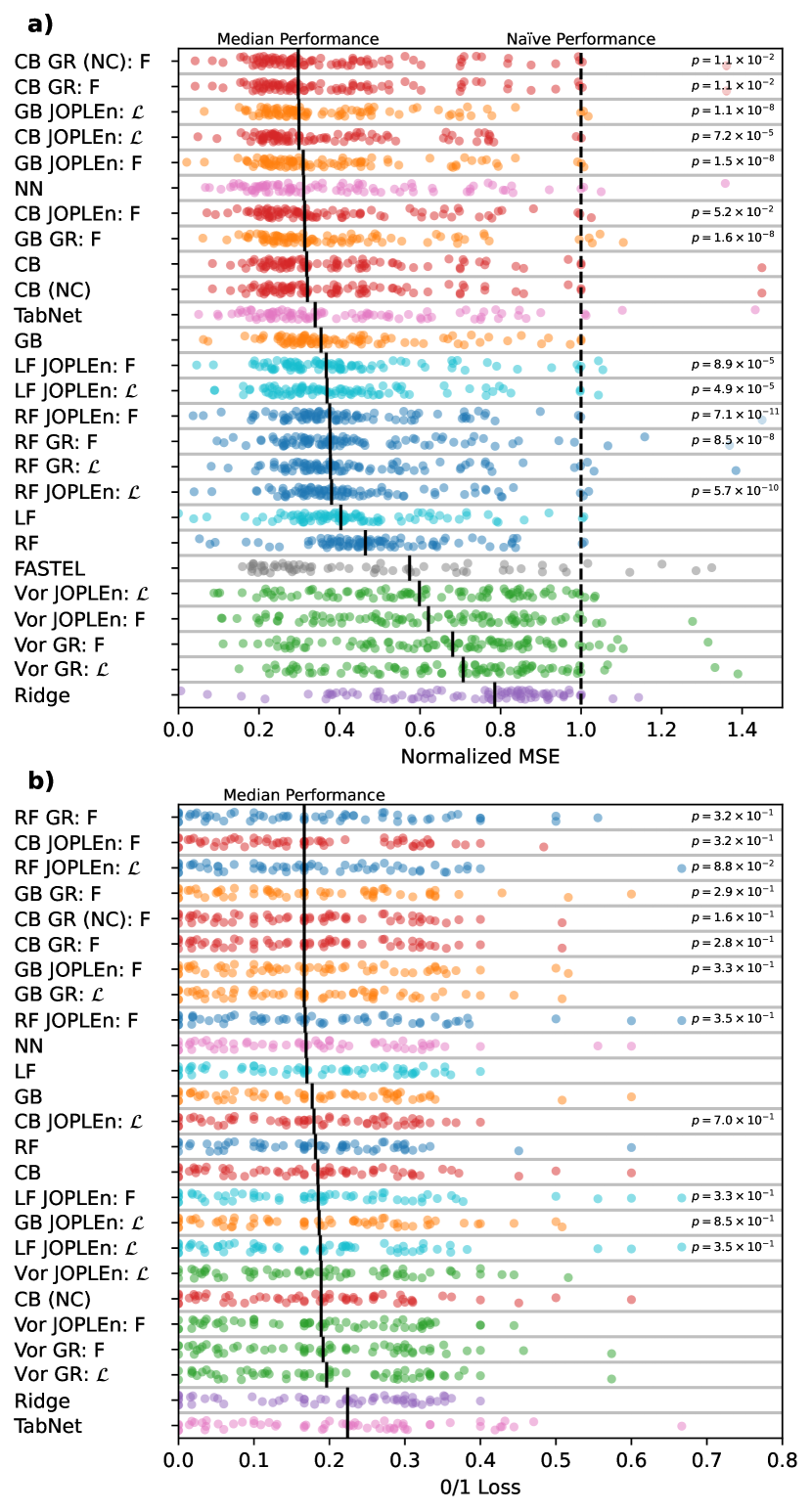
Similar to [3], Figure 1 a) shows that JOPLEn and GR significantly improve the regression performance of GB and RF, as determined by a one-sided Wilcoxon signed-rank test. JOPLEn also significantly improves LF and CB. Indeed, JOPLEn CB $\mathcal{L}$ outperforms all regression approaches including CB ($p=7.2\times 10^{-5}$), despite dropping all categorical features. Based on median performance, CB GR (NC), CB GR, and GB JOPLEn $\mathcal{L}$ appear to outperform JOPLEn CB $\mathcal{L}$. However, JOPLEn CB $\mathcal{L}$ outperforms them with $p=5.6\times 10^{-3}$, $p=4.9\times 10^{-3}$, and $p=8.0\times 10^{-2}$ due to their heavier tail performance.

Although JOPLEn also improves performance for binary classification, the difference is less pronounced ($p=8.8\times 10^{-2}$ for JOPLEn RF $\mathcal{L}$). This decreased significance may be caused by the sample size (60 vs. 90 datasets), or the fact that the 0/1 loss only considers the sign of the prediction.

Interestingly, we observe that the partitioning method may significantly affect performance. In the regression setting, CB, GB, LF, RF, and Voronoi model performances rank in this order. However, there is no significant difference in the classification setting. We suspect that there may be other partitioning methods that lead to further performance increases.

Finally, we note that CB JOPLEn $\mathcal{L}$ outperforms the NNs and FASTEL in general, achieving $p$-values of $3.3\times 10^{-4}$ and $1.5\times 10^{-1}$ for TabNet and the feedforward network. The NNs and FASTEL perform well on many datasets, but have a high median loss because some datasets perform quite poorly. This is particularly true for FASTEL.

In Figure 2 we demonstrate the effect of the nuclear norm on synthetic data. We draw 10,000 samples (100 are training data) uniformly on the square interval $[-1,1]^{2}$, and define $y_{n}\doteq f(\boldsymbol{x}_{n})$ where $f(\boldsymbol{x})\doteq\sin(\pi(x_{1}+x_{2}))+\varepsilon$ for an input feature $\boldsymbol{x}$ and $\varepsilon\sim\mathcal{N}(0,0.2)$. Here, we use random Voronoi ensembles and fix the number of partitions and cells to simplify visualization, and manually tune the penalty weights.

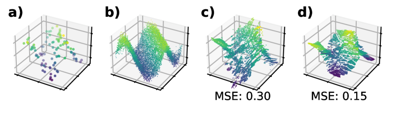
Notably, the nuclear norm causes the model to align its piecewise linear functions along the diagonal, forming a “consensus” across all linear models. By contrast, the Frobenius norm penalty allows each leaf to be optimized independently, and thus suffers from degraded performance.

Next, we show that JOPLEn Dirty LASSO (DL) can achieve superior sparsity to the DL [13].

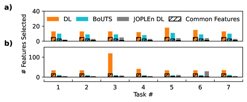
We selected two multitask regression datasets from the literature: NanoChem [7] and SARCOS [25]. NanoChem is a group of 7 small molecule, nanoparticle, and protein datasets for evaluating multitask feature selection performance [7]. These datasets have 1,205 features and 127 to 11,079 samples. The response variables are small molecule boiling point (1), Henry’s constant (2), logP (3) and melting point (4); nanoparticle logP (5) and zeta potential (6); and protein solubility (7). SARCOS is a 7-task dataset that models the dynamics of a robotic arm [25], with 27 features and 48,933 samples for each task. These datasets were also split into train, validation, and test sets using a 0.8/0.1/0.1 ratio.

Using JOPLEn DL with tree ensembles will provide biased sparsity estimates; features are used to create each tree (not penalized) and then to train each linear leaf (penalized). In this case, simply analyzing the leaf weights will underestimate the number of features used by the JOPLEn model. We avoid this issue by using random Voronoi ensembles.

All penalties were manually tuned so that all methods achieve a similar test loss for each task. Not all datasets are equally challenging, so we manually tune the $\gamma^{t}$ parameter for JOPLEn DL and BoUTS. No equivalent parameters exist in the community implementation of DL [26].

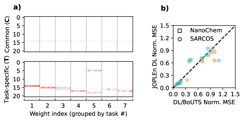
We find that JOPLEn DL and BoUTS select significantly sparser feature sets than DL does, with JOPLEn providing the sparsest sets. Figure 3 a) shows that joint optimization shares penalties across ensemble terms, providing structured sparsity. Further, JOPLEn selects far fewer features than DL (Fig. 4) while achieving similar or superior performance on all but one task (small molecule logP (3), Fig. 3 b)). This is likely because of the significant disparity in the number of features selected for this task (102 for DL, vs. 6 for JOPLEn).

References

- [1] Ravid Shwartz-Ziv and Amitai Armon, “Tabular data: Deep learning is not all you need,” Inform. Fusion, vol. 81, 2022.
- [2] Shibal Ibrahim, Hussein Hazimeh, and Rahul Mazumder, “Flexible modeling and multitask learning using differentiable tree ensembles,” in SIGKDD, 2022.
- [3] Shaoqing Ren, Xudong Cao, Yichen Wei, and Jian Sun, “Global refinement of random forest,” in IEEE CVPR, 2015.
- [4] Hidekazu Oiwa and Ryohei Fujimaki, “Partition-wise linear models,” in NeurIPS, 2014.
- [5] Juan J. Rodríguez, César García-Osorio, Jesús Maudes, and José Francisco Díez-Pastor, “An experimental study on ensembles of functional trees,” in Lect. Notes Comput. Sc., 2010, vol. 5997.
- [6] Zhixiang Xu, Gao Huang, Kilian Q. Weinberger, and Alice X. Zheng, “Gradient boosted feature selection,” in SIGKDD, 2014.
- [7] Matt Raymond, Jacob Charles Saldinger, Paolo Elvati, Clayton Scott, and Angela Violi, “Universal feature selection for simultaneous interpretability of multitask datasets,” arXiv, 2024.
- [8] Guillaume Obozinski, Ben Taskar, and Michael Jordan, “Multi-task feature selection,” Statistics Department, UC Berkeley, Tech. Rep, vol. 2, no. 2.2, 2006.
- [9] Yaohua Hu, Chong Li, Kaiwen Meng, Jing Qin, and Xiaoqi Yang, “Group sparse optimization via regularization,” JMLR, vol. 18, no. 30, 2017.
- [10] Urvashi Oswal, Christopher Cox, Matthew Lambon-Ralph, Timothy Rogers, and Robert Nowak, “Representational similarity learning with application to brain networks,” in ICML, 2016.
- [11] Jeffrey A. Fessler and Raj Rao Nadakuditi, Linear Algebra for Data Science, Machine Learning, and Signal Processing, Cambridge University Press, 2024.
- [12] Neal Parikh and Stephen Boyd, “Proximal algorithms,” Found. Trends Optim., vol. 1, no. 3, Jan 2014.
- [13] Ali Jalali, Sujay Sanghavi, Chao Ruan, and Pradeep Ravikumar, “A dirty model for multi-task learning,” in NeurIPS, 2010.
- [14] Xiaojin Zhu, Zoubin Ghahramani, and John Lafferty, “Semi-supervised learning using gaussian fields and harmonic functions,” in ICML, 2003.
- [15] Joseph D Romano, Trang T Le, William La Cava, et al., “PMLB v1.0: an open source dataset collection for benchmarking machine learning methods,” arXiv, 2021.
- [16] Jerome H. Friedman, “Greedy function approximation: A gradient boosting machine,” Ann. Stat., vol. 29, no. 5, 1999.
- [17] Leo Breiman, “Bagging predictors,” Mach. Learn., vol. 24, no. 2, Aug 1996.
- [18] Liudmila Prokhorenkova, Gleb Gusev, Aleksandr Vorobev, Anna Veronika Dorogush, and Andrey Gulin, “CatBoost: unbiased boosting with categorical features,” in NeurIPS, 2018, vol. 31.
- [19] F. Pedregosa, G. Varoquaux, A. Gramfort, V. Michel, B. Thirion, O. Grisel, M. Blondel, P. Prettenhofer, R. Weiss, V. Dubourg, J. Vanderplas, A. Passos, D. Cournapeau, M. Brucher, M. Perrot, and E. Duchesnay, “SciKit-Learn: Machine learning in Python,” JMLR, vol. 12, 2011.
- [20] Marco Cerliani, “linear-tree,” PyPI, 2022, version 0.3.5.
- [21] Jeffrey Dean, Rajat Monga, et al., “TensorFlow: Large-scale machine learning on heterogeneous systems,” 2015, Software available from tensorflow.org.
- [22] Sercan O. Arik and Tomas Pfister, “TabNet: Attentive interpretable tabular learning,” arXiv, 2020.
- [23] Eduardo Carvalho Pinto and Hartorn Fischman, Sébastien, “Pytorch TabNet,” PyPI, 2019, version 4.1.0.
- [24] Eytan Bakshy, Lili Dworkin, Brian Karrer, Konstantin Kashin, Ben Letham, Ashwin Murthy, and Shaun Singh, “AE: A domain-agnostic platform for adaptive experimentation,” in NeurIPS Systems for ML Workshop, 2018.
- [25] Sethu Vijayakumar, Aaron D’Souza, and Stefan Schaal, “Incremental Online Learning in High Dimensions,” Neural Comput., vol. 17, 12 2005.
- [26] Hicham Janati, “MuTaR: Multi-task regression in Python,” 2019, Github hash: b682ba9.