Joint Optimization of Preamble Selection and Access Barring for Random Access in MTC with General Device Activities
Abstract
Most existing random access schemes for machine-type communications (MTC) simply adopt a uniform preamble selection distribution, irrespective of the underlying device activity distributions. Hence, they may yield unsatisfactory access efficiency. In this paper, we model device activities for MTC as multiple Bernoulli random variables following an arbitrary multivariate Bernoulli distribution which can reflect both dependent and independent device activities. Then, we optimize preamble selection and access barring for random access in MTC according to the underlying joint device activity distribution. Specifically, we investigate three cases of the joint device activity distribution, i.e., the cases of perfect, imperfect, and unknown joint device activity distributions, and formulate the average, worst-case average, and sample average throughput maximization problems, respectively. The problems in the three cases are challenging nonconvex problems. In the case of perfect joint device activity distribution, we develop an iterative algorithm and a low-complexity iterative algorithm to obtain stationary points of the original problem and an approximate problem, respectively. In the case of imperfect joint device activity distribution, we develop an iterative algorithm and a low-complexity iterative algorithm to obtain a Karush-Kuhn-Tucker (KKT) point of an equivalent problem and a stationary point of an approximate problem, respectively. Finally, in the case of unknown joint device activity distribution, we develop an iterative algorithm to obtain a stationary point. The proposed solutions are widely applicable and outperform existing solutions for dependent and independent device activities.
Index Terms:
Machine-type communications (MTC), random access procedure, preamble selection, access barring, optimization.I Introduction
The emerging Internet-of-Things (IoT), whose key idea is to connect everything and everyone by the Internet, has received increasing attention in recent years. Machine-type communications (MTC) are expected to support IoT services and applications, such as home automation, smart grids, smart healthcare, and environment monitoring [2, 3]. Long Term Evolution (LTE) cellular networks offer the most natural and appealing solution for MTC due to ubiquitous coverage. Specifically, the Third-Generation Partnership Project (3GPP) has developed radio technologies, such as LTE-M [4] and Narrowband IoT (NB-IoT) [5], to enhance existing LTE networks and to provide new solutions inherited from LTE, respectively, for better serving IoT use cases. In addition, 3GPP proposes to the International Telecommunications Union (ITU) that LTE-M and NB-IoT should be integrated as part of the fifth generation (5G) specifications [6].
In LTE-M and NB-IoT, devices compete in a random access channel (RACH) to access the base station (BS) through the random access procedure [7]. Specifically, each active device randomly selects a preamble from a pool of available preambles according to a preamble selection distribution, and transmits it during the RACH. The BS acknowledges the successful reception of a preamble if such preamble is transmitted by only one device. In[8, 9, 10, 11, 12, 13, 14, 15, 16, 17, 18], the authors consider the random access procedure and study the effect of preamble selection under certain assumptions on the knowledge of device activities. Specifically,[8, 9, 10, 13, 16, 17, 18] assume that the number of active devices is known; [15, 14] assume that the distribution of the number of active devices is known; [11, 12] assume that the statistics of the data queue of each device are known. In[8, 9, 10, 11, 12, 13, 14, 15, 16, 17, 18], preambles are selected according to a uniform distribution, the average throughput [8, 9, 10, 11, 12, 13, 14, 15, 16, 17, 18], average access efficiency [16] and resource consumption [10] are analyzed and the number of allocated preambles is optimized to maximize the average throughput [10, 17] or access efficiency [16]. Notice that optimal solutions are obtained in [10, 16, 17]. In [19, 20, 21], the active devices are assumed to be known. Under this assumption, each active device is allocated a preamble if the number of preambles is greater than or equal to the number of active devices, and the preambles are allocated to a subset of active devices otherwise.
When many active devices attempt to access a BS simultaneously, a preamble is very likely to be selected by more than one device, leading to a significant decrease in the probability of access success. In this scenario, access control is necessary. One widely used access control method is the access barring scheme [22], which has been included in the LTE specification in [7]. In[8, 9, 10, 11, 12, 13, 14, 15, 16], the authors consider access barring, besides random access procedure with preambles selected according to a uniform distribution. Specifically, the access barring factor is optimized to maximize the average throughput [8, 9, 10, 11, 12, 13, 14] or access efficiency [16], or to minimize the number of backlogged devices [15]. Note that optimal solutions are obtained in [15, 8, 13, 10, 14, 16], an approximate solution is obtained in [9], and asymptotically optimal solutions for a large number of devices are obtained in [11, 12].
There exist two main types of MTC traffic, i.e., event-driven (or event-triggered) traffic and periodic traffic [23, 24]. In event-driven MTC (e.g., smart health care and environment sensing such as rockfall detection and fire alarm), one device being triggered may increase the probability that other devices in the vicinity trigger in quick succession, or many devices are simultaneously triggered in response to a particular IoT event. Hence, device activities can be dependent. Besides, in periodic MTC, devices have their own periods, and hence device activities can be considered independent for tractability (if the periodic behaviors of devices are not tracked). Intuitively, effective preamble selection and access barring should adapt to the statistical behaviors of device activities. Specifically, if devices are more likely to activate simultaneously, letting them always select different preambles can avoid more collisions; if devices are less likely to activate simultaneously, letting them always select the same preamble can avoid more collisions. However, most existing random access schemes simply adopt a uniform preamble selection distribution, irrespective of the underlying device activity distributions [8, 9, 10, 11, 12, 13, 14, 15, 16, 17, 18]. They hence may yield far from optimal access efficiency. This motivates us to model device activities as multiple Bernoulli random variables following an arbitrary multivariate Bernoulli distribution, which can reflect both dependent and independent device activities [25, 26, 27, 28], and optimize preamble selection and access barring according to the multivariate Bernoulli distribution [27]. To our knowledge, [27] is the first work that considers a general joint device activity distribution and attempts to optimize the preamble selection distributions and access barring factors of all devices. More specifically, in [27], the authors assume that a perfect joint device activity distribution is known, maximize an approximation of the average throughput, which captures the active probabilities of every single device and every two devices, and develop a heuristic algorithm to tackle the challenging nonconvex problem. The approximation error and the heuristic algorithm may yield a nonnegligible loss in access efficiency. Therefore, it is critical to explore more effective algorithms adaptive to statistics of device activities. Furthermore, notice that most existing works assume that the number of active devices [8, 9, 10, 13, 16, 17], the distribution of the number of active devices [14, 15], the statistics of the data queue of each device [11, 12], the active devices [19, 20, 21], or the device activity distribution [27] is perfectly known. However, in practice, such assumptions are hardly satisfied. Hence, it is critical to consider the optimization of preamble selection and access barring under imperfect information of device activities or even historical samples of device activities.
This paper investigates the joint optimization of preamble selection and access barring for IoT devices in MTC, whose activities are modeled by an arbitrary multivariate Bernoulli distribution, which can reflect both dependent and independent device activities. Specifically, we consider three cases of the joint device activity distribution, i.e., the case of perfect general joint device activity distribution (where the joint device activity distribution has been perfectly estimated), the case of imperfect joint device activity distribution (where the estimation error of the joint device activity distribution lies within a known deterministic bound), and the case of unknown joint device activity distribution (where activity samples generated according to the joint device activity distribution are available). The optimization-based solutions are generally applicable for any dependent and independent device activities. Our main contributions are summarized below.
-
•
In the case of perfect joint device activity distribution, we formulate the average throughput maximization problem, which is nonconvex with a complicated objective function. Based on the block coordinate descend (BCD) method [29], we develop an iterative algorithm, where most block coordinate optimization problems are solved analytically, and a low-complexity iterative algorithm, where all block coordinate optimization problems have closed-form optimal points, to obtain stationary points of the original problem and an approximate problem, respectively. Furthermore, we characterize an optimality property of a globally optimal point of the original problem.
-
•
In the case of imperfect joint device activity distribution, we formulate the worst-case average throughput maximization problem as a robust optimization problem, which is a max-min problem. By duality theory and successive convex approximation (SCA) [30], we develop an iterative algorithm to obtain a Karush-Kuhn-Tucker (KKT) point of an equivalent problem of the max-min problem. Based on the BCD method, we also develop a low-complexity iterative algorithm, where all block coordinate optimization problems are solved analytically, to obtain a stationary point of an approximate problem of the max-min problem.
-
•
In the case of unknown joint device activity distribution, we formulate the sample average throughput maximization problem, which can be viewed as a nonconvex stochastic optimization problem. Based on mini-batch stochastic parallel SCA [31], we develop an efficient parallel iterative algorithm where the approximate convex problems in each iteration are solved analytically, to obtain a stationary point.
-
•
Finally, we show that for dependent and independent device activities, the proposed solutions achieve significant gains over existing schemes in all three cases by numerical results. Besides, the performance of each low-complexity algorithm is close to that of its counterpart designed for solving the original problem.
The key notation used in this paper is listed in Table I.
| Notation | Description | Notation | Description |
|---|---|---|---|
| the number of devices | the probability that device selects preamble | ||
| the number of preambles | average throughput conditional on | ||
| the activity state of device | average throughput | ||
| the probability that the activity states are | approximate average throughput | ||
| the lower bound of | worst-case average throughput | ||
| the upper bound of | approximate worst-case average throughput | ||
| the access barring factor | sample average throughput |
II System Model
We consider the uplink of a single-cell wireless network consisting of one BS and devices. Let denote the set of devices. We consider a discrete-time system with time being slotted and assume that devices activate independently and identically over slots within a certain period. In each slot, a device can be either active or inactive. Thus, the activities of the devices in a slot can be modeled as Bernoulli random variables, following an arbitrary multivariate Bernoulli distribution [28, 25, 26]. Generally, the Bernoulli random variables (representing the activities of the devices) can be dependent or independent. Let denote the activity state of device , where if device is active and otherwise. Let binary vector denote the activity states of the devices, where . The joint device activity distribution (assumed invariant over the considered period) is denoted by , where represents the probability of the activity states of the devices being . Note that whether the device activities are dependent or independent depends on the values or forms of ’s components. According to the nonnegativity and normalization axioms, we have
| (1a) | |||
| (1b) | |||
In this paper, we consider .111 is not an interesting or practical scenario. We do not pose any additional assumption on . Thus, all analytical and optimization results, relying on or its related quantities, are general.
In a slot, each active device tries to access the BS. Congestion may occur when many active devices require to access the BS at the same time. We adopt an access barring scheme for access control [22]. In particular, at the beginning of each slot, all active devices independently attempt to access the BS with probability , where
| (2a) | |||
| (2b) | |||
Here, is referred to as the access barring factor for all devices and will be optimized later.222The average throughput can be improved when devices have different access barring factors. To avoid resource starvation for each device and maintain fairness, we consider identical access barring factors for all devices in the optimizations for simplicity. The proposed solution framework can be extended to handle different access barring factors. That is, the access barring scheme is parameterized by the access barring factor .
We adopt the random access procedure, which consists of four stages, i.e., preamble transmission, random access response, scheduled transmission, and contention resolution [3]. We focus only on the first stage, which mainly determines the success of access [8, 9, 10, 11, 12, 13, 14, 15, 16, 17, 18, 19, 20, 21, 27]. Consider orthogonal preambles, the set of which is denoted by . Specifically, at the first stage, each device that attempts to access the BS independently selects a preamble out of the preambles to transmit. The probability that device selects preamble is denoted by , which satisfies
| (3a) | |||
| (3b) | |||
Let denote the preamble selection distribution of device . Let denote the distributions of the devices. The -th column of is . Note that for all , the random preamble transmission parameterized by reduces to the preamble transmission in the standard random access procedure [7] when , . Furthermore, note that for all , the considered preamble selection is generally random and becomes deterministic when . We allow , to be arbitrary distributions to maximally avoid the collision.
If a preamble is selected by a single device, this device successfully accesses the BS [11]. Then, the average number of devices that successfully access the BS at activity states in a slot is given by [27]
| (4) |
In this paper, we consider the following three cases of joint device activity distribution and introduce the respective performance metrics.
Perfect joint device activity distribution: In this case, we assume that the joint device activity distribution has been estimated by some learning methods, and the estimation error is negligible. That is, the exact value of is known.
We adopt the average throughput [27]
| (5) | ||||
| (6) |
as the performance metric, where is given by (4). The proof for (6) can be found in Appendix A.
Note that for all ,
represents the probability that all devices in are active and can be computed in advance.
Imperfect joint device activity distribution: In this case, we assume that the joint device activity distribution has been estimated by some learning methods with certain estimation errors.
For all ,
let denote the
estimated probability of the device activity states being , and
let
denote the corresponding estimation error.
Note that
satisfy
, and
for some known estimation error bounds , .
Assume that ,
are known to the BS, but neither nor is known to the BS.
Thus, the BS knows that the exact joint
activity distribution satisfies , where
with and , for all . Note that reflects to a certain extent. It can be easily verified that shrinks to as the estimation error bounds , decrease to . We adopt the worst-case average throughput
| (7) |
as the performance metric, where is given by (6).
Note that with the equality holds if and only if , .
Unknown joint device activity distribution:
In this case, we assume no direct information on the joint device
activity distribution, but samples of the device activity states, generated according to , are available.
The samples reflect to a certain extent via the empirical joint probability distribution, an unbiased estimator of . It can be easily verified that the mean squared error decreases with .
Denote .
For all , the -th sample is denoted by .
We adopt the sample average throughput
| (8) |
as the performance metric, where is given by (4). Note that is a random variable with randomness induced by the samples and .
As illustrated in the introduction, overlooking the joint device activity distribution (or related quantities, such as and , ) may yield ineffective preamble selection and access barring designs. This can be further seen from the following example.
Example 1 (Motivation Example)
We consider devices and preambles. The marginal probability of each device being active is ; the activities of device 1 and device 2 can be correlated (dependent),333Note that correlation (correlated) implies dependence (dependent). and their joint distribution , is given by , , and [26], where represents the correlation coefficient;444The range of is to guarantee that , satisfy (1a)-(1b). and the activity of device 3 is independent of the activities of device 1 and device 2. Thus, is given by . Note that corresponds to dependent device activities, and corresponds to independent device activities. We consider four feasible random access schemes parameterized by , . Specifically, , ,
| (11) |
and (uniform distributions), where represents the column vector of all zeros except the -th entry being , and represents all-one column vector; and
| (14) |
Note that , , and do not rely on , whereas depends on the parameter of , i.e., .
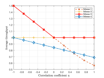
Fig. 1 plots the average throughput versus the correlation efficient . From Fig. 1, we can see that Scheme 3 outperforms Scheme 1 and Scheme 4 at and outperforms Scheme 2 and Scheme 4 at . This is because when device 1 and device 2 are more (or less) likely to activate simultaneously, letting them always select different preambles (or the identical preamble) can avoid more collisions. Besides, Scheme 3 outperforms Scheme 4 at . This example indicates that adapting to can improve the performance of the random access scheme.
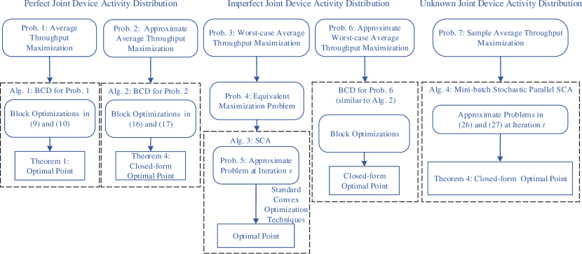
Motivated by Example 1, in Section III, Section IV, and Section V, we shall optimize the preamble selection distributions and access barring factor to maximize the average, worst-case average, and sample average throughputs for given , , and , in the cases of perfect, imperfect, and unknown joint device activity distributions, respectively, as shown in Fig. 2. In what follows, we assume that the optimization problems are solved at the BS given knowledge of , , and , , and the solutions are then sent to all devices for implementation.555In practice, may change slowly over time. For practical implementation, we can re-optimize the preamble selection and access barring using the proposed methods when the change of is sufficiently large, and the obtained stationary point for an outdated generally serves as a good initial point for the latest .
III Performance Optimization for Perfect Joint Device Activity Distribution
In this section, we consider the average throughput maximization in the case of perfect joint device activity distribution. First, we formulate the average throughput maximization problem, which is a challenging nonconvex problem. Then, we develop an iterative algorithm to obtain a stationary point of the original problem. Finally, we develop a low-complexity iterative algorithm to obtain a stationary point of an approximate problem.
A Problem Formulation
In the case of perfect joint device activity distribution, we optimize the preamble selection distributions and access barring factor to maximize the average throughput in (6) subject to the constraints on in (2a), (2b), (3a), and (3b).
Problem 1 (Average Throughput Maximization)
The objective function is nonconcave in , and the constraints in (2a), (2b), (3a), and (3b) are linear, corresponding to a convex feasible set. Thus, Problem 1 is nonconvex with a convex feasible set. In general, a globally optimal point of a nonconvex problem cannot be obtained effectively and efficiently. Obtaining a stationary point is the classic goal for dealing with a nonconvex problem with a convex feasible set.
B Stationary Point
We propose an iterative algorithm based on the BCD method [29], to obtain a stationary point of Problem 1.666One can obtain a stationary point of Problem 1 using SCA [30]. As the approximate convex optimization problem in each iteration has no analytical solution, SCA is not as efficient as the proposed one. Specifically, we divide the variables into blocks, i.e., and . In each iteration of the proposed algorithm, all blocks are sequentially updated. At each step of one iteration, we maximize with respect to one of the blocks. For ease of illustration, in the following, we also write as , where . Given and obtained in the previous step, the block coordinate optimization with respect to is given by
| (15) | |||
Given obtained in the previous step, the block coordinate optimization with respect to is given by
| (16) | |||
Each problem in (15) is a linear program (LP) with variables and constraints. The problem in (16) is a polynomial programming with a single variable and two constraints.
Next, we obtain optimal points of the problems in (15) and (16). Define777Note that , , and .
| (17) |
| (18) |
Denote as the set of roots of equation that lie in the interval . Based on the structural properties of the block coordinate optimization problems in (15) and (16), we can obtain their optimal points.
Proof:
Please refer to Appendix B. ∎
The optimal point in (19) indicates that each device selects the preamble corresponding to the maximum average throughput (increase rate of the average throughput) conditioned on selected by device for given . The overall computational complexity for determining the sets in (19) is , and the overall computational complexity for determining the set in (20) is . The detailed complexity analysis can be found in Appendix C. As is usually sparse during the iterations, the actual computational complexities for obtaining (19) and (20) are much lower.
Finally, the details of the proposed iterative algorithm are summarized in Algorithm 1. Specifically, in Steps , , are updated one by one; in Steps , is updated. Step and Step are to ensure the convergence of Algorithm 1 to a stationary point. Based on the proof for [29, Proposition 2.7.1], we can show the following result.
Theorem 2 (Convergence of Algorithm 1)
Proof:
Please refer to Appendix D. ∎
In practice, we can run Algorithm 1 multiple times (with possibly different random initial points) to obtain multiple stationary points and choose the stationary point with the largest objective value as a suboptimal point of Problem 1.888Generally speaking, finding a good stationary point involves numerical experiments and is more art than technology [32]. However, we find that is generally a good initial point that yields a faster convergence speed with numerical experiments. The intuition is that when , the contending devices for each preamble are statistically balanced irrespective of . The average throughput of the best obtained stationary point and the computational complexity increase with the number of times that Algorithm 1 is run. We can choose a suitable number to balance the increases of the average throughput and computational complexity.
Based on Algorithm 1 and Theorem 2, we can characterize an optimality property of a globally optimal point of Problem 1.
Theorem 3 (Optimality Property)
There exists at least one globally optimal point of Problem 1, which satisfies , for some , .
Proof:
Please refer to Appendix E. ∎
Theorem 3 indicates that there exists a deterministic preamble selection rule that can achieve the maximum average throughput. It is worth noting that the proposed stationary point satisfies the optimality property in Theorem 3. In Section III-C, we shall see that the low-complexity solution also satisfies this optimality property.
C Low-complexity Solution
From the complexity analysis for obtaining a stationary point of Problem 1, we know that Algorithm 1 is computationally expensive when or is large. In this part, we develop a low-complexity algorithm, which is applicable for large or , to obtain a stationary point of an approximate problem of Problem 1. Later, in Section VI, we shall show that the performance of the low-complexity algorithm is comparable with Algorithm 1.
Motivated by the approximations of in [27], we approximate the complicated function , which has terms, with a simpler function
| (21) |
which has terms. The detailed reason for the approximation can be found in [33]. Note that and () represent the probability of device being active and the probability of devices and being active, respectively. By comparing (21) with (6), we can see that captures the active probabilities of every single device and every two devices. Accordingly, we consider the following approximate problem of Problem 1.
Problem 2 (Approximate Average Throughput Maximization)
Analogously, using the BCD method, we propose a computationally efficient iterative algorithm, with more performance guarantee than the heuristic method in [27], to obtain a stationary point of Problem 2. Specifically, variables are divided into blocks, i.e., and . For ease of illustration, we also write as in the sequel. Given and obtained in the previous step, the block coordinate optimization with respect to is given by
| (22) | |||
Given obtained in the previous step, the block coordinate optimization with respect to is given by
| (23) | |||
Each problem in (22) is an LP with variables and constraints, and the problem in (23) is a quadratic program (QP) with a single variable and two constraints. It is clear that the convex problems in (22) and (23) are much simpler than those in (15) and (16), respectively. Based on the structural properties of the block coordinate optimization problems in (22) and (23), we can obtain their optimal points.
The optimal point in (24) indicates that each device selects the preamble with the minimum number of contending devices conditioned on selected by device for given . In the following, we analyze the computational complexity for solving the problems in (22) and (23) according to Theorem 4. As constants and , are computed in advance, the corresponding computational complexities are not considered below. For all and , the computational complexity for calculating is . Furthermore, for all , the computational complexity of finding the largest one among , is . Thus, the overall computational complexity for determining the sets in (24) is . Analogously, the computational complexity for obtaining the closed-form optimal point in (25) is . It is obvious that the computational complexities for obtaining the optimal points given by Theorem 4 are much lower than those for obtaining the optimal points given by Theorem 1. Furthermore, it is worth noting that the optimal points given by Theorem 4 do not rely on the active probabilities of more than two devices.
Finally, the details of the proposed iterative algorithm are summarized in Algorithm 2. Specifically, in Steps , , are updated one by one; in Steps , is updated. Step and Step are to ensure the convergence of Algorithm 2 to a stationary point. Similarly, we have the following results.
Theorem 5 (Convergence of Algorithm 2)
IV Robust Optimization for Imperfect Joint Device Activity Distribution
In this section, we consider the worst-case average throughput maximization in the case of imperfect joint device activity distribution. First, we formulate the worst-case average throughput maximization problem, which is a challenging max-min problem. Then, we develop an iterative algorithm to obtain a KKT point of an equivalent problem. Finally, we develop a low-complexity iterative algorithm to obtain a stationary point of an approximate problem.
A Problem Formulation
In the case of imperfect joint device activity distribution, we optimize the preamble selection distributions and access barring factor to maximize the worst average throughput in (7) subject to the constraints on in (2a), (2b), (3a), and (3b).
Problem 3 (Worst-case Average Throughput Maximization)
Note that we explicitly consider the estimation error of the joint device activity distribution in the optimization. The objective function is nonconcave in , and the constraints in (2a), (2b), (3a), and (3b) are linear. Thus, Problem 3 is nonconvex. Moreover, note that the objective function does not have an analytical form.
B KKT Point
Problem 3 is a challenging max-min problem. In this part, we solve Problem 3 in two steps [34]. First, we transform the max-min problem in Problem 3 to an equivalent maximization problem. As the inner problem is an LP with respect to and strong duality holds for the LP, the inner problem shares the same optimal value as its dual problem. Furthermore, to facilitate algorithm design,999In the constraints in (26c), variables , , and are coupled. Thus, we cannot apply the BCD method to solve Problem 4. we can transform Problem 3 to the following equivalent problem by a change of variables , where .
Problem 4 (Equivalent Problem of Problem 3)
| (26a) | ||||
| (26b) | ||||
| (26c) | ||||
Proof:
Please refer to Appendix F. ∎
Next, based on Lemma 1, we can solve Problem 4 instead of Problem 3. Problem 4 is nonconvex with a nonconvex feasible set, as , in the objective function and the constraint functions in (26c) are nonconcave. Note that obtaining a KKT point is the classic goal for dealing with a nonconvex problem with a nonconvex feasible set. In what follows, we propose an iterative algorithm to obtain a KKT point of Problem 4 using SCA. Specifically, at iteration , we update by solving an approximate convex problem parameterized by obtained at iteration . For notation convenience, define111111Note that , and .
| (27) |
We choose
| (28) |
where denotes the -norm, as an approximate function of the objective function in Problem 4 at iteration . In addition, we choose
| (29) |
as an approximate function of the constraint function for in (26c) at iteration . Note that the concave components of the objective function and the constraint functions in Problem 4 are left unchanged, and the other nonconcave components, i.e., , in the objective function and in (26c) are minorized at , using the concave components based on their second-order Taylor expansions [35]. Then, at iteration , we approximate Problem 4 with the following convex problem.
Problem 5 (Approximate Problem of Problem 4 at Iteration )
First, we analyze the computational complexity for determining the updated objective function and constraint functions of Problem 5. The computational complexity for calculating , is . Given , the computational complexity for calculating is . Note that constants , and are computed in advance. Thus, at iteration , the computational complexity for determining the updated objective function and constraint functions of Problem 5 is . Then, we solve Problem 5. Problem 5 has variables and constraints. Thus, solving Problem 5 by using an interior-point method has computational complexity [32, pp. 8]. After solving Problem 5, we update
| (30a) | |||
| (30b) | |||
where is a positive constant.
Finally, the details of the proposed iterative algorithm are summarized in Algorithm 3. Based on [30, Theorem 1], we can show the following result.
Theorem 6 (Convergence of Algorithm 3)
Proof:
Please refer to Appendix G. ∎
Analogously, we can run Algorithm 3 multiple times (with possibly different random initial points) to obtain multiple stationary points of Problem 4 and choose the KKT point with the largest worst-case average throughput as a suboptimal point of Problem 4, which can also be regarded as a suboptimal point of Problem 3 according to Lemma 1.
C Low-complexity Solution
From the complexity analysis for solving Problem 5, we know that Algorithm 3 is computationally expensive when or is large. In this part, we develop a low-complexity iterative algorithm, which is applicable for large or , to obtain a stationary point of an approximate problem of Problem 3. Later, in Section VI, we shall show that this low-complexity algorithm can achieve comparable performance. First, we approximate the complicated function , which has terms, with a simpler function, which has terms. Specifically, as in Section III.C, we approximate with . Recall that captures the active probabilities of every single device and every two devices. Analogously, we approximate with
Obviously, . Note that contrary to , only the upper and lower bounds on the active probabilities of every single device and every two devices remain. Thus, we approximate with whose analytical form is given in the following lemma.
Lemma 2 (Approximate Worst-case Average Throughput)
Proof:
Please refer to Appendix H. ∎
Next, we consider the following approximate problem of Problem 3.
Problem 6 (Approximate Worst-case Average Throughput Maximization)
where is given by (31).
The numbers of variables and constraints of Problem 6 are and , respectively, which are much smaller than those of Problem 4. Note that and () represent a lower bound on the active probability of every single device and an upper bound on the active probability of every two devices, respectively, and can be computed in advance. Obviously, Problem 6 shares the same form as Problem 2. Thus, we can use a low-complexity iterative algorithm, similar to Algorithm 2, to obtain a stationary point of Problem 6. The details are omitted due to the page limitation.
V Stochastic Optimization for Unknown Joint Device Activity Distribution
In this section, we consider the sample average throughput maximization in the case of unknown joint device activity distribution. We first formulate the sample average throughput maximization problem, which is a challenging nonconvex problem. Then, we develop an iterative algorithm to obtain a stationary point.
A Problem Formulation
In the case of unknown joint device activity distribution, we optimize the preamble selection distributions and access barring factor to maximize the sample average throughput in (8) subject to the constraints on in (2a), (2b), (3a), and (3b).
Problem 7 (Sample Average Throughput Maximization)
The objective function is nonconcave in , and the constraints in (2a), (2b), (3a), and (3b) are linear. Thus, Problem 7 is nonconvex with a convex feasible set. Note that the objective function has terms, and the number of samples is usually quite large in practice. Therefore, directly tackling Problem 7 is not computationally efficient. To reduce the computation time, we solve its equivalent stochastic version (which is given in Appendix I) using a stochastic iterative algorithm.
B Stationary Point
Based on mini-batch stochastic parallel SCA [31], we propose a stochastic algorithm to obtain a stationary point of Problem 7. The main idea is to solve a set of parallelly refined convex problems, each of which is obtained by approximating with a convex function based on its structure and samples in a uniformly randomly selected mini-batch. We partition into disjoint subsets, , each of size (assuming is divisible by ), where . We divide the variables into blocks, i.e., and . This algorithm updates all blocks in each iteration separately in a parallel manner by maximizing approximate functions of .
Specifically, at iteration , a mini-batch denoted by is selected, where follows the uniform distribution over . Let and represent the preamble selection distribution of device and the access barring factor obtained at iteration . Denote . For ease of illustration, in the following, we also write as , where . We choose
as an approximate function of for updating at iteration . Here, is a positive diminishing stepsize satisfying
and is given by
where , , represents the -th element of , and is given by (27). We choose
as an approximate function of for updating at iteration . Here, is a positive constant and is given by
where .
We first solve the following problems for blocks, in a parallel manner. Given and , the optimization problem with respect to is given by
| (32) | ||||
and the optimization problem with respect to is given by
| (33) | ||||
Each problem in (32) is an LP with variables and constraints. The problem in (33) is a QP with a single variable and two constraints. Based on the structural properties of the optimization problems in (32) and (33), we can obtain their optimal points.
Theorem 7 (Optimal Points of Problems in (32) and (33))
A set of optimal points of each optimization problem in (32) is given by
| (34) |
and the optimal point of the optimization problem in (33) is given by
| (35) |
The optimal point in (34) indicates that each device selects the preamble corresponding to the maximum approximate average throughput (increase rate of the average throughput) conditioned on selected by device for given . For all and , the computational complexity for calculating is . For all , the computational complexity of finding the largest one among , is . Thus, the overall computational complexity for determining the sets in (34) is . The computational complexity for calculating is , which is also the computational complexity for obtaining the optimal point in (35).
Then, we update the preamble selection distributions and access barring factor by
| (36a) | |||
| (36b) | |||
where is a positive diminishing stepsize satisfying
Finally, the details of the proposed stochastic parallel iterative algorithm are summarized in Algorithm 4. Based on [36], we can show the following result.
Theorem 8 (Convergence of Algorithm 4)
Proof:
Please refer to Appendix I. ∎
VI Numerical Results
In this section, we evaluate the performance of the proposed solutions121212Algorithm 2 and Algorithm 4 are computationally efficient and can be easily implemented in practical systems with large . Algorithm 1 and Algorithm 3 are computationally expensive but can provide essential benchmarks for designing effective and low-complexity methods. for dependent and independent device activities via numerical results. In the simulation, we adopt the group device activity model in [26]. Specifically, devices are divided into groups, each of size (assuming is divisible by ), the activity states of devices in different groups are independent, and the activity states of devices in one group are the same. Note that when , the device activities are independent; when , the device activities are dependent. Denote . Let denote the set of devices in group . Let denote the activity state of group , where if group is active, and otherwise. Let denote the activity states of all groups. The probability that a group is active is . Then, in the case of perfect joint device activity distribution, the joint device activity distribution is given by
| (39) |
In the case of imperfect joint device activity distribution, the estimated joint device activity distribution is given by
| (42) |
for , we set , , and for , we set
| (45) |
for some . In the case of unknown joint device activity distribution, we consider samples generated according to the joint device activity distribution given by (39). Note that in the three cases, we consider the same underlying joint device activity distribution for a fair comparison. For ease of presentation, in the following, , , and ’s numerical mean in the cases of perfect, imperfect, and unknown joint device activity distributions, i.e., case-pp, case-ip, and case-up, respectively, are referred to as throughput, unless otherwise specified. We evaluate ’s numerical mean by averaging over realizations of , each obtained based on a set of samples. In case-, the proposed stationary point or KKT point is called Prop-, where pp, ip, up. Furthermore, in case-, the proposed low-complexity solution is called Prop-LowComp-, where pp and ip.
We consider three baseline schemes, namely BL-MMPC, BL-MSPC and BL-LTE. In BL-MMPC and BL-MSPC, are obtained by the MMPC and MSPC allocation algorithms and the proposed access barring scheme in [27], respectively. In BL-LTE, we set according to the standard random access procedure of LTE networks [7] and set according to the optimal access control [15], where denotes the average number of active devices. Note that BL-MMPC and BL-MSPC make use of the dependence of the activities of every two devices; BL-LTE does not utilize any information on the dependence of device activities. In case-, the three baseline schemes are referred to as BL-MMPC-, BL-MSPC-, and BL-LTE-, where pp, ip, up. In case-pp, in BL-MMPC-pp and BL-MSPC-pp and in BL-LTE-pp rely on , . In case-ip, in BL-MMPC-ip and BL-MSPC-ip and in BL-LTE-ip rely on , without considering potential estimation errors. In case-up, in BL-MMPC-up and BL-MSPC-up and in BL-LTE-up rely on the empirical joint device activity distribution obtained from the samples. Considering the tradeoff between the throughput and computational complexity, we run each proposed algorithm five times to obtain each point for all considered parameters.
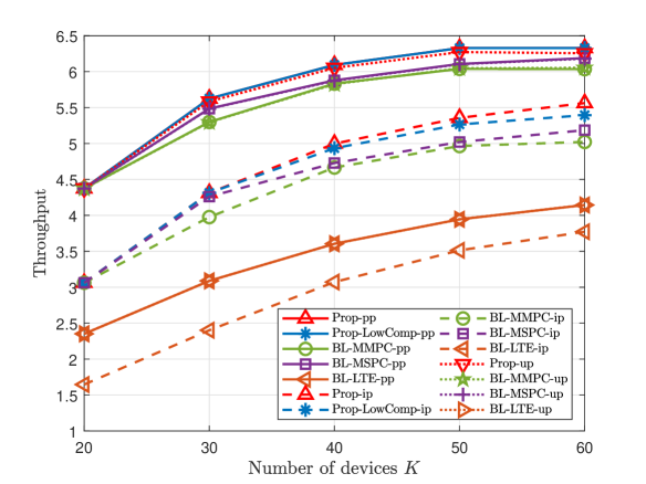
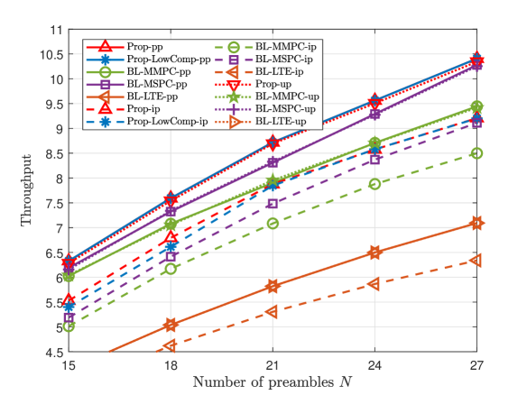
A Small K and N
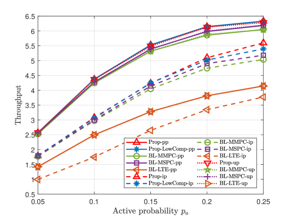
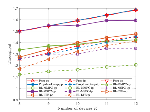
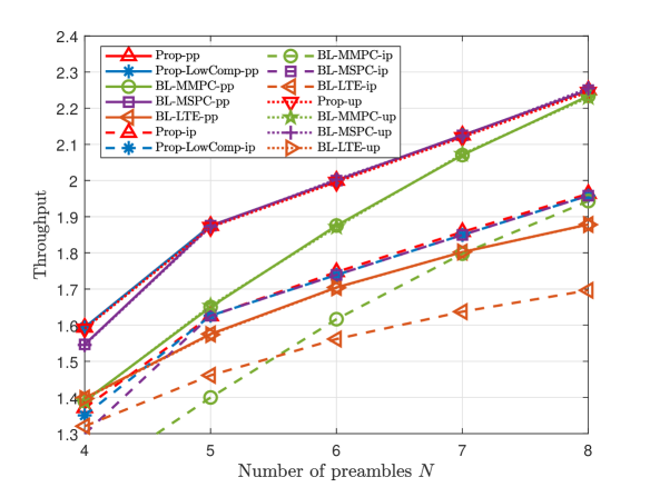
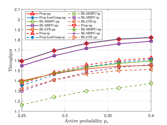
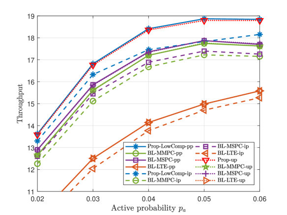
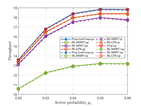
This part compares the throughputs of all proposed solutions and three baseline schemes at small numbers of devices and preambles. Fig. 3 and Fig. 4 illustrate the throughput versus the number of devices , the number of preambles , and the group active probability , for dependent and independent device activities, respectively. From Fig. 3 and Fig. 4, we make the following observations. For each scheme, the curve in case-up is close to that in case-pp, as we evaluate ’s numerical mean over a large number of samples; the curve in case-pp is above that in case-ip, as illustrated in Section II. For pp, ip, and up, Prop- outperforms all the baseline schemes in case-, as Prop- utilizes more statistical information on device activities. For pp and ip, Prop-LowComp- outperforms all the baseline schemes in case-, as Prop-LowComp- relies on a more accurate approximation of the throughput. The fact that the gap between the throughputs of Prop- and Prop-LowComp- is small, where pp and ip, shows that exploiting statistical information on the activities of every two devices rigorously already achieves a significant gain. Furthermore, from Fig. 3 (a), Fig. 4 (a) and Fig. 3 (c), Fig. 4 (c), we can see that the throughput of each proposed scheme increases with and , respectively, due to the increase of traffic load. From Fig. 3 (b) and Fig. 4 (b), we can see that the throughput of each scheme increases with due to the increase of communications resource.
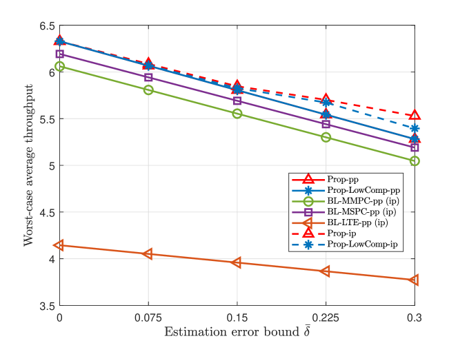
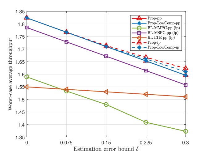
Fig. 6 and Fig. 6 illustrate the worst-case average throughput versus the estimation error bound for dependent and independent device activities, respectively. From Fig. 6 and Fig. 6, we can see the worst-case average throughputs of Prop-ip and Prop-LowComp-ip are greater than those of Prop-pp, Prop-LowComp-pp, BL-MMPC-pp, BL-MSPC-pp, and BL-LTE-pp, which reveals the importance of explicitly considering the imperfectness of the estimated joint device activity distribution in this case. Furthermore, the gain of Prop-ip over Prop-pp and the gain of Prop-LowComp-ip over Prop-LowComp-pp increase with , as it is more important to take into account possible device activity estimation errors when is larger.
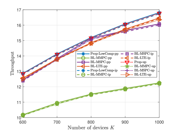
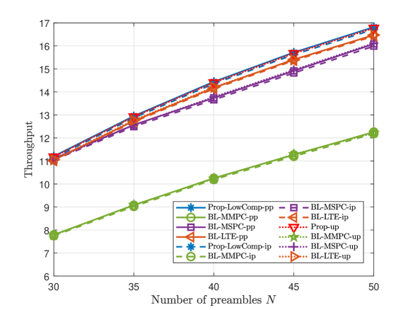
B Large K and N
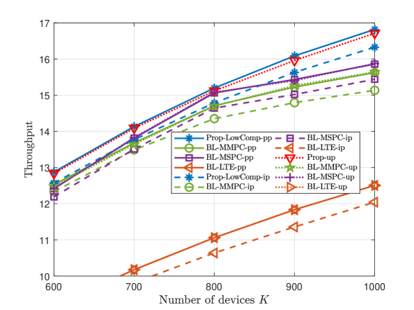
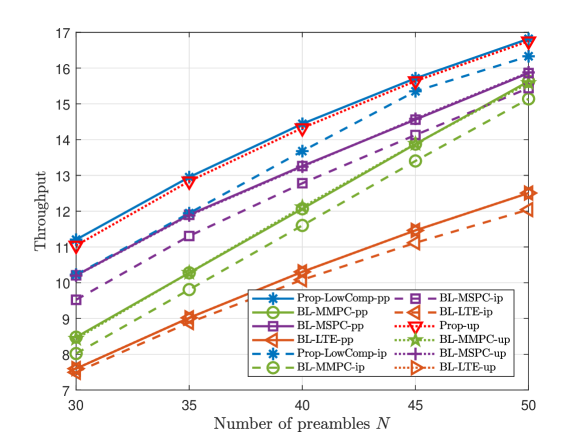
This part compares the throughputs of Prop-LowComp-pp, Prop-LowComp-ip, Prop-up, and three baseline schemes, at large numbers of devices and preambles. Fig. 7 and Fig. 8 illustrate the throughput versus the number of devices , the number of preambles , and the group active probability , for dependent and independent device activities, respectively. From Fig. 7 and Fig. 8, we also observe that Prop-LowComp- significantly outperforms all the baseline schemes in case- for pp and ip; Prop-up outperforms all the baseline schemes in case-up. The results for large and shown in Fig. 7 and Fig. 8 are similar to those for small and shown in Fig. 3 and Fig. 4.
VII Conclusion
This paper considered the joint optimization of preamble selection and access barring for random access in MTC under an arbitrary joint device activity distribution that can reflect dependent and independent device activities. We considered the cases of perfect, imperfect, and unknown general joint device activity distributions and formulated the average, worst-case average, and sample average throughput maximization problems, respectively. All three problems are challenging nonconvex problems. We proposed iterative algorithms with convergence guarantees to tackle these problems with various optimization techniques. Numerical results showed that the proposed solutions achieve significant gains over existing schemes in all three cases for both dependent and independent device activities, and the proposed low-complexity algorithms for the first two cases already achieve competitive performance.
Appendix A: Proof for (6)
Appendix B: Proof of Theorem 1
First, it is clear that each problem in (15) has the same form as the problem in [32, Exercise 4.8]. According to the analytical solution of the problem in [32, Exercise 4.8], a set of optimal points of each problem in (15) are given by (19). Next, since is a polynomial with respect to , by checking all roots of and the endpoints of the interval, we can obtain the set of optimal points of the problem in (16), which is given by (20). Therefore, we complete the proof of Theorem 1.
Appendix C: Complexity analysis for applying Theorem 1
As constants , , and , are computed in advance, the corresponding computational complexities are not considered below. First, we analyze the computational complexity for determining the set in (19). In each iteration, we first compute , in flops. Then, we compute , , . In (17), the summation with respect to contains summands, the summation with respect to contains summands, and for with involves multiplications. Thus, calculating , , costs flops, i.e., has computational complexity . For all , the computational complexity for finding the largest one among is . Thus, the overall computational complexity for determining the sets in (19) is .
Then, we analyze the computational complexity for determining the set in (20). Note that in (18) is a univariate polynomial of order with respect to for any given and . We first calculate the coefficients of . In (18), the summation with respect to contains summands, the summation with respect to and contains summands, and for and with involves multiplications. Thus, calculating the coefficients of costs flops, i.e., has computational complexity . Next, we obtain the roots of based on its coefficients by using the QR algorithm with computational complexity . Furthermore, finding the real roots in from these roots has computational complexity . Hence, the computational complexity for determining is . Analogously, we know that the computational complexity for computing , is . The computational complexity for finding the largest ones among , is . Therefore, the overall computational complexity for determining the set in (20) is .
Appendix D: Proof of Theorem 2
First, we show that Algorithm 1 stops in a finite number of iterations. Let denote the preamble selection distributions and the access barring factor obtained at iteration . contains elements, contains no more than elements. Thus, and both contain no more than elements. In addition, as is nondecreasing with (due to the block coordinate optimizations in each iteration) and , , by contradiction, we can show that there exists an integer such that . According to Steps - in Algorithm 1, we have , which satisfies the stopping criteria of Algorithm 1. Thus, Algorithm 1 stops at iteration , which is no more than iterations. Next, we show that Algorithm 1 returns a stationary point of Problem 1. By and Theorem 1, is the optimal point of the problem in (15) with and , for , and is the optimal point of the problem in (16) with . In addition, note that the objective function is continuously differentiable and the feasible set of Problem 1 is convex. Thus, according to the proof for [29, Proposition 2.7.1], we know that satisfies the first-order optimality condition of Problem 1, i.e., it is a stationary point. Therefore, we complete the proof of Theorem 2.
Appendix E: Proof of Theorem 3
Let denote the vector mapping corresponding to one iteration of Algorithm 1. Let denote an optimal point of Problem 1. We construct a feasible point which satisfies the optimality property in Theorem 3. In the following, we show that is also an optimal point of Problem 1. According to Theorem 1, we have . In addition, as is an optimal point, and is a feasible point, we have . By and , we have , which implies that is also optimal. Therefore, we complete the proof of Theorem 3.
Appendix F: Proof of Lemma 1
The inner problem of Problem 3, , is a feasible LP with respect to for all satisfying (2a), (2b), (3a) and (3b). As strong duality holds for LP, the primal problem, , and its dual problem, share the same optimal value. Furthermore, by eliminating the equality constraints in the dual problem, we can equivalently convert the dual problem to the following problem[33]
| (47) | ||||
Thus, the problems in (47) and share the same optimal value, which can be viewed as a function of . Thus, the max-min problem in Problem 3 can be equivalently converted to the maximization problem in Problem 4, by replacing the inner problem, , with the problem in (47), and replacing with new variables in both the objective function and constraint functions. Therefore, we complete the proof of Lemma 1.
Appendix G: Proof of Theorem 6
We show that the assumptions in [30, Theorem 1] are satisfied. It is clear that and , are continuously differentiable with respect to , and each of them is the sum of linear functions and strongly concave functions. Thus, and , satisfy the first, second, and third assumptions. From (28) and (29), it is clear that and , satisfy the fourth and fifth assumptions. Let and denote the Hessians of and , respectively. We can show , , and [33], where represents the identity matrix. Thus, using the inequality implied by Taylor’s theorem [35, Eq. (25)], we know that and , satisfy the sixth assumption. Therefore, Theorem 4 readily follows from [30, Theorem 1].
Appendix H: Proof of Lemma 2
For all satisfying (2a), (2b), (3a), (3b), as , we have , where the equality holds when
| (49) |
are satisfied. Thus, to show Lemma 2, it is equivalent to show that the system of linear equations with variable in (49) has a solution. Let [37]. Obviously, is a bijection. Thus, for all , we can also write as . As , , , and , are all different, the matrix of the system of linear equations in (49) has full row rank. In addition, note that the number of equations, , is no greater than the number of variables, . Thus, the system of linear equations in (49) has a solution. We complete the proof of Lemma 2.
Appendix I: Proof of Theorem 8
For all and all , let , which is a singleton, and let denote one index in . First, we show that for any , the optimization problem in (32) and the following QP (which is strongly convex),
| (50) | ||||
share the same optimal point. According to Theorem 7, the optimal point of the problem in (32) is . In addition, for any satisfying the constraints in (3a) and (3b), we can show [33]. By noting that the QP in (50) is strongly convex (as ), is also the unique optimal point of the strongly convex QP. Thus, if is a singleton for all and all , Algorithm 4 can be viewed as stochastic parallel SCA in [36], for solving the following stochastic problem
| (51) | ||||
where (index of mini-batch) follows the uniform distribution over , and the expectation is taken over . By noting that , the stochastic problem in (51) is equivalent to Problem 7. Next, we show the convergence of Algorithm 4 by showing that the assumptions in [36, Theorem 1] are satisfied. Obviously, the constraint set of Problem 7 is compact and convex. It is clear that for any , is smooth on the constraint set of Problem 7, and hence it is continuously differentiable and its derivative is Lipschitz continuous. Random variables are bounded and identically distributed. Therefore, Theorem 8 readily follows from[36, Theorem 1].
References
- [1] W. Liu, Y. Cui, L. Ding, J. Sun, Y. Liu, Y. Li, and L. Zhang, “Joint optimization of preamble selection and access barring for MTC with correlated device activities,” in Proc. IEEE ICC Wkshps., Jun. 2021, pp. 1–6.
- [2] Z. Dawy, W. Saad, A. Ghosh, J. G. Andrews, and E. Yaacoub, “Toward massive machine type cellular communications,” IEEE Wireless Commun., vol. 24, no. 1, pp. 120–128, Feb. 2017.
- [3] M. Hasan, E. Hossain, and D. Niyato, “Random access for machine-to-machine communication in LTE-advanced networks: Issues and approaches,” IEEE Commun. Mag., vol. 51, no. 6, pp. 86–93, Jun. 2013.
- [4] R. Ratasuk, N. Mangalvedhe, D. Bhatoolaul, and A. Ghosh, “LTE-M evolution towards 5G massive MTC,” in Proc. IEEE GC Wkshps., Dec. 2017, pp. 1–6.
- [5] Y. Wang, X. Lin, A. Adhikary, A. Grovlen, Y. Sui, Y. Blankenship, J. Bergman, and H. S. Razaghi, “A primer on 3GPP narrowband Internet of Things,” IEEE Commun. Mag., vol. 55, no. 3, pp. 117–123, Mar. 2017.
- [6] E. Dahlman, P. Stefan, and S. Johan, 5G NR: The Next Generation Wireless Access Technology. Academic Press, 2020.
- [7] 3GPP, “Evolved universal terrestrial radio access (E-UTRA); medium access control (MAC) protocol specification,” TS 36.321, Apr, 2015.
- [8] S. Duan, V. Shah-Mansouri, Z. Wang, and V. W. S. Wong, “D-ACB: Adaptive congestion control algorithm for bursty M2M traffic in LTE networks,” IEEE Trans. Veh. Technol., vol. 65, no. 12, pp. 9847–9861, Dec. 2016.
- [9] Z. Wang and V. W. S. Wong, “Optimal access class barring for stationary machine type communication devices with timing advance information,” IEEE Trans. Wireless Commun., vol. 14, no. 10, pp. 5374–5387, Oct. 2015.
- [10] M. Vilgelm, S. Rueda Liares, and W. Kellerer, “On the resource consumption of M2M random access: Efficiency and pareto optimality,” IEEE Wireless Commun. Lett., vol. 8, no. 3, pp. 709–712, Jun. 2019.
- [11] W. Zhan and L. Dai, “Massive random access of machine-to-machine communications in LTE networks: Modeling and throughput optimization,” IEEE Trans. Wireless Commun., vol. 17, no. 4, pp. 2771–2785, Apr. 2018.
- [12] ——, “Massive random access of machine-to-machine communications in LTE networks: Throughput optimization with a finite data transmission rate,” IEEE Trans. Wireless Commun., vol. 18, no. 12, pp. 5749–5763, Apr. 2019.
- [13] C. Di, B. Zhang, Q. Liang, S. Li, and Y. Guo, “Learning automata-based access class barring scheme for massive random access in machine-to-machine communications,” IEEE Internet Things J., vol. 6, no. 4, pp. 6007–6017, Aug. 2019.
- [14] H. Jin, W. T. Toor, B. C. Jung, and J. Seo, “Recursive pseudo-bayesian access class barring for M2M communications in LTE systems,” IEEE Trans. Veh. Technol., vol. 66, no. 9, pp. 8595–8599, Sep. 2017.
- [15] O. Galinina, A. Turlikov, S. Andreev, and Y. Koucheryavy, “Stabilizing multi-channel slotted ALOHA for machine-type communications,” in Proc. IEEE ISIT, Jul. 2013, pp. 2119–2123.
- [16] C. Oh, D. Hwang, and T. Lee, “Joint access control and resource allocation for concurrent and massive access of M2M devices,” IEEE Trans. Wireless Commun., vol. 14, no. 8, pp. 4182–4192, Aug. 2015.
- [17] J. Choi, “On the adaptive determination of the number of preambles in RACH for MTC,” IEEE Wireless Commun. Lett., vol. 20, no. 7, pp. 1385–1388, Jul. 2016.
- [18] ——, “Multichannel ALOHA with exploration phase,” in Proc. IEEE WCNC, May 2020, pp. 1–6.
- [19] M. Shehab, A. K. Hagelskjar, A. E. Kalor, P. Popovski, and H. Alves, “Traffic prediction based fast uplink grant for massive IoT,” in Proc. IEEE PIMRC, Sep. 2020, pp. 1–6.
- [20] S. Ali, A. Ferdowsi, W. Saad, N. Rajatheva, and J. Haapola, “Sleeping multi-armed bandit learning for fast uplink grant allocation in machine type communications,” IEEE Trans. Commun., vol. 68, no. 8, pp. 5072–5086, Apr. 2020.
- [21] S. Ali, W. Saad, and N. Rajatheva, “A directed information learning framework for event-driven M2M traffic prediction,” IEEE Commun. Lett., vol. 22, no. 11, pp. 2378–2381, Aug. 2018.
- [22] 3GPP, “Study on RAN improvements for machine-type communications,” TR 37.868, Spt. 2011.
- [23] E. Soltanmohammadi, K. Ghavami, and M. Naraghi-Pour, “A survey of traffic issues in machine-to-machine communications over LTE,” IEEE Internet Things J., vol. 3, no. 6, pp. 865–884, Dec. 2016.
- [24] J. Navarro-Ortiz, P. Romero-Diaz, S. Sendra, P. Ameigeiras, J. J. Ramos-Munoz, and J. M. Lopez-Soler, “A survey on 5G usage scenarios and traffic models,” IEEE Commun. Surv. Tutor., vol. 22, no. 2, pp. 905–929, May 2020.
- [25] Y. Cui, S. Li, and W. Zhang, “Jointly sparse signal recovery and support recovery via deep learning with applications in MIMO-based grant-free random access,” IEEE J. Select. Areas Commun., vol. 39, no. 3, pp. 788–803, Mar. 2021.
- [26] D. Jiang and Y. Cui, “ML and MAP device activity detections for grant-free massive access in multi-cell networks,” IEEE Trans. Wireless Commun., to appear.
- [27] A. E. Kalor, O. A. Hanna, and P. Popovski, “Random access schemes in wireless systems with correlated user activity,” in Proc. IEEE SPAWC, Jun. 2018, pp. 1–5.
- [28] L. Liu and W. Yu, “Massive connectivity with massive MIMO–part I: Device activity detection and channel estimation,” IEEE Trans. Signal Process., vol. 66, no. 11, pp. 2933–2946, Jun. 2018.
- [29] D. P. Bertsekas, Nonlinear progranmming. Athena scientific Belmont, MA, 1998.
- [30] M. Razaviyayn, “Successive convex approximation: Analysis and applications,” Ph.D. dissertation, Univ. of Minnesota, Minneapolis, MN, USA, May 2014.
- [31] A. Koppel, A. Mokhtari, and A. Ribeiro, “Parallel stochastic successive convex approximation method for large-scale dictionary learning,” in Proc. IEEE ICASSP, Apr. 2018, pp. 2771–2775.
- [32] S. Boyd, S. P. Boyd, and L. Vandenberghe, Convex optimization. Cambridge university press, 2004.
- [33] W. Liu, Y. Cui, F. Yang, L. Ding, and J. Sun, “Joint optimization of preamble selection and access barring for random access in mtc with general device activities,” arXiv preprint arXiv:2107.10461, Jul. 2021.
- [34] C. Ye, Y. Cui, Y. Yang, and R. Wang, “Optimal caching designs for perfect, imperfect, and unknown file popularity distributions in large-scale multi-tier wireless networks,” IEEE Trans. Commun., vol. 67, no. 9, pp. 6612–6625, May 2019.
- [35] Y. Sun, P. Babu, and D. P. Palomar, “Majorization-minimization algorithms in signal processing, communications, and machine learning,” IEEE Trans. Signal Process., vol. 65, no. 3, pp. 794–816, Feb. 2017.
- [36] Y. Yang, G. Scutari, D. P. Palomar, and M. Pesavento, “A parallel decomposition method for nonconvex stochastic multi-agent optimization problems,” IEEE Trans. Signal Process., vol. 64, no. 11, pp. 2949–2964, Feb. 2016.
- [37] J. L. Teugels, “Some representations of the multivariate bernoulli and binomial distributions,” Journal of Multivariate Analysis, vol. 32, no. 2, pp. 256–268, Feb. 1990.