Joint Source-Channel Coding on a Multiple Access Channel with Side Information
Abstract
We consider the problem of transmission of several distributed correlated sources over a multiple access channel (MAC) with side information at the sources and the decoder. Source-channel separation does not hold for this channel. Sufficient conditions are provided for transmission of sources with a given distortion. The source and/or the channel could have continuous alphabets (thus Gaussian sources and Gaussian MACs are special cases). Various previous results are obtained as special cases. We also provide several good joint source-channel coding schemes for discrete sources and discrete/continuous alphabet channel.
Keywords: Multiple access channel, side information, lossy joint source-channel coding, jointly Gaussian codewords, correlated sources.
I Introduction and Survey
In this paper we consider the transmission of information from several correlated sources over a multiple access channel with side information. This system does not satisfy source-channel separation ([12]). Thus for optimal transmission one needs to consider joint source-channel coding. We will provide several good joint source-channel coding schemes.
Although this topic has been studied for last several decades, one recent motivation is the problem of estimating a random field via sensor networks. Sensor nodes have limited computational and storage capabilities and very limited energy [3]. These sensor nodes need to transmit their observations to a fusion center which uses this data to estimate the sensed random field. Since transmission is very energy intensive, it is important to minimize it.
The proximity of the sensing nodes to each other induces high correlations between the observations of adjacent sensors. One can exploit these correlations to compress the transmitted data significantly ([3], [4]). Furthermore, some of the nodes can be more powerful and act as cluster heads ([4]). Nodes transmit their data to a nearby cluster head which can further compress information before transmission to the fusion center. Transmission of data from sensor nodes to their cluster-head requires sharing the wireless multiple access channel (MAC). At the fusion center the underlying physical process is estimated. The main trade-off possible is between the rates at which the sensors send their observations and the distortion incurred in the estimation at the fusion center. The availability of side information at the encoders and/or the decoder can reduce the rate of transmission ([19], [42]).
The above considerations open up new interesting problems in multi-user information theory and the quest for finding the optimal performance for various models of sources, channels and side information have made this an active area of research. The optimal solution is not known except in a few simple cases. In this paper a joint source channel coding approach is discussed under various assumptions on side information and distortion criteria. Sufficient conditions for transmission of discrete/continuous alphabet sources with a given distortion over a discrete/continuous alphabet MAC are provided. These results generalize the previous results available on this problem.
In the following we survey the related literature. Ahlswede [1] and Liao [28] obtained the capacity region of a discrete memoryless MAC with independent inputs. Cover, El Gamal and Salehi [12] made further significant progress by providing sufficient conditions for transmitting losslessly correlated observations over a MAC. They proposed a ‘correlation preserving’ scheme for transmitting the sources. This mapping is extended to a more general system with several principle sources and several side information sources subject to cross observations at the encoders in [2]. However single letter characterization of the capacity region is still unknown. Indeed Duek [15] proved that the conditions given in [12] are only sufficient and may not be necessary. In [26] a finite letter upper bound for the problem is obtained. It is also shown in [12] that the source-channel separation does not hold in this case. The authors of [35] obtain a condition for separation to hold in a multiple access channel.
The capacity region for the distributed lossless source coding problem for correlated sources is given in the classic paper by Slepian and Wolf ([38]). Cover ([11]) extended Slepian-Wolf results to an arbitrary number of discrete, ergodic sources using a technique called ‘random binning’. Other related papers on this problem are [2], [6].
Inspired by Slepian-Wolf results, Wyner and Ziv [42] obtained the rate distortion function for source coding with side information at the decoder. It is shown that the knowledge of side information at the encoders in addition to the decoder, permits the transmission at a lower rate. This is in contrast to the lossless case considered by Slepian and Wolf. The rate distortion function when encoder and decoder both have side information was first obtained by Gray (See [8]). Related work on side information coding is [5], [14], [33]. The lossy version of Slepian-Wolf problem is called multi-terminal source coding problem and despite numerous attempts (e.g., [9], [30]) the exact rate region is not known except for a few special cases. First major advancement was in Berger and Tung ([8]) where an inner and an outer bound on the rate distortion region was obtained. Lossy coding of continuous sources at the high resolution limit is studied in [43] where an explicit single-letter bound is obtained. Gastpar ([19]) derived an inner and an outer bound with decoder side information and proved the tightness of his bounds when the sources are conditionally independent given the side information. The authors in [39] obtain inner and outer bounds on the rate region with side information at the encoders and the decoder. In [29] an achievable rate region for a MAC with correlated sources and feedback is given.
The distributed Gaussian source coding problem is discussed in [30], [41]. For two users exact rate region is provided in [41]. The capacity of a Gaussian MAC (GMAC) for independent sources with feedback is given in [32]. In [27] one necessary and two sufficient conditions for transmitting a bivariate jointly Gaussian source over a GMAC are provided. It is shown that the amplify and forward scheme is optimal below a certain SNR. The performance comparison of the schemes given in [27] with a separation-based scheme is given in [34]. GMAC under received power constraints is studied in [18] and it is shown that the source-channel separation holds in this case.
In [20] the authors discuss a joint source channel coding scheme over a MAC and show the scaling behavior for the Gaussian channel. A Gaussian sensor network in distributed and collaborative setting is studied in [24]. The authors show that it is better to compress the local estimates than to compress the raw data. The scaling laws for a many-to-one data-gathering channel are discussed in [17]. It is shown that the transport capacity of the network scales as when the number of sensors grows to infinity and the total average power remains fixed. The scaling laws for the problem without side information are also discussed in [21] and it is shown that separating source coding from channel coding may require exponential growth, as a function of number of sensors, in communication bandwidth. A lower bound on best achievable distortion as a function of the number of sensors, total transmit power, the degrees of freedom of the underlying process and the spatio-temporal communication bandwidth is given.
The joint source-channel coding problem also bears relationship to the CEO problem [10]. In this problem, multiple encoders observe different, noisy versions of a single information source and communicate it to a single decoder called the CEO which is required to reconstruct the source within a certain distortion. The Gaussian version of the CEO problem is studied in [31].
This paper makes the following contributions. It obtains sufficient conditions for transmission of correlated sources with given distortions over a MAC with side information. The source/channel alphabets can be discrete or continuous. The sufficient conditions are strong enough that previous known results are special cases. Next we obtain a bit to Gaussian mapping which provides correlated Gaussian channel codewords for discrete distributed sources.
The paper is organized as follows. Sufficient conditions for transmission of distributed sources over a MAC with side information and given distortion are obtained in Section II. The sources and the channel alphabets can be continuous or discrete. Several previous results are recovered as special cases in Section III. Section IV considers the important case of transmission of discrete correlated sources over a GMAC and presents a new joint source-channel coding scheme. Section V briefly considers Gaussian sources over a GMAC. Section VI concludes the paper. The proof of the main theorem is given in Appendix A. The proofs of several other results are provided in later appendices.
II Transmission of correlated sources over a MAC
We consider the transmission of memoryless dependent sources, through a memoryless multiple access channel (Fig. 1). The sources and/or the channel input/output alphabets can be discrete or continuous. Furthermore, side information about the transmitted information may be available at the encoders and the decoder. Thus our system is very general and covers many systems studied earlier.
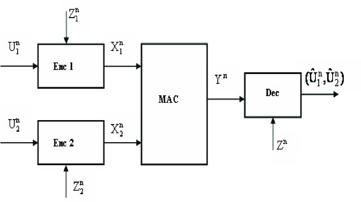
Initially we consider two sources and side information random variables with a known joint distribution . Side information is available to encoder and the decoder has side information . The random vector sequence formed from the source outputs and the side information with distribution is independent identically distributed (iid) in time. We will denote by . Similarly for other sequences. The sources transmit their codewords ’s to a single decoder through a memoryless multiple access channel. The channel output has distribution if and are transmitted at that time. Thus, and satisfy . The decoder receives and also has access to the side information . The encoders at the two users do not communicate with each other except via the side information. The decoder uses the channel outputs and its side information to estimate the sensor observations as . It is of interest to find encoders and a decoder such that can be transmitted over the given MAC with and where are non-negative distortion measures and are the given distortion constraints. If the distortion measures are unbounded we assume that there exist such that . This covers the important special case of mean square error (MSE) if .
Source channel separation does not hold in this case.
For discrete sources a common distortion measure is Hamming distance,
For continuous alphabet sources the most common distortion measure is . To obtain the results for lossless case from our Theorem 1 below, we assume that , e.g., Hamming distance.
: The source can be transmitted over the multiple access channel with distortions if for any there is an such that for all there exist encoders and a decoder such that where and are the sets in which take values.
We denote the joint distribution of by . Also, will denote that form a Markov chain.
Now we state the main Theorem.
Theorem 1
A source can be transmitted over the multiple access channel with distortions if there exist random variables such that
and
(2) there exists a function such that , where and the constraints
| (1) | |||||
are satisfied where are the sets in which take values.
: See Appendix A.
In the proof of Theorem 1 the encoding scheme involves distributed vector quantization of the sources and the side information followed by a correlation preserving mapping to the channel codewords . The decoding approach involves first decoding and then obtaining the estimates as a function of and the decoder side information .
If the channel alphabets are continuous (e.g., GMAC) then in addition to the conditions in Theorem 1 certain power constraints are also needed. In general, we could impose a more general constraint where is some non-negative cost function. Furthermore, for continuous alphabet r.v.s (sources/channel input/output) we will assume that probability density exists so that one can use differential entropy (more general cases can be handled but for simplicity we will ignore them).
The dependence in is used in two ways in (1): to the quantities on the left and to increase the quantities on the right. The side information and effectively the dependence in the inputs.
If the source-channel separation holds then one can consider the capacity region of the channel. For example, when there is no side information and the sources are independent then we obtain the rate region
| (2) |
This is the well known rate region of a MAC ([13]). To obtain (2) from (1), take independent of . Also, take discrete, and independent of .
In Theorem 1 it is possible to include other distortion constraints. For example, in addition to the bounds on one may want a bound on the joint distortion . Then the only modification needed in the statement of the above theorem is to include this also as a condition in defining .
If we only want to estimate a function at the decoder and not themselves, then again one can use the techniques in proof of Theorem 1 to obtain sufficient conditions. Depending upon , the conditions needed may be weaker than those needed in (1). We will explore this in more detail in a later work.
In our problem setup the side information can be included with source and then we can consider this problem as one with no side information at the encoders. However, the above formulation has the advantage that our conditions (1) are explicit in .
The main problem in using Theorem 1 is in obtaining good source-channel coding schemes providing which satisfy the conditions in the theorem for a given source and a channel. A substantial part of this paper will be devoted to this problem.
II-A Extension to multiple sources
The above results can be generalized to the multiple source case. Let be the set of sources with joint distribution .
Theorem 2
Sources can be communicated in a distributed fashion over the memoryless multiple access channel with distortions if there exist auxiliary random variables satisfying
(2) there exists a function such that and the constraints
| (3) |
are satisfied where , is the complement of set and similarly for other r.v.s (in case of continuous channel alphabets we also need the power constraints .
II-B Example
We provide an example to show the reduction possible in transmission rates by exploiting the correlation between the sources, the side information and the permissible distortions.
Consider with the joint distribution: If we use independent encoders which do not exploit the correlation among the sources then we need and for lossless coding of the sources. If we use Slepian-Wolf coding ([38]), then and suffice.
Next consider a multiple access channel such that where and take values from the alphabet and takes values from the alphabet . This does not satisfy the separation conditions in [35]. The sum capacity of such a channel with independent and is and if we use source-channel separation, the given sources cannot be transmitted losslessly because . Now we use a joint source-channel code to improve the capacity of the channel. Take and . Then the sum rate capacity of the channel is improved to . This is still not enough to transmit the sources over the given MAC. Next we exploit the side information.
Let the side-information random variables be generated as follows. is transmitted from source 2 by using a (low rate) binary symmetric channel (BSC) with cross over probability . Similarly is transmitted from source 1 via a similar BSC. Let , where , is a binary random variable with independent of and and ‘.’ denotes the logical AND operation. This denotes the case when the decoder has access to the encoder side information and also has some extra side information. Then from (1) if we use just the side information the sum rate for the sources needs to be . By symmetry the same holds if we only have . If we use and then we can use the sum rate . If only is used then the sum rate needed is . So far we can still not transmit losslessly if we use the coding . If all the information in is used then we need . Thus with the aid of we can transmit losslessly over the MAC even with independent and .
Next we consider the distortion criterion to be the Hamming distance and the allowable distortion as 4%. Then for compressing the individual sources without side information we need , where . Thus we still cannot transmit with this distortion when are independent. Next assume the side information to be available at the decoder only. Then we need where is an auxiliary random variable generated from . This implies that and and we can transmit with independent and .
III Special Cases
In the following we show that our result contains several previous studies as special cases. The practically important special case of GMAC will be studied in detail in later sections. There we will discuss several specific joint source-channel coding schemes for GMAC and compare their performance.
III-A Lossless multiple access communication with correlated sources
Take ( denotes that r.v. is independent of r.v. ) and and where are discrete sources. Then the constraints of (1) reduce to
| (4) |
where . These are the conditions obtained in [12].
If are independent, then and .
III-B Lossy multiple access communication
III-C Lossless multiple access communication with common information
Consider where are independent of each other. is interpreted as the common information at the two encoders. Then, taking , and we obtain sufficient conditions for lossless transmission as
| (6) |
This provides the capacity region of the MAC with common information available in [37].
Our results generalize this result to lossy transmission also.
III-D Lossy distributed source coding with side information
The multiple access channel is taken as a dummy channel which reproduces its inputs. In this case we obtain that the sources can be coded with rates and to obtain the specified distortions at the decoder if
| (7) |
where are obtained by taking .
III-E Correlated sources with lossless transmission over MAC with receiver side information
III-F Mixed Side Information
The aim is to determine the rate distortion function for transmitting a source with the aid of side information (system in Fig 1(c) of [16]). The encoder is provided with and the decoder has access to both and . This represents the Mixed side information (MSI) system which combines the conditional rate distortion system and the Wyner-Ziv system. This has the system in Fig 1(a) and (b) of [16] as special cases.
The results of Fig 1(c) can be recovered from our Theorem if we take in [16] as and . We also take and to be constants. The acceptable rate region is given by , where is a random variable with the property and for which there exists a decoder function such that the distortion constraints are met.
III-G Compound MAC and Interference channel with side information
In compound MAC sources and are transmitted through a MAC which has two outputs and . Decoder is provided with and . Each decoder is supposed to reconstruct both the sources. We take and . We can consider this system as two MAC’s. Applying (1) twice we have for ,
| (9) |
III-H Correlated sources over orthogonal channels with side information
The sources transmit their codewords ’s to a single decoder through memoryless orthogonal channels having transition probabilities and . Hence in the theorem, and . In this case the constraints in (1) reduce to
| (10) | |||||
The outer bounds in (III-H) are attained if the channel codewords are independent of each other. Also, the distribution of maximizing these bounds are not dependent on the distribution of .
Using Fano’s inequality, for lossless transmission of discrete sources over discrete channels with side information, we can show that outer bounds in (III-H) are in fact necessary and sufficient. The proof of the converse is given in Appendix B.
If we take and and the side information , we can recover the necessary and sufficient conditions in [7].
III-I Gaussian sources over a Gaussian MAC
Let be jointly Gaussian with mean zero, variances and correlation . These sources have to be communicated over a Gaussian MAC with the output at time given by where and are the channel inputs at time and is a Gaussian random variable independent of and , with and . The power constaints are . The distortion measure is the mean square error (MSE). We take . We choose and according to the coding scheme given in [27]. and are scaled versions of and respectively. Then from (1) we find that the rates at which and are encoded satisfy
| (11) |
where is the correlation between and . The distortions achieved are
This recovers the sufficient conditions in [27].
IV Discrete Alphabet Sources over Gaussian MAC
This system is practically very useful. For example, in a sensor network, the observations sensed by the sensor nodes are discretized and then transmitted over a GMAC. The physical proximity of the sensor nodes makes their observations correlated. This correlation can be exploited to compress the transmitted data and increase the channel capacity. We present a novel distributed ‘correlation preserving’ joint source-channel coding scheme yielding jointly Gaussian channel codewords which transmit the data efficiently over a GMAC.
Sufficient conditions for lossless transmission of two discrete correlated sources (generating sequences in time) over a general MAC with no side information are obtained in (4).
In this section, we further specialize these results to a GMAC: where is a Gaussian random variable independent of and . The noise satisfies and . We will also have the transmit power constraints: . Since source-channel separation does not hold for this system, a joint source-channel coding scheme is needed for optimal performance.
The dependence of right hand side (RHS) in (4) on input alphabets prevents us from getting a closed form expression for the admissibility criterion. Therefore we relax the conditions by taking away the dependence on the input alphabets to obtain good joint source-channel codes.
Lemma 1
Under our assumptions, .
: See Appendix C.
Thus from (4),
| (12) | |||||
| (13) | |||||
| (14) |
The relaxation of the upper bounds is only in (12) and (13) and not in (14).
We show that the relaxed upper bounds are maximized if is jointly Gaussian and the correlation between and is high (the highest possible may not give the largest upper bound in (12)-(14)).
Lemma 2
A jointly Gaussian distribution for maximizes , and simultaneously.
: See Appendix C.
The difference between the bounds in (12) is
| (15) |
This difference is small if correlation between is small. In that case and will be large and (12) and (13) can be active constraints. If correlation between is large, and will be small and (14) will be the only active constraint. In this case the difference between the two bounds in (12) and (13) is large but not important. Thus, the outer bounds in (12) and (13) are close to the inner bounds whenever the constraints (12) and (13) are active. Often (14) will be the only active constraint.
Based on Lemma 2, we use jointly Gaussian channel inputs with the transmit power constraints. Thus we take with mean vector and covariance matrix . The outer bounds in (12)-(14) become , and respectively. The first two upper bounds decrease as increases. But the third upper bound increases with and often the third constraint is the limiting constraint. Thus, once are obtained we can check for sufficient conditions (4). If these are not satisfied for the obtained, we will increase the correlation between if possible (see details below). Increasing the correlation in will decrease the difference in (15) and increase the possibility of satisfying (4) when the outer bounds in (12) and (13) are satisfied. If not, we can increase further till we satisfy (4).
The next lemma provides an upper bound on the correlation between possible in terms of the distribution of .
Lemma 3
Let be the correlated sources and where and are jointly Gaussian. Then the correlation between satisfies .
: See Appendix C.
It is stated in [35], without proof, that the correlation between cannot be greater than the correlation of the source . Lemma 3 gives a tighter bound in many cases. Consider with the joint distribution: . The correlation between the sources is 0.7778 but from Lemma 3, the correlation between cannot exceed 0.7055.
IV-A A coding Scheme
In this section we develop a distributed coding scheme for mapping the discrete alphabets into jointly Gaussian correlated code words which satisfy (4) and the Markov condition. The heart of the scheme is to approximate a jointly Gaussian distribution with the sum of product of Gaussian marginals. Although this is stated in the following lemma for two dimensional vectors , the results hold for any finite dimensional vectors (hence can be used for any number of users sharing the MAC).
Lemma 4
Any jointly Gaussian two dimensional density can be uniformly arbitrarily closely approximated by a weighted sum of product of marginal Gaussian densities:
| (16) |
: See Appendix C.
From the above lemma we can form a sequence of functions of type (16) such that as , where is a given jointly Gaussian density. Although are not guaranteed to be probability densities, due to uniform convergence, for large , they will almost be. In the following lemma we will assume that we have made the minor modification to ensure that is a proper density for large enough . This lemma shows that obtaining from such approximations can provide the (relaxed) upper bounds in (12)-(14) (we actually show for the third inequality only but this can be shown for the other inequalities in the same way). Of course, as mentioned earlier, then these can be used to obtain the which satisfy the actual bounds in (4).
Let and be random variables with densities and and as . Let and denote the corresponding channel outputs.
Lemma 5
For the random variables defined above, if is uniformly integrable, as .
: See Appendix C.
A set of sufficient conditions for uniform integrability of is
(1) Number of components in (16) is upper bounded.
(2) Variance of component densities in (16) is upper bounded and lower bounded away from zero.
(3) The means of the component densities in (16) are in a bounded set.
From Lemma 4 a joint Gaussian density with any correlation can be expressed by a linear combination of marginal Gaussian densities. But the coefficients and in (16) may be positive or negative. To realize our coding scheme, we would like to have the ’s and ’s to be non negative. This introduces constraints on the realizable Gaussian densities in our coding scheme. For example, from Lemma 3, the correlation between and cannot exceed . Also there is still the question of getting a good linear combination of marginal densities to obtain the joint density for a given in (16).
This motivates us to consider an optimization procedure for finding , , and in (16) that provides the best approximation to a given joint Gaussian density. We illustrate this with an example. Consider to be binary. Let and . Define (notation in the following has been slightly changed compared to (16))
| (17) | |||
| (18) | |||
| (19) | |||
| (20) |
where denotes Gaussian density with mean and variance . Let be the vector with components , , , . Similarly we denote by and the vectors with components , , , and , , ,, ,. The mixture of Gaussian densities (17)-(20) will be used to obtain the RHS in (16) for an optimal approximation. For a given , the resulting joint density is .
Let be the jointly Gaussian density that we want to approximate. Let it has zero mean and covariance matrix . The best is obtained by solving the minimization problem:
| (21) |
subject to
The above constraints are such that the resulting distribution for will satisfy and .
The above coding scheme will be used to obtain a codebook as follows. If user 1 produces , then independently with probability the encoder 1 obtains codeword from the distribution independently of other codewords. Similarly we obtain the codewords for and for user 2. Once we have found the encoder maps the encoding and decoding are as described in the proof of Theorem 1. The decoding is done by joint typicality of the received with .
This coding scheme can be extended to any discrete alphabet case. We give an example below to illustrate the coding scheme.
IV-B Example
Consider with the joint distribution: and power constraints . Also consider a GMAC with . If the sources are mapped into independent channel code words, then the sum rate condition in (14) with should hold. The LHS evaluates to 1.585 bits whereas the RHS is 1.5 bits. Thus (14) is violated and hence the sufficient conditions in (4) are also violated.
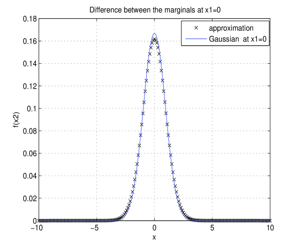
In the following we explore the possibility of using correlated to see if we can transmit this source on the given MAC. The inputs can be distributedly mapped to jointly Gaussian channel code words by the technique mentioned above. The maximum which satisfies upper bounds in (12) and (13) are 0.7024 and 0.7874 respectively and the minimum which satisfies (14) is 0.144. From Lemma 3, is upper bounded by 0.546. Therefore we want to obtain jointly Gaussian satisfying with correlation . If we choose , it meets the inner bounds in (12)-(14) (i.e., the bounds in (4)): , , .
We choose and solve the optimization problem (21) via MATLAB to get the function . The optimal solution solution has both component distributions in (17)- (20) same and these are
The normalized minimum distortion, defined as is 0.137%.
The approximation (a cross section of the two dimensional densities) is shown in Fig. 2.
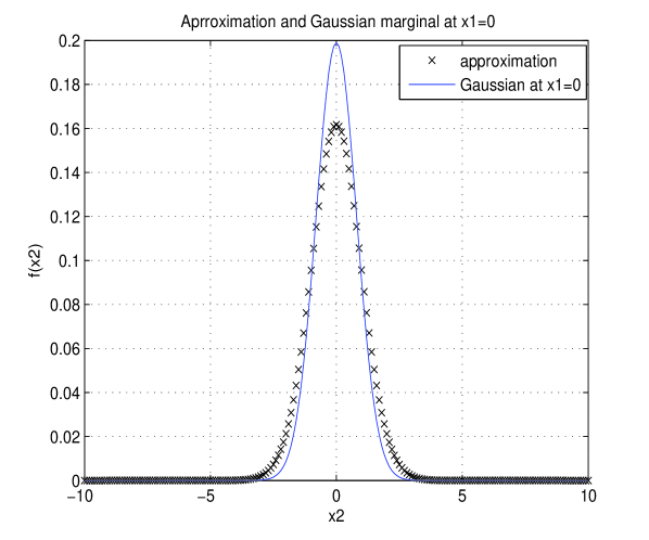
If we take which violates Lemma 3 then the optimal solution from (21) is shown in Fig. 3. We can see that the error in this case is more. Now the normalized marginal distortion is 10.5 %.
IV-C Generalizations
The procedure mentioned in Section IV-A can be extended to systems with general discrete alphabets, multiple sources, lossy transmissions and side information as follows.
Consider users with source taking values in a discrete alphabet . In such a case for each user we find using a mapping mentioned as in (17)-(20) to yield jointly Gaussian .
If and are the side information available, then we use as in (17)-(20) and obtain the optimal approximation from (21).
For lossy transmission, we choose appropriate discrete auxiliary random variables satisfying the conditions in Theorem 1. Then we can form from via the optimization procedure (21).
V Gaussian sources over a GMAC
In this section we consider transmission of correlated Gaussian sources over a GMAC. This is an important example for transmitting continuous alphabet sources over a GMAC. For example one comes across it if a sensor network is sampling a Gaussian random field. Also, in the application of detection of change ([40]) by a sensor network, it is often the detection of change in the mean of the sensor observations with the sensor observation noise being Gaussian.
We will assume that is jointly Gaussian with mean zero, variances and correlation The distortion measure will be Mean Square Error (MSE). The (relaxed) sufficient conditions from (12)-(14) for transmission of the sources over the channel are given by (these continue to hold because Lemmas 1-3 are still valid)
| (22) | |||
where is the correlation between which are chosen to be jointly Gaussian, as in Section IV.
We consider three specific coding schemes to obtain where satisfy the distortion constraints and are jointly Gaussian with an appropriate such that (22) is satisfied. These coding schemes have been widely used. The schemes are Amplify and Forward (AF), Separation Based (SB) and the coding scheme provided in Lapidoth and Tinguely (LT) [27]. We have compared the performance of these schemes in [34]. The AF and LT are joint source-channel coding schemes. In [27] it is shown that AF is optimal at low SNR. In [34] we show that at high SNR LT is close to optimal. SB although performs well at high SNR, is sub-optimal.
For general continuous alphabet sources , no necessarly Gaussian, we vector quantize into . Then to obtain correlated Gaussian codewords we can use the scheme provided in Section IV-A. Alternatively, use Slepian-Wolf coding on . Then for large , and are almost independent. Now on each we can use usual independent Gaussian codebooks as in a point to point channel.
VI Conclusions
In this paper, sufficient conditions are provided for transmission of correlated sources over a multiple access channel. Various previous results on this problem are obtained as special cases. Suitable examples are given to emphasis the superiority of joint source-channel coding schemes. Important special cases of correlated discrete sources over a GMAC and Gaussian sources over a GMAC are discussed in more detail. In particular a new joint source-channel coding scheme is presented for discrete sources over a GMAC.
Appendix A Proof of Theorem 1
The coding scheme involves distributed quantization of the sources and the side information followed by a correlation preserving mapping to the channel codewords. The decoding approach involves first decoding and then obtaining estimate as a function of and the decoder side information .
Let denote the weakly -typical set of sequences of length for where is an arbitrarily small fixed positive constant. We use the following Lemmas in the proof.
Markov Lemma: Suppose . If for a given , is drawn according to , then with high probability for sufficiently large.
The proof of this Lemma for strong typicality is given in [8]. We need it for weak typicality. By the Markov property, formed in the statement of the Lemma has the same joint distribution as the original sequence . Thus the statement of the above Lemma follows. In the same way the following Lemma also holds.
Extended Markov Lemma: Suppose and . If for a given , and are drawn respectively according to and , then with high probability ,, for sufficiently large.
We show the achievability of all points in the rate region (1).
: Fix as well as satisfying the distortion constraints. First we give the proof for the discrete channel alphabet case.
: Let for some . Generate codewords of length , sampled iid from the marginal distribution . For each independently generate sequence according to . Call these sequences . Reveal the codebooks to the encoders and the decoder.
: For , given the source sequence and , the encoder looks for a codeword such that and then transmits .
: Upon receiving , the decoder finds the unique pair such that
. If it fails to find such a unique pair, the decoder declares an error and incurres a maximum distortion of (we assume that the distortion measures are bounded; at the end we will remove this condition).
In the following we show that the probability of error for this encoding-decoding scheme tends to zero as . The error can occur because of the following four events E1-E4. We show that , for .
E1 The encoders do not find the codewords. However from rate distortion theory ([13], page 356), if .
E2 The codewords are not jointly typical with . Probability of this event goes to zero from the extended Markov Lemma.
E3 There exists another codeword such that ,
. Define . Then,
| (23) |
The probability term inside the summation in (23) is
But from hypothesis, we have
Hence,
| (24) |
Then from (23)
In (A) we have used the fact that
The RHS of (A) tends to zero if .
Similarly, by symmetry of the problem we require .
E4 There exist other codewords and such that . Then,
| (26) | |||||
The probability term inside the summation in (26) is
But from hypothesis, we have
Hence,
| (27) |
Then from (26)
The RHS of the above inequality tends to zero if .
Thus as , with probability tending to 1, the decoder finds the correct sequence which is jointly weakly -typical with .
The fact that is weakly -typical with does not guarantee that will satisfy the distortions . For this, one needs that is distortion--weakly typical ([13]) with . Let denote the set of distortion typical sequences. Then by strong law of large numbers as . Thus the distortion constraints are also satisfied by obtained above with a probability tending to 1 as . Therefore, if distortion measure is bounded .
For continuous channel alphabet case (e.g., GMAC) one also needs transmission constraints . For this we need to ensure that the coding scheme chooses a distribution which satisfies . Then if a specific codeword does not satisfy , one declares an error. As this happens with a vanishingly small probability.
If there exist such that , then the result extends to unbounded distortion measures also as follows. Whenever the decoded are not in the distortion typical set then we estimate as . Then for ,
| (28) |
Since and as , the last term of (28) goes to zero as .
Appendix B Proof of converse for lossless transmission of discrete correlated sources over orthogonal channels with side information
Let be the probability of error in estimating from . For any given coding-decoding scheme, we will show that if then the inequalities in (III-H) specialized to the lossless transmission must be satisfied for this system.
Let be the cardinality of set . From Fano’s inequality we have
Denote by . As .
Since,
we obtain . Therefore, because is an iid sequence,
| (29) | |||||
Also, by data processing inequality,
| (30) | |||||
But,
| (31) | |||||
The inequality in the second line is due to the fact that conditioning reduces entropy and the equality in the fifth line is due to the memoryless property of the channel.
We can introduce time sharing random variable as done in [13] and show that . This simplifies to .
By the symmetry of the problem we get .
We also have
But
Also,
Then, following the steps used above, we obtain .
Appendix C Proofs of Lemmas in Section 4
Proof of Lemma 1: Let . Then denoting differential entropy by ,
Since the channel is memoryless, . Thus, .
Proof of Lemma 2: Since
it is maximized when is maximized. This entropy is maximized when is Gaussian with the largest possible variance . If is jointly Gaussian then so is .
Next consider . This equals
which is maximized when is Gaussian and this happens when are jointly Gaussian.
A similar result holds for .
Proof of Lemma 3: Since is a Markov chain, by data processing inequality . Taking to be jointly Gaussian with zero mean, unit variance and correlation . This implies .
Proof of Lemma 4: By Stone-Weierstrass theorem ([25], [36]) the class of functions can be shown to be dense in under uniform convergence where is the set of all continuous functions on such that . Since the jointly Gaussian density is in , it can be approximated arbitrarily closely uniformly by the functions (16).
Proof of Lemma 5: Since
it is sufficient to show that . From and independence of from , we get . Then uniformly implies that . Since and being continuous except at , we obtain . Then uniform integrability provides .
References
- [1] R. Ahlswede. Multiway communication channels. Proc. Second Int. Symp. Inform. Transmission, Armenia, USSR, Hungarian Press, 1971.
- [2] R. Ahlswede and T. Han. On source coding with side information via a multiple access channel and related problems in information theory. IEEE Trans. Inform. Theory, 29(3):396–411, May 1983.
- [3] I. F. Akylidiz, W. Su, Y. Sankarasubramaniam, and E. Cayirici. A survey on sensor networks. IEEE Communications Magazine, pages 1–13, Aug. 2002.
- [4] S. J. Baek, G. Veciana, and X. Su. Minimizing energy consumption in large-scale sensor networks through distributed data compression and hierarchical aggregation. IEEE JSAC, 22(6):1130–1140, Aug. 2004.
- [5] R. J. Barron, B. Chen, and G. W. Wornell. The duality between information embedding and source coding with side information and some applications. IEEE Trans. Inform. Theory, 49(5):1159–1180, May 2003.
- [6] J. Barros and S. D. Servetto. Reachback capacity with non-interfering nodes. Proc.ISIT, pages 356–361, 2003.
- [7] J. Barros and S. D. Servetto. Network information flow with correlated sources. IEEE Trans. Inform. Theory, 52(1):155–170, Jan 2006.
- [8] T. Berger. Multiterminal source coding. Lecture notes presented at 1977 CISM summer school, Udine, Italy, July. 1977.
- [9] T. Berger and R. W. Yeung. Multiterminal source coding with one distortion criterion. IEEE Trans. Inform. Theory, 35(2):228–236, March 1989.
- [10] T. Berger, Z. Zhang, and H. Viswanathan. The CEO problem. IEEE Trans. Inform. Theory, 42(3):887–902, May 1996.
- [11] T. M. Cover. A proof of the data compression theorem of Slepian and Wolf for ergodic sources. IEEE Trans. Inform. Theory, 21(2):226–228, March 1975.
- [12] T. M. Cover, A. E. Gamal, and M. Salehi. Multiple access channels with arbitrarily correlated sources. IEEE Trans. Inform. Theory, 26(6):648–657, Nov. 1980.
- [13] T. M. Cover and J. A. Thomas. Elements of Information theory. Wiley Series in Telecommunication, N.Y., 2004.
- [14] S. C. Draper and G. W. Wornell. Side information aware coding stategies for sensor networks. IEEE Journal on Selected Areas in Comm., 22:1–11, Aug 2004.
- [15] G. Dueck. A note on the multiple access channel with correlated sources. IEEE Trans. Inform. Theory, 27(2):232–235, March 1981.
- [16] M. Fleming and M. Effros. On rate distortion with mixed types of side information. IEEE Trans. Inform. Theory, 52(4):1698–1705, April 2006.
- [17] H. E. Gamal. On scaling laws of dense wireless sensor networks: the data gathering channel. IEEE Trans. Inform. Theory, 51(3):1229–1234, March 2005.
- [18] M. Gastpar. Multiple access channels under received-power constraints. Proc. IEEE Inform. Theory Workshop, pages 452–457, 2004.
- [19] M. Gastpar. Wyner-ziv problem with multiple sources. IEEE Trans. Inform. Theory, 50(11):2762–2768, Nov. 2004.
- [20] M. Gastpar and M. Vetterli. Source-channel communication in sensor networks. Proc. IPSN’03, pages 162–177, 2003.
- [21] M. Gastpar and M. Vetterli. Power spatio-temporal bandwidth and distortion in large sensor networks. IEEE JSAC, 23(4):745–754, 2005.
- [22] D. Gunduz and E. Erkip. Interference channel and compound mac with correlated sources and receiver side information. IEEE ISIT 07, June 2007.
- [23] D. Gunduz and E. Erkip. Transmission of correlated sources over multiuser channels with receiver side information. UCSD ITA Workshop, San Diego, CA, Jan 2007.
- [24] P. Ishwar, R. Puri, K. Ramchandran, and S. S. Pradhan. On rate constrained distributed estimation in unreliable sensor networks. IEEE JSAC, pages 765–775, 2005.
- [25] J. Jacod and P. Protter. Probability Essentials. Springer, N.Y., 2004.
- [26] W. Kang and S. Ulukus. An outer bound for mac with correlated sources. Proc. 40 th annual conference on Information Sciences and Systems, pages 240–244, March 2006.
- [27] A. Lapidoth and S. Tinguely. Sending a bi- variate Gaussian source over a Gaussian MAC. IEEE ISIT 06, 2006.
- [28] H. Liao. Multiple access channels. Ph.D dissertion, Dept. Elec. Engg., Univ of Hawaii, Honolulu, 1972.
- [29] L. Ong and M. Motani. Coding stategies for multiple-access channels with feedback and correlated sources. IEEE Trans. Inform. Theory, 53(10):3476–3497, Oct 2007.
- [30] Y. Oohama. Gaussian multiterminal source coding. IEEE Trans. Inform. Theory, 43(6):1912–1923, Nov. 1997.
- [31] Y. Oohama. The rate distortion function for quadratic Gaussian CEO problem. IEEE Trans. Inform. Theory, 44(3):1057–1070, May 1998.
- [32] L. H. Ozarow. The capacity of the white Gaussian multiple access channel with feedback. IEEE Trans. Inform. Theory, 30(4):623 – 629, July 1984.
- [33] S. S. Pradhan, J. Chou, and K. Ramachandran. Duality between source coding and channel coding and its extension to the side information case. IEEE Trans. Inform. Theory, 49(5):1181–1203, May 2003.
- [34] R. Rajesh and V. Sharma. Source channel coding for Gaussian sources over a Gaussian multiple access channel. Proc. 45 Allerton conference on computing control and communication, Monticello, IL, 2007.
- [35] S. Ray, M. Medard, M. Effros, and R. Kotter. On separation for multiple access channels. Proc. IEEE Inform. Theory Workshop, 2006.
- [36] H. L. Royden. Real analysis. Prentice Hall, Inc., Eaglewood cliffs, New Jersey, 1988.
- [37] D. Slepian and J. K. Wolf. A coding theorem for multiple access channels with correlated sources. Bell syst. Tech. J., 52(7):1037–1076, Sept. 1973.
- [38] D. Slepian and J. K. Wolf. Noiseless coding of correlated information sources. IEEE Trans. Inform. Theory, 19(4):471–480, Jul. 1973.
- [39] V. K. Varsheneya and V. Sharma. Lossy distributed source coding with side information. Proc. National Conference on Communication (NCC), New Delhi, Jan 2006.
- [40] V. V. Veeravalli. Decentralized quickest change detection. IEEE Trans. Inform. Theory, 47(4):1657–1665, May 2001.
- [41] A. B. Wagner, S. Tavildar, and P. Viswanath. The rate region of the quadratic Gaussian two terminal source coding problem. IEEE Trans. Inform. Theory, 54(5):1938–1961, May 2008.
- [42] A. Wyner and J. Ziv. The rate distortion function for source coding with side information at the receiver. IEEE Trans. Inform. Theory, IT-22:1–11, Jan. 1976.
- [43] R. Zamir and T. Berger. Multiterminal source coding with high resolution. IEEE Trans. Inform. Theory, 45(1):106–117, Jan. 1999.